Isovector charges of the nucleon from 2+1-flavor QCD with clover fermions

Abstract

We present high-statistics estimates of the isovector charges of the nucleon from four 2+1-flavor ensembles generated using Wilson-clover fermions with stout smearing and tree-level tadpole improved Symanzik gauge action at lattice spacings $a\approx 0.127$ and $0.09$ fm and with $M_{\pi}\approx 280$ and 170 MeV. The truncated solver method with bias correction and the coherent source sequential propagator construction are used to cost-effectively achieve $O(10^{5})$ measurements on each ensemble. Using these data, the analysis of two-point correlation functions is extended to include four states in the fits, and of three-point functions to three states. Control over excited-state contamination in the calculation of the nucleon mass, the mass gaps between excited states, and in the matrix elements is demonstrated by the consistency of estimates using this multistate analysis of the spectral decomposition of the correlation functions and from simulations of the three-point functions at multiple values of the source-sink separation. The results for all three charges, $g_{A}$, $g_{S}$ and $g_{T}$, are in good agreement with calculations done using the clover-on-HISQ lattice formulation with similar values of the lattice parameters.

I Introduction

This work presents high-statistics estimates of isovector charges of the nucleon, $g_{A}^{u-d}$, $g_{S}^{u-d}$ and $g_{T}^{u-d}$, on four ensembles of (2+1)-flavor lattice QCD using clover-Wilson fermions and a stout smeared tree-level tadpole-improved Symanzik gauge action Edwards et al. (2016). With increased precision, we demonstrate control over excited-state contamination using a multistate analysis of the spectral decomposition of the correlation functions.

Nucleon charges play an important role in the analysis of standard model (SM) and beyond the standard model (BSM) physics. The nucleon axial charge $g_{A}^{u-d}$ is an important parameter that encapsulates the strength of weak interactions of nucleons. The ratio, $g_{A}^{u-d}/g_{V}^{u-d}$, is best determined from the experimental measurement of neutron beta decay using polarized ultracold neutrons by the UCNA Collaboration, $1.2756(30)$ Mendenhall et al. (2013), and by PERKEO II, $1.2761{}^{+14}_{-17}$ Mund et al. (2013). In the SM, $g_{V}^{u-d}=1$ up to second order corrections in isospin breaking Ademollo and Gatto (1964); Donoghue and Wyler (1990) as a result of the conservation of the vector current. Since $g_{A}^{u-d}$ is so well measured, it serves to benchmark lattice QCD calculations and our goal is to provide estimates with $1\%$ total uncertainty.

The isovector charges $g_{S}^{u-d}$ and $g_{T}^{u-d}$, combined with the helicity-flip parameters $b$ and $b_{\nu}$ extracted from the measurements of the neutron decay distribution, probe novel scalar and tensor interactions at the TeV scale Bhattacharya et al. (2012). Assuming that $b$ and $b_{\nu}$ are measured at the $10^{-3}$ precision level Alarcon et al. (2007); Wilburn et al. (2009); Pocanic et al. (2009), one requires that $g_{S}^{u-d}$ and $g_{T}^{u-d}$ be calculated with a precision of 10%–15% Bhattacharya et al. (2012). This precision has recently been reached using the clover-on-HISQ lattice formulation Bhattacharya et al. (2016) and the current clover-on-clover analysis is a necessary independent check using a unitary lattice QCD formulation. The tensor charge is also given by the zeroth moment of the transversity distributions that are measured in many experiments including Drell-Yan and semi-inclusive deep inelastic scattering (SIDIS). Accurate calculations of the contributions of the up and down quarks to the tensor charges will continue to help elucidate the structure of the nucleon in terms of quarks and gluons and provide a benchmark against which phenomenological estimates utilizing a new generation of experiments at Jefferson Lab (JLab) can be compared Dudek et al. (2012). We also use the conserved vector current relation to determine the neutron-proton mass difference in QCD by combining the estimates of $g_{S}^{u-d}/g_{V}^{u-d}$ with the difference of light quarks masses $(m_{d}-m_{u})^{\rm QCD}=2.67(35)$ MeV obtained from independent lattice QCD calculations González-Alonso and Martin Camalich (2014); Bhattacharya et al. (2016).

Most extensions of the Standard Model designed to explain nature at the TeV scale have new sources of $CP$ violation, and the neutron electric dipole moment (EDM) is a very sensitive probe of these. Planned experiments aim to reduce the current bound on the neutron EDM of $2.9\times 10^{-26}\ e$ cm Baker et al. (2006) to around $10^{-28}\ e$ cm. To put stringent constraints on many BSM theories, one requires that matrix elements of novel $CP$-violating interactions, of which the quark EDM is one, are calculated with the required precision. The contributions of the $u,\ d,\ s,\ c$ quark EDM to the neutron EDM Bhattacharya et al. (2015); Pospelov and Ritz (2005) are given by the flavor diagonal tensor charges. Precise results for the connected contributions to these charges from 2+1+1-flavor clover-on-HISQ lattice formulation have been reported in Bhattacharya et al. (2016). Here we present results from a similar high statistics study using the clover-on-clover formulation. The needed contributions of disconnected diagrams are being done in a separate study Gambhir et al. (2016).

The methodology for the lattice QCD calculations of the matrix elements of quark bilinear operators within the nucleon state is well-developed Lin (2012); Syritsyn (2014); Green (2016); Constantinou (2014); Bhattacharya et al. (2015, 2016). Our goal is to first calculate the charges ${g_{\Gamma}}(a,M_{\pi},M_{\pi}L)$ as functions of the lattice spacing $a$, the quark mass characterized by the pion mass $M_{\pi}$ and the lattice size $L$ expressed in dimensionless units of $M_{\pi}L$. After renormalization of these lattice estimates, physical results will be obtained by taking the continuum limit ($a\rightarrow 0$), the physical pion mass limit (set by $M_{\pi^{0}}=135$ MeV) and the infinite volume limit ($M_{\pi}L\rightarrow\infty$) using a combined fit in these three variables Bhattacharya et al. (2016, 2015). Here, we present results for four ensembles at lattice spacings $a\approx 0.127$ and $0.09$ fm with $M_{\pi}\approx 280$ and $170$ MeV. These ensembles are labeled $a127m285$, $a094m280$, $a091m170$, and $a091m170L$ and described in Table 1.

In this work, we demonstrate that precise estimates for matrix elements within nucleon states can be obtained by combining the all-mode-averaging (AMA) error-reduction technique Bali et al. (2010); Blum et al. (2013) (Sec. II.4) and the coherent source sequential propagator method Bratt et al. (2010); Yoon et al. (2016). A detailed analysis of excited-state contamination, comparing the variational method and the 2-state fit to data at multiple source-sink separations $t_{\rm sep}$, was presented in Yoon et al. (2016) using the $a094m280$ ensemble. In this work, we extend the 2-state fit results presented there by doing the calculation at an additional value of the lattice spacing ($a127m285$) and at a lighter pion mass on two ensembles with different volumes ($a091m170$ and $a091m170L$).

The high statistics data allow us to perform a first analysis including up to four states in fits to the two-point correlators and three states in fits to the three-point functions. To obtain results for the charges in the limit that the source-sink separation $\mathop{t_{\rm sep}\to\infty}\nolimits$, we generate data at 4–5 values of $\mathop{t_{\rm sep}}\nolimits$ on each ensemble. Using these data we perform a detailed comparison of results obtained using 2-state versus 3-state fits. Our final estimates of the charges are from 3-state fits.

The renormalization constants of the various quark bilinear operators are calculated on three ensembles $a127m285$, $a094m280$, $a091m170$ in the RI-sMOM scheme and then converted to the $\overline{\text{MS}}$ scheme at $2$ GeV using 2-loop matching and 3-loop running. Our final estimates of the renormalized isovector charges of the nucleon in the $\overline{\text{MS}}$ scheme at $2$ GeV are given in Table 15. Results for the connected part of the flavor diagonal charges are given in Table 16.

Estimates of all three isovector charges, $g_{A}^{u-d}$, $g_{S}^{u-d}$ and $g_{T}^{u-d}$ and of the flavor diagonal charges $g_{A,S,T}^{u,d}$ are in very good agreement with similar high precision calculations done using a 2+1+1-flavor clover-on-HISQ formulation Bhattacharya et al. (2016). Our estimates of $g_{A}$ obtained with heavy $u$ and $d$ quark masses corresponding to $M_{\pi}\approx 280$ and $170$ MeV are within $5\%$ of the experimental result, $1.276(3)$, from neutron beta decay Mendenhall et al. (2013); Mund et al. (2013).

This paper is organized as follows. In Sec. II, we describe the parameters of the gauge ensembles analyzed and the various methods used to obtain high precision results. Two-state fits to two- and three-point functions to extract the unrenormalized charges are presented in Sec. III along with a discussion of our understanding of, and control over, excited-state contamination. In Sec. III.2, we extend the analysis to include up to four states in fits to two-point functions and three states in three-point correlation functions. The calculation of the renormalization constants in the RI-sMOM scheme is discussed in Sec. IV. Our final renormalized estimates are given in Sec. V and compared to previous results obtained using a 2+1+1-flavor clover-on-HISQ lattice formulation but with similar statistics and lattice parameters Bhattacharya et al. (2016, 2015) in Sec. VI. We end with conclusions in Sec. VII.

II Lattice Methodology

A detailed description of the lattice methodology and our approach has been presented in Refs Yoon et al. (2016); Bhattacharya et al. (2015, 2016). Here we reproduce the discussion necessary to establish the notation and give details relevant to the analysis and the results.

The four ensembles of 2+1-flavor lattice QCD analyzed in this work were generated by the JLab/W&M collaboration Edwards et al. (2016) using clover Wilson fermions and a tree-level tadpole-improved Symanzik gauge action. The update is carried out using the rational hybrid Monte Carlo (RHMC) algorithm Duane et al. (1987). One iteration of stout smearing with the weight $\rho=0.125$ for the staples is used in the fermion action. A consequence of the stout smearing is that the tadpole corrected tree-level clover coefficient $C_{\rm SW}$ used is very close to the non-perturbative value determined, a posteriori, using the Schrödinger functional method Edwards et al. (2016).

The lattice parameters of the four ensembles are summarized in Table 1. Estimates for the lattice spacing $a$ were obtained using the Wilson-flow scale $w_{0}$ following the prescription given in Ref. Borsanyi et al. (2012). We caution the reader that an alternate estimate of $a$ for the ensemble we label $a127m280$ with $a=0.127(2)$ and $M_{\pi}=285(6)$ MeV, has been quoted in Ref. Leskovec et al. (2016) to be $a=0.114(1)$ (and $M_{\pi}=316(3)$ MeV since $aM_{\pi}=0.1834(5)$ is unchanged) using the $\Upsilon(2s)-\Upsilon(1s)$ mass difference. Thus, different estimates of $a$ from this coarse ensemble may vary by $O(10\%)$ depending on the observable used to set them. Similar but smaller differences in $a$ obtained using different observables are expected for the other three ensembles. Also, note that the ensemble labeled $a094m280$ here was labeled $a081m315$ in Ref. Yoon et al. (2016). In this paper, we use estimates of $a$ and $M_{\pi}$ primarily to label the ensembles and for comparing against previous results with similar lattice parameters in Sec. VI. For this reason, we postpone a more detailed study of scale setting on these ensembles to future works.

The strange quark mass is first tuned in the 3-flavor theory by requiring the quantity $(2M_{K^{+}}^{2}-M_{\pi^{0}}^{2})/M_{\Omega^{-}}^{2}$ to equal its physical value 0.1678. We choose this quantity since it is independent of the light quark masses to lowest order in chiral perturbation theory, i.e., the ratio depends only on the value of the strange quark mass Lin et al. (2009) and can, therefore, be tuned in the SU(3) symmetric limit. The resulting value of $m_{s}$ is then kept fixed as the light-quark masses are decreased in the (2+1)-flavor theory to their physical values. Further details involving the generation of these gauge configurations will be presented in a separate publication Edwards et al. (2016).

The parameters used in the calculations of the two- and three-point functions carried out on the four ensembles are given in Table 2. Analyzed configurations are separated by 6, alternating 4 and 6, 4, and 4 trajectories on the $a127m285$, $a094m280$, $a091m170$ and $a091m170L$ ensembles, respectively. Note that the $a094m280$ ensemble has been analyzed in 5 different ways labeled as runs R1–R5 in Table 2 to understand and control excited-state contamination in nucleon matrix elements. As discussed in Ref. Yoon et al. (2016), and analyzed further here, the five calculations give consistent results. Relevant details of the lattice methods used and of the analyses carried out are summarized next.

Ensemble ID	$a$ (fm)	$M_{\pi}$ (MeV)	$\beta$	$C_{\rm SW}$	$am_{ud}$	$am_{s}$	$L^{3}\times T$	$M_{\pi}L$
a127m285	0.127(2)	285(3)	6.1	1.24930971	-0.2850	-0.2450	$32^{3}\times 96$	5.85
a094m280	0.094(1)	278(3)	6.3	1.20536588	-0.2390	-0.2050	$32^{3}\times 64$	4.11
a091m170	0.091(1)	166(2)	6.3	1.20536588	-0.2416	-0.2050	$48^{3}\times 96$	3.7
a091m170L	0.091(1)	172(6)	6.3	1.20536588	-0.2416	-0.2050	$64^{3}\times 128$	5.08

Table 1: Parameters of the 2+1 flavor lattices generated by the JLab/W&M collaboration Edwards et al. (2016) using clover-Wilson fermions and a tree-level tadpole-improved Symanzik gauge action. The lattice spacing $a$ is obtained using the Wilson-flow scale $w_{0}$ and is the dominant source of error in estimates of $M_{\pi}$. The bare quark masses are defined as $am_{i}=(1/2\kappa_{i}-4)$. Note that the ensemble labeled $a094m280$ here was labeled $a081m315$ in Ref. Yoon et al. (2016).

ID	Method	Analysis	Smearing Parameters	$t_{\rm sep}$	$N_{\rm conf}$	$N_{\rm meas}^{\rm HP}$	$N_{\rm meas}^{\rm LP}$
C1: a127m285	AMA	2-state	$\{5,60\}$	$8,10,12,14$	1000	4000	128,000
C2: a094m280 (R1)	AMA	2-state	$\{5,60\}$	$10,12,14,16,18$	1005	3015	96,480
C3: a094m280 (R2)	LP	VAR	$\{3,22\}$, $\{5,60\}$, $\{7,118\}$	$12$	443	0	42,528
C4: a094m280 (R3)	AMA	VAR	$\{5,46\}$, $\{7,91\}$, $\{9,150\}$	$12$	443	1329	42,528
C5: a094m280 (R4)	AMA	2-state	$\{9,150\}$	$10,12,14,16,18$	1005	3015	96,480
C6: a094m280 (R5)	AMA	2-state	$\{7,91\}$	$8,10,12,14,16$	1005	3015	96,480
C7: a091m170	AMA	2-state	$\{7,91\}$	$8,10,12,14,16$	629	2516	80,512
C8: a091m170L	AMA	2-state	$\{7,91\}$	$8,10,12,14,16$	467	2335	74,720

Table 2: Description of the ensembles and the lattice parameters used in the analyses. Results from the four runs, R1–R4, on the $a094m280$ ensemble were presented in Ref. Yoon et al. (2016). We have extended the statistics in runs R1 and R4 and added R5 to further understand the dependence of the estimates on the smearing size, the efficacy of the variational method and the 2-state fit to data at multiple source-sink separations $t_{\rm sep}$. The smearing parameters $\{\sigma,N_{\rm GS}\}$ are defined in the text. AMA indicates that the bias in the low-precision measurements (labeled LP) was corrected using high-precision measurements as described in Eq. (10). VAR indicates that the full $3\times 3$ matrix of correlation functions with smearing sizes listed was calculated and a variational analysis performed to extract the ground state eigenvector as described in Sec. II.3. Analysis of data with multiple $t_{\rm sep}$ to obtain the $\mathop{t_{\rm sep}\to\infty}\nolimits$ estimate is carried out using Eqs. (7) and (8).

II.1 Correlation Functions

The interpolating operator $\chi$ used to create$/$annihilate the nucleon state is taken to be

$$\chi(x)=\epsilon^{abc}\left[{q_{1}^{a}}^{T}(x)C\gamma_{5}\frac{(1\pm\gamma_{4})}{2}q_{2}^{b}(x)\right]q_{1}^{c}(x)$$ (1)

with color indices denoted by $\{a,b,c\}$, charge conjugation matrix $C=\gamma_{0}\gamma_{2}$, and $q_{1}$ and $q_{2}$ the two different flavors of light quarks. The non-relativistic projection $(1\pm\gamma_{4})/2$ is inserted to improve the signal, with the plus and minus sign applied to the forward and backward propagation in Euclidean time, respectively.

The two-point and three-point nucleon correlation functions at zero momentum are defined as

$${\mathbf{C}}_{\alpha\beta}^{\text{2pt}}(t) =\sum_{\mathbf{x}}\langle 0|\chi_{\alpha}(t,\mathbf{x})\overline{\chi}_{\beta}(0,\mathbf{0})|0\rangle\,,$$

$${\mathbf{C}}_{\Gamma;\alpha\beta}^{\text{3pt}}(t,\tau) =\sum_{\mathbf{x},\mathbf{x^{\prime}}}\langle 0|\chi_{\alpha}(t,\mathbf{x})\mathcal{O}_{\Gamma}(\tau,\mathbf{x^{\prime}})\overline{\chi}_{\beta}(0,\mathbf{0})|0\rangle\,,$$ (2)

where $\alpha$ and $\beta$ are the spinor indices. In writing Eq. (2), the source time slice has been translated to time $t=0$; the sink time slice, at which a zero-momentum nucleon insertion is made using the sequential source method Bratt et al. (2010); Yoon et al. (2016), is at $t>0$ for forward propagation; and $\tau$ is the time slice at which the bilinear operator $\mathcal{O}_{\Gamma}^{q}(x)=\bar{q}(x)\Gamma q(x)$ is inserted. The Dirac matrix $\Gamma$ is $1$, $\gamma_{4}$, $\gamma_{i}\gamma_{5}$ and $\gamma_{i}\gamma_{j}$ for scalar (S), vector (V), axial (A) and tensor (T) operators, respectively, with $\gamma_{5}\equiv\gamma_{1}\gamma_{2}\gamma_{3}\gamma_{4}$. In this work, subscripts $i$ and $j$ on gamma matrices run over $\{1,2,3\}$, with $i<j$.

The nucleon charges $g_{\Gamma}^{q}$ are defined as

$$\langle N(p,s)|\mathcal{O}_{\Gamma}^{q}|N(p,s)\rangle=g_{\Gamma}^{q}\bar{u}_{s}(p)\Gamma u_{s}(p)\,,$$ (3)

where the normalization of the spinors in Euclidean space is

$$\sum_{s}u_{N}(\vec{p},s)\bar{u}_{N}(\vec{p},s)=\frac{E(\vec{p})\gamma_{4}-i\vec{\gamma}\cdot\vec{p}+M}{2E(\vec{p})}.$$ (4)

To analyze the data, we construct the projected two- and three-point correlation functions

$$C^{\text{2pt}}(t) ={\langle\operatorname{Tr}[\mathcal{P}_{\text{2pt}}{\mathbf{C}}^{\text{2pt}}(t)]\rangle}$$ (5)

$$C_{\Gamma}^{\text{3pt}}(t,\tau) =\langle\operatorname{Tr}[\mathcal{P}_{\rm 3pt}{\mathbf{C}}_{\Gamma}^{\text{3pt}}(t,\tau)]\rangle\,.$$ (6)

The projection operator $\mathcal{P}_{\text{2pt}}=(1+\gamma_{4})/2$ is used to project on to the positive parity contribution for the nucleon propagating in the forward direction. For the connected three-point contributions, $\mathcal{P}_{\rm 3pt}=\mathcal{P}_{\text{2pt}}(1+i\gamma_{5}\gamma_{3})$ is used. Note that, at zero-momentum, the $C_{\Gamma}^{\text{3pt}}(t,\tau)$ defined in Eq. (6) becomes zero unless $\Gamma=1$, $\gamma_{4}$, $\gamma_{i}\gamma_{5}$ and $\gamma_{i}\gamma_{j}$.

The two- and three-point correlation functions defined in Eq. (2) are constructed using quark propagators obtained by inverting the clover Dirac matrix with gauge-invariant Gaussian smeared sources. These smeared sources are generated by applying $(1+\sigma^{2}\nabla^{2}/(4N_{\rm GS}))^{N_{\rm GS}}$ to a unit point source. Here $\nabla^{2}$ is the three-dimensional Laplacian operator and $N_{\rm GS}$ and $\sigma$ are smearing parameters that are given in Table 2 for each calculation. Throughout this paper, the notation $S_{i}S_{j}$ will be used to denote a calculation with source smearing $\sigma=i$ and sink smearing $\sigma=j$. Variations of the parameter $N_{\rm GS}$ over a large range does not impact any of the results Yoon et al. (2016), and it is dropped from further discussions since our choice lies within this range. Before constructing the smeared sources, the spatial gauge links on the source time slice are smoothed by 20 hits of the stout smearing procedure with weight $\rho=0.08$. A more detailed discussion of the efficacy of source smearing used in this study is given in Ref. Yoon et al. (2016).

II.2 Behavior of the Correlation Functions

Our goal is to extract the matrix elements of various bilinear quark operators between ground state nucleons. The lattice operator $\chi$, given in Eq. (1), couples to the nucleon, all its excitations and multiparticle states with the same quantum numbers. The correlation functions, therefore, get contributions from all these intermediate states. Using spectral decomposition, the behavior of two- and three-point functions is given by the expansion:

$$C^{\text{2pt}} (t_{f},t_{i})=$$

$${|{\cal A}_{0}|}^{2}e^{-aM_{0}(t_{f}-t_{i})}+{|{\cal A}_{1}|}^{2}e^{-aM_{1}(t_{f}-t_{i})}+$$

$${|{\cal A}_{2}|}^{2}e^{-aM_{2}(t_{f}-t_{i})}+{|{\cal A}_{3}|}^{2}e^{-aM_{3}(t_{f}-t_{i})}+\ldots\,,$$ (7)

$$C^{\text{3pt}}_{\Gamma} (t_{f},\tau,t_{i})=$$

$$|{\cal A}_{0}|^{2}\langle 0|\mathcal{O}_{\Gamma}|0\rangle e^{-aM_{0}(t_{f}-t_{i})}+{}$$

$$|{\cal A}_{1}|^{2}\langle 1|\mathcal{O}_{\Gamma}|1\rangle e^{-aM_{1}(t_{f}-t_{i})}+{}$$

$$|{\cal A}_{2}|^{2}\langle 2|\mathcal{O}_{\Gamma}|2\rangle e^{-aM_{2}(t_{f}-t_{i})}+{}$$

$${\cal A}_{1}{\cal A}_{0}^{*}\langle 1|\mathcal{O}_{\Gamma}|0\rangle e^{-aM_{1}(t_{f}-\tau)}e^{-aM_{0}(\tau-t_{i})}+{}$$

$${\cal A}_{0}{\cal A}_{1}^{*}\langle 0|\mathcal{O}_{\Gamma}|1\rangle e^{-aM_{0}(t_{f}-\tau)}e^{-aM_{1}(\tau-t_{i})}+{}$$

$${\cal A}_{2}{\cal A}_{0}^{*}\langle 2|\mathcal{O}_{\Gamma}|0\rangle e^{-aM_{2}(t_{f}-\tau)}e^{-aM_{0}(\tau-t_{i})}+{}$$

$${\cal A}_{0}{\cal A}_{2}^{*}\langle 0|\mathcal{O}_{\Gamma}|2\rangle e^{-aM_{0}(t_{f}-\tau)}e^{-aM_{2}(\tau-t_{i})}+{}$$

$${\cal A}_{1}{\cal A}_{2}^{*}\langle 1|\mathcal{O}_{\Gamma}|2\rangle e^{-aM_{1}(t_{f}-\tau)}e^{-aM_{2}(\tau-t_{i})}+{}$$

$${\cal A}_{2}{\cal A}_{1}^{*}\langle 2|\mathcal{O}_{\Gamma}|1\rangle e^{-aM_{2}(t_{f}-\tau)}e^{-aM_{1}(\tau-t_{i})}+\ldots\,,$$ (8)

where we have shown all contributions from the ground state $|0\rangle$ and the first three excited states $|1\rangle$, $|2\rangle$ and $|3\rangle$ with masses $M_{1}$, $M_{2}$ and $M_{3}$ to the two-point functions and from the first two excited states for the three-point functions. The analysis, using Eqs. (7) and (8), is called a “2-state fit” or “3-state fit” or “4-state fit” depending on the number of intermediate states included. The 2-state analysis (keeping one excited state) requires extracting seven parameters ($M_{0}$, $M_{1}$, ${\cal A}_{0}$, ${\cal A}_{1}$, $\langle 0|\mathcal{O}_{\Gamma}|0\rangle$, $\langle 1|\mathcal{O}_{\Gamma}|0\rangle$ and $\langle 1|\mathcal{O}_{\Gamma}|1\rangle$) from fits to the two- and three-point functions. The 3-state analysis introduces five additional parameters: $M_{2}$, ${\cal A}_{2}$, $\langle 0|\mathcal{O}_{\Gamma}|2\rangle$, $\langle 1|\mathcal{O}_{\Gamma}|2\rangle$ and $\langle 2|\mathcal{O}_{\Gamma}|2\rangle$. These simultaneous fits to data at multiple values of $\mathop{t_{\rm sep}}\nolimits$ provide estimates of the charges in the limit $\mathop{t_{\rm sep}\to\infty}\nolimits$. Throughout this paper, values of $t,\ \tau$ and $\mathop{t_{\rm sep}}\nolimits$ are in lattice units unless explicitly stated.

Nine of the twelve parameters in the 3-state analysis—the three masses $M_{0}$, $M_{1}$ and $M_{2}$ and the six matrix elements $\langle i|\mathcal{O}_{\Gamma}|j\rangle$—are independent of the details of the interpolating operator. Our goal is to obtain their values by removing the discretization errors and the higher excited-state contaminations. The amplitudes ${\cal A}_{i}$ depend on the choice of the interpolating nucleon operator and/or the smearing parameters used to generate the smeared sources. It is evident from Eqs. (7) and (8) that the ratio of the amplitudes, ${\cal A}_{i}/{\cal A}_{0}$, is the quantity to minimize in order to reduce excited-state contamination as it determines the relative size of the overlap of the nucleon operator with the excited states. A detailed analysis of how it can be reduced by tuning the smearing size $\sigma$ and a comparison of the efficacy with a variational analysis (run R2 and R3), described in Sec. II.3, was presented in Ref. Yoon et al. (2016) using the $a094m280$ ensemble. We present an update on the comparison using renormalized charges obtained from fits with the full covariance matrix in Sec. VI.

We extract the charges $g_{S}$ and $g_{V}$ ($g_{A}$ and $g_{T}$) from the real (imaginary) part of the three-point function with operator insertion at zero momentum. In the 2-state fits discussed in Sec. III.1, we first estimate the four parameters, $M_{0}$, $M_{1}$, ${\cal A}_{0}$ and ${\cal A}_{1}$ from the two-point function data. The results for all four ensembles and for three selected fit ranges investigated are collected in Table 4. These are then used as inputs in the extraction of matrix elements from fits to the three-point data. For the insertion of each operator $\mathcal{O}_{\Gamma}=\mathcal{O}_{A,S,T,V}$, extraction of the three matrix elements $\langle 0|\mathcal{O}_{\Gamma}|0\rangle$, $\langle 1|\mathcal{O}_{\Gamma}|0\rangle$ and $\langle 1|\mathcal{O}_{\Gamma}|1\rangle$ is done by making one overall fit to the data versus the operator insertion time $\tau$ and the various source-sink separations $t_{\rm sep}$ using Eq. (8). In these fits, we neglect the data on $\mathop{\tau_{\rm skip}}\nolimits$ time slices on either end adjacent to the source and the sink for each $t_{\rm sep}$ to reduce the contributions of the neglected higher excited states. Fits to both the two- and three-point data are done within the same single elimination jackknife process to estimate the errors. The same procedure is then followed in the 3-state analysis described in Sec. III.2.

In this study, we demonstrate that stable estimates for the masses, mass-gaps and the charges $g_{\Gamma}\equiv\langle 0|\mathcal{O}_{\Gamma}|0\rangle$ can be obtained with $O(10^{5})$ measurements. The errors in the other matrix elements are large, nevertheless certain qualitative features can be established.

II.3 The variational Method

One can also reduce excited-state contamination by constructing the two- and three-point correlation functions incorporating a variational analysis (see Dragos et al. (2015, 2016) and references therein for previous use of the variational method for calculating nucleon matrix elements). To implement this method on the $a094m280$ ensemble, we constructed correlation functions using quark propagators with three different smearing sizes $\sigma_{i}$ that are summarized under runs R2 and R3 in Table 2 but with a single $t_{\rm sep}=12\approx 1$ fm. The two-point correlation function for the nucleon at any given time separation $t$ is then a $3\times 3$ matrix $G_{ij}(t)$ made up of correlation functions with source smearing $S_{i}$ and sink smearing $S_{j}$. The best overlap with the ground state is given by the eigenvector corresponding to the largest eigenvalue $\lambda_{0}$ obtained from the generalized eigenvalue relation Fox et al. (1982):

$$G(t+\Delta t)u_{i}=\lambda_{i}G(t)u_{i}\,,$$ (9)

where $u_{i}$ are the eigenvectors with eigenvalues $\lambda_{i}$. The matrix $G$ should be symmetric up to statistical fluctuations, so we symmetrize it by averaging the off-diagonal matrix elements. Our final analysis for the calculation of the ground state eigenvector $u_{0}$ was done with $t=6$ and $\Delta t=3$ as discussed in Yoon et al. (2016).

Similarly, in our variational analysis, the three-point function data $C_{\Gamma}^{\rm 3pt}(\tau,t_{\rm sep})$, from which various charges are extracted, are $3\times 3$ matrices $G_{\Gamma}^{\rm 3pt}(\tau,t_{\rm sep})$. The ground state estimate is obtained by projecting these matrices using the ground state vector $u_{0}$ estimated from the two-point variational analysis, i.e., $u_{0}^{T}G^{\rm 3pt}(\tau,t_{\rm sep})u_{0}$. This projected correlation function is expected to have smaller excited state contamination compared to the correlation function with single smearings. Since the variational correlation function has been calculated at a single $t_{\rm sep}=12$, we analyze it using only 2-state fits. Note that the contribution of the matrix element $\langle 1|\mathcal{O}_{\Gamma}|1\rangle$ cannot be isolated from $\langle 0|\mathcal{O}_{\Gamma}|0\rangle$ from fits to data with a single value of $\mathop{t_{\rm sep}}\nolimits$. Consequently, our variational estimates of the charges, collected in Table 13, include the contamination from the $\langle 1|\mathcal{O}_{\Gamma}|1\rangle$ transition unlike results from multistate fits to data at a number of values of $\mathop{t_{\rm sep}}\nolimits$.

II.4 The AMA Method for High Statistics

The high statistics calculation on the four ensembles was carried out using the all-mode-averaging (AMA) technique Bali et al. (2010); Blum et al. (2013) and the coherent sequential source method Bratt et al. (2010); Yoon et al. (2016). To implement these methods, we choose at random four time slices separated by $T/4=24$ on each configuration of the $a127m285$ and $a091m170$ ensembles and on five time slices separated by twenty-five time slices on the $a091m170L$ ensemble. On the $a094m280$ lattices, we choose three time slices separated by $21$ time slices on each configuration and staggered these by $9$ time slices between successive configurations to reduce correlations.

On each of these time slices, we choose $N_{\rm LP}=32$ randomly selected source locations from which low-precision (LP) evaluation of the quark propagator is carried out. The resulting LP estimates for two- and three-point functions from these sources are, a priori, biased due to the low-precision inversion of the Dirac matrix. To remove this bias, we selected an additional source point on each of the time slices from which a high-precision (HP) and LP measurement of the correlation functions was carried out. The total number of measurements made on each ensemble are given in Table 2.

On each configuration, the bias corrected two- and three-point function data are constructed first using the HP and the LP correlators as

$$C^{\text{AMA}} =\frac{1}{N_{\text{LP}}}\sum_{i=1}^{N_{\text{LP}}}C_{\text{LP}}(\mathbf{x}_{i}^{\text{LP}})$$

$$+ \frac{1}{N_{\text{HP}}}\sum_{i=1}^{N_{\text{HP}}}\left[C_{\text{HP}}(\mathbf{x}_{i}^{\text{HP}})-C_{\text{LP}}(\mathbf{x}_{i}^{\text{HP}})\right]\,,$$ (10)

where $C_{\text{LP}}$ and $C_{\text{HP}}$ are the two- and three-point correlation functions calculated in LP and HP, respectively. Correlators from the two kinds of source positions $\mathbf{x}_{i}^{\text{LP}}$ and $\mathbf{x}_{i}^{\text{HP}}$, are assumed to be translated to a common point when defining Eq. (10). The bias in the LP estimate (first term) is corrected by the second term provided the LP approximation is covariant under lattice translations, which is true for the two- and three-point functions. The contribution to the overall error by the second term is small provided the HP and LP calculations from the same source point are correlated. To estimate errors, the measurements on each configuration are first averaged and then the single elimination Jackknife procedure is carried out over these configuration averages.

We used the adaptive multigrid algorithm for inverting the Dirac matrix Babich et al. (2010) and set the low-accuracy stopping criterion $r_{\rm LP}\equiv|{\rm residue}|_{\rm LP}/|{\rm source}|=10^{-3}$ and the HP criterion to the analogous $r_{\rm HP}=10^{-10}$. We have compared the AMA and LP estimates for both the two- and three-point correlation functions themselves and for the fit parameters $M_{i}$, ${\cal A}_{i}$, and the matrix elements $\langle i|\mathcal{O}_{\Gamma}|j\rangle$. In all cases, we find the difference between the AMA and LP estimates is a tiny fraction (few percent) of the error in either measurement Yoon et al. (2016). In short, based on all the calculations we have carried out, possible bias in the LP measurements with $r_{\rm LP}=10^{-3}$ as the stopping criteria in the adaptive multigrid inverter is much smaller than the statistical errors estimated from $O(10^{5})$ measurements.

II.5 Statistics

The total number of LP and HP measurements and the values of source-sink separations $t_{\rm sep}$ analyzed are given in Table 2. Our statistical tests show that correlations between measurements are reduced by choosing the source points randomly within and between configurations Yoon et al. (2016). Also, using the coherent source method for constructing the sequential propagators from the sink points to reduce computational cost does not significantly increase the errors Bratt et al. (2010); Yoon et al. (2016).

On all the ensembles, we first estimate the masses $M_{i}$ and the amplitudes ${\cal A}_{i}$ using the 2-, 3- or 4-state fits to the two-point function data and then use these as inputs in the extraction of matrix elements from fits to the three-point data. Both of these fits, to two- and three-point data, are done within the same Jackknife process to take into account correlations in the estimation of errors. We performed both correlated and uncorrelated fits to the nucleon two- and three-point function data. In all cases, correlated and uncorrelated fits gave overlapping estimates. For the final results, we use fits minimizing the correlated $\chi^{2}/{\rm d.o.f.}$.

We find that the central values from the 3-state fits are consistent with those from the 2-state fits, and the error estimates are comparable. Our final quoted estimates are from 4-state fits to the two-point data and a 3-state fit to the three-point data with the matrix element $\langle 2|\mathcal{O}_{S}|2\rangle$ set to zero as discussed in Sec. III.2. Our overall conclusion is that to obtain the isovector charges $g_{A}$ and $g_{T}$ with 1% uncertainty (or 2% uncertainty at the physical pion mass and after extrapolation to the continuum limit) will require $O(10^{6})$ measurements on each ensemble. Approximately five times larger statistics are needed to extract $g_{S}$ with the same precision.

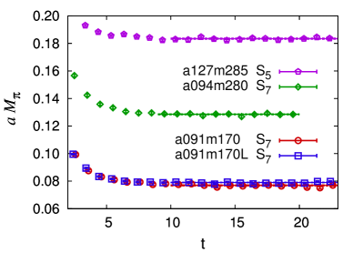
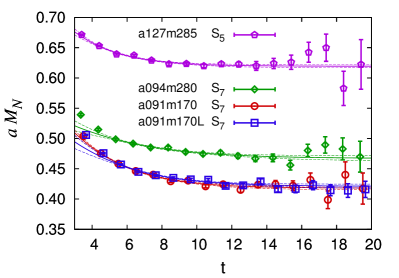
Figure 1: Data for the the effective mass of the pion (left) and the nucleon (nucleon) obtained using 2-state fits to the zero-momentum two-point correlation functions. The ensemble ID and smearing size are specified in the labels. The 2-state fits to the nucleon are made with our “best” value of $\mathop{t_{\rm min}}\nolimits$ described in the text.

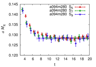
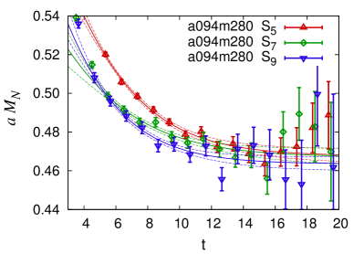
Figure 2: Comparison of the effective mass of the pion (left) and the nucleon (right) obtained using 2-state fits to the zero-momentum two-point correlation functions on the $a094m280$ ensemble for three different smearings, $S_{5}S_{5}$, $S_{7}S_{7}$ and, $S_{9}S_{9}$. The 2-state fits to the nucleon are made with our “best” value of $\mathop{t_{\rm min}}\nolimits$ described in the text.

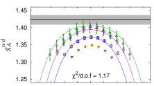
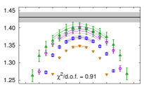
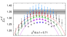
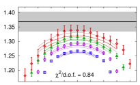
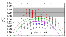
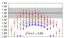
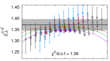
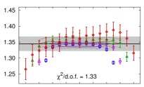
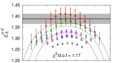
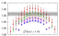
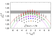
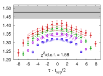
Figure 3: Two- (left) and three-state (right) fits to $g_{A}^{u-d}$ from the 6 simulations on the 4 ensembles as described in the text. (Left) Data not included in the fits based on $\tau_{\rm skip}^{\rm best}$ are shown in grey. (Right) Lines showing the fits are limited to points fit.

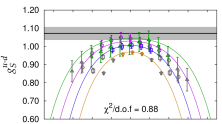
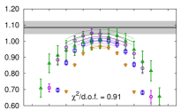
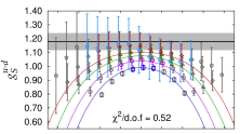
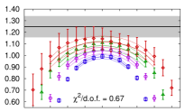
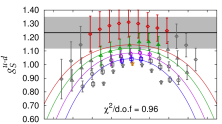
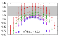
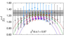
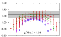
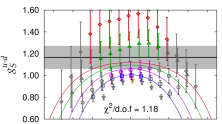
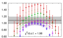
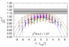
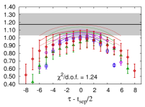
Figure 4: Two- (left) and three-state (right) fits to $g_{S}^{u-d}$ from the 6 simulations on the 4 ensembles as described in the text. (Left) Data not included in the fits based on $\tau_{\rm skip}^{\rm best}$ are shown in grey. (Right) Lines showing the fits are limited to points fit.

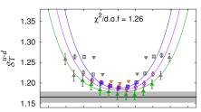
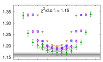
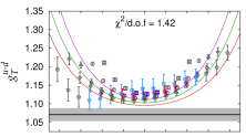
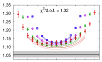
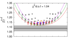
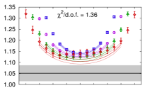
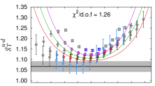
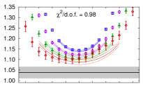
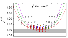
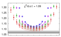
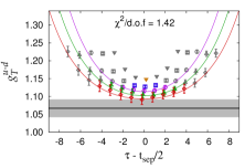
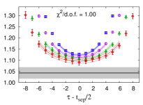
Figure 5: Two- (left) and three-state (right) fits to $g_{T}^{u-d}$ from the 6 simulations on the 4 ensembles as described in the text. (Left) Data not included in the fits based on $\tau_{\rm skip}^{\rm best}$ are shown in grey. (Right) Lines showing the fits are limited to points fit.

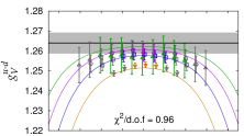
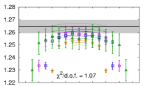
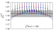
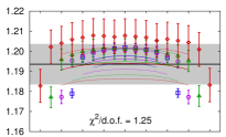
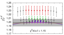
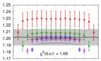
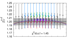
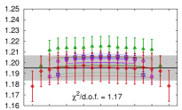
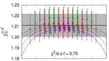
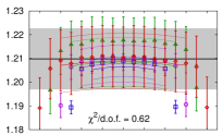
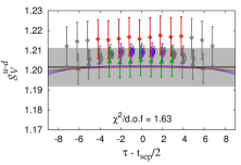
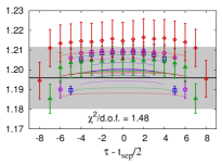
Figure 6: Two- (left) and three-state (right) fits to $g_{V}^{u-d}$ from the 6 simulations on the 4 ensembles as described in the text. (Left) Data not included in the fits based on $\tau_{\rm skip}^{\rm best}$ are shown in grey. (Right) Lines showing the fits are limited to points fit.

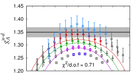
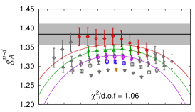
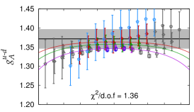
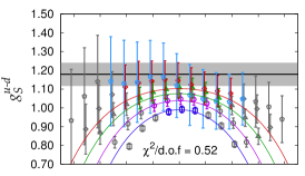
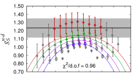
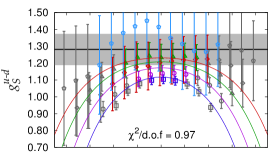
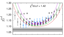
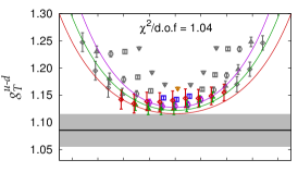
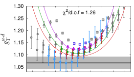
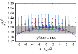
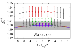
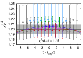
Figure 7: Comparison of the 2-state fits to the data for $g_{A,S,T,V}^{u-d}$ for the three calculations on the $a094m280$ ensemble with different smearing parameter $\sigma$. Each row shows results for the $S_{5}S_{5}$ (left) $S_{7}S_{7}$ (middle) and $S_{9}S_{9}$ (right) calculations.

III Fits and Excited-state contamination

To understand and control excited-state contamination we present analyses using 2-, 3- and 4-state fits to the two-point functions and 2- and 3-state fits to the three-point functions. We find that to get reliable estimates of the masses $M_{i}$ and amplitudes ${\cal A}_{i}$ for the first $N$ states we need to include $N+1$ states in the fit to the two-point function. For this reason, we analyze the correlation functions with the following combinations $\{\mathop{N_{\rm 2pt}}\nolimits,\mathop{N_{\rm 3pt}}\nolimits\}=\{2,2\}$, $\{3,2\}$, $\{4,2\}$, $\{3,3\}$ and $\{4,3\}$ where the first (second) value is the number of states included in fits to the two-point (three-point) functions. In each case, the methodology employed in the analysis is the same except that when using three and higher state fits to two-point functions we introduce non-uniform priors.

In each fit, to understand and quantify the excited-state contamination, there are three parameters that we optimize: (i) the starting time slice $\mathop{t_{\rm min}}\nolimits$ used in fits to the two-point data; (ii) the number of time slices $\mathop{\tau_{\rm skip}}\nolimits$, adjacent to the source and sink, skipped in fits to the three-point functions; and (iii) the values of $\mathop{t_{\rm sep}}\nolimits$ at which data are collected used in the fits. The final values of these parameters, chosen on the basis of the $\chi^{2}$ and the stability of the fits, represent a compromise between statistical precision and reducing excited-state contamination. In general, we reduce the value of $\mathop{t_{\rm min}}\nolimits$ and $\mathop{\tau_{\rm skip}}\nolimits$ and enlarge the number of $\mathop{t_{\rm sep}}\nolimits$ values included when increasing the number of states in the fit ansatz. For example, we set $\mathop{t_{\rm min}}\nolimits=2$ in 4-state fits to the two-point functions. Even then, in the case of 4-state fits, only about eight points contribute to determining the six excited-state parameters since the plateau in the effective-mass plot starts at $t\approx 10$ as shown in Figs. 1 and 2.

Our focus is on obtaining estimates for the charges in the $\mathop{t_{\rm sep}}\nolimits\to\infty$ limit for the six calculations labeled as $\{C1,C2,C5,C6,C7,C8\}$ in Table 2. Two overall caveats that will be made explicit at appropriate places are: the statistics in the case of the $a091m170L$ ensemble ($C8$) are insufficient as the auto-correlations between configurations are large. Similarly, the errors in the data for $g_{S}$ are much larger than for $g_{A,T}$, consequently the fits used to extract $g_{S}$ are much less stable. In all cases, the fits and the error analysis presented here are based on using the full covariance matrix.

III.1 Analysis using 2-state fits

The selection of the best combination of $\mathop{t_{\rm min}}\nolimits$, $\mathop{\tau_{\rm skip}}\nolimits$ and $\mathop{t_{\rm sep}}\nolimits$ for the quoted results using 2-state fits was carried out as follows:

• Step 1: Fits to the two-point correlators using the full covariance matrix for different values of $\mathop{t_{\rm min}}\nolimits$ were made. The best value minimizing the correlated $\chi^{2}/{\rm d.o.f.}$ was determined to be $\mathop{t_{\rm min}^{\rm best}}\nolimits=\{4,5,5,4,4,5\}$ for the six calculations.

• Step 2: Using these values of $\mathop{t_{\rm min}^{\rm best}}\nolimits$, we determined the four parameters $aM_{0}$, $aM_{1}$, ${\cal A}_{0}^{2}$ and ${\cal A}_{1}^{2}$. Then, 2-state fits to the three-point data were performed for the three sets of $\mathop{t_{\rm sep}}\nolimits$, labeled A, B and C, in Table 3. Since the pattern of excited-state contamination is different in the various charges, the best set was determined separately for each charge. Our final results are based on Fit B for the scalar and vector charges, and Fit C for the axial and tensor charges as discussed below.

• Step 3: Repeat Step 2 for the three cases $\mathop{\tau_{\rm skip}}\nolimits=\{1,2\},\ \{2,3\}$ and $\{3,4\}$ for the $a\approx\{0.127,0.09\}$ ensembles, respectively. All three cases gave overlapping results. For our quoted 2-state results, we use $\{3,4\}$ as it removes the most points adjacent to the source and sink that have the largest excited-state contamination.

• Step 4: To quantify the dependence on $\mathop{t_{\rm min}}\nolimits$, we repeat Steps 1–3 for $\mathop{t_{\rm min}}\nolimits=\mathop{t_{\rm min}^{\rm best}}\nolimits\pm 1$.

Results for $aM_{0}$, $aM_{1}$, ${\cal A}_{0}^{2}$ and ${\cal A}_{1}^{2}$ for $\mathop{t_{\rm min}^{\rm best}}\nolimits$ and $\mathop{t_{\rm min}^{\rm best}}\nolimits\pm 1$ are given in Table 4. Results for the three matrix elements for our best choice of $\mathop{t_{\rm min}}\nolimits$, $\mathop{\tau_{\rm skip}}\nolimits$ and $\mathop{t_{\rm sep}}\nolimits$ are given in Table 5. Estimates of the ratios of the unrenormalized charges, $g_{A,S,T}/g_{V}$, are given in Table 6.

	Fit A	Fit B	Fit C
$a127m285$	$\{8,10,12\}$	$\{8,10,12,14\}$	$\{10,12,14\}$
$a094m280$,
$a091m170$,	$\{10,12,14\}$	$\{10,12,14,16\}$	$\{12,14,16\}$
$a091m170L$

Table 3: The three fits, defined by the values of $\mathop{t_{\rm sep}}\nolimits$ used in the 2-state fit, investigated to quantify the stability of the $\mathop{t_{\rm sep}}\nolimits\to\infty$ estimate.

ID	Type	Fit Range	$aM_{0}$	$aM_{1}$	${\cal A}_{0}^{2}$	${\cal A}_{1}^{2}$	${\cal A}_{1}^{2}/{\cal A}_{0}^{2}$	$\chi^{2}/$d.o.f.
	$S_{5}S_{5}$	3–20	0.6206(20)	1.099(45)	3.51(7)e-08	2.19(11)e-08	0.624(28)	1.26
$a127m285$	$S_{5}S_{5}$	4–20	0.6193(27)	1.048(71)	3.46(10)e-08	1.98(23)e-08	0.572(55)	1.31
	$S_{5}S_{5}$	5–20	0.6181(31)	0.980(85)	3.40(13)e-08	1.66(29)e-08	0.487(77)	1.36
	$S_{5}S_{5}$	4–20	0.4721(25)	0.851(28)	2.86(9)e-08	3.41(13)e-08	1.195(41)	1.33
$a094m280$	$S_{5}S_{5}$	5–20	0.4676(37)	0.776(39)	2.67(15)e-08	2.92(16)e-08	1.096(57)	0.96
	$S_{5}S_{5}$	6–20	0.4643(51)	0.724(50)	2.51(22)e-08	2.62(19)e-08	1.042(90)	0.91
	$S_{7}S_{7}$	4–20	0.4711(30)	0.864(65)	5.55(21)e-10	3.91(40)e-10	0.705(59)	1.08
$a094m280$	$S_{7}S_{7}$	5–20	0.4670(48)	0.739(77)	5.19(40)e-10	3.02(29)e-10	0.583(66)	0.9
	$S_{7}S_{7}$	6–20	0.4654(65)	0.70(10)	5.04(58)e-10	2.86(37)e-10	0.568(92)	0.97
	$S_{9}S_{9}$	3–20	0.4672(25)	0.925(47)	4.52(13)e-12	3.83(24)e-12	0.847(45)	0.94
$a094m280$	$S_{9}S_{9}$	4–20	0.4635(37)	0.809(65)	4.29(21)e-12	3.02(28)e-12	0.705(58)	0.73
	$S_{9}S_{9}$	5–20	0.4642(40)	0.83(10)	4.33(24)e-12	3.21(75)e-12	0.74(15)	0.78
	$S_{7}S_{7}$	3–22	0.4209(24)	0.859(29)	4.67(12)e-10	4.90(14)e-10	1.050(27)	1.42
$a091m170$	$S_{7}S_{7}$	4–22	0.4180(30)	0.802(37)	4.50(16)e-10	4.41(22)e-10	0.981(43)	1.25
	$S_{7}S_{7}$	5–22	0.4183(32)	0.808(55)	4.51(18)e-10	4.49(55)e-10	1.00(10)	1.34
	$S_{7}S_{7}$	4–22	0.4252(19)	0.895(44)	4.87(10)e-10	4.80(44)e-10	0.985(76)	1.75
$a091m170L$	$S_{7}S_{7}$	5–22	0.4210(36)	0.755(72)	4.59(24)e-10	3.35(40)e-10	0.730(62)	1.46
	$S_{7}S_{7}$	6–22	0.410(11)	0.584(79)	3.73(85)e-10	2.82(50)e-10	0.76(30)	1.1

Table 4: Estimates of the nucleon masses $M_{0}$ and $M_{1}$ and the amplitudes ${\cal A}_{0}$ and ${\cal A}_{1}$ extracted from fits to the two-point correlation functions data using the 2-state ansatz given in (7). For the $a094m280$ ensemble, we give the estimates from the three runs with different smearing parameters described in Table 2. The notation $S_{5}S_{5}$ labels a nucleon correlation function with source and sink constructed using smearing parameter $\sigma=5$. We give estimates for three different fit ranges $\mathop{t_{\rm min}^{\rm best}}\nolimits$ and $\mathop{t_{\rm min}^{\rm best}}\nolimits\pm 1$, expressed in lattice units, as described in the text.

		Axial			Scalar			Tensor
ID	Type	$\langle 0|\mathcal{O}_{A}|0\rangle$	$\langle 0|\mathcal{O}_{A}|1\rangle$	$\langle 1|\mathcal{O}_{A}|1\rangle$	$\langle 0|\mathcal{O}_{S}|0\rangle$	$\langle 0|\mathcal{O}_{S}|1\rangle$	$\langle 1|\mathcal{O}_{S}|1\rangle$	$\langle 0|\mathcal{O}_{T}|0\rangle$	$\langle 0|\mathcal{O}_{T}|1\rangle$	$\langle 1|\mathcal{O}_{T}|1\rangle$
a127m285	$S_{5}S_{5}$	1.423(14)	-0.179(21)	-0.9(2.4)	1.07(4)	-0.35(4)	0.6(1.1)	1.166(13)	0.182(16)	-0.2(1.2)
a094m280	$S_{5}S_{5}$	1.349(19)	-0.130(20)	0.6(0.7)	1.18(6)	-0.42(5)	1.0(0.8)	1.071(17)	0.157(15)	0.7(4)
a094m280	$S_{7}S_{7}$	1.384(28)	-0.111(36)	0.3(1.3)	1.23(12)	-0.52(12)	1.4(1.7)	1.085(30)	0.221(36)	0.0(0.8)
a094m280	$S_{9}S_{9}$	1.372(25)	-0.026(39)	-0.4(2.5)	1.28(9)	-0.42(9)	-0.6(3.3)	1.067(25)	0.276(28)	0.6(1.6)
a091m170	$S_{7}S_{7}$	1.388(23)	-0.133(33)	-2.1(2.6)	1.17(11)	-0.48(7)	0.1(3.9)	1.091(20)	0.154(22)	-0.2(1.7)
a091m170L	$S_{7}S_{7}$	1.401(20)	-0.118(26)	-1.0(2.4)	1.15(8)	-0.44(8)	1.4(2.2)	1.067(25)	0.235(23)	0.5(8)

Table 5: Estimates of the three matrix elements $\langle 0|\mathcal{O}_{\Gamma}|0\rangle$, $\langle 0|\mathcal{O}_{\Gamma}|1\rangle$, $\langle 1|\mathcal{O}_{\Gamma}|1\rangle$ for the three isovector operators obtained using the 2-state fit to the three-point correlators with our “best” choices of $\mathop{t_{\rm min}}\nolimits$, $\mathop{t_{\rm sep}}\nolimits$ and $\mathop{\tau_{\rm skip}}\nolimits$.

ID	Type	$g_{A}/g_{V}$	$g_{S}/g_{V}$	$g_{T}/g_{V}$
a127m285	$S_{5}S_{5}$	1.125(11)	0.848(27)	0.922(12)
a094m280	$S_{5}S_{5}$	1.130(17)	0.987(50)	0.897(15)
a094m280	$S_{7}S_{7}$	1.154(24)	1.030(95)	0.906(27)
a094m280	$S_{9}S_{9}$	1.143(22)	1.068(76)	0.889(22)
a091m170	$S_{7}S_{7}$	1.146(21)	0.963(84)	0.901(16)
a091m170L	$S_{7}S_{7}$	1.166(18)	0.960(69)	0.888(21)

Table 6: Estimates of the ratios of the unrenormalized isovector charges $g_{A,S,T}/g_{V}$ with our “best” choices of $\mathop{t_{\rm min}}\nolimits$, $\mathop{t_{\rm sep}}\nolimits$ and $\mathop{\tau_{\rm skip}}\nolimits$ in the 2-state fits.

The quality of the data for the two-point functions on the four ensembles is illustrated by plotting the effective mass,

$$aM_{N,eff}(t+0.5)=\ln\frac{C^{\rm 2pt}(t)}{C^{\rm 2pt}(t+1)}\,,$$ (11)

for the pion and the nucleon in Fig. 1. As expected, the signal in the pion does not degrade with $t$, whereas that for the proton becomes noisy by $t=20$, with 1–2 $\sigma$ fluctuations in $M_{N,eff}$ apparent already at $t\approx 16$. The onset of a plateau indicates that the ground-state pion mass can be extracted using 1-state fits to data at $t>10$. In practice, the ground state mass is largely determined from the region $10\lesssim t\lesssim 16$, while the excited state masses and amplitudes are determined from the region $t\lesssim 10$. The value of $\mathop{t_{\rm min}}\nolimits$ is, therefore, adjusted depending on the number of states included in the fit.

To assess the statistical quality of the data, the auto-correlation function was calculated using two quantities that have reasonable estimates on each configuration: (i) the pion two-point correlator at $t=14$ and (ii) the three-point correlation function at the midpoint in $\tau$ for $\mathop{t_{\rm sep}}\nolimits=12$. Autocorrelations increase as $M_{\pi}$ or $a$ is decreased or $L$ is increased. In particular, the data from the $a091m170L$ ensemble showed significant auto-correlations. In this case, the 467 configurations consist of four streams with roughly 170, 100, 100 and 100 configurations. These are too few to even determine the auto-correlation time reliably. For the other ensembles, the auto-correlation function falls to $<1/e$ by 1–2 configurations, and binning the data by a factor of two did not change the Jackknife error estimates. Our overall conclusion is that much larger statistics are needed to get reliable error estimates on the $a091m170L$ ensemble and it is very likely that the quoted $1\sigma$ errors for this ensemble, evaluated without taking into account auto-correlations, are underestimates.

To exhibit the dependence of the two-point correlation functions on the smearing size given by $\sigma$, we show a comparison of the effective mass for the pion and the nucleon for the $S_{5}S_{5}$, $S_{7}S_{7}$ and $S_{9}S_{9}$ correlators on the $a094m280$ ensemble in Fig. 2. We find that the errors in the effective-mass data (and in the raw two-point functions) increase with the smearing size $\sigma$ for both the pion and the proton. The onset of the plateau in both states, however, occurs at earlier times with larger $\sigma$. Thus, the relative reduction in the excited-state contamination in the correlation functions with larger smearing $\sigma$ has to be balanced against the increase in statistical noise. Based on these trends on the $a094m280$ ensemble, our compromise choice for the three ensembles at $a\approx 0.09$ fm is $\sigma=7$ and for the $a127m285$ ensemble it is $\sigma=5$. In physical units, this choice corresponds to setting the size of the smearing parameter $\sigma\approx 0.65$ fm.

Our final estimates for the four parameters $aM_{0}$, $aM_{1}$, ${\cal A}_{0}^{2}$, ${\cal A}_{1}^{2}$ and the ratio ${\cal A}_{1}^{2}/{\cal A}_{0}^{2}$ for three values of $\mathop{t_{\rm min}}\nolimits$ are given in Table 4. In addition to minimizing $\chi^{2}/{\rm d.o.f.}$, we required $\lesssim 1\sigma$ stability in the value of $M_{0}$ under the variation $\mathop{t_{\rm min}^{\rm best}}\nolimits\pm 1$ as criteria for choosing our best $\mathop{t_{\rm min}}\nolimits$. With the selected $\mathop{t_{\rm min}^{\rm best}}\nolimits=\{4,5,5,4,4,5\}$, we find that $aM_{1}$ is also consistent within $2\sigma$ except on the $a091m170L$ ensemble which, as stated above, requires much higher statistics.

To illustrate the three-point function data and the size of excited-state contamination, we plot an “effective” charge,

$$g_{\Gamma}^{\text{eff}}(t_{\text{sep}},\tau)=\frac{C^{\text{3pt}}_{\Gamma}(t_{\text{sep}},\tau)}{C^{\text{2pt}}_{\text{fit}}(t_{\text{sep}})}\,,$$ (12)

i.e., the ratio of the three-point function to the n-state fit that describes the two-point function. This ratio converges to $g_{\Gamma}$ as the time separations $\tau$ and $t_{\text{sep}}-\tau$ become large provided the fit to the two-point function, $C^{\text{2pt}}_{\text{fit}}(t_{\text{sep}})$, gives the ground state. Our methodology for taking into account excited-state contamination and obtaining estimates of the charges from data with $\mathop{t_{\rm sep}}\nolimits$ in the limited range 1–1.5 fm is described next.

The data and the 2-state fits to the ratio of the three- to two-point functions using our best choice of $\mathop{t_{\rm min}}\nolimits$, $\mathop{t_{\rm sep}}\nolimits$ and $\mathop{\tau_{\rm skip}}\nolimits$ are shown in Figs. 3,  4,  5 and 6 for the four isovector charges. In the right panels of these figures, we show the 3-state fits, discussed in Sec. III.2, to facilitate comparison.

The magnitude of the excited-state contamination as a function of $\mathop{t_{\rm sep}}\nolimits$ and the smearing parameter $\sigma$ is different for the four charges. The dependence on $\sigma$ is exhibited in Fig. 7 for the $S_{5}S_{5}$, $S_{7}S_{7}$ and $S_{9}S_{9}$ calculations on the $a094m280$ ensemble. In $g_{A}^{u-d}$, the magnitude of the excited-state contamination, measured as the difference between the data at the central values of $\tau$ for $\mathop{t_{\rm sep}}\nolimits=12$ (about 1 fm) and the $\mathop{t_{\rm sep}}\nolimits\to\infty$ estimate, is about 10%, 5% and 3% for the $S_{5}S_{5}$, $S_{7}S_{7}$ and $S_{9}S_{9}$ calculations, respectively. The pattern in $g_{S}^{u-d}$ is similar, however, the reduction in the contamination with $\sigma$ is smaller. For $g_{T}^{u-d}$, the overall variation with $\mathop{t_{\rm sep}}\nolimits$ and between the three estimates is $\leq 5\%$. The vector charge $g_{V}^{u-d}$ shows insignificant excited-state contamination and no detectable dependence on $\sigma$. On the other hand, the errors in individual data points increase with the smearing $\sigma$ for all four charges.

We use the data with the three values of the smearing $\sigma$ on the $a094m280$ ensemble to test whether the 2-state fit gives equally reliable $\mathop{t_{\rm sep}}\nolimits\to\infty$ estimates in spite of differences in the excited-state contamination. We find that the three estimates are consistent within $1\sigma$ for all four charges as shown in Fig. 7. However, because the magnitude of the excited-state effect is different in the four charges $g_{A,S,T,V}$, we do not uniformly use the same set of values of $\mathop{t_{\rm sep}}\nolimits$ in our final 2-state fit, but tune them for each case.

Based on the data shown in these figures and on the results of the fits with our best choices of the input fit parameters given in Tables 5 and 6, we evaluate below the excited-state effect in each of the charges and the efficacy of the 2-state fit in providing $\mathop{t_{\rm sep}}\nolimits\to\infty$ estimates.

• The data for the axial charge $g_{A}^{u-d}$ shown in Fig. 3 converges to the $\mathop{t_{\rm sep}}\nolimits\to\infty$ value from below and at the central values of $\tau$ show up to 10% variation with $\mathop{t_{\rm sep}}\nolimits$ due to excited-state contamination. We, therefore, use Fit C based on data with the larger values of $\mathop{t_{\rm sep}}\nolimits$. In all but the $a127m285$ case, the data at $\mathop{t_{\rm sep}}\nolimits\gtrsim 16$ lies above the result of the fit. The errors in these data, however, are large. Thus, to confirm the $\mathop{t_{\rm sep}\to\infty}\nolimits$ estimate, requires additional high precision data for $\mathop{t_{\rm sep}}\nolimits\geq 16$.

  The data with $S_{9}S_{9}$ correlators on the $a094m280$ ensemble show the least excited-state effect: the estimates at the central values of $\tau$ show only a tiny increase with $\mathop{t_{\rm sep}}\nolimits$ and their error bands overlap. As a result, the matrix elements $\langle 0|\mathcal{O}_{T}|1\rangle$ and $\langle 1|\mathcal{O}_{T}|1\rangle$, given in Table 5, are poorly determined.

• The data for the scalar charge $g_{S}^{u-d}$ have larger uncertainty so we choose Fit B to include all the data except that with $\mathop{t_{\rm sep}}\nolimits=8$ and $18$ on the $a094m280$ ensemble. As shown in Fig. 4, the 2-state fits again converge from below, the three estimates from the $a094m280$ ensemble are consistent within $1\sigma$ as shown in Fig. 7, and the estimates from the $a091m170$ and $a091m170L$ ensembles overlap.

• The data for the tensor charge $g_{T}^{u-d}$ show small excited-state contamination and converge to the $\mathop{t_{\rm sep}}\nolimits\to\infty$ estimate from above. Fits to the the data for $g_{T}^{u-d}$ are the most stable and all the fits give consistent estimates. We choose Fit C for the final estimates. These estimates agree with those from Fit B, and the $\chi^{2}/{\rm d.o.f.}$ of both fits are also consistent.

• The data for the vector charge $g_{V}^{u-d}$ show little variation with $\tau$ or $\mathop{t_{\rm sep}}\nolimits$. The excited-state contamination is highly suppressed because $g_{V}^{u-d}$ is associated with a conserved charge at $O(a)$. As a result, statistical fluctuations in the data stand out. Note that the error estimates in $g_{V}^{u-d}$ from the fits are comparable to the 1–2% variance in individual data points at the largest $\mathop{t_{\rm sep}}\nolimits$. Only the $S_{7}S_{7}$ data with $\mathop{t_{\rm sep}}\nolimits=16$ on the $a094m280$ ensemble deviate by about $2\sigma$ from the result of the fit.

In the next section, we extend the analysis to include up to 4-states in fits to the two-point function data and 3-states in fits to the three-point functions to evaluate the stability of estimates obtained using 2-state fits.

III.2 Analysis using 3-state fits

In this section, we investigate the stability of the $\mathop{t_{\rm sep}\to\infty}\nolimits$ estimates from 2-state fits by increasing the number of states kept in the fits to the two- and three-point function data. The additional features introduced into the analysis, over and above those discussed in Sec III.1 for the 2-state fits, are:

• The two-point function data were analyzed using 3- and 4-state fits. In fits with more than two states, the excited state masses and amplitudes are, in many cases, ill-determined. The fits were stabilized by carrying out an empirical Bayesian analysis with Gaussian priors for both the mass gaps and the amplitudes of the excited states Lepage et al. (2002); Chen et al. (2004).

• With more fit parameters, the values of $\mathop{t_{\rm min}}\nolimits$ and $\mathop{\tau_{\rm skip}}\nolimits$ were reduced to increase the number of data points included in the fits to both two- and three-point functions. The results with the final choices of these parameters for various fits are listed in Tables 7 and 8.

• Data with $\mathop{t_{\rm sep}}\nolimits=8,\ 10,\ 12$ and 14 were used for all four charges in fits to the three-point functions on the $a127m285$ ensemble and with $\mathop{t_{\rm sep}}\nolimits=10,\ 12,\ 14$ and 16 for the three $a\approx 0.09$ fm ensembles.

The priors for the 3- and 4-state fits to the two-point function data were determined empirically as follows:

• The ground state mass and amplitude are very well constrained by the plateau in the effective mass for $t\gtrsim 10$. Thus, no non-trivial priors were needed or used for determining ${\cal A}_{0}$ and $M_{0}$.

• Results for ${\cal A}_{1}$ and $M_{1}$ obtained from 2-state fits without priors were used to guide the selection of their priors in 3-state fits. The width was chosen to be large but consistent with the requirement that the $1\sigma$ bands for $r_{i}\equiv({\cal A}_{i}^{2}/{\cal A}_{0}^{2})$ and the $\Delta M_{i}\equiv(M_{i}-M_{i-1})$ are positive. These priors did not need any subsequent changes.

• Results for $r_{2}$ and $\Delta M_{2}$ from the 3-state fit were used as priors in the 4-state fits along with ${\cal A}_{3}^{2}/{\cal A}_{0}^{2}=1\pm 0.6$ and $\Delta M_{3}\equiv M_{3}-M_{2}=0.4\pm 0.3$. The output estimates were used as the new central values of these two sets of priors without decreasing their width and the fits were carried out a second time to get the final estimates.

• In all cases except for the $a091m170L$ data, the final results are close to the central value chosen for the priors for both the 3- and 4-state fits.

• The quoted errors are obtained using a single elimination jackknife procedure with the full covariance matrix and constant priors.

• The augmented $\chi^{2}/{\rm d.o.f.}$ is given by the standard correlated $\chi^{2}$ plus the square of the deviation of the parameter from the prior normalized by the width. This is then divided by the number of degrees of freedom calculated ignoring the priors.

	$\mathcal{A}_{0}^{2}$	$aM_{0}$	$r_{1}$	$a\Delta M_{1}$	$r_{2}$	$a\Delta M_{2}$	$r_{3}$	$a\Delta M_{3}$	$\chi^{2}/\text{d.o.f}$
	$a127m285$ Smearing $\sigma=5$
Priors			$0.6(3)$	$0.35(20)$	$0.65(35)$	$0.8(4)$	$1.0(5)$	$0.4(3)$
{2,4–20}	3.46(11)$\times 10^{-8}$	$0.619(3)$	$0.57(6)$	$0.43(7)$					$1.31$
{3,2–20}	3.42(10)$\times 10^{-8}$	$0.619(2)$	$0.49(4)$	$0.38(5)$	$0.71(13)$	$0.91(10)$			$1.02$
{4,2–20}	3.43(9)$\times 10^{-8}$	$0.619(2)$	$0.54(4)$	$0.40(5)$	$0.45(6)$	$1.06(9)$	$0.77(13)$	$0.49(2)$	$1.07$
	$a094m280$ Smearing $\sigma=5$
Priors			$1.0(5)$	$0.23(12)$	$1.3(6)$	$0.6(3)$	$0.8(5)$	$0.4(3)$
{2,5–20}	2.67(15)$\times 10^{-8}$	$0.468(4)$	$1.10(6)$	$0.31(4)$					$0.96$
{3,3–20}	2.49(18)$\times 10^{-8}$	$0.464(4)$	$0.90(10)$	$0.24(4)$	$1.61(24)$	$0.62(7)$			$0.71$
{4,3–20}	2.45(24)$\times 10^{-8}$	$0.463(5)$	$0.92(11)$	$0.23(5)$	$1.22(17)$	$0.58(10)$	$0.73(12)$	$0.41(4)$	$0.69$
	$a094m280$ Smearing $\sigma=7$
Priors			$0.6(3)$	$0.23(12)$	$0.8(6)$	$0.6(3)$	$0.6(4)$	$0.4(3)$
{2,5–20}	5.19(40)$\times 10^{-10}$	$0.467(5)$	$0.58(7)$	$0.27(7)$					$0.90$
{3,3–20}	5.03(39)$\times 10^{-10}$	$0.466(4)$	$0.48(9)$	$0.22(5)$	$1.05(21)$	$0.64(8)$			$0.74$
{4,3–20}	4.97(45)$\times 10^{-10}$	$0.465(5)$	$0.50(9)$	$0.21(6)$	$0.77(16)$	$0.62(8)$	$0.58(9)$	$0.40(3)$	$0.73$
	$a094m280$ Smearing $\sigma=9$
Priors			$0.6(3)$	$0.23(12)$	$0.8(6)$	$0.6(3)$	$0.6(4)$	$0.4(3)$
{2,4–20}	4.29(21)$\times 10^{-12}$	$0.464(4)$	$0.71(6)$	$0.35(6)$					$0.73$
{3,2–20}	4.16(20)$\times 10^{-12}$	$0.462(3)$	$0.55(8)$	$0.27(4)$	$1.08(16)$	$0.71(10)$			$0.67$
{4,2–20}	4.11(22)$\times 10^{-12}$	$0.461(4)$	$0.56(8)$	$0.26(5)$	$0.67(10)$	$0.64(11)$	$0.57(9)$	$0.41(3)$	$0.65$
	$a091m170$ Smearing $\sigma=7$
Priors			$0.8(5)$	$0.30(15)$	$1.0(6)$	$0.7(5)$	$1.0(5)$	$0.4(3)$
{2,4–22}	4.49(16)$\times 10^{-10}$	$0.418(3)$	$0.98(4)$	$0.38(3)$					$1.25$
{3,2–22}	4.42(16)$\times 10^{-10}$	$0.417(3)$	$0.88(6)$	$0.35(3)$	$1.22(20)$	$0.91(13)$			$1.05$
{4,2–22}	4.44(17)$\times 10^{-10}$	$0.417(3)$	$0.91(6)$	$0.36(4)$	$0.72(18)$	$0.91(20)$	$0.87(16)$	$0.45(2)$	$1.05$
	$a091m170L$ Smearing $\sigma=7$
Priors			$0.5(3)$	$0.21(5)$	$1.0(9)$	$0.6(4)$	$0.8(6)$	$0.30(25)$
{2,5–22}	4.59(24)$\times 10^{-10}$	$0.421(4)$	$0.73(6)$	$0.33(7)$					$1.46$
{3,2–22}	4.22(23)$\times 10^{-10}$	$0.417(3)$	$0.45(10)$	$0.19(2)$	$1.30(8)$	$0.54(4)$			$1.00$
{4,2–22}	4.20(25)$\times 10^{-10}$	$0.417(3)$	$0.44(10)$	$0.18(2)$	$0.74(5)$	$0.47(4)$	$0.60(4)$	$0.19(5)$	$1.03$

Table 7: Results of 2-, 3- and 4-state fits to the two-point correlation data for the six calculations. The first column specifies the parameters, {$N_{\text{2pt}}$, $t_{\text{min}}$– $t_{\text{max}}$}, where $N_{\text{2pt}}$ number of states used in the fits to the two-point correlators, and $[t_{\text{min}},t_{\text{max}}]$ is the fit interval in lattice units. The following columns give the nucleon ground state amplitude $\mathcal{A}_{0}^{2}$ and mass $aM_{0}$, followed by the ratio of the excited state amplitudes $r_{i}=(\mathcal{A}_{i}/\mathcal{A}_{0})^{2}$, and a mass gaps $a\Delta M_{i}=a(M_{i}-M_{i-1})$. For each ensemble, the first row gives the values of the priors used in the final fits.

ID	Type	Fit	$\mathop{t_{\rm sep}}\nolimits$	$g_{A}^{u-d}$	$g_{S}^{u-d}$	$g_{T}^{u-d}$	$g_{V}^{u-d}$
a127m285	$S_{5}S_{5}$	{2,2,3,4–20}	{10,12,14}	$1.423(14)$		$1.166(13)$
		{2,2,3,4–20}	{8,10,12,14}		$1.07(4)$		$1.264(5)$
		{4,2,3,2–20}	{8,10,12,14}	$1.413(12)$	$1.08(3)$	$1.153(11)$	$1.265(5)$
		{4,3,3,2–20}	{8,10,12,14}	$1.431(29)$	$1.09(4)$	$1.160(12)$	$1.264(7)$
		{4,$3^{\ast}$,3,2–20}	{8,10,12,14}	$1.431(15)$	$1.09(4)$	$1.160(10)$	$1.264(5)$
a094m280	$S_{5}S_{5}$	{2,2,4,5–20}	{12,14,16}	$1.349(19)$		$1.071(17)$
		{2,2,4,5–20}	{10,12,14,16}		$1.18(6)$		$1.194(8)$
		{4,2,4,3–20}	{10,12,14,16}	$1.365(34)$	$1.30(13)$	$1.025(40)$	$1.197(9)$
		{4,3,2,3–20}	{10,12,14,16}	$1.369(36)$	$1.31(15)$	$1.066(23)$	$1.208(17)$
		{4,$3^{\ast}$,2,3–20}	{10,12,14,16}	$1.369(34)$	$1.25(9)$	$1.057(19)$	$1.194(10)$
a094m280	$S_{7}S_{7}$	{2,2,4,5–20}	{12,14,16}	$1.384(28)$		$1.085(30)$
		{2,2,4,5–20}	{10,12,14,16}		$1.23(12)$		$1.199(10)$
		{4,2,4,3–20}	{10,12,14,16}	$1.398(38)$	$1.34(17)$	$1.015(61)$	$1.201(11)$
		{4,3,2,3–20}	{10,12,14,16}	$1.390(40)$	$1.35(21)$	$1.077(34)$	$1.243(28)$
		{4,$3^{\ast}$,2,3–20}	{10,12,14,16}	$1.381(32)$	$1.20(12)$	$1.051(36)$	$1.202(12)$
a094m280	$S_{9}S_{9}$	{2,2,4,4–20}	{12,14,16}	$1.372(25)$		$1.067(25)$
		{2,2,4,4–20}	{10,12,14,16}		$1.28(9)$		$1.200(10)$
		{4,2,4,2–20}	{10,12,14,16}	$1.355(20)$	$1.36(11)$	$1.028(34)$	$1.199(11)$
		{4,3,2,2–20}	{10,12,14,16}	$1.345(30)$	$1.39(18)$	$1.038(28)$	$1.195(38)$
		{4,$3^{\ast}$,2,2–20}	{10,12,14,16}	$1.345(23)$	$1.25(11)$	$1.038(28)$	$1.195(12)$
a091m170	$S_{7}S_{7}$	{2,2,4,4–22}	{12,14,16}	$1.388(23)$		$1.091(20)$
		{2,2,4,4–22}	{10,12,14,16}		$1.17(10)$		$1.211(11)$
		{4,2,4,2–22}	{10,12,14,16}	$1.370(16)$	$1.19(11)$	$1.068(16)$	$1.211(11)$
		{4,3,2,2–22}	{10,12,14,16}	$1.363(17)$	$1.09(11)$	$1.070(15)$	$1.210(13)$
		{4,$3^{\ast}$,2,2–22}	{10,12,14,16}	$1.363(17)$	$1.09(11)$	$1.070(15)$	$1.210(13)$
a091m170L	$S_{7}S_{7}$	{2,2,4,5–22}	{12,14,16}	$1.401(20)$		$1.067(25)$
		{2,2,4,5–22}	{10,12,14,16}		$1.15(8)$		$1.202(10)$
		{4,2,4,2–22}	{10,12,14,16}	$1.464(31)$	$1.37(13)$	$0.962(38)$	$1.202(15)$
		{4,3,2,2–22}	{10,12,14,16}	$1.480(46)$	$0.78(22)$	$1.032(30)$	$1.196(23)$
		{4,$3^{\ast}$,2,2–22}	{10,12,14,16}	$1.477(38)$	$1.18(14)$	$1.043(26)$	$1.196(16)$

Table 8: Estimates of the bare isovector charges $g_{A,S,T,V}$ for four choices of $\{N_{\text{2pt}},N_{\text{3pt}},\mathop{\tau_{\rm skip}}\nolimits,\mathop{t_{\rm min}}\nolimits-\mathop{t_{\rm max}}\nolimits\}$, where $\{N_{\text{2pt}},N_{\text{3pt}}\}$ are the number of states kept in fits to the two- and three-point functions, respectively. The $N_{\text{3pt}}=3^{\ast}$ fit is a 3-states fit with $\langle 2\lvert\mathcal{O}_{\Gamma}\rvert 2\rangle=0$. Note that the choice of $t_{\text{min}}=3$ is the same as in Table 7 except for the $a127m285$ data. Our final estimates are given in the last row corresponding to the {4,$3^{\ast}$} fit.

ID	Type	$g_{A}/g_{V}$	$g_{S}/g_{V}$	$g_{T}/g_{V}$
a127m285	$S_{5}S_{5}$	1.132(11)	0.858(31)	0.918(8)
a094m280	$S_{5}S_{5}$	1.147(31)	1.046(77)	0.885(17)
a094m280	$S_{7}S_{7}$	1.149(26)	0.994(99)	0.875(32)
a094m280	$S_{9}S_{9}$	1.125(19)	1.048(89)	0.869(23)
a091m170	$S_{7}S_{7}$	1.127(16)	0.898(88)	0.884(13)
a091m170L	$S_{7}S_{7}$	1.235(35)	0.983(118)	0.872(23)

Table 9: Estimates of the ratios of the unrenormalized isovector charges $g_{A,S,T}/g_{V}$ from the {4,$3^{\ast}$} fits with our “best” choices of $\mathop{t_{\rm min}}\nolimits$, $\mathop{t_{\rm sep}}\nolimits$ and $\mathop{\tau_{\rm skip}}\nolimits$.

ID	Type	$\langle 0\lvert\mathcal{O}_{A}\rvert 1\rangle$	$\langle 0\lvert\mathcal{O}_{S}\rvert 1\rangle$	$\langle 0\lvert\mathcal{O}_{T}\rvert 1\rangle$	$\langle 0\lvert\mathcal{O}_{V}\rvert 1\rangle$	$\langle 1\lvert\mathcal{O}_{A}\rvert 1\rangle$	$\langle 1\lvert\mathcal{O}_{S}\rvert 1\rangle$	$\langle 1\lvert\mathcal{O}_{T}\rvert 1\rangle$	$\langle 1\lvert\mathcal{O}_{V}\rvert 1\rangle$
a127m285	$S_{5}S_{5}$	$-0.179(21)$		$0.182(16)$		$-0.9(2.4)$		$-0.2(1.2)$
			$-0.35(4)$		$-0.014(2)$		$0.6(1.1)$		$0.80(34)$
		$-0.172(18)$	$-0.37(4)$	$0.210(15)$	$-0.015(2)$	$0.75(48)$	$0.8(9)$	$0.42(27)$	$0.87(28)$
		$-0.295(58)$	$-0.45(15)$	$0.167(40)$	$-0.014(6)$	$1.5(3.0)$	$1.8(1.4)$	$0.54(86)$	$0.86(55)$
		$-0.295(57)$	$-0.45(15)$	$0.166(47)$	$-0.014(6)$	$1.46(54)$	$1.8(1.4)$	$0.54(41)$	$0.86(28)$
a094m280	$S_{5}S_{5}$	$-0.130(20)$		$0.157(15)$		$0.62(69)$		$0.70(40)$
			$-0.42(5)$		$-0.006(1)$		$1.0(8)$		$1.35(14)$
		$-0.139(34)$	$-0.57(13)$	$0.224(46)$	$-0.008(2)$	$1.10(22)$	$1.4(6)$	$0.71(12)$	$1.29(9)$
		$-0.136(36)$	$-0.42(8)$	$0.141(25)$	$-0.005(2)$	$1.00(41)$	$-0.2(2.0)$	$0.64(34)$	$0.99(32)$
		$-0.136(36)$	$-0.42(8)$	$0.140(25)$	$-0.005(2)$	$1.01(25)$	$1.1(6)$	$0.84(12)$	$1.29(10)$
a094m280	$S_{7}S_{7}$	$-0.111(36)$		$0.221(36)$		$0.3(1.3)$		$0.03(80)$
			$-0.52(12)$		$-0.003(3)$		$1.4(1.7)$		$1.25(26)$
		$-0.150(48)$	$-0.69(20)$	$0.347(81)$	$-0.004(3)$	$1.09(42)$	$1.8(1.4)$	$0.37(26)$	$1.21(19)$
		$-0.111(47)$	$-0.39(15)$	$0.236(44)$	$-0.004(3)$	$0.72(92)$	$-3.2(4.4)$	$-0.24(80)$	$-0.10(92)$
		$-0.113(47)$	$-0.41(15)$	$0.231(43)$	$-0.004(3)$	$1.03(42)$	$1.8(1.3)$	$0.63(25)$	$1.18(20)$
a094m280	$S_{9}S_{9}$	$-0.026(39)$		$0.276(28)$		$-0.4(2.5)$		$0.6(1.6)$
			$-0.42(9)$		$-0.004(3)$		$-0.6(3.3)$		$1.51(49)$
		$-0.003(34)$	$-0.53(13)$	$0.346(52)$	$-0.005(3)$	$1.04(45)$	$0.4(2.3)$	$0.50(39)$	$1.41(33)$
		$0.048(49)$	$-0.20(15)$	$0.287(36)$	$-0.003(3)$	$0.7(1.3)$	$-7.9(7.5)$	$0.70(41)$	$1.4(2.0)$
		$0.048(49)$	$-0.21(15)$	$0.287(36)$	$-0.003(3)$	$0.71(50)$	$-0.1(2.1)$	$0.70(37)$	$1.45(34)$
a091m170	$S_{7}S_{7}$	$-0.133(33)$		$0.154(22)$		$-2.1(2.6)$		$-0.2(1.7)$
			$-0.48(7)$		$-0.006(2)$		$0.1(3.5)$		$1.11(46)$
		$-0.142(25)$	$-0.51(8)$	$0.187(18)$	$-0.006(2)$	$0.65(63)$	$0.3(3.4)$	$0.73(37)$	$1.13(39)$
		$-0.117(25)$	$-0.35(7)$	$0.180(16)$	$-0.006(2)$	$0.60(62)$	$1.3(3.5)$	$0.73(37)$	$1.16(44)$
		$-0.117(25)$	$-0.35(7)$	$0.180(16)$	$-0.006(2)$	$0.60(62)$	$1.3(3.5)$	$0.73(37)$	$1.16(44)$
a091m170L	$S_{7}S_{7}$	$-0.118(26)$		$0.235(23)$		$-1.0(2.4)$		$0.54(84)$
			$-0.44(8)$		$-0.002(2)$		$1.4(2.2)$		$1.26(34)$
		$-0.222(44)$	$-0.87(16)$	$0.474(54)$	$-0.003(3)$	$0.98(31)$	$2.7(1.4)$	$-0.17(33)$	$1.25(20)$
		$-0.258(71)$	$-0.38(21)$	$0.202(48)$	$0.004(4)$	$0.96(83)$	$12.7(6.8)$	$0.86(53)$	$1.25(46)$
		$-0.259(71)$	$-0.37(21)$	$0.208(48)$	$0.004(4)$	$1.02(35)$	$2.5(1.5)$	$0.51(24)$	$1.26(20)$

Table 10: Estimates of the matrix elements $\langle 0\lvert\mathcal{O}_{\Gamma}\rvert 1\rangle$ and $\langle 0\lvert\mathcal{O}_{\Gamma}\rvert 1\rangle$ for the three isovector operators. Results for the four choices of the fit parameters $\{N_{2pt},N_{3pt},\mathop{\tau_{\rm skip}}\nolimits,\mathop{t_{\rm min}}\nolimits-\mathop{t_{\rm max}}\nolimits\}$ are arranged as defined in Table 8 with the the final estimates from the $\{N_{2pt},N_{3pt}\}=\{4,3^{\ast}\}$ fit given in the last row.

ID	Type	$\langle 0\lvert\mathcal{O}_{A}\rvert 2\rangle$	$\langle 0\lvert\mathcal{O}_{S}\rvert 2\rangle$	$\langle 0\lvert\mathcal{O}_{T}\rvert 2\rangle$	$\langle 0\lvert\mathcal{O}_{V}\rvert 2\rangle$	$\langle 1\lvert\mathcal{O}_{A}\rvert 2\rangle$	$\langle 1\lvert\mathcal{O}_{S}\rvert 2\rangle$	$\langle 1\lvert\mathcal{O}_{T}\rvert 2\rangle$	$\langle 1\lvert\mathcal{O}_{V}\rvert 2\rangle$
a127m285	$S_{5}S_{5}$	$0.97(66)$	$1.2(1.4)$	$0.03(37)$	$-0.012(75)$	$-3.7(4.7)$	$-11.3(11.3)$	$3.7(3.4)$	$0.01(62)$
		$0.97(66)$	$1.2(1.4)$	$0.03(37)$	$-0.012(90)$	$-3.7(4.7)$	$-11.3(11.3)$	$3.7(3.4)$	$0.02(79)$
a094m280	$S_{5}S_{5}$	$-0.02(2)$	$-0.18(7)$	$0.09(2)$	$-0.007(3)$	$0.21(23)$	$-0.38(44)$	$0.28(14)$	$-0.01(2)$
		$-0.02(2)$	$-0.18(7)$	$0.09(2)$	$-0.007(3)$	$0.21(23)$	$-0.36(44)$	$0.29(14)$	$-0.01(2)$
a094m280	$S_{7}S_{7}$	$-0.05(4)$	$-0.36(10)$	$0.13(3)$	$-0.006(5)$	$0.34(42)$	$0.40(97)$	$0.18(26)$	$-0.01(3)$
		$-0.05(4)$	$-0.37(10)$	$0.14(3)$	$-0.006(5)$	$0.35(43)$	$0.55(99)$	$0.19(25)$	$-0.01(3)$
a094m280	$S_{9}S_{9}$	$-0.13(5)$	$-0.39(15)$	$0.07(4)$	$-0.008(6)$	$0.48(63)$	$-0.7(1.8)$	$0.51(45)$	$0.06(6)$
		$-0.13(5)$	$-0.38(15)$	$0.07(4)$	$-0.008(6)$	$0.48(63)$	$-0.7(1.8)$	$0.51(45)$	$0.06(6)$
a091m170	$S_{7}S_{7}$	$0.11(6)$	$-0.09(16)$	$0.12(4)$	$0.006(8)$	$-0.4(1.2)$	$-3.8(4.0)$	$1.0(1.1)$	$-0.18(12)$
		$0.11(6)$	$-0.09(16)$	$0.12(4)$	$0.006(8)$	$-0.4(1.2)$	$-3.8(4.0)$	$1.0(1.1)$	$-0.18(12)$
a091m170L	$S_{7}S_{7}$	$0.01(4)$	$-0.20(12)$	$0.18(3)$	$-0.013(4)$	$0.03(25)$	$-1.55(87)$	$0.12(18)$	$0.03(2)$
		$0.01(4)$	$-0.18(12)$	$0.18(3)$	$-0.013(4)$	$0.03(24)$	$-1.74(89)$	$0.11(18)$	$0.03(2)$

Table 11: Estimates of the matrix elements $\langle 0\lvert\mathcal{O}_{\Gamma}\rvert 2\rangle$ and $\langle 1\lvert\mathcal{O}_{\Gamma}\rvert 2\rangle$ for the three isovector operators obtained using 3-state fits. The two rows gives results for the $N_{\text{3pt}}=3$ and $N_{\text{3pt}}=3^{\ast}$ fits. Estimates of the matrix element $\langle 2\lvert\mathcal{O}_{\Gamma}\rvert 2\rangle$ from the $N_{\text{3pt}}=3$ fits are not presented as they are ill-determined.

The results of fits to the two-point function data are shown in Table 7 for the three cases, 2-, 3- and 4-state fits using our best choices of $\mathop{t_{\rm min}}\nolimits$. The results of the 2-state fits are reproduced from Table 4. Overall, the results presented in Tables 7 exhibit the following behavior:

• The 2-, 3- and 4-state fits to the two-point data on the $a127m285$ ensemble data are very stable and the central values show little variation with changes in $\mathop{t_{\rm min}}\nolimits$ and/or the number of states. Similarly, the estimates of all four charges are stable within $1\sigma$. Fits to the data from the $a094m280$ and $a091m170$ ensembles were also stable but the variation in the results was larger.

• Estimates of the ground-state mass $M_{0}$ and the mass gap $\Delta M_{1}$ obtained from the 3-state and 4-state fits are essentially identical. Even estimates of $\Delta M_{2}$ are consistent.

• All three ratios of amplitudes, $r_{i}$, decrease with the smearing size $\sigma$ between $\sigma=5$ and $7$ and then are essentially flat between $\sigma=7$ and $9$ on the $a094m280$ ensemble. Note also that the amplitudes for $S_{9}S_{9}$ are essentially the same for $\mathop{t_{\rm min}}\nolimits=2$ and 3.

• The 3- and 4-state fits to the two-point data on the $a091m170L$ ensemble are sensitive to the choice of the priors, their widths and $\mathop{t_{\rm min}}\nolimits$. Furthermore, for any choice of fit parameters for the two-point functions, the results for the four charges are sensitive to the choice of $\mathop{\tau_{\rm skip}}\nolimits$. As remarked in Sec. III.1, we attribute this sensitivity to low statistics in the $a091m170L$ calculation and reiterate that the quoted errors are underestimates since the auto-correlations between configurations, that are significant, have not been taken into account.

With 3- and 4-state fits to the two-point data in hand we carried out three analyses to estimate the isovector charges: $\{\mathop{N_{\rm 2pt}}\nolimits,\mathop{N_{\rm 3pt}}\nolimits\}=\{4,2\}$, $\{4,3\}$ and $\{4,3^{\ast}\}$. The $\{\mathop{N_{\rm 2pt}}\nolimits,\mathop{N_{\rm 3pt}}\nolimits\}=\{4,3^{\ast}\}$ is a 3-state fit with $\langle 2|\mathcal{O}_{\Gamma}|2\rangle$ set to zero. The reason for this additional analysis is that $\langle 2|\mathcal{O}_{\Gamma}|2\rangle$ is essentially undetermined in the $\{\mathop{N_{\rm 2pt}}\nolimits,\mathop{N_{\rm 3pt}}\nolimits\}=\{4,3\}$ fits. This is because (i) the contribution of $\langle 2|\mathcal{O}_{\Gamma}|2\rangle$ for any of the four charges is suppressed by at least $e^{-6}$ relative to $\langle 1|\mathcal{O}_{\Gamma}|1\rangle$ as can be deduced from Eq. (8) and the data in Table 7; (ii) the three matrix elements, $\langle 0|\mathcal{O}_{\Gamma}|0\rangle$, $\langle 1|\mathcal{O}_{\Gamma}|1\rangle$, and $\langle 2|\mathcal{O}_{\Gamma}|2\rangle$ are only sensitive to $\mathop{t_{\rm sep}}\nolimits$, and the data at the four values of $\mathop{t_{\rm sep}}\nolimits$ overlap within $1\sigma$. Thus, three matrix elements cannot be determined reliably from overlapping data at four values of $\mathop{t_{\rm sep}}\nolimits$. (iii) Even $\langle 1|\mathcal{O}_{\Gamma}|1\rangle$ is poorly determined as shown by the data in Table 10.

We find that setting $\langle 2|\mathcal{O}_{\Gamma}|2\rangle=0$ leads to a significant improvement over the unconstrained $\{\mathop{N_{\rm 2pt}}\nolimits,\mathop{N_{\rm 3pt}}\nolimits\}=\{4,3\}$ fit. Thus, our final unrenormalized estimates for the four charges are taken from the $\{\mathop{N_{\rm 2pt}}\nolimits,\mathop{N_{\rm 3pt}}\nolimits\}=\{4,3^{\ast}\}$ fits and given in Tab. 8. These fits are shown in the right panels of Figs. 3, 4, 5 and 6. Estimates for the matrix elements $\langle 0|\mathcal{O}_{\Gamma}|1\rangle$, $\langle 1|\mathcal{O}_{\Gamma}|1\rangle$, $\langle 0|\mathcal{O}_{\Gamma}|2\rangle$ and $\langle 1|\mathcal{O}_{\Gamma}|2\rangle$ are given in Tabs. 10 and 11.

The data in Table 8 show that estimates for the four charges from the four analyses, $\{\mathop{N_{\rm 2pt}}\nolimits,\mathop{N_{\rm 3pt}}\nolimits\}=\{2,2\},\{4,2\}$, $\{4,3\}$ and $\{4,3^{\ast}\}$, are consistent. Based on this stability and the small size of the variation in estimates under changes in the values of $\mathop{t_{\rm min}}\nolimits$ and $\mathop{\tau_{\rm skip}}\nolimits$ that have been investigated, we conclude that estimates for $g_{A,T,V}$ can be obtained with $O(3\%)$ uncertainty from $\{\mathop{N_{\rm 2pt}}\nolimits,\mathop{N_{\rm 3pt}}\nolimits\}=\{4,3^{\ast}\}$ fits to data comprising $O(10^{5})$ measurements. Our statistical tests also indicate that this estimate of the number of measurements required will increase as the lattice spacing and the pion mass are decreased. The data in Figs. 3, 4, 5 and 6 further indicate that increasing the statistics to $O(10^{6})$ measurements on each ensemble will lead to results for $g_{A,T,V}$ with $O(1\%)$ uncertainty. This factor of ten increase in statistics will have to come primarily from increasing the number of independent gauge configurations analyzed since the $O(100)$ measurements per configuration that we have made in this study were shown to be optimal in Ref. Yoon et al. (2016).

Our final results for the isovector charges, using bare estimates from the $\{\mathop{N_{\rm 2pt}}\nolimits,\mathop{N_{\rm 3pt}}\nolimits\}=\{4,3^{\ast}\}$ fits given in Tables 8 and 9 and renormalized using the factors given in Table 12, are given in Tables 13 and 14.

IV Renormalization Constants

We calculated the renormalization constants $Z_{\Gamma}$ for the isovector quark bilinear operators $\overline{u}\Gamma d$ on the lattice using the non-perturbative RI-sMOM scheme Martinelli et al. (1995); Sturm et al. (2009). Details of the procedure for calculating the three-point functions and the renormalization conditions used are given in Ref. Bhattacharya et al. (2014). In short, in the RI-sMOM scheme we require the projected amputated three-point function $\Lambda^{\text{R}}$, renormalized at the scale $q^{2}$, to satisfy the condition

$$\left.\Lambda^{\text{R}}_{\Gamma}(p_{a},p_{b})\right|_{p_{a}^{2}=p_{b}^{2}=q^{2}}=1=\\ \left.\left(Z_{\psi}^{-1}Z_{\Gamma}~{}\Lambda^{\text{PA}}_{\Gamma}(p_{i},p_{f})\right)\right|_{p_{a}^{2}=p_{b}^{2}=q^{2}},$$ (13)

where $p_{a}^{\mu}$ and $p_{b}^{\mu}$ are the 4-momenta in the two fermion legs, $q^{\mu}=p_{b}^{\mu}-p_{a}^{\mu}$ and they satisfy the kinematic constraint $p_{a}^{2}=p_{b}^{2}=q^{2}$. Here $\Lambda^{\text{PA}}$ is the projected amputated three-point function discussed below and $Z_{\psi}$ is the wavefunction renormalization constant defined by

$$\left.(Z_{\psi})^{-1}\frac{i}{12}\operatorname{Tr}\left(\frac{/\!\!\!{p}\langle S(p)\rangle^{-1}}{p^{2}}\right)\right|_{p^{2}=q^{2}}=1\,.$$ (14)

It is obtained from the momentum space quark propagator $S(p)$ calculated on lattices fixed to the Landau gauge defined as the maximum of the sum of the trace of the gauge links. The notation $\langle\cdots\rangle$ denotes ensemble average. The projected amputated three-point function is

$$\Lambda^{\text{PA}}_{\Gamma}(p_{a},p_{b})=\frac{1}{12}\operatorname{Tr}\Big{(}P_{\Gamma}\Lambda^{\text{A}}_{\Gamma}(p_{a},p_{b})\Big{)},$$ (15)

where the amputated vertex $\Lambda^{\text{A}}_{\Gamma}(p_{a},p_{b})$ is defined as

$$\Lambda^{\text{A}}_{\Gamma}(p_{a},p_{b})=\\ \langle\langle S(p_{a})\rangle^{-1}S(p_{a})\,\Gamma\,(\gamma_{5}S^{\dagger}(p_{b})\gamma_{5})\langle(\gamma_{5}S^{\dagger}(p_{b})\gamma_{5})\rangle^{-1}\rangle.$$ (16)

The projector $P_{\Gamma}$ for the RI-sMOM scheme is $I$ (scalar), $(q_{\mu}/{q^{2}})/\!\!\!{q}$ (vector), $(q_{\mu}/{q^{2}})\gamma_{5}/\!\!\!{q}$ (axial-vector) or $(i/12)\gamma_{[\mu}\gamma_{\nu]}$ (tensor). In $\Lambda^{\text{PA}}_{\Gamma}(p_{a},p_{b})$, lattice artifacts due to the breaking of the rotational symmetry to $O(4)$ can induce dependence on the momenta $p_{a}$ and $p_{b}$ in addition to that on $q^{2}$. This systematic is significant in our data as discussed below.

We analyzed 132, 100 and 100 configurations on the three ensembles, $a127m285$, $a094m280$ and $a091m170$, respectively, to get estimates at the three distinct values of $a$ and $M_{\pi}$ simulated. With this sample size, we find that the statistical errors in the data are much smaller than the systematics discussed below.

Operationally, we first translate the lattice data, $Z_{\Gamma}^{\rm RI-sMOM}(p_{a},p_{b},q^{2})$, to the $\overline{\text{MS}}$ scheme at $2$ GeV. This is done by matching estimates at a given squared momentum transfer $q^{2}$ to the $\overline{\text{MS}}$ scheme in the continuum at the same $q^{2}$ (horizontal matching) using 2-loop perturbative relations expressed in terms of the coupling constant $\alpha_{\overline{\text{MS}}}(q^{2})$ Gracey (2011). These results in the $\overline{\text{MS}}$ scheme are then run to $2$ GeV using the 3-loop anomalous dimension relations for the scalar and tensor bilinears Gracey (2000); Olive et al. (2014) and labeled $Z_{\Gamma}(p_{a},p_{b},q^{2})$.

The calculation of $\alpha_{\overline{\text{MS}}}(q^{2})$ was carried out as follows. Starting with the 5-flavor $\alpha_{\overline{\text{MS}}}(M_{Z}=91.1876\ {\rm GeV})=0.1185$, we used the 4-loop expression in ${\overline{\text{MS}}}$ scheme Chetyrkin et al. (2000) to run to the bottom quark threshold at $m_{b}=4.18$ GeV, and then to $m_{c}=1.275$ GeV using the 4-flavor evolution. This 4-flavor result was converted to 3-flavor at this scale and then run to the final desired $q^{2}$ using the 3-flavor evolution.

Ideally, after removing the dependence on $p_{a}$ and $p_{b}$ from $Z_{\Gamma}(p_{a},p_{b},q^{2})$, one expects a window, $\eta\Lambda_{\rm QCD}\ll q\ll\xi\pi/a$, in which the data for the renormalized $Z(\overline{\text{MS}},2\ {\rm GeV})$ are independent of $q$; that is, at sufficiently small values of the lattice spacing $a$, the data should show a plateau versus $q$. The lower cutoff $\eta\Lambda_{\rm QCD}$ is dictated by nonperturbative effects and the upper cutoff $\xi\pi/a$ by discretization effects. Here $\eta$ and $\xi$ are, a priori, unknown dimensionless numbers of $O(1)$ that depend on the lattice action and the gauge-link smearing procedure.

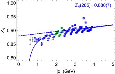
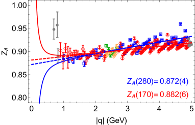
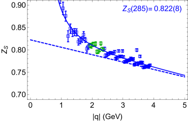
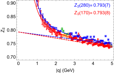
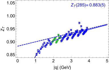
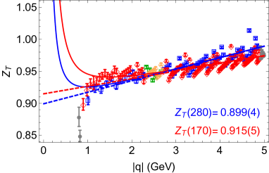
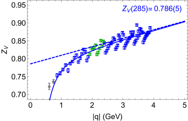
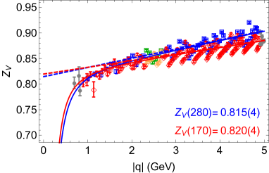
Figure 8: Data for the renormalization constants $Z_{A}$, $Z_{S}$, $Z_{T}$ and $Z_{V}$ in the $\overline{\text{MS}}$ scheme at $2\mathop{\rm GeV}\nolimits$, keeping only points that minimizes $\sum_{\mu}(p^{a}_{\mu})^{4}+\sum_{\mu}(p^{b}_{\mu})^{4}$ for each $q^{2}$ as described in the text. Estimates from the $a127m285$ ensemble are shown as blue squares in the left panels. The data points used in estimating the $Z$’s in method B are shown as green squares. The right panel shows estimates for the $a094m280$ (blue squares) and the $a091m170$ (red diamonds) ensembles. The data points included in the estimate of $Z$ using method B are shown as green squares ($a094m280$) and yellow diamonds ($a091m170$). The results given in the labels are from method A using the fit ansatz $c/q^{2}+Z+d_{1}q$ as described in the text. The fit is shown by the solid blue (red) line and the result $Z+d_{1}q$ by the dashed blue (red) line.

The data, shown in Figs. 8, 9, 10 and 11, do not exhibit such a window in which they are independent of $q^{2}$, as needed for a unique determination of the $Z_{\Gamma}$ and the ratios $Z_{\Gamma}/Z_{V}$. The lattice artifacts are much larger than the statistical errors. The four main systematics contributing to the lack of such a window and the resulting uncertainty in the extraction of the renormalization constants are (i) breaking of the Euclidean $O(4)$ rotational symmetry to the hypercubic group, because of which different combinations of momenta with the same $q^{2}$ give different results in the RI-sMOM scheme; (ii) discretization errors at large $q^{2}$ other than these $O(4)$ breaking effects; (iii) nonperturbative effects at small $q^{2}$; and (iv) truncation errors in the perturbative matching to the $\overline{\text{MS}}$ scheme and the running to $2\mathop{\rm GeV}\nolimits$.

To reduce these systematics, we estimate $Z_{\Gamma}$ using three methods. In methods A and B, to reduce artifacts due to the breaking of rotational symmetry on the lattice, we only keep points that minimize $\sum_{\mu}[(p_{a}^{\mu})^{4}+(p_{b}^{\mu})^{4}]$ when there are multiple combinations of momenta $p_{a}^{\mu}$ and $p_{b}^{\mu}$ that have the same $q^{2}$. These points, after conversion to the $\overline{\text{MS}}$ scheme at $\mu=2\mathop{\rm GeV}\nolimits$ are shown in Figs. 8 and 9 as a function of $\sqrt{q^{2}}$, the momentum flowing in all three legs in the RI-sMOM scheme. Using this subset of the data, the first two estimates are obtained as follows:

Method A: We fit the data in the $\overline{\text{MS}}$ scheme at $\mu=2\mathop{\rm GeV}\nolimits$ for $q^{2}>0.85$ GeV² using the ansatz $c/q^{2}+Z_{\Gamma}+d_{1}q$. The first term, $c/q^{2}$, is introduced to account for non-perturbative artifacts and the third, $d_{1}q$, for discretization errors. These fits are shown in Figs. 8 and 9. In these figures, the data from the ensembles $a094m280$ and $a091m170$ are plotted together to show that possible dependence on the pion mass is much smaller than the statistical errors or the lattice artifacts.

Method B: We choose the estimate for $Z_{\Gamma}$ by taking an average over data points about $q^{2}=\Lambda/a$, where $\Lambda=3$ GeV is a scale chosen to be small enough to avoid discretization effects, large enough to avoid non-perturbative effects, and above which perturbation theory is expected to be reasonably well-behaved. With this choice, both $qa\to 0$ and $\Lambda/q\to 0$ in the continuum limit as desired. In our simulations, the values of $q^{2}$ are $4.7$ and $6.4$ GeV² for the $a=0.127$ and $0.09$ fm ensembles, respectively. Thus, the value from method B and the error in it is taken to be the mean and the standard deviation of the data over the ranges 3.7–5.7 and 5.4–7.4 GeV² for the ensembles at $a=0.127$ and $0.09$ fm, respectively.

Method C: We first isolate the $O(4)$ breaking artifacts in the data, $Z(p_{a},p_{b},q^{2})$, by using a fit. This was done in Refs. Boucaud et al. (2003, 2006) for different kinematics ($p_{a}=p_{b}$) with terms up to $O(p^{4})$. We generalize that ansatz to our kinematics:

$$\begin{split}Z_{\Gamma}(p_{a},p_{b},q^{2})&=Z_{\Gamma}^{0}(q^{2})\\ &\quad+a^{4}\sum_{i=0}^{2}c^{(1)}_{i}p_{S}^{[4,i]}+a^{2}\sum_{i=0}^{2}c^{(2)}_{i}\frac{p_{S}^{[4,i]}}{q^{2}}\\ &\quad+a^{4}\sum_{i=0}^{3}c^{(3)}_{i}\frac{p_{S}^{[6,i]}}{q^{2}}+a^{4}\sum_{\begin{subarray}{c}i,j=0\\ i\leq j\end{subarray}}^{2}c^{(4)}_{ij}\frac{p_{S}^{[4,i]}p_{S}^{[4,j]}}{q^{4}}\\ &\quad+a^{4}\sum_{\begin{subarray}{c}i,j=0\\ i\leq j\end{subarray}}^{1}c^{(5)}_{ij}\frac{p_{A}^{[4,i]}p_{A}^{[4,j]}}{q^{4}},\end{split}$$ (17)

where

$$p_{S,A}^{[n,i]}=\sum_{\mu}\left[(p_{a}^{\mu})^{n-i}(p_{b}^{\mu})^{i}\pm(p_{a}^{\mu})^{i}(p_{b}^{\mu})^{n-i}\right]\,.$$ (18)

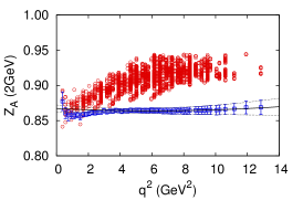
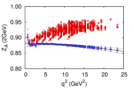
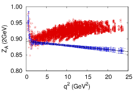
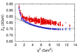
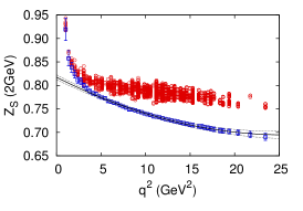
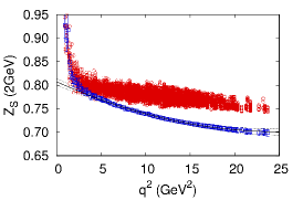
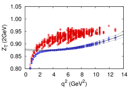
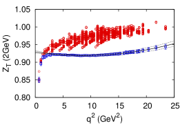
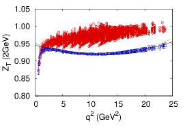
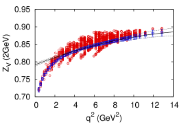
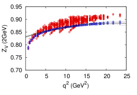
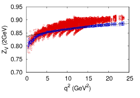
Figure 10: Data for the renormalization constants $Z_{A}$, $Z_{S}$, $Z_{T}$ and $Z_{V}$ in the $\overline{\text{MS}}$ scheme at $2\mathop{\rm GeV}\nolimits$ using method C described in the text. All the data from the $a127m285$ (left) $a094m280$ (middle) and $a091m170$ (right) ensembles are shown as red circles. The data after correcting for the rotational symmetry breaking are shown as blue squares. The corrected data (blue squares) are then fit using the ansatz $Z+e_{2}q^{2}+e_{4}q^{4}$ to estimate the $Z$. The fit is shown by the solid black line.

Here, for each tensor structure $\Gamma$, the $Z_{\Gamma}^{0}(q^{2})$ are independent parameters for each $q^{2}$, and the nineteen $c_{i}$, whose $q^{2}$ dependence is ignored, parameterize terms that break the $O(4)$ symmetry. Also, only $Z_{\Gamma}(p_{a},p_{b},q^{2})$ with momenta satisfying $\{|p_{a}^{\mu}|,|p_{b}^{\mu}|,|q^{\mu}|\}\leq\pi/(2a)$ are included in the fit. The $Z_{0}(q^{2})$, after conversion to the $\overline{\text{MS}}$ scheme at $\mu=2\mathop{\rm GeV}\nolimits$, are then fit over the ranges $q^{2}=$4–16 ($a127m285$) and $q^{2}=$4–25 GeV² ($a094m280$ and $a091m170$) using the ansatz $Z+e_{2}q^{2}+e_{4}q^{4}$ to extract the desired $Z_{\Gamma}$. We show all the data, $Z_{\Gamma}(p_{a},p_{b},q^{2})$, as red circles in Figs 10 and 11 and the $Z_{\Gamma}^{0}(q^{2})$ as blue squares. The final fit, along with the error band, is shown by the black lines. The data have been analyzed to obtain both $Z_{\Gamma}$ and the ratios $Z_{\Gamma}/Z_{V}$, and their final values are collected in Table 12.

On comparing the raw data presented in Figs 10 and 11 (red circles), we find the data for the ratios $Z_{\Gamma}/Z_{V}$ show a smaller spread, presumably because some of the systematics cancel. As a result, the errors in estimates from all three methods, shown in Table 12, are smaller with the ratio method. Also, in all three methods, the region of $q^{2}$ that contributes to the fits is consistent with the general requirement that $\eta\Lambda_{\rm QCD}\ll q\ll\zeta\pi/a$ with $\eta$ and $\zeta$ of $O(1)$ to avoid both non-perturbative and discretization artifacts.

ID	Method	$Z_{A}$	$Z_{S}$	$Z_{T}$	$Z_{V}$	$Z_{A}/Z_{V}$	$Z_{S}/Z_{V}$	$Z_{T}/Z_{V}$
$a127m285$	A	0.880(7)	0.822(8)	0.883(5)	0.786(5)	1.119(6)	1.024(7)	1.111(4)
$a127m285$	B	0.891(9)	0.807(7)	0.908(9)	0.829(13)	1.075(8)	0.974(13)	1.096(8)
$a127m285$	C	0.867(5)	0.839(10)	0.877(5)	0.791(4)	1.094(5)	1.052(12)	1.107(5)
$a127m285$	AV	0.879(12)	0.823(16)	0.889(16)	0.802(22)	1.096(22)	1.017(39)	1.105(7)
$a094m280$	A	0.872(4)	0.793(7)	0.899(4)	0.815(4)	1.081(3)	0.976(4)	1.106(3)
$a094m280$	B	0.901(9)	0.790(9)	0.947(8)	0.855(10)	1.054(4)	0.924(8)	1.106(5)
$a094m280$	C	0.889(4)	0.817(5)	0.929(4)	0.831(3)	1.060(4)	0.978(5)	1.116(4)
$a094m280$	AV	0.887(15)	0.800(14)	0.925(24)	0.834(20)	1.065(14)	0.959(27)	1.109(5)
$a091m170$	A	0.882(6)	0.793(8)	0.915(5)	0.820(4)	1.086(4)	0.973(6)	1.116(3)
$a091m170$	B	0.899(6)	0.779(4)	0.949(6)	0.850(8)	1.058(4)	0.916(7)	1.116(5)
$a091m170$	C	0.892(4)	0.807(7)	0.946(5)	0.837(3)	1.065(4)	0.961(7)	1.129(4)
$a091m170$	AV	0.891(9)	0.793(14)	0.937(17)	0.836(15)	1.070(14)	0.950(29)	1.120(6)

Table 12: The renormalization constants $Z_{A}$, $Z_{S}$, $Z_{T}$, $Z_{V}$ and the ratios $Z_{A}/Z_{V}$, $Z_{S}/Z_{V}$ and $Z_{T}/Z_{V}$ in the $\overline{\text{MS}}$ scheme at $2\mathop{\rm GeV}\nolimits$ at the two values of the lattice spacings. For each ensemble, the three rows give estimates for the three methods (A, B and C) described in the text. The fourth row gives the mean (AV) with the error given by the larger of the two—half the spread or the largest statistical error. This average value is taken to be our final estimate of the renormalization factor.

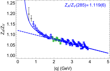
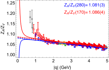
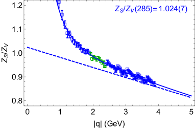
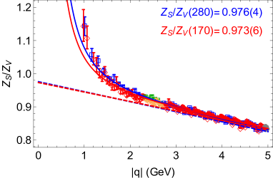
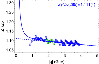
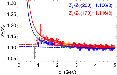
Figure 9: Data for the ratios of renormalization constants $Z_{A}/Z_{V}$, $Z_{S}/Z_{V}$ and $Z_{T}/Z_{V}$ in the $\overline{\text{MS}}$ scheme at $2\mathop{\rm GeV}\nolimits$ on the $a127m285$ (left) and the $a094m280$ and $a091m170$ (right) ensembles. The rest is the same as in Fig. 8.

The estimates from the three methods, given in Tab 12, have different systematics. For example, as shown in Figs  8, 9, 10 and 11, the variation with $q^{2}$, in many cases, is large. Nevertheless, the estimates from the three methods agree to within about 2%. We, therefore, take the average of the three as our final estimate. To assign a conservative error, we use half the spread between the three estimates since it is larger than the statistical errors.

We also point out that the 2-loop perturbative expression for the matching of $Z_{T}$ between the RI-sMOM scheme and the $\overline{\text{MS}}$ scheme is badly behaved over the range of $q^{2}$ investigated. For example, the successive terms in the loop expansion are $1+0.0052+0.0159$ at $q^{2}=4$ GeV² ($\alpha^{\overline{MS}}=0.2979$) and $1+0.0037+0.0078$ at $q^{2}=25$ GeV² ($\alpha^{\overline{MS}}=0.2041$) using the matching expressions given in Ref. Gracey (2011). We, therefore, take the average of the two 2-loop correction at $q^{2}=4$ and $25$ GeV², 0.012, as a systematic error in the estimates of $Z_{T}$ due to truncation errors. The series for $Z_{S}$ at $q^{2}=4$ GeV², $1-0.0157-0.0039$, is much better behaved. Again, we take the average of the 2-loop value at $q^{2}=4$ and $25$ GeV², 0.003, as the additional systematic uncertainty. Note that these estimates of systematics are smaller than the final errors estimates given in Table 12.

V Renormalized Charges

ID	Analysis	$g_{A}^{u-d}$	$g_{S}^{u-d}$	$g_{T}^{u-d}$	$g_{V}^{u-d}$
$a127m285$	$S_{5}S_{5}$	1.258(22)	0.90(4)	1.031(21)	1.014(28)
$a094m280$	$S_{5}S_{5}$	1.214(36)	1.00(7)	0.978(31)	0.996(25)
$a094m280$	$S_{7}S_{7}$	1.225(35)	0.96(10)	0.972(42)	1.002(26)
$a094m280$	$S_{9}S_{9}$	1.193(29)	1.00(9)	0.960(36)	0.997(26)
$a094m280$	Average	1.206(33)	0.99(9)	0.972(36)	0.998(26)
$a094m280$	VAR579	1.221(26)	0.97(7)	1.034(32)	1.012(27)
$a091m170$	$S_{7}S_{7}$	1.214(19)	0.86(9)	1.003(23)	1.012(21)
$a091m170L$	$S_{7}S_{7}$	1.316(36)	0.94(11)	0.977(30)	1.000(22)

Table 13: Estimates of the renormalized isovector charges using the product $Z_{\Gamma}\times g_{\Gamma}^{\rm bare}$ that is labeled Method (i) in the text. We also give the weighted average of the three measurements on the $a081m210$ ensemble and the estimate from the variational calculation, VAR579 using $3\times 3$ smearing $\sigma=5,7,9$ at a single value of $\mathop{t_{\rm sep}}\nolimits=12$, reported in Ref. Yoon et al. (2016).

ID	Analysis	$g_{A}^{u-d}$	$g_{S}^{u-d}$	$g_{T}^{u-d}$
$a127m285$	$S_{5}S_{5}$	1.241(28)	0.873(46)	1.014(11)
$a094m280$	$S_{5}S_{5}$	1.222(37)	1.003(79)	0.981(19)
$a094m280$	$S_{7}S_{7}$	1.224(32)	0.953(99)	0.970(39)
$a094m280$	$S_{9}S_{9}$	1.198(26)	1.005(90)	0.964(26)
$a094m280$	Average	1.210(31)	0.991(89)	0.975(28)
$a094m280$	VAR579	1.208(22)	0.953(68)	1.021(15)
$a091m170$	$S_{7}S_{7}$	1.206(23)	0.853(88)	0.990(15)
$a091m170L$	$S_{7}S_{7}$	1.321(41)	0.934(116)	0.977(26)

Table 14: Estimates of the renormalized isovector charges using the product of the ratios $(Z_{\Gamma}/Z_{V})\times(g_{\Gamma}^{\rm bare}/g_{V}^{\rm bare})$ and the conserved vector current relation $Z_{V}g_{V}^{\rm bare}=1$ that is labeled Method (ii) in the text. We also give the weighted average of the three measurements on the $a081m210$ ensemble and the estimate from the variational calculation, VAR579, reported in Ref. Yoon et al. (2016).

ID	$g_{A}^{u-d}$	$g_{S}^{u-d}$	$g_{T}^{u-d}$
$a127m285$	1.249(28)	0.885(46)	1.023(21)
$a094m280$	1.208(33)	0.990(89)	0.973(36)
$a091m170$	1.210(23)	0.859(89)	0.996(23)
$a091m170L$	1.319(41)	0.935(116)	0.977(30)

Table 15: Our final Estimates of the renormalized isovector charges obtained by averaging the estimates given in Tables 13 and 14 as explained in the text.

ID	Type	$g_{A}^{u}$	$g_{A}^{d}$	$g_{S}^{u}$	$g_{S}^{d}$	$g_{T}^{u}$	$g_{T}^{d}$
a127m285	$S_{5}S_{5}$	0.919(16)	-0.319(08)	3.28(15)	2.39(12)	0.839(18)	-0.195(07)
a127m285*	$S_{5}S_{5}$	0.932(17)	-0.325(09)	3.33(11)	2.43(09)	0.831(18)	-0.201(08)
a12m310	clover-on-HISQ	0.914(11)	-0.315(6)	3.07(6)	2.23(4)	0.848(29)	-0.209(8)
a094m280	$S_{5}S_{5}$	0.909(22)	-0.297(10)	3.61(17)	2.65(13)	0.780(25)	-0.203(09)
a094m280*	$S_{5}S_{5}$	0.911(29)	-0.302(14)	3.82(27)	2.82(23)	0.770(28)	-0.208(12)
a094m280	$S_{7}S_{7}$	0.940(30)	-0.294(13)	3.79(37)	2.82(28)	0.796(31)	-0.196(12)
a094m280*	$S_{7}S_{7}$	0.929(32)	-0.296(16)	3.99(41)	3.03(35)	0.777(34)	-0.195(14)
a094m280	$S_{9}S_{9}$	0.907(27)	-0.307(13)	3.66(19)	2.66(14)	0.783(29)	-0.209(11)
a094m280*	$S_{9}S_{9}$	0.904(24)	-0.289(13)	3.74(20)	2.74(16)	0.777(30)	-0.183(11)
a094m280	Average	0.915(26)	-0.299(12)	3.65(24)	2.67(18)	0.784(28)	-0.203(11)
a094m280*	Average	0.911(28)	-0.296(14)	3.80(29)	2.80(25)	0.774(31)	-0.196(12)
a09m310	clover-on-HISQ	0.926(26)	-0.304(15)	3.40(32)	2.56(25)	0.823(33)	-0.200(13)
a091m170	$S_{7}S_{7}$	0.909(22)	-0.299(15)	4.23(20)	3.31(16)	0.814(22)	-0.221(14)
a091m170*	$S_{7}S_{7}$	0.886(16)	-0.329(10)	4.30(24)	3.43(20)	0.798(19)	-0.204(09)
a09m220	clover-on-HISQ	0.911(26)	-0.337(16)	3.78(30)	2.98(23)	0.823(31)	-0.215(11)
a09m130	clover-on-HISQ	0.891(20)	-0.338(15)	4.97(41)	4.08(35)	0.784(31)	-0.191(11)
a091m170L	$S_{7}S_{7}$	0.917(18)	-0.331(11)	4.39(33)	3.39(19)	0.804(24)	-0.196(10)
a091m170L*	$S_{7}S_{7}$	0.960(30)	-0.356(22)	4.86(33)	3.93(29)	0.808(28)	-0.170(18)

Table 16: Estimates of the connected part of the flavor diagonal axial, scalar and tensor charges $g_{A,S,T}^{u,d}$ with our “best” choices of $\mathop{t_{\rm min}}\nolimits$, $\mathop{t_{\rm sep}}\nolimits$ and $\mathop{\tau_{\rm skip}}\nolimits$. For each ensemble we give the two estimates from $\{\mathop{N_{\rm 2pt}}\nolimits,\mathop{N_{\rm 3pt}}\nolimits\}=\{2,2\}$ and $\{4,3^{\ast}\}$ fits with the latter marked with an asterisk. These are renormalized using the same factors as for the isovector charges given in Table 12. Results from a 2+1+1-flavor clover-on-HISQ calculation are reproduced from Table XII in Ref. Bhattacharya et al. (2016) to facilitate the following comparisons $a127m285*\leftrightarrow a12m310$, $a094m280*\leftrightarrow a09m310$ and $a091m170*\leftrightarrow(a09m220,a09m130)$ between estimates with similar lattice parameters.

ID	Lattice Theory	$a$ fm	$M_{\pi}$(MeV)	$g_{A}^{u-d}$	$g_{S}^{u-d}$	$g_{T}^{u-d}$	$g_{V}^{u-d}$
$a127m285$	2+1 clover-on-clover	0.127(2)	285(6)	1.249(28)	0.89(5)	1.023(21)	1.014(28)
$a12m310$	2+1+1 clover-on-HISQ	0.121(1)	310(3)	1.229(14)	0.84(4)	1.055(36)	0.969(22)
$a094m280$	2+1 clover-on-clover	0.094(1)	278(3)	1.208(33)	0.99(9)	0.973(36)	0.998(26)
$a09m310$	2+1+1 clover-on-HISQ	0.089(1)	313(3)	1.231(33)	0.84(10)	1.024(42)	0.975(33)
$a091m170$	2+1 clover-on-clover	0.091(1)	166(2)	1.210(19)	0.86(9)	0.996(23)	1.012(21)
$a09m220$	2+1+1 clover-on-HISQ	0.087(1)	226(2)	1.249(35)	0.80(12)	1.039(36)	0.969(32)
$a09m130$	2+1+1 clover-on-HISQ	0.087(1)	138(1)	1.230(29)	0.90(11)	0.975(38)	0.971(32)

Table 17: Comparison of the renormalized isovector charges with those from four 2+1+1-flavor clover-on-HISQ ensembles with similar values of the lattice spacing and pion mass. The clover-on-clover data have been reproduced from Tables 13 and 15 and the clover-on-HISQ data have been reproduced from Tables I, XII and XIII in Ref. Bhattacharya et al. (2016).

Combining our final estimates of the unrenormalized charges on the four ensembles given in Tab 8 and for the ratios in Tab 9 with the renormalization factors given in Table 12, the renormalized charges are extracted in two ways:

• Method (i): using the product $Z_{\Gamma}\times g_{\Gamma}^{\rm bare}$. These results are given in Table 13.

• Method (ii): using the product of the ratios $(Z_{\Gamma}/Z_{V})\times(g_{\Gamma}^{\rm bare}/g_{V}^{\rm bare})$ and the conserved vector current relation $Z_{V}g_{V}^{\rm bare}=1+O(a^{2})$. These results are given in Table 14.

In both cases, the errors in the $Z$’s ($Z_{\Gamma}/Z_{V}$) are combined in quadrature with the error in the unrenormalized charges, $g_{\Gamma}^{\rm bare}$ ($g_{\Gamma}^{\rm bare}/g_{V}^{\rm bare}$), to get the final estimates. The results for the $a094m280$ ensemble, labeled Average, is an average, weighted by $1/{\rm error}^{2}$, over the three estimates with different smearing parameter $\sigma$.

The two sets of estimates given in Tables 13 and 14 are consistent: the difference is less than $1\sigma$ and the deviation of $Z_{V}g_{V}$ from unity (column labeled $g_{V}$ in Table 13) is $\lesssim 1\%$ and smaller than the errors. The two estimates have their relative strengths but we have no obvious reason for choosing one over the other. We, therefore, use the average of the two estimates and the larger of the two errors for our final values given in Table 15.

Lastly, in Table 16 we give results for the renormalized connected parts of the flavor diagonal charges. The renormalization is carried out using the $Z_{A,S,T}\times g_{A,S,T}^{u,d}$ method with the $Z_{A,S,T}$ given in Table 12. Technically, the flavor diagonal operators are a combination of flavor singlet and non-singlet currents and the renormalization factors are different for the two Bhattacharya et al. (2006). In this work we are ignoring the difference.

VI Comparison with previous results

The results presented here are on three ensembles with lattice spacing $a\approx 0.127$ and $\approx 0.09$ fm and two values of the light quark masses corresponding to $M_{\pi}\approx 280$ and 170 MeV. Note that we regard estimates on the $a091m170L$ ensemble as preliminary. These three data points are not sufficient to reliably extrapolate to the continuum limit or to the physical light quark mass. We, therefore, compare these results with other similar calculations.

A number of collaborations have performed calculations of the isovector charges. For recent results see Refs. Bali et al. (2015); Bhattacharya et al. (2016); Abdel-Rehim et al. (2015); Alexandrou et al. (2016); Green et al. (2012). The lattice action used, the statistics, the handling of systematic uncertainties, and the overall strategy for the analysis is different in each case. In this work, the first comparison we therefore make is with calculations done using the same methods but with a 2+1+1-flavor clover-on-HISQ lattice formulation Bhattacharya et al. (2015, 2016); Gupta et al. (2015). Results for the renormalized isovector charges given in Table 15 are compared with the clover-on-HISQ estimates with the closest values of the lattice spacing and the pion mass given in Table XII of Ref. Bhattacharya et al. (2016). Both sets of results are reproduced in Table 17 to facilitate comparison. We find that the estimates for $g_{A,S,T}^{u-d}$ from simulations using two different lattice formulations and slightly different lattice parameters agree within one combined $\sigma$. Note that the systematics at a given value of the lattice spacing, the lattice volume, or the pion mass can be different in any two calculations with different the lattice formulations. Thus, our conclusions are mostly qualitative.

Comparing the results for the unrenormalized transition matrix elements $\langle 0|\mathcal{O}_{A,S,T}|1\rangle$ given in Table 5 to those in Tables 6–8 in Ref. Bhattacharya et al. (2016), we find that they have the same sign and are similar in magnitude. Our rough estimates for these matrix elements are: $\langle 0|\mathcal{O}_{A}|1\rangle\approx-0.1$, $\langle 0|\mathcal{O}_{S}|1\rangle\approx-0.4$ and $\langle 0|\mathcal{O}_{T}|1\rangle\approx 0.2$. Since these matrix elements account for most of the observed excited-state contamination in these two calculations, the size and pattern of the excited-state contamination is similar. In both calculations, the errors in the estimates for $\langle 1|\mathcal{O}_{A,S,T}|1\rangle$ are too large to warrant a comparison.

The renormalized connected parts of the flavor diagonal charges given in Table 16 are also in very good agreement with those from the 2+1+1-flavor clover-on-HISQ calculation. To facilitate comparison, we have reproduced the relevant results from Table XII of Ref. Bhattacharya et al. (2016) in Table 16.

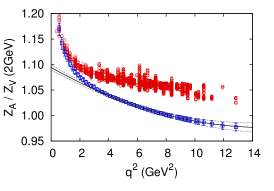
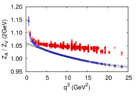
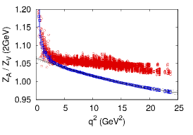
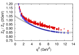
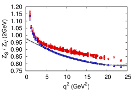
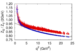
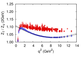
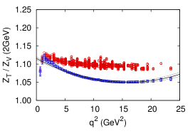
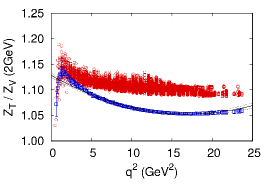
Figure 11: Ratios of renormalization constants $Z_{A}/Z_{V}$, $Z_{S}/Z_{V}$ and $Z_{T}/Z_{V}$ in the $\overline{\text{MS}}$ scheme at $2\mathop{\rm GeV}\nolimits$ using method C. The rest is the same as in Fig. 10.

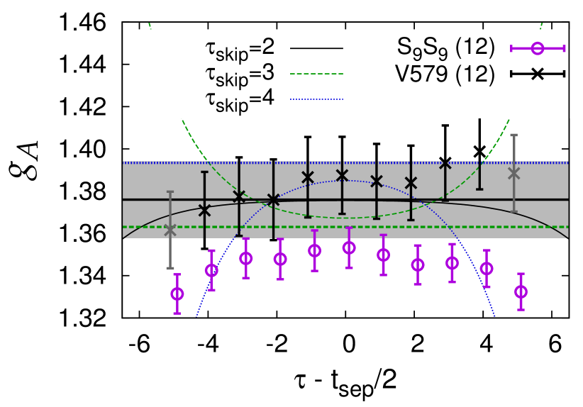
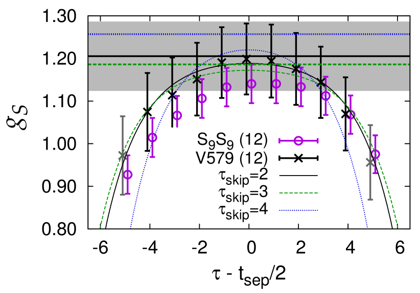
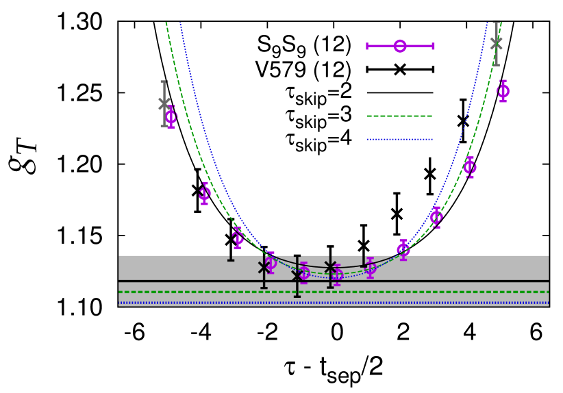
Figure 12: The projected variational three-point correlation function (black crosses) for the three isovector charges obtained from simulations with $\mathop{t_{\rm sep}}\nolimits=12$ on the $a094m280$ ensemble. The raw data is the same as that presented in Ref. Yoon et al. (2016) and labeled V579. The new fits with the full covariance matrix are shown for three values of $\mathop{\tau_{\rm skip}}\nolimits=2,3,4$. The variational result (solid black line) and the grey error band is the result of the fit with $\mathop{\tau_{\rm skip}}\nolimits=2$. For comparison, we also show the data points for the $S_{9}S_{9}$ correlation function (purple circles) with $\mathop{t_{\rm sep}}\nolimits=12$.

The second comparison we make is with results given in Ref. Yoon et al. (2016) obtained using the variational method on the $a094m280$ ensemble. The results from the variational analysis of the $3\times 3$ matrix of two- and three-point correlations functions constructed using the smearing parameter values $\sigma=5,7$ $9$ at a single value of $\mathop{t_{\rm sep}}\nolimits=12$ are also given in Tables 13 and  14. These numbers, labeled VAR579, are different from those presented in Ref. Yoon et al. (2016) as the fits have now been done using the full covariance matrix and the renormalization factors have been included. The results from the 2-state fits presented in this work and those from the variational method are in very good agreement.

In Fig. 12, we show the projected variational three-point correlation function for the three isovector charges on the $a094m280$ ensemble, taken from the data presented in Ref. Yoon et al. (2016). The curved lines show the 2-state fit to these data for three values of $\mathop{\tau_{\rm skip}}\nolimits=2,3,4$. The corresponding three $\mathop{t_{\rm sep}\to\infty}\nolimits$ estimates agree and lie within the shaded $1\sigma$ band for the $\mathop{\tau_{\rm skip}}\nolimits=2$ fit. The panels also show the $S_{9}S_{9}$ correlation function data with $\mathop{t_{\rm sep}}\nolimits=12$ (purple circles). Note that the variational analysis has been done on only 443 configurations versus the full set of 1005 for the $S_{9}S_{9}$ study. The errors in the two sets of data points are comparable once this difference in statistics is taken into account.

The data for $g_{A}^{u-d}$ in the top panel of Fig. 12 are almost flat in $\tau$ for both methods, suggesting that the contribution of the $\langle 0|\mathcal{O}_{A}|1\rangle$ term to both the variational and the tuned $S_{9}S_{9}$ correlation functions is small. The variational estimates lie about $3\%$ higher. A difference of this size can easily be explained by possible differences in the $\langle 1|\mathcal{O}_{A}|1\rangle$ or higher terms that cannot be isolated from fits to data with a single value of $\mathop{t_{\rm sep}}\nolimits$.

The data for the scalar channel exhibits significant curvature in both correlation functions and this $\tau$-dependence is again almost entirely accounted for by the $\langle 0|\mathcal{O}_{S}|1\rangle$ term. The $\approx 1\sigma$ difference between the two correlation functions is most likely again due to differences in the contributions of the $\langle 1|\mathcal{O}_{S}|1\rangle$ and higher terms. In the tensor channel, the data show very little change with the smearing parameter $\sigma$, and the variational and the $S_{9}S_{9}$ estimates essentially overlap.

This comparison indicates that the most significant gain on using the variational method with $\mathop{t_{\rm sep}}\nolimits=12$ is in $g_{A}^{u-d}$. Further calculations are needed to understand why the excited-state behavior is so different in the three charges. Based on the current data, to confirm that estimates in the $\mathop{t_{\rm sep}\to\infty}\nolimits$ limit have been obtained, the variational analysis needs to be repeated at values of $\mathop{t_{\rm sep}}\nolimits>12$ and the 2-state fit with multiple values of $\mathop{t_{\rm sep}}\nolimits$ requires high-precision data at $\mathop{t_{\rm sep}}\nolimits>1.2$ fm.

VII Conclusions

We have presented a high statistics study of isovector charges of the nucleon using four ensembles of (2+1)-flavor clover lattices generated using the RHMC algorithm Duane et al. (1987). The all-mode-averaging method Bali et al. (2010); Blum et al. (2013) and the coherent source sequential propagator technique Bratt et al. (2010); Yoon et al. (2016) are shown to be cost-effective ways to increase the statistics. We demonstrate control over excited-state contamination by performing simulations at multiple values of the source-sink separation $\mathop{t_{\rm sep}}\nolimits$, and by showing the stability of the 2-, 3- and 4-state fits.

The first highlight of the analysis is that $O(10^{5})$ measurements allowed us to carry out 2-, 3- and 4-state fits to the two-point functions and 2- and 3-state fits to the three-point correlation functions using the full covariance matrix. In all cases, except for the $a091m170L$ ensemble that is statistics limited, the results for the nucleon mass, the mass-gaps and the charges show stability with respect to variations in the fit parameters and the number of states included in the fits. Based on this analysis, we estimate that it will take $O(10^{6})$ measurements to obtain results for $g_{A,T,V}$ with $O(1\%)$ ($g_{S}$ with $O(3\%)$) error on each ensemble.

The second highlight is that our clover-on-clover results are in good agreement with calculations done using the clover-on-HISQ lattice formulation with similar values of the lattice parameters Bhattacharya et al. (2015, 2016); Gupta et al. (2015). Estimates of $g_{A}$, considered a litmus test of lattice QCD’s promise to provide precise estimates of the nucleon structure, are within $5\%$ of the experimental value even with light quark masses corresponding to $M_{\pi}\approx 280$ and $170$ MeV. These calculations are being extending to lighter quarks to study the chiral behavior and to finer lattice spacings to carry out the continuum extrapolation.