Electron transport parameters in CO2: scanning drift tube measurements and kinetic computations
Abstract
This work presents transport coefficients of electrons (bulk drift velocity, longitudinal diffusion coefficient, and effective ionization frequency) in CO2 measured under time-of-flight conditions over a wide range of the reduced electric field, in a scanning drift tube apparatus. The data obtained in the experiments are also applied to determine the effective steady-state Townsend ionization coefficient. These parameters are compared to the results of previous experimental studies, as well as to results of various kinetic computations: solutions of the electron Boltzmann equation under different approximations (multiterm and density gradient expansions) and Monte Carlo simulations. The experimental data extend the range of compared with previous measurements and are consistent with most of the transport parameters obtained in these earlier studies. The computational results point out the range of applicability of the respective approaches to determine the different measured transport properties of electrons in CO2. They demonstrate as well the need for further improvement of the electron collision cross section data for CO2 taking into account the present experimental data.
pacs:
52.25.Fi1 Introduction
The current (2016) atmospheric CO2 concentration is 404.21 ppm and it undergoes a constant growth [1]. In order to avoid its serious consequences foreseen at higher concentrations, the CO2 production must be reduced. One possible solution is the utilization of CO2, that is, the conversion of CO2 into more valuable chemical compounds that can be used as fuel or feedstock gas for different chemical processes (e.g. methanol or CO [2, 3, 4]).
The amount of energy necessary for this conversion could be gained from renewable energy sources (e.g. wind and solar cells) during the periods when the production of electricity exceeds the demands. As mentioned above, CO2 can be split to CO an O2 via the reaction . Plasma technologies have been gaining increasing interest for CO2 conversion [5, 6]. The energy efficiency and the conversion rate have been examined in dielectric barrier discharges [7, 4, 8, 9, 10, 11], corona discharges [12, 13, 14], gliding arc discharges [15], radio-frequency discharges [16], and nanosecond repetitively pulsed discharges [17].
In order to promote the plasma-based chemical technologies, it is crucial to improve knowledge about the fundamental properties of the interactions taking place in the plasma phase, which are characterized by the collision cross sections or rates of relevant plasma-chemical processes and transport parameters of relevant particles. Among all the particles, electrons play a central role. Therefore, their transport coefficients are of fundamental interest.
Drift tubes have been serving as the principal sources of transport coefficient data throughout several decades. In these systems low density clouds or “swarms” of electrons are created, which propagate under the influence of an external electric field. Based on their operation principles drift tube experiments have three major types [18]:
-
•
Pulsed Townsend (PT) settings consist of two plane-parallel electrodes. Electron swarms are usually initiated by fast UV light pulses that induce photoemission of electrons from the negatively biased electrode. Recordings are made of the time-dependent displacement current pulses.
-
•
Time-of-flight (TOF) settings employ as well pulsed electron sources and make use of the collection of particles that arrive at a detector, which can operate on the basis of different principles. In this case, the same transport coefficients can usually be determined as in PT settings.
-
•
Steady-state Townsend (SST) settings operate with continuous electron sources and provide information about the Townsend ionization coefficient, via, e.g. the increase of the electron current with increasing electrode separation.
In pulsed systems in the hydrodynamic regime with the electric field in the direction, the theoretical spatio-temporal distribution of the electron density of a swarm generated at time and position can immediately be derived from the solution of the continuity equation. It is given by [19]
| (1) |
where is the initial electron density, is the longitudinal diffusion coefficient, is the effective ionization frequency (equal to ionization frequency minus attachment frequency), and is the bulk drift velocity, which gives the velocity of the center-of-mass of the electron cloud.
In PT experiments the measured displacement current is proportional to the spatial integral of under hydrodynamic conditions. In contrast, in TOF systems (including our experimental system) the measured signal is directly proportional to (under hydrodynamic conditions), and the extraction of the transport coefficients proceeds via fitting the measured signals with the theoretical form (1). This procedure yields the bulk drift velocity , the longitudinal diffusion coefficient , and effective ionization frequency .
Our experimental apparatus allows “mapping” of the electron swarms [20, 21] by taking measurements at a large number of drift lengths. The swarm maps generated this way allow a visual observation of the equilibration of the transport as well, and a straightforward distinction between hydrodynamic and non-hydrodynamic domains can be done. Besides the “basic” TOF transport coefficients (, , and ), the application of the well-known connection between TOF and SST transport coefficients also allows us to derive the effective (steady-state) Townsend ionization coefficient [22, 19].
In the present paper we revisit the electron transport coefficients in carbon dioxide in the range of reduced electric fields between 15 and 2660 Td, where . Our measured data are compared with experimental results of earlier studies compiled in the review of Dutton [23] as well as of more recent analyses reported in [24, 25, 26, 27, 28]. Corresponding theoretical studies of electron transport properties in CO2 have been presented e.g. in [29, 30, 31, 32, 33, 34]. These results were obtained by Boltzmann equation and/or Monte Carlo simulation methods, where different data for the electron collision cross sections were used.
In addition to the experimental investigations we also carry out computations of the transport coefficients using different types of theoretical methods. Besides Monte Carlo simulations, the electron Boltzmann equation is solved under different assumptions and approximations. The application of these different approaches allows us to mutually verify the accuracy of the different methods, test the assumptions used by each method and uncover errors in the codes [35]. Furthermore, information about the respective transport properties provided by each method is given. The numerical calculations and simulations are performed using the recently published set of electron collision cross sections reported in [36].
The manuscript is organized as follows. In section 2 we give a concise description of our experimental setup and introduce the methods of data evaluation. A discussion of the various computational methods and the resulting transport properties is presented in section 3. It is followed by the discussion of the results in section 4. This section comprises the presentation of the present experimental results and their comparison with previously available measured data in section 4.1 as well as the comparison between transport parameters computed using the various numerical methods and the present experimental data in section 4.2. Section 5 gives our concluding remarks.
2 Experimental apparatus and data acquisition
2.1 Experimental setup
The experiments are based on a “scanning” drift tube apparatus of which the details have been presented in [20] and which has already been applied for the measurements of transport coefficients of electrons in various gases: argon, synthetic air, methane, and deuterium [21]. Our system – in contrast with previously developed drift tubes – allows recording of “swarm maps” that show the spatio-temporal development of electron clouds under TOF conditions. The simplified scheme of our experimental apparatus is shown in figure 1 and its brief description is given below.
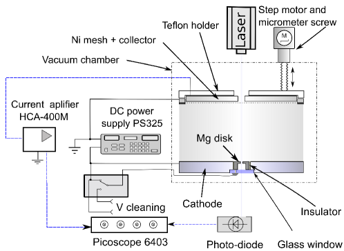
Electron swarms are initiated at 3 kHz repetition rate by , pulses of a frequency-quadrupled diode-pumped YAG laser that irradiates a magnesium disk embedded inside a stainless steel cathode electrode having a diameter of 105 mm (see figure 1). The swarms move under the influence of an electric field applied between the cathode and a grounded nickel grid (with 88 % transmission and 45 lines/inch density) situated at 1 mm (fixed) distance in front of a stainless steel collector electrode. The grid and the collector are moved together by a step motor connected to a micrometer screw mounted via a vacuum feedthrough to the vacuum chamber that encloses the drift cell. The distance between the cathode and the collector is scanned in 1 mm steps over the range of . The electric field is kept constant during the scanning process by automatically adjusting the cathode–collector voltage by a PS-325 (Stanford Research Systems) power supply. The laser pulses are also used for triggering the data collection. The current generated by the electrons entering the grid-collector gap is amplified by a high speed current amplifier (type Femto HCA-400M) and is acquired by a digital oscilloscope (type Picoscope 6403B) with sub-ns time resolution. The measured current signal is proportional to the flux of the electrons entering the grid-collector gap. As the flux and the density of the electrons are proportional in the hydrodynamic regime, the data shown in the form of “swarm maps” may also be interpreted as the electron density. We note that the non-hydrodynamic behavior can directly be identified in the swarm maps as it was demonstrated earlier [20]. This (i) allows us to restrict our data evaluation procedures to the domain where hydrodynamic equilibrium prevails, and (ii) makes it unnecessary to find this domain by numerical simulations of the experimental system.
Preceding the experiments the vacuum chamber is evacuated by a turbomolecular pump backed by a rotary pump down to a base pressure of for several days. During the experiments a slow (5 sccm) flow of (5.0 purity) CO2 gas is established by a flow controller, and the gas pressure inside the chamber is measured by a Pfeiffer CMR 362 capacitive gauge. The experiment is fully controlled by a LabView program. The measurements are performed at room temperature of 293 K. In order to prevent the electrical breakdown of the gas the experiments had to be conducted at different pressures, i.e., at different values of , for different domains of the whole range. Of course, this was done with an overlap of the values when changing the pressure, to allow observation of an eventual dependence of the experimental data on the change of pressure. As we used the hydrodynamic regime for the evaluation of the swarm characteristics such dependence was actually not observed.
2.2 Data acquisition
As it was already mentioned in section 1, the transport coefficients , , and are derived by fitting the experimentally measured signal of the current to the theoretical form (1) of the electron density describing the spatio-temporal evolution of the swarm. It is important that this fitting is executed for hydrodynamic conditions. Deviations from the hydrodynamic condition are easy to recognize in the measured swarm maps, however [20]. In cases when such deviations are observed, the fitting is executed for a part of the space-time domain where equilibrium transport prevails. In this fitting procedure we select the complete map, as well as its sub-domains, and accept the resulting values of the transport coefficients only when the fits over different domains give data within a pre-defined deviation from each other (see below).
The uncertainties of the determination of the transport coefficients mainly originate from the errors and fluctuations of the experimental characteristics: errors of the setting of the electrode gap, the pressure, the voltage across the cell, the (fluctuating) laser intensity, and electric noise. The fitting procedure was found not to enhance the uncertainties and fluctuations in the determination of , as in this case the position of the current peak is the most important quantity that is well defined even in the presence of noises. This is why we estimate the total accuracy of the determination of to be of the order of 3% based on our estimations of the errors in the measurements of the voltage, pressure, etc. The uncertainty of caused by the fitting procedure itself (selection of the fitting domain) proved to be less than 1%. On the other hand, the values of the resulting were sensitive on the choice of the domain of fitting. Here, we accept values that are within 15%, which seems to be a proper value considering the fact that previous studies have also reported values with such an accuracy. The larger sensitivity of the measured on the choice of the fitting domain originates from the fact that the determination of the width of the pulse is more sensitive on the signal to noise ratio, compared to the determination of the peak position.
Besides the fitting of the theoretical and measured density distributions, we also apply a slicing method for the determination of the bulk drift velocity for values below 1000 Td: cutting the maps of the swarm (or the density distribution (1)) at fixed values of time, symmetrical Gaussian functions are obtained and the peaks of these functions can be associated with the center-of-mass of the swarm. A straight line fit to this position as a function of time yields the value of [20]. The results obtained for by both the fitting procedure and the slicing method agree more closely than 1 %.
Having determined the TOF transport coefficients , , and , the effective Townsend ionization coefficient, , characteristic of SST experiments, is calculated according to
| (2) |
based on the discussions in the papers of Tagashira et al. [22] and of Blevin and Fletcher [19]. In the absence of diffusion, i.e., , eq. (2) reduces to . This value is increased in the presence of diffusion and, for the gases and conditions covered here, this increase is between 1 % and 20 %.
3 Numerical methods
The experimental studies of the electron transport parameters are supplemented by results obtained by numerical modeling and simulation. In addition to Monte Carlo (MC) simulations, three different methods are applied to solve the Boltzmann equation (BE) for electron swarms in a background gas with density and acted upon by a constant electric field, , and assuming hydrodynamic conditions: (i) a multiterm method for the solution of the time- and space-independent Boltzmann equation , (ii) a multiterm approach for solving the spatially one-dimensional, steady-state electron Boltzmann equation as well as (iii) the method applied to a density gradient expansion of the electron distribution function. They differ in their initial physical assumptions and in the numerical algorithms used and provide different properties of the electrons. In the following, a brief description of these three methods as well as main aspects of the MC simulation approach are given. In this discussion, the electric field is along the axis pointing in negative direction, , and is the angle between and . Moreover, we assume that after a sufficiently long relaxation time and length the transport properties of the electrons do not change with time and distance any longer, i.e., the electrons have reached a hydrodynamic regime characterizing a state of equilibrium of the system where the effects of collisions and forces are dominant and the electron velocity distribution function has lost any memory of the initial state.
For our studies we use the electron–CO2 collision cross section set recently published in [36], however, we neglect superelastic collision processes. The data set used includes the momentum transfer cross section for elastic collisions, 11 vibrational and two electronic excitation cross sections, the total electron-impact ionization cross section and the collision cross section for dissociative electron attachment to CO2. The cross section data are illustrated in figure 2.

3.1 Multiterm method for spatially homogeneous conditions
To study the electron movement under the conditions mentioned above, we need further assumptions on the system and the electron velocity distribution function. In our first Boltzmann equation approach (abbreviated by BE 0D in the figures shown in section 4) we consider a spatially homogeneous system where the electron density changes exponentially in time according to , depending on the effective ionization frequency . In this case we can neglect the dependence of on the space coordinates and write the velocity distribution function under hydrodynamic conditions as
| (3) |
The corresponding microscopic and macroscopic properties of the electrons are determined by the time-independent, spatially homogeneous Boltzmann equation for . This distribution is symmetric around the field direction, , where is the component of the velocity with magnitude . Thus, an expansion of the velocity distribution function with respect to in Legendre polynomials according to
| (4) |
becomes possible, where the magnitude of the velocity was replaced by the kinetic energy of the electrons with mass on the right-hand side. Substitution of expansion (4) including an arbitrary number of expansion coefficients into the electron Boltzmann equation finally leads to a hierarchy of partial differential equations for the expansion coefficients with . The normalization condition is . The resulting set of equations with typically eight expansion coefficients is solved employing a generalized version of the multiterm solution technique for weakly ionized steady-state plasmas [37] adapted to take into account ionizing and attaching electron collision processes. The need for such multiterm approximation for the analysis of steady-state plasmas was found to arise in general when the lumped collision cross section of all inelastic collision processes is large and becomes comparable with the total cross section for elastic collisions over large parts of the relevant energy regions[32, 38]. Under such conditions, the coupling in the hierarchy of expansion coefficients leads to a large anisotropy of the electron velocity distribution function.
The macroscopic properties for spatially homogeneous conditions, namely the flux drift velocity
| (5) |
where is the mobility, the flux diffusion coefficients and , the ionization and attachment frequencies and , can be obtained using the equations given in [39, 40]
| (6) | |||||
| (7) | |||||
| (8) | |||||
| (9) |
Here, is the elementary charge,
| (10) |
with being the sum of the elastic momentum transfer cross section and all inelastic cross sections, and denote the ionization and attachment cross sections, and . Furthermore, the effective ionization coefficient for spatially homogeneous plasmas is given by
| (11) |
3.2 Multiterm method for spatially inhomogeneous conditions
In the second Boltzmann equation approach (designated as BE 1D SST below) we consider the spatial relaxation of an electron swarm. In this case we determine the effective Townsend ionization coefficient, , characteristic of SST experiments. Here, an idealized SST experiment with plane-parallel geometry similar to [41, 42] is considered, where a steady flux of electrons is emitted from the cathode. These electrons are accelerated in the positive direction under the action of the electric field, ionize the gas or are attached by it. At a sufficiently large distance from the cathode, the mean transport properties of the electrons do not vary with position any longer and the electron density assumes the exponential dependence on the distance
| (12) |
where is a constant.
In order to determine the microscopic and macroscopic properties of the electrons under such conditions, the spatially one-dimensional Boltzmann equation for their velocity distribution function is solved. As the electric field and the inhomogeneity in the plasma are both parallel to the axis, this distribution function is also symmetric around the field direction, i.e., . Thus, we can expand the velocity distribution function in Legendre polynomials in accordance with (4), where the expansion coefficients are functions of and now and the normalization on the electron density according to
| (13) |
holds. Substitution of this expansion into the Boltzmann equation of the electrons results in a set of partial differential equations for the expansion coefficients with in the end. This equation system is solved numerically in accordance with the multiterm solution method described in [43] using typically expansion coefficients.
The consistent particle balance of the electrons reads
| (14) |
where appropriate energy space averaging over the normalized expansion coefficients with and 1 yields the space-dependent mean electron velocity in direction as well as the space-dependent frequencies of ionization and of attachment , respectively. The latter are determined according to (9). The mean velocity given as [40]
| (15) |
is composed of the space-dependent flux drift velocity , which is in accordance with (5), and a diffusion part. It can be written as
| (16) |
where the space-dependent electron mobility and the flux longitudinal diffusion coefficient as well as the flux transverse diffusion coefficient are given by similar integration over as (6), (7) and (8) with replaced by [40, 39].
When approaching SST conditions at a sufficiently large distance from the cathode, the normalized expansion coefficients and, consequently, the macroscopic properties , , , , and become independent of the position . Then, the particle balance equation (14) becomes
| (17) |
where the upper index denotes the SST condition. Using equations (12) and (17), thus the effective Townsend ionization coefficient is directly given by
| (18) |
or dependent on the non-observable quantities , , and [19] according to
| (19) |
Notice that although relation (18) has the same form as the effective ionization coefficient (11) for spatially homogeneous conditions, both parameters are generally not identical. Furthermore, the effective (steady-state) Townsend ionization coefficient calculated from the TOF transport coefficients according to (2) looks similarly but gives a different result from relation (19). However, the values of obtained from (2) and (19) are identical, if higher-order terms in the derivation of (2) are neglected, as usually assumed in the TOF case [22, 19].
Following Blevin and Fletcher [19], the SST parameters can be expressed by a series expansion with respect to . The application of such expansion and its correlation with the density gradient expansion discussed in section 3.3 make it possible to approximately determine the bulk drift velocity from the SST calculations. Then, we can get from the approximation equation
| (20) |
provided that the flux drift velocity according to (5) and the effective ionization frequency for spatially homogeneous conditions are known in addition to the mean velocity and the effective Townsend ionization coefficient at SST conditions.
Finally, it should be mentioned that the application of (12) and the assumption of SST conditions also leads to a set of equations for . This equation system can also be solved efficiently by a modified version of the multiterm technique method [37] adapted to treat SST conditions. Corresponding results show excellent agreement with the SST results obtained by using the method BE 1D SST and are therefore not included in the figures presenting our results, in favour of clarity.
3.3 Density gradient representation
The third Boltzmann equation approach to describe the electron swarm at hydrodynamic conditions (labelled as BE DG TOF below) is based on an expansion of the electron velocity distribution function, , on the consecutive space gradients of the electron density . In this case, depends on only through the density and can be written as an expansion on the gradient operator according to
| (21) |
Here, the expansion coefficients are tensors of order depending only on , and indicates a -fold scalar product [44]. Note that the first coefficient corresponds to the conventional distribution function for homogeneous conditions, denoted by in equation (3) in section 3.1.
Each expansion coefficients of order is obtained from a hierarchy of equations for each component depending on the previous orders and all with the same structure. In particular, a total of five equations is required, namely for the coefficients components , , , and . In the present code these equations are solved using a variant of the finite element method given in [45] in a grid.
The transport parameters for a TOF experiment are obtained from the above expansion coefficients as
| (22) | |||||
| (23) | |||||
| (24) | |||||
| (25) |
where , , , and are the bulk drift velocity, the bulk diagonal longitudinal and transverse components of the diffusion tensor, and the effective ionization frequency, respectively, and . Here, the lower indexes and on the right indicate the longitudinal and transverse components of the vectors and and the diagonal terms of the tensor . The corresponding flux components of the drift velocity and the diffusion tensor are the first terms on the right-hand side of equations (22)–(24). The second term on the right-hand side of these equations describes the explicit contribution of the non-conservative collision processes by the velocity-space averaging over the product of and the expansion coefficients of order 1 and 2, respectively.
The effective or apparent Townsend ionization coefficient , as determined in SST experiments, can be computed either from , the distribution function at SST conditions obtained from the solution of an additional equation similar to the one for the expansion coefficient , as [46]
| (26) |
or from the TOF parameters using the relation [22, 19]
| (27) |
which is the inverse representation of equation (2).
It can be shown that the flux component () of (22) has the same expression as (15) and that equation (25) divided by is equivalent to as given by (9). In the case of the diffusion tensor, the comparison is more complex. Using the Boltzmann equation for each component of , we can rewrite equations (23) and (24) as [46, 35]
| (28) | |||||
| (29) | |||||
where is the acceleration due to the electric field and . However, only the terms involving are comparable with equations (7) and (8). The second terms represent contributions from the electric field and the gradient of the distribution of electrons with different velocities inside the swarm, as given by , to the spreading of the swarm. The third terms are the contribution of non-conservative processes. Using the index ”” to designate the first term of (28) and (29), after an expansion in Legendre polynomials and a change of variables from to , these terms can be written as
| (30) | |||||
| (31) |
Except for the last term in (30), these are the same expressions as (7) and (8). Notice that a similar representation was derived in [39] for the case of conservative electron collision processes.
3.4 Monte Carlo method
In the MC simulation technique we trace the trajectories of the electrons in the external electric field and under the influence of collisions. Due to the low degree of ionization under the swarm conditions considered here, only electron-background gas molecule collisions are taken into account. The motion of the electrons between collisions is described by their equation of motion
| (32) |
The determination of the electron trajectories between collisions is carried out by integrating (32) numerically over time steps of duration ranging between 0.5 and for the various conditions. While this procedure is totally deterministic, the collisions are handled in a stochastic manner. The probability of the occurrence of a collision is computed after each time step, for each of the electrons, as
| (33) |
Comparison of with a random number having a uniform distribution over the interval allows deciding about the occurrence of a collision: if a collision is simulated. This is carried out in the center-of-mass frame (for a more detailed description see, e.g., [47]). The type of collision is also determined in a random manner; the probability of process at a given energy is given by
| (34) |
where is the collision cross section of the -th process. The elastic collisions are assumed to result in isotropic scattering. Accordingly, we use the elastic momentum transfer cross section.
We carry out two types of MC simulations:
-
•
TOF simulations (labeled as MC TOF below) are executed to determine the bulk () and flux () drift velocities of the electrons according to
(35) and
(36) Here, is the number of electrons in the swarm at time . Note that when expanding (35), we obtain the relation between these velocities as , where is the average position and
(37) showing how includes a contribution from non-conservative processes. These simulations also yield the longitudinal and transversal diffusion coefficients and obtained as [48]
(38) (39) Furthermore, the effective Townsend ionization coefficient can be calculated according to relation (2) using (35), (37), and (38) and neglecting higher-order terms in the derivation of (2) as usually done in the TOF case [22, 19].
-
•
SST simulations (named as MC SST below) are additionally used to derive directly the effective Townsend ionization coefficient from the spatial growth of the electron density under stationary conditions according to
(40)
3.5 Summary of computational methods
The computational methods used to derive the transport coefficients of electrons for different conditions, as well as the resulting transport coefficients are summarized in Table 1.
| Id. | Method | Transport coefficients | ||
|---|---|---|---|---|
| bulk | flux | change | ||
| BE 0D | Spatially homogeneous BE | , , | , | |
| BE 1D SST | 1-dimensional stationary BE | , , | , | |
| BE DG TOF | Density gradient expansion of BE | , , | , | |
| BE DG SST | Density gradient expansion of BE | |||
| MC TOF | Time-of-flight MC simulation | , , | , | |
| MC SST | Stationary MC simulation | |||
4 Results
Measurements of the electron transport coefficients have been performed in the wide range of the reduced electric field between 15 and 2660 Td at a gas temperature of 293 K. The results of our measurements are presented and discussed in the following. In section 4.1, they are compared with previous experimental data. Section 4.2 adds a comprehensive comparison with results obtained by the different Boltzmann equation methods and by MC simulations.
4.1 Experimental data and comparison with previous experimental results
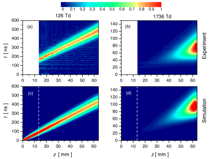
We begin the presentation of the results by illustrating the measured swarm maps in comparison with simulated maps obtained by the MC TOF method. Figure 3 shows the maps for two different sets of experimental conditions with and as well as and at room temperature, corresponding to the values of the reduced electric field and 1736 Td, respectively. The maps allow a straightforward visual observation of the characteristic effects of drift, diffusion and ionization. In this representation of the spatio-temporal distribution of the electron density the inclination of the path of the electron cloud corresponds to its drift. The widening of the cloud is related to the effect of diffusion, while the increase of density with the spatial coordinate and with time is a signature of avalanching through ionization processes at these ionization-dominated conditions. Notice that for attachment-dominated conditions with between about 30 and 90 Td [25] a decrease of the density should equally be observable. At the low reduced electric field of (figures 3(a) and (c)) the electron cloud exhibits a small spreading and small density increase, indicating low rate of diffusion and low effective ionization. This behavior changes remarkably when is increased. At 1736 Td the increasing importance of both diffusion and ionization processes changes the character of the swarm map noticeably as illustrated in figures 3(b) and (d). These features are well represented by both the experimental and simulated results.
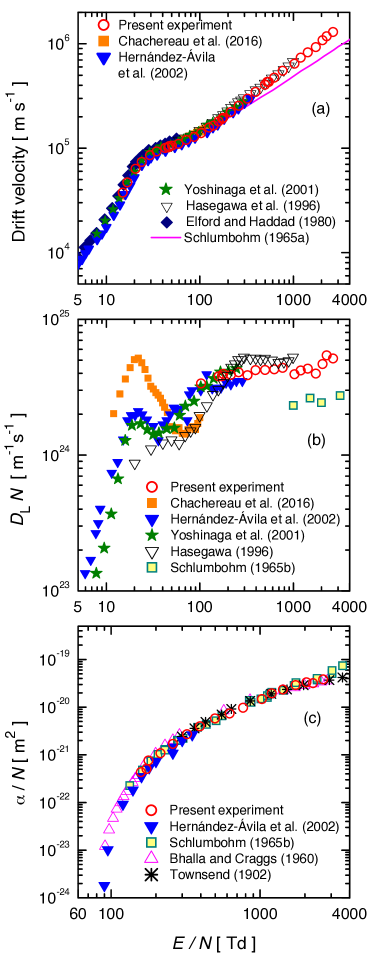
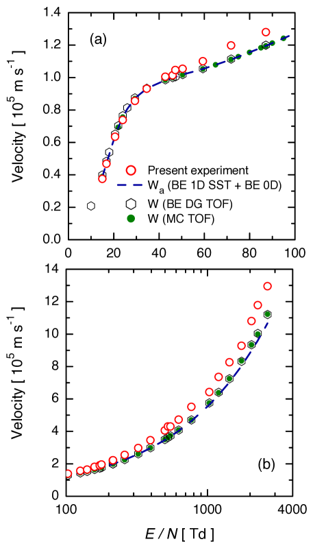
Our experimental results for the transport coefficients are displayed in figure 4. The panels (a), (b), and (c) show the measured bulk drift velocity , the measured longitudinal diffusion coefficient times gas number density and the reduced effective Townsend ionization coefficient , respectively. The latter is calculated according to (2) using the measured effective ionization frequency in addition to and . Tabulated values of the transport coefficients as a function of the reduced electric field are also given in tables 2 and 3. Table 2 contains the measured values of the bulk drift velocity at between 15 and 2660 Td. Table 3 gives the longitudinal diffusion coefficient, effective ionization frequency, and the effective Townsend ionization coefficient in the range of the reduced electric field from 159 to 2660 Td.
| 15.0 | 3.75 | 50.4 | 10.5 | 173 | 19.0 | 625 | 47.3 |
| 16.8 | 4.68 | 59.4 | 11.0 | 178 | 19.6 | 769 | 55.1 |
| 20.6 | 6.35 | 71.8 | 12.0 | 214 | 22.1 | 1030 | 64.3 |
| 24.0 | 7.39 | 87.1 | 12.9 | 260 | 25.5 | 1200 | 73.6 |
| 29.4 | 8.56 | 87.2 | 12.8 | 324 | 29.7 | 1430 | 82.6 |
| 34.6 | 9.31 | 103 | 13.9 | 395 | 34.6 | 1740 | 92.8 |
| 42.8 | 10.1 | 126 | 15.7 | 499 | 40.5 | 2050 | 108 |
| 46.0 | 10.1 | 141 | 16.4 | 525 | 43.0 | 2270 | 118 |
| 47.2 | 10.5 | 159 | 18.1 | 547 | 43.0 | 2660 | 130 |
| 159 | 3.79 | 0.00777 | 0.0432 |
|---|---|---|---|
| 173 | 3.81 | 0.00950 | 0.0504 |
| 178 | 3.96 | 0.0147 | 0.0759 |
| 214 | 3.89 | 0.0235 | 0.108 |
| 260 | 4.07 | 0.0421 | 0.169 |
| 324 | 3.87 | 0.0772 | 0.270 |
| 395 | 4.22 | 0.129 | 0.395 |
| 499 | 4.23 | 0.218 | 0.578 |
| 625 | 4.28 | 0.316 | 0.732 |
| 769 | 4.39 | 0.475 | 0.968 |
| 1030 | 3.94 | 0.833 | 1.48 |
| 1200 | 4.19 | 1.27 | 1.95 |
| 1430 | 4.32 | 1.71 | 2.35 |
| 1740 | 3.98 | 2.31 | 2.89 |
| 2050 | 4.68 | 3.06 | 3.31 |
| 2270 | 5.42 | 3.28 | 3.19 |
| 2660 | 5.14 | 4.19 | 3.83 |
Our experimental results are compared with experimental data reported in [24, 25, 26, 27, 28, 49, 50, 51, 52]. Specific features of these experimental investigations are given in the following. Chachereau et al. [24] used a PT apparatus with a back-illuminated photocathode. The electron drift velocity and the longitudinal electron diffusion coefficient were determined by fitting the measured displacement current waveform with a theoretical form. Furthermore, the effective ionization rate coefficient was obtained using an electron swarm model. Results for CO2 were reported for reduced electric fields between 10 and 100 Td. Hernández-Ávila et al. [25] used as well a PT system equipped with a nitrogen laser to initiate photoelectron pulses. Displacement current pulses were measured at a fixed gap length of 30 mm at values ranging from 2 to 350 Td. These studies provided results for , , and the effective ionization coefficient , which is identical to according to (2) only in the absence of diffusion [23]. Yoshinaga et al. [26] employed a double-shutter drift tube with variable gap length between 10 and 50 mm. Photoelectrons were initiated by pulsed UV light from a quartz window covered with a gold film. The bulk drift velocity and longitudinal diffusion coefficient were measured over the range from 8 to 300 Td in this experiment. Hasegawa et al. [27] determined the electron drift velocity as well as the ratio of the longitudinal diffusion coefficient to the electron mobility (longitudinal characteristic energy) from the arrival time spectra of electrons in a double-shutter drift tube. Using both these measured quantities, we computed the values shown in figure 4(b). Their experiment covered the range of . Elford and Haddad [28] used the Bradbury-Nielsen type TOF method to measure the drift velocity of electrons at different temperatures. Their measurements extended over values between 0.1 and 50 Td at . Schlumbohm used a PT apparatus, operated with photoelectrons initiated by short () UV light pulses and described in [53], to measure the drift velocity [49] for about . These results were given in functional form of depending on at 293 K and corresponding tabulated data can be found e.g. in [23]. In addition, measured results of the effective ionization coefficient for about and the ratio were reported in [50]. The latter was used to determine the longitudinal diffusion coefficient in the range from 1000 to 3162 Td [23]. The SST method was used in [51, 52] to determine the effective Townsend ionization coefficient . Bhalla and Craggs [51] carried out measurements for the range from about 90 to 2825 Td and Townsend’s data [52] cover the range between about 300 and 3600 Td. Corresponding tabulated data can be found e.g. in [23]. Our drift velocity data (figure 4(a)) agree well with most of those given in these previous works, which also show a good degree of consistency. The only exception concerns the experimental data of Schlumbohm [49] at larger than 450 Td, where increasing differences are obvious. The agreement between our data and the data given by Hasegawa et al. [27] is particularly good and our measurements extend the range of from 1000 Td in [27] to 2660 Td. We estimate the experimental error of the present bulk drift velocity data to be less than 3 % below 1000 Td and less than 5 % above this value.
The values of the longitudinal diffusion coefficient times gas number density shown in figure 4(b) exhibit larger scattering, which is explained by the higher uncertainty of the determination of in the experiments ( including our present data) as compared to that of the drift velocity. Our data for cover the range . Up to , our data agree reasonably with those of Hasegawa et al. [27] considering the uncertainties of both data sets quoted above. The values derived by Schlumbohm [50] for are about a factor of two lower compared to the present data.
Figure 4(c) shows our experimental results for the effective Townsend ionization coefficient in comparison with the corresponding data provided by Bhalla and Craggs [51] and by Townsend [52] as well as the results for the effective ionization coefficient of Hernández-Ávila et al. [25] and Schlumbohm [50]. The different data sets show generally very good agreement. Our data cover the range of , for which the estimated experimental error of the data is approximately . For the accuracy of the determination of decreased drastically in our experiments due to the worse signal to noise ratio so that no data is available here.
4.2 Numerical results for transport coefficients and comparison with experimental data
In this section we present the results obtained by the various numerical methods described in section 3 using the cross section set from [36]. We compare the results with each other as well as with the present experimental data. A summary of the methods used to derive the transport coefficients of electrons for different conditions, as well as the resulting transport coefficients were given in table 1.
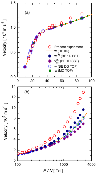
Figure 5 displays the flux drift velocity obtained by the different methods as well as the mean velocity at SST conditions derived according to (15). The latter is also referred to as diffusion-modified drift velocity in [22]. Furthermore, the present experimental data for the bulk drift velocity are shown for comparison. At low reduced electric fields (figure 5(a)) all computational approaches give consistent results, indicating as well that the contribution of the electron attachment e.g. on is rather small. However, at high (figure 5(b)) the agreement is retained only for the methods BE 0D, BE DG TOF and MC TOF. Because electron impact ionization processes are increasingly involved at larger , is known to become less than the flux drift velocity [42]. At the same time the flux drift velocity at SST conditions assumes larger values than the flux drift velocity obtained for the hydrodynamic regime of the time-dependent electron swarm. This finding is in agreement e.g. with the studies for argon reported in [22, 19]. It is also an immediate consequence of the establishment of different expansion coefficients (method BE 0D) and (method BE 1D SST), and thus the electron velocity distribution functions, under hydrodynamic and SST conditions, respectively. As an example, the corresponding first three expansion coefficients () are shown in figure 6. Similar results were also discussed e.g. for synthetic air at larger values in [54]. Moreover, the flux drift velocities shown in figure 5 remain increasingly smaller than the measured bulk drift velocity at larger because of the additional impact of the effective ionization on the latter.
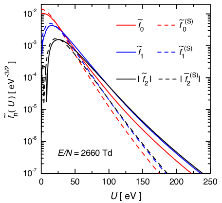
Figure 7 displays the bulk drift velocity computed by the MC TOF and DG TOF methods, an approximate value derived according to (20) from the combination of the calculated results of BE 1D SST and BE 0D and the present experimental results. The values from the MC TOF and DG TOF methods agree perfectly, while can be considered as a good approximation of up to about . The computed values are in good agreement with the experimental data at low fields of . Above this field strength the measured values are consistently higher than the computational results. The deviations between the experimental data and the TOF results amount between 10 and 15 % above 200 Td.
To interpret these results we must keep in mind that the cross section set used [36] was developed using a two-term expansion code, BOLSIG+ [55]. The transport parameters computed by this code can optionally include the effect of non-conservative processes and of the electron density gradients, depending on the problem being studied. In the derivation of the present cross section set the flux drift velocity [36, figure 3] was fitted at high to Schlumbohm’s results [49] for the bulk drift velocity . These results are lower than our and other experimental results at high , as can be seen in figure 4. Thus, the present computational results for the flux drift velocity in fact reproduce the experimental results of Schlumbohm and the apparent good fit of the computed values for the bulk drift velocity to the present experimental results in figure 7 is rather fortuitous.
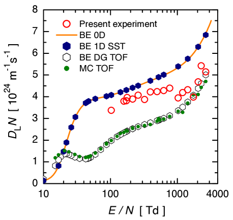
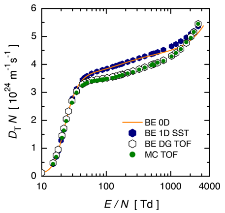
Computed values of the longitudinal () and transverse () diffusion coefficients are shown in figures 8 and 9, respectively. The values have been obtained by the BE 0D and BE 1D SST solutions as well as by the BE DG TOF and MC TOF methods. Available measured data for are also shown in figure 8 for comparison. The results of the methods BE 0D and BE 1D SST correspond to the respective flux components of the diffusion tensor and they practically overlap. The same is observed for the results obtained by the methods BE DG TOF and MC TOF, which correspond to the bulk components of the diffusion tensor. Regarding the longitudinal diffusion coefficient (figure 8), the BE DG TOF and MC TOF results can directly be compared with the experimental results for . None of the results, however, fits these experimental results for . In order to understand this finding, we note that in [36, figure 5] the high values for the flux component of are said to be fitted to the experimental results of Schlumbohm [50], which are below the present computed ones (cf. figure 4). Rather, it seems that the fit in [36, figure 5] was done using an expression equivalent to the first two terms of equation (28), i.e., including the effect of the electron density expansion but neglecting the contribution from non-conservative processes [56, page 16]. This was found to be comparable with our results obtained by the BE DG TOF and MC TOF methods, if we neglect the effect of non-conservative processes in the latter, i.e., assume and in (28).
The reduced ionization frequency computed by the different approaches as a function of the reduced electric field is displayed in figure 10. Good agreement between the measured and calculated results is generally found. This also holds for the reduced ionization frequency obtained by the BE 0D method, which perfectly agrees with the swarm-averaged computed by the methods BE DG TOF and MC TOF. Slight differences become visible at larger only for the reduced ionization frequency obtained for SST conditions using the method BE 1D SST. This finding indicates once more the differences between results obtained for SST conditions and for the hydrodynamic regime of time-dependent electron swarm studies. Similar differences were reported e.g. for argon in [22, 19].
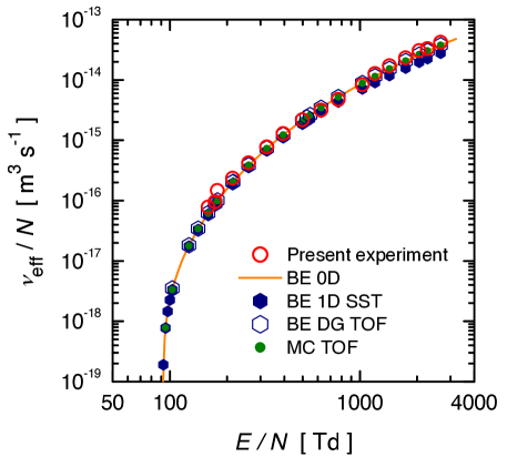
Figure 11 shows the effective Townsend ionization coefficient computed by the different SST and TOF methods (cf. table 1) and the present experimental obtained according to eq. (2) using the measured values of , and . Furthermore, the effective ionization coefficient determined by the method BE 0D is displayed. Figure 11(a) shows good agreement between all data sets in the double logarithmic representation. Certain differences between the results calculated by the different methods become obvious from the linear representation in figure 11(b), while the present experimental data still agree quite well with the computed .
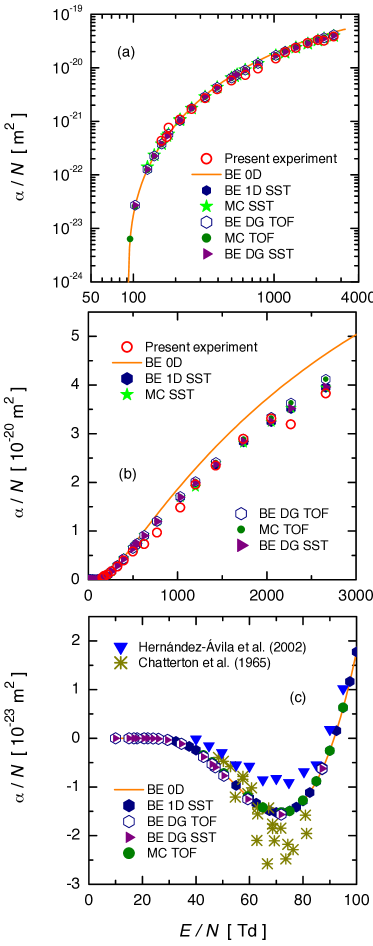
The consistent way to determine the effective Townsend ionization coefficient , relevant to SST conditions, is the use of the methods BE 1D SST, BE DG SST or MC SST. The corresponding data for are in excellent agreement in figure 11(b). Increasing differences from these results for are found for the effective ionization coefficient (11) obtained by the BE 0D method. These differences are natural, because and are different coefficients.
In addition, smaller, but increasing deviations between the results for obtained by the TOF methods BE DG TOF and MC TOF and those of the SST methods emerge above . Because both the BE DG TOF and MC TOF results agree excellently, it seems that the differences between the SST and TOF data result from the neglect of higher-order terms in the derivation of equations (2) and (27), respectively, used to determine in the TOF case [22, 19].
The low-field domain ( 100 Td) is analyzed in figure 11(c) in more detail. In this domain attachment dominates and ionization is hardly present. The computational results are consistent and show reasonable agreement with the two experimental data sets of Hernández-Ávila et al. [25] and Chatterton et al. [57], which are also shown in this figure.
5 Concluding remarks
We have investigated electron transport in CO2 gas experimentally using a scanning drift tube, as well as computationally by solutions of the electron Boltzmann equation and via Monte Carlo simulation, corresponding to both time-of-flight and steady-state Townsend conditions. The experimental system operated under TOF conditions and allowed recording the spatio-temporal evolution of electron swarms initiated by short UV laser pulses. The measured data made it possible to derive the bulk drift velocity, the longitudinal diffusion coefficient, and the effective ionization frequency of the electrons, for the wide range of the reduced electric field from 15 to . The measured TOF transport coefficients and the effective Townsend ionization coefficient, deduced from these coefficients, have been compared to experimental data obtained in previous studies, where generally good consistency with most of the transport parameters obtained in these earlier studies was found.
Comparison of the experimental data was also carried out with transport coefficients resulting from various kinetic computations, which used a cross section set published recently [36]. The computational results point out the range of applicability of the respective methods used to determine the different measured transport properties of electrons in CO2. In particular, significant differences between our measured and computed (by the TOF methods) values of the bulk drift velocity and the longitudinal diffusion coefficients have been found, which are attributable to the specific methods involved in the construction of the cross section set. Namely, this cross section set was developed neglecting the effect of non-conservative processes and fitting, at high , the results of Schlumbohm [49, 50] for and , which are significantly different from the present experimental results. Thus, the experimental results for the bulk drift velocity and longitudinal diffusion coefficients could not be reproduced correctly. However, the computational results obtained by all the methods used in this paper to determine the transport properties in the hydrodynamic regime show good agreement for the effective ionization frequency. Furthermore, the effective Townsend ionization coefficient calculated by the SST and TOF methods agree well with the results obtained from the experiments for the large range of investigated.
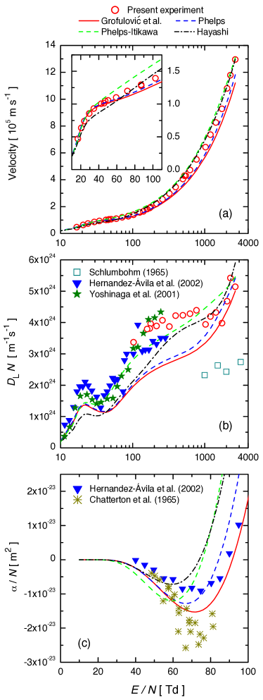
Other cross section sets, which are available for CO2 gas, do not perform better as well for all conditions and transport coefficients. A comparison of the computed bulk drift velocity, longitudinal diffusion coefficient and effective Townsend ionization coefficient using several different, widely used sets of cross sections is presented in figure 12. The cross section sets include the one by Grofulović et al. [36], that of Phelps [58], a modified cross section set of Phelps using the elastic momentum transfer cross section of Itikawa [59] (named Phelps-Itikawa set in the following), as well as the set recommended by Hayashi [60]. Figure 12(a) reveals that the drift velocity is best reproduced by the Phelps and the Grofulović et al. cross sections at low , while none of the computed values fits well our experimental data points for the range. A better agreement for the last few (high ) data points is found for the Phelps-Itikawa set and the Hayashi set. Computed values of (figure 12(b)) follow most closely the measured data up to moderate reduced electric field values () when the Phelps-Itikawa cross section set is used. At higher values the only experimental data in addition to Schlumbohm’s results [50] originate from the present measurements. Our data show a larger scattering, while the computed curves become closer and incidentally agree quite well with them. Regarding the effective ionization coefficient (figure 12(c)) no precise agreement is found for the low (attachment-dominated) domain with any of the computational results obtained with the different cross section sets.
Thus, we think that our present experimental results offer large potential for future adjustments of electron collision cross sections for CO2.
References
References
- [1] E. Dlugokencky and P. Tans. Recent Monthly Average Mauna Loa CO2, September 2016.
- [2] E. E. Barton, D. M. Rampulla, and A. B. Bocarsly. Selective solar-driven reduction of CO2 to methanol using a catalyzed p-GaP based photoelectrochemical cell. J. Am. Chem. Soc., 130(20):6342–6344, 2008.
- [3] Z. Zhan, W. Kobsiriphat, J. R. Wilson, M. Pillai, I. Kim, and S. A. Barnett. Syngas production by coelectrolysis of CO2/H2O: The basis for a renewable energy cycle. Energy Fuels, 23(6):3089–3096, 2009.
- [4] R. Aerts, W. Somers, and A. Bogaerts. Carbon Dioxide Splitting in a Dielectric Barrier Discharge Plasma: A Combined Experimental and Computational Study. ChemSusChem, 8(4):702–716, 2015.
- [5] A. Bogaerts, T. Kozak, K. van Laer, and R. Snoeckx. Plasma-based conversion of CO2: current status and future challenges. Faraday Discuss., 183:217–232, 2015.
- [6] A. Bogaerts, C. De Bie, R. Snoeckx, and T. Kozak. Plasma based CO2 and CH4 conversion: A modeling perspective. Plasma Process. Polym., in print.
- [7] D. Mei, X. Zhu, Y.-L. He, J. D. Yan, and X. Tu. Plasma-assisted conversion of CO2 in a dielectric barrier discharge reactor: understanding the effect of packing materials. Plasma Sources Sci. Technol., 24(1):015011, 2015.
- [8] F. Brehmer, S. Welzel, M. C. M. van de Sanden, and R. Engeln. CO and byproduct formation during CO2 reduction in dielectric barrier discharges. J. Appl. Phys., 116(12):123303, 2014.
- [9] Y. Li, G.-H. Xu, C.-H. Liu, B. Eliasson, and B.-Z. Xue. Co-generation of Syngas and higher hydrocarbons from CO2 and CH4 using dielectric-barrier discharge: Effect of electrode materials. Energy Fuels, 15(2):299–302, 2001.
- [10] G. Zheng, J. Jiang, Y. Wu, R. Zhang, and H. Hou. The mutual conversion of CO2 and CO in dielectric barrier discharge (DBD). Plasma Chem. Plasma Process., 23(1):59–68, 2003.
- [11] L. M. Zhou, B. Xue, U. Kogelschatz, and B. Eliasson. Nonequilibrium plasma reforming of greenhouse gases to synthesis gas. Energy Fuels, 12(6):1191–1199, 1998.
- [12] M. A. Malik and X. Z. Jiang. The CO2 reforming of natural gas in a pulsed corona discharge reactor. Plasma Chem. Plasma Process., 19(4):505–512, 1999.
- [13] M. Morvová, F. Hanic, and I. Morva. Plasma technologies for reducing CO2 emissions from combustion exhaust with toxic admixtures to utilisable products. J. Therm. Anal. Cal., 61(1):273–287, 2000.
- [14] Y. Wen and X. Jiang. Decomposition of CO2 using pulsed corona discharges combined with catalyst. Plasma Chem. Plasma Process., 21(4):665–678, 2001.
- [15] T. Nunnally, K. Gutsol, A. Rabinovich, A. Fridman, A. Gutsol, and A. Kemoun. Dissociation of CO2 in a low current gliding arc plasmatron. J. Phys. D: Appl. Phys., 44(27):274009, 2011.
- [16] L. F. Spencer and A. D. Gallimore. Efficiency of CO2 dissociation in a radio-frequency discharge. Plasma Chem. Plasma Process., 31(1):79–89, 2011.
- [17] M. Scapinello, L. M. Martini, G. Dilecce, and P. Tosi. Conversion of CH4/CO2 by a nanosecond repetitively pulsed discharge. J. Phys. D: Appl. Phys., 49(7):075602, 2016.
- [18] R. E. Robson. Transport phenomena in the presence of reactions: Definition and measurement of transport coefficients. Aust. J. Phys., 44:685–92, 1991.
- [19] H. A. Blevin and J. Fletcher. Electron Transport and Rate Coefficients in Townsend Discharges. Aust. J. Phys., 37(6):593–600, 1984.
- [20] I. Korolov, M. Vass, N. Kh. Bastykova, and Z. Donkó. A scanning drift tube apparatus for spatiotemporal mapping of electron swarms. Rev. Sci. Instrum., 87(6):063102, 2016.
- [21] I. Korolov, M. Vass, and Z. Donkó. Scanning drift tube measurements of electron transport parameters in different gases: argon, synthetic air, methane and deuterium. J. Phys. D: Appl. Phys., 49(41):415203, 2016.
- [22] H. Tagashira, Y. Sakai, and S. Sakamoto. The development of electron avalanches in argon at high E/N values. II. Boltzmann equation analysis. J. Phys. D: Appl. Phys., 10(7):1051–1063, 1977.
- [23] J. Dutton. A survey of electron swarm data. J. Phys. Chem. Ref. Data, 4(3):577–856, 1975.
- [24] A. Chachereau, M. Rabie, and C. M. Franck. Electron swarm parameters of the hydrofluoroolefine HFO1234ze. Plasma Sources Sci. Technol., 25(4):045005, 2016.
- [25] J. L. Hernández-Ávila, E. Basurto, and J. de Urquijo. Electron transport and swarm parameters in CO2 and its mixtures with SF6. J. Phys. D: Appl. Phys., 35(18):2264–2269, 2002.
- [26] S.-I. Yoshinaga, Y. Nakamura, and M. Hayashi. A measurement of temperature dependence of electron transport parameters in CO2. In Proc. XXV. ICPIG, volume 3, pages 285–286, 2001.
- [27] H. Hasegawa, H. Date, M. Shimozuma, K. Yoshida, and H. Tagashira. The drift velocity and longitudinal diffusion coefficient of electrons in nitrogen and carbon dioxide from 20 to 1000 Td. J. Phys. D: Appl. Phys., 29(10):2664, 1996.
- [28] M. T. Elford and G. N. Haddad. The drift velocity of electrons in carbon dioxide at temperatures between 193 and 573 K. Aust. J. Phys., 33(3):517–530, Jan 1980.
- [29] Y. Deng and D. Xiao. Analysis of the insulation characteristics of CF3I gas mixtures with Ar, Xe, He, N2, and CO2 using Boltzmann equation method. Jpn. J. Appl. Phys., 53(9):096201, 2014.
- [30] M. Yousfi, J. de Urquijo, A. Juarez, E. Basurto, and J. L. Hernández-Ávila. Electron Swarm Coefficients in CO2-N2 and O2-N2 Mixtures. IEEE Trans. Plasma Sci., 37(6):764–772, June 2009.
- [31] G. L. Braglia, R. Winkler, and J. Wilhelm. Longitudinal- and transversal-diffusion coefficients for electrons in CH4, Ar and CO2. Il Nuovo Cimento D, 7(5):681–699, 1986.
- [32] G. L. Braglia, J. Wilhelm, and E. Winkler. Multi-term solutions of Boltzmann’s equation for electrons in the real gases Ar, CH4 and CO2. Lett. Nuovo Cimento, 44(6):365–378, 1985.
- [33] H. N. Kücükarpaci and J. Lucas. Simulation of electron swarm parameters in carbon dioxide and nitrogen for high E/N. J. Phys. D: Appl. Phys., 12(12):2123–2138, 1979.
- [34] R. D. Hake and A. V. Phelps. Momentum-Transfer and Inelastic-Collision Cross Sections for Electrons in , CO, and C. Phys. Rev., 158:70–84, Jun 1967.
- [35] N. R. Pinhão, Z. Donkó, D. Loffhagen, M. J. Pinheiro, and E. A. Richley. Comparison of kinetic calculation techniques for the analysis of electron swarm transport at low to moderate E/N values. Plasma Sources Sci. Technol., 13(4):719, 2004.
- [36] M. Grofulović, L. L. Alves, and V. Guerra. Electron-neutral scattering cross sections for CO2: a complete and consistent set and an assessment of dissociation. J. Phys. D: Appl. Phys., 49(39):395207, 2016.
- [37] H. Leyh, D. Loffhagen, and R. Winkler. A new multi-term solution technique for the electron Boltzmann equation of weakly ionized steady-state plasmas. Comput. Phys. Commun., 113(1):33–48, 1998.
- [38] R. Winkler, G. L. Braglia, and J. Wilhelm. Electron distribution function, transport and rate coefficients from higher order solution of Boltzmann’s equation. In Proc. XVII ICPIG, Budapest, Invited Papers, pages 22–31, 1985.
- [39] R. Winkler, J. Wilhelm, and G. L. Braglia. A new procedure for determining the diffusion coefficients of electron swarms according to the modern transport theory. Il Nuovo Cimento D, 7(5):641–680, 1986.
- [40] G. K. Grubert, M. M. Becker, and D. Loffhagen. Why the local-mean-energy approximation should be used in hydrodynamic plasma descriptions instead of the local-field approximation. Phys. Rev. E, 80:036405, Sep 2009.
- [41] R. Winkler, D. Loffhagen, and F. Sigeneger. Temporal and spatial relaxation of electrons in low temperature plasmas. Appl. Surf. Sci., 192(1–4):50–71, 2002. Advances in Low Temperature RF Plasmas.
- [42] S. Dujko, R. D. White, and Z. Lj. Petrović. Monte Carlo studies of non-conservative electron transport in the steady-state Townsend experiment. J. Phys. D: Appl. Phys., 41(24):245205, 2008.
- [43] D. Loffhagen. Multi-term and non-local electron Boltzmann equation. In G. Colonna and A. D’Angola, editors, Plasma Modeling: Methods and Applications, pages 3–1 to 3–30. IOP Publishing, 2016.
- [44] K. Kumar, H. R. Skullerud, and R. E. Robson. Kinetic Theory of Charged Particles Swarms in Neutral Gases. Aust. J. Phys., 33:343–448, 1980.
- [45] P. Segur, M.-C. Bordage, J.-P. Balaguer, and M. Yousfi. The application of a modified form of the SN method to the calculation of swarm parameters of electrons in a weakly ionised equilibrium medium. J. Comput. Phys., 50(1):116–137, 1983.
- [46] M. Yousfi, P. Segur, and T. Vassiliadis. Solution of the Boltzmann equation with ionisation and attachment: application to SF6. J. Phys. D: Appl. Phys., 18(3):359, 1985.
- [47] Z. Donkó. Particle simulation methods for studies of low-pressure plasma sources. Plasma Sources Sci. Technol., 20(2):024001, 2011.
- [48] S. R. Hunter. Monte Carlo Simulation of Electron Swarms in H2. Aust. J. Phys., 30(1):83 – 104, 1977.
- [49] H. Schlumbohm. Messung der Driftgeschwindigkeiten von Elektronen und positiven Ionen in Gasen. Z. Phys., 182(3):317–327, 1965.
- [50] H. Schlumbohm. Stoßionisierungskoeffizient , mittlere Elektronenenergien und die Beweglichkeit von Elektronen in Gasen. Z. Phys., 184(5):492–505, 1965.
- [51] M. S. Bhalla and J. D. Craggs. Measurement of Ionization and Attachment Coefficients in Carbon Dioxide in Uniform Fields. Proc. Phys. Soc., 76(3):369, 1960.
- [52] J. S. Townsend. The conductivity produced in gases by the aid of ultra-violet light. Philos. Mag, 3(13-18):557–576, 1902.
- [53] H. Schlumbohm. Elektronenlawinen bei hohen E/p. Z. Phys, 182(3):306–316, 1965.
- [54] T. Hoder, D. Loffhagen, J. Voráč, M. M. Becker, and R. Brandenburg. Analysis of the electric field development and the relaxation of electron velocity distribution function for nanosecond breakdown in air. Plasma Sources Sci. Technol., 25(2):025017, 2016.
- [55] G. J. M. Hagelaar and L. C. Pitchford. Solving the Boltzmann equation to obtain electron transport coefficients and rate coefficients for fluid models. Plasma Sources Sci. Technol., 14(4):722–733, 2005.
- [56] G. J. M. Hagelaar. Brief documentation of BOLSIG+ version 03/2016. Laboratoire Plasma et Conversion d’Energie (LAPLACE), Université Paul Sabatier, 31062 Toulouse Cedex 9, March 2016.
- [57] P. A. Chatterton and J. D. Craggs. Attachment coefficient measurements in carbon dioxide, carbon monoxide, air and helium-oxygen mixtures. Proc. Phys. Soc., 85(2):355–362, 1965.
- [58] A.V. Phelps. CO2 compilation - Dec 1978, http://jilawww.colorado.edu/avp/. Retrieved from www.lxcat.net on September 17, 2016.
- [59] Y. Itikawa. Cross sections for electron collisions with carbon dioxide. J. Phys. Chem. Ref. Data, 31(3):749–767, 2002.
- [60] M. Hayashi. Electron collision cross sections determined from beam and swarm data by Boltzmann analysis. In M. Capitelli and J. N. Bardsley, editors, Nonequilibrium Processes in Partially Ionized Gases. Plenum Press, 1990.