On the symplectic covariance and interferences of time-frequency distributions

Abstract.

We study the covariance property of quadratic time-frequency distributions with respect to the action of the extended symplectic group. We show how covariance is related, and in fact in competition, with the possibility of damping the interferences which arise due to the quadratic nature of the distributions. We also show that the well known fully covariance property of the Wigner distribution in fact characterizes it (up to a constant factor) among the quadratic distributions $L^{2}(\mathbb{R}^{n})\rightarrow C_{0}({\mathbb{R}^{2n}})$. A similar characterization for the closely related Weyl transform is given as well. The results are illustrated by several numerical experiments for the Wigner and Born-Jordan distributions of the sum of four Gaussian functions in the so-called “diamond configuration”.

1. Introduction

The importance of alternatives to the Wigner transform in both time-frequency analysis and quantum mechanics should not be underestimated. Recent work in signal processing has shown that it may be advantageous to use variants of it to reduce unwanted interference effects, [21, 22, 24], while seems that one particular distribution, closely related to the physicist’s Born–Jordan quantization, plays an essential (and not yet fully understood) role in quantum mechanics. It turns out that, luckily enough, all these transforms are particular cases of what is commonly called the “Cohen class”[4, 5, 16]; this class consists of all transforms $Qf$ obtained from the Wigner distribution $Wf$ by convolving with a distribution $\theta\in\mathcal{S}^{\prime}(\mathbb{R}^{2n})$: $Qf=Wf\ast\theta$. In the present paper we set out to analyze and discuss the relative advantages of such general transforms from the point of view of their symplectic covariance properties and their effect on the interferences due to the cross-terms $Q(f,g)$ in the non-additivity of $Q$:

(1) $$Q(f+g)=Qf+Qg+2\mathop{\mathrm{R}e}Q(f,g).$$

Precisely, let $\widehat{T}(z_{0})=e^{-\frac{i}{\hslash}\sigma(\hat{z},z_{0})}$, $z_{0}=(x_{0},p_{0})\in\mathbb{R}^{2n}$, be the Heisenberg operator:

$$\widehat{T}(z_{0})f(x)=e^{\tfrac{i}{\hslash}(p_{0}x-\tfrac{1}{2}p_{0}x_{0})}f(x-x_{0}),\quad x\in\mathbb{R}^{n}.$$

Every distribution $Qf$ in the Cohen class enjoys the covariance property with respect to time-frequency shifts:

(2) $$Q(\widehat{T}(z_{0})f)(z)=Qf(z-z_{0}),\quad z_{0},z\in\mathbb{R}^{2n}.$$

However, in general such a distribution does not enjoy covariance with respect to all symplectic transformations of the time-frequency plane: if $\widehat{S}$ is an element of the metaplectic group (regarded as a unitary operator in $L^{2}(\mathbb{R}^{n})$) and $S\in\mathrm{Sp}(n,\mathbb{R})$ is the corresponding symplectic transformation we prove (Proposition 4.1) that

(3) $$Q(\widehat{S}f)(z)=Wf\ast(\theta\circ S)(S^{-1}z),\quad\forall f\in\mathcal{S}(\mathbb{R}^{n}),\quad z\in\mathbb{R}^{2n}.$$

The Wigner distribution corresponds to the case $\theta=\delta$. Since, in that case, $\theta\circ S=\theta$, from (2), (3) we recapture the well known symplectic covariance of the Wigner distribution with respect to the extended symplectic group, i.e. the semidirect product $\mathbb{R}^{2n}\rtimes\mathrm{Sp}(n,\mathbb{R})$.

As we will see, the covariance property and the reduction of interferences are related in a subtle manner. For instance, as already observed, if $Qf=Wf$ we have full symplectic covariance; this implies, in particular, that one cannot eliminate or damp the interference effect by a symplectic rotation of the coordinates. If we choose instead the Born–Jordan distribution, which corresponds to

$$\theta=\mathcal{F}_{\sigma}\Big{(}\mathrm{sinc}\left(\frac{px}{2\hbar}\right)\Big{)}$$

(where $\mathcal{F}_{\sigma}$ is the symplectic Fourier transform defined in (4)), we lose covariance with respect to the subgroup of the symplectic group consisting of “symplectic shears”(see Corollary 4.2 below), but this allows us at the same time to dampen the interference effects by rotating the coordinate system. In the general case we have similarly a trade-off between cross-interferences and the symmetry group of $Qf$.

We illustrate graphically the compared attenuation effects of the Wigner transform and of the Born–Jordan–Wigner transform by considering a so-called “diamond state” consisting of four Gaussians; such structures have been studied by Zurek [27] in the Wigner case in relation with the appearance of sub-quantum effects in the theory of Gaussian superpositions. We make it clear that these effects are greatly attenuated in the Born–Jordan case; we refer to [7] for an explanation in terms of wave front sets.

Formula (3) motivates the study of the class of temperate distributions $\theta\in\mathcal{S}^{\prime}(\mathbb{R}^{2n})$ such that $\theta\circ S=\theta$ for every $S\in\mathrm{Sp}(n,\mathbb{R})$. We completely characterize such a class (Proposition 4.4), and thereafter use the result to characterize the Wigner distribution. Namely, we propose a precise formulation of the folklore statement that the Wigner distribution has special covariance properties among all quadratic time-frequency distributions: we prove (Theorem 4.6) that, up to a constant factor,

The Wigner transform is the only quadratic time-frequency distribution $L^{2}(\mathbb{R}^{n})\to C_{0}({\mathbb{R}^{2n}})$ which enjoys covariance with respect to the extended symplectic group.

Here $C_{0}({\mathbb{R}^{2n}})$ is the space of continuous function on the time-frequency plane which vanish at infinity; this decay condition is essential to rule out distributions $Qf=Wf\ast\theta$ with $\theta=\mathrm{constant}$, which are in fact fully covariant too. In spite of the primary role of the Wigner distribution in Time-frequency Analysis and Mathematical Physics and the immense work of mathematicians, physicists and engineers, it seems that the above clean characterization has never appeared in the literature.

Similarly, we provide a characterization in terms of covariance with respect to the extended symplectic group for the Weyl transform, i.e. the linear operator $A:\mathcal{S}(\mathbb{R}^{n})\to\mathcal{S}^{\prime}(\mathbb{R}^{n})$ defined by $\langle Af,f\rangle=\langle a,Wf\rangle$, for some symbol $a\in\mathcal{S}^{\prime}({\mathbb{R}^{2n}})$. Let us emphasize that the well known characterization of the Weyl transform ([23, Sections 7.5-7.6, pages 578-579] and [26, Theorem 30.2]) involves instead the non-extended symplectic group, but requires an additional condition (see Remark 4.9 below), which is instead dropped in our result. Hence our characterization partially intersects the known one. Moreover, the proof is different and, in fact, even more transparent.

Briefly, the paper is organized as follows. In Section 2 we recall basic material on Wigner and Born-Jordan distributions, the corresponding transforms, and we review the recent advances in the theory of Born–Jordan quantization; for proofs and details we refer to Cordero et al. [6], de Gosson [10, 12]. In Section 3 we study the Wigner and Born-Jordan distribution of superpositions of Gaussians and we illustrate graphically the appearance of the interferences, and how they are affected by rotations in the time-frequency plane. In Section 4 we study in full generality the covariance property of the time-frequency distributions in the Cohen class with respect to symplectic transformations. In particular we prove the above mentioned characterization of the Wigner transform and the associated Weyl operator.

Notation 1.1.

We will use multi-index notation: $\alpha=(\alpha_{1},...,\alpha_{n})\in\mathbb{N}^{n}$, $|\alpha|=\alpha_{1}+\cdot\cdot\cdot+\alpha_{n}$, and $\partial_{x}^{\alpha}=\partial_{x_{1}}^{\alpha_{1}}\cdot\cdot\cdot\partial_{x_{n}}^{\alpha_{n}}$. We denote by $\sigma$ the standard symplectic form on the phase space $\mathbb{R}^{2n}\equiv\mathbb{R}^{n}\times\mathbb{R}^{n}$; the phase space variable is denoted $z=(x,p)$. By definition $\sigma(z,z^{\prime})=Jz\cdot z^{\prime}$ where $J=\begin{pmatrix}0&I\\ -I&0\end{pmatrix}$.

We will use the notation $\widehat{x}_{j}$ for the operator of multiplication by $x_{j}$ and $\widehat{p}_{j}=-i\hbar\partial/\partial x_{j}$. These operators satisfy Born’s canonical commutation relations $[\widehat{x}_{j},\widehat{p}_{j}]=i\hbar$.

The symplectic Fourier transform of a function $a(z)$ in phase space ${\mathbb{R}^{2n}}$ is normalized as

(4) $$\mathcal{F}_{\sigma}(a)(z)=a_{\sigma}(z)=\left(\tfrac{1}{2\pi\hbar}\right)^{n}\int e^{-\frac{i}{\hbar}\sigma(z,z^{\prime})}a(z^{\prime})dz^{\prime},\quad z\in\mathbb{R}^{2n}.$$

We will use the following variant of the Fourier transform:

(5) $$\mathcal{F}f(x)=\left(\tfrac{1}{2\pi\hbar}\right)^{n/2}\int e^{-\tfrac{i}{\hbar}p\cdot y}f(y)dy$$

The translation operator in the time-frequency plane is defined by

$$[T(z_{0})a](z)=a(z-z_{0}),\quad z,z_{0}\in{\mathbb{R}^{2n}}.$$

We denote by $\mathrm{Mp}(n,\mathbb{R})$ the metaplectic group, that is the double covering of the symplectic group $\mathrm{Sp}(n,\mathbb{R})$. As is well known, the elements of $\mathrm{Mp}(n,\mathbb{R})$ can be regarded as unitary operators in $L^{2}(\mathbb{R}^{n})$ ($\mathrm{Mp}(n,\mathbb{R})$ has a faithful strongly continuous unitary representation in $L^{2}(\mathbb{R}^{n})$). We will reserve the notation $\widehat{S}\in\mathrm{Mp}(n,\mathbb{R})$ for a metaplectic operator and $S=\pi^{\mathrm{Mp}}(\widehat{S})\in\mathrm{Sp}(n,\mathbb{R})$ for its projection in $\mathrm{Sp}(n,\mathbb{R})$; see [9, Chapter 7] for more details.

2. Wigner and Born–Jordan distributions and associated pseudodifferential operators

2.1. Wigner and Born-Jordan distributions

We recall that the Wigner-Moyal transform of $f,g\in\mathcal{S}(\mathbb{R}^{n})$ is defined by

(6) $$W(f,g)(z)=\left(\tfrac{1}{2\pi\hbar}\right)^{n}\int_{\mathbb{R}^{n}}e^{-\tfrac{i}{\hbar}p\cdot y}f(x+\tfrac{1}{2}y)g^{\ast}(x-\tfrac{1}{2}y)dy,\quad z=(x,p).$$

We also set

$$Wf=W(f,f).$$

Let $\widehat{T}(z_{0})=e^{-\frac{i}{\hslash}\sigma(\hat{z},z_{0})}$ be the Heisenberg operator already defined in (1). We have the translation formula

$$W(\widehat{T}(z_{0})f)(z)=T(z_{0})Wf(z)=Wf(z-z_{0}).$$

Recall that the Wigner transform satisfies the following translation property: for every $f\in L^{2}(\mathbb{R}^{n})$ and $z_{0}\in\mathbb{R}^{2n}$ we have

(7) $$W(\widehat{T}(z_{0})f,\widehat{T}(z_{0})g)(z)=T(z_{0})W(f,g)(z).$$

In particular

(8) $$W(\widehat{T}(z_{0})f)=T(z_{0})Wf.$$

More generally, the following result holds true ([8, 15]):

Proposition 2.1.

If $f,g\in L^{2}(\mathbb{R}^{n})$, then

(9) $$W(\widehat{T}(z_{0})f,\widehat{T}(z_{1})g)(z)=e^{-\frac{i}{\hbar}[\sigma(z,z_{0}-z_{1})+\frac{1}{2}\sigma(z_{0},z_{1})]}W(f,g)(z-\langle z\rangle)$$

where $\langle z\rangle=\frac{1}{2}(z_{0}+z_{1})$.

The Wigner distribution enjoys covariance property with respect to all (linear) symplectic transformation of the time-frequency plane ([9] p. 151):

Theorem 2.2.

Let $\widehat{S}\in\mathrm{Mp}(n,\mathbb{R})$ and $S=\pi^{\mathrm{Mp}}(\widehat{S})\in\mathrm{Sp}(n,\mathbb{R})$. We have

$$W(\widehat{S}f)(z)=Wf(S^{-1}z),\quad f\in\mathcal{S}(\mathbb{R}^{n}),\quad z\in{\mathbb{R}^{2n}}.$$

The Born-Jordan distribution, first introduced in [4], is defined by

(10) $$Q_{\mathrm{BJ}}f=Wf\ast(\theta_{\mathrm{BJ}})_{\sigma}$$

where $\theta_{\mathrm{BJ}}$ is Cohen’s kernel function defined by

(11) $$\theta_{\mathrm{BJ}}(x,p)=\mathop{\mathrm{s}inc}\left(\frac{px}{2\hbar}\right).$$

(Recall that the function $\mathop{\mathrm{s}inc}$ is defined by $\mathop{\mathrm{s}inc}u=\sin u/u$ for $u\neq 0$ and $\mathop{\mathrm{s}inc}0=1$.)

2.2. Weyl and Born-Jordan pseudodifferential operators

The Weyl operator $\widehat{A}_{\mathrm{W}}=\mathop{\mathrm{O}p}_{\mathrm{W}}(a)$ with symbol $a\in\mathcal{S}^{\prime}({\mathbb{R}^{2n}})$ is given by the familiar formula

(12) $$\widehat{A}_{\mathrm{W}}=\left(\tfrac{1}{2\pi\hbar}\right)^{n}\int a_{\sigma}(z)\widehat{T}(z)dz,$$

where $a_{\sigma}$ is the symplectic Fourier transform of $a$ defined in (4).

The Weyl transform can also be written in terms of the Wigner distribution by the formula

$$\langle\widehat{A}_{\mathrm{W}}f,g\rangle=\langle a,W(g,f)\rangle.$$

The Born-Jordan operator $\widehat{A}_{\mathrm{BJ}}$ with (Born-Jordan) symbol $a\in\mathcal{S}^{\prime}({\mathbb{R}^{2n}})$ is given by

$$\widehat{A}_{\mathrm{BJ}}=\mathrm{Op}_{\mathrm{BJ}}(a)=\mathop{\mathrm{O}p}\nolimits_{\mathrm{W}}(a\ast(\theta_{\mathrm{BJ}})_{\sigma}),$$

and represents an extension to arbitrary symbols of the first quantization rule introduced in the literature [2] in the case of polynomial symbols. Indeed for the case of monomial symbols one proves (de Gosson [10], de Gosson and Luef [13]) the following result.

Proposition 2.3.

Let $a\in\mathcal{S}^{\prime}(\mathbb{R}^{2n})$ be a symbol. The restriction of the linear operator $\widehat{A}_{\mathrm{BJ}}$ to monomials $p^{s}x^{r}$ (for $n=1)$ is given by the Born–Jordan rule

(13) $$p^{s}x^{r}\overset{\mathrm{BJ}}{\longrightarrow}\frac{1}{s+1}\sum_{\ell=0}^{s}\widehat{p}^{s-\ell}\widehat{x}^{r}\widehat{p}^{\ell}.$$

In general it follows from formula (12) that $\widehat{A}_{\mathrm{BJ}}$ is alternatively given by

$$\widehat{A}_{\mathrm{BJ}}=\left(\tfrac{1}{2\pi\hbar}\right)^{n}\int a_{\sigma}(z)\theta_{\mathrm{BJ}}(z)\widehat{T}(z)dz.$$

In [6] we have proven that every Weyl operator has a Born–Jordan symbol; equivalently, every linear continuous operator $\widehat{A}:\mathcal{S}(\mathbb{R}^{n})\longrightarrow\mathcal{S}^{\prime}(\mathbb{R}^{n})$ is a Born–Jordan pseudodifferential operator $\widehat{A}_{\mathrm{BJ}}=\mathop{\mathrm{O}p}_{\mathrm{BJ}}(b)$ for some symbol $b\in\mathcal{S}^{\prime}(\mathbb{R}^{2n})$. The proof of this property is far from being trivial, since it amounts to solving a division problem: in view of Schwartz’s kernel theorem (see e.g. Hörmander [19]) every such operator $\widehat{A}$ can be written as $\widehat{A}=\mathop{\mathrm{O}p}\nolimits_{\mathrm{W}}(a)$ for some $a\in\mathcal{S}^{\prime}(\mathbb{R}^{2n})$: it suffices to take

(14) $$a(x,p)=\int e^{-\frac{i}{\hbar}py}K(x+\tfrac{1}{2}y,x-\tfrac{1}{2}y)d^{n}y$$

where $K$ is the kernel of $\widehat{A}$. Now, if we also want to show that there exists a symbol $b$ such that $\widehat{A}_{\mathrm{BJ}}=\mathop{\mathrm{O}p}_{\mathrm{BJ}}(b)$ then, since we have by definition $\widehat{A}_{\mathrm{BJ}}=\mathop{\mathrm{O}p}\nolimits_{\mathrm{W}}(b\ast(\theta_{\mathrm{BJ}})_{\sigma})$, we have to solve the equation $b\ast(\theta_{\mathrm{BJ}})_{\sigma}=a$, that is, taking symplectic Fourier transforms,

$$b_{\sigma}(z)\mathop{\mathrm{s}inc}\left(\frac{px}{2\hbar}\right)=a_{\sigma}(z).$$

We are thus confronted with a division problem, the difficulty coming from the fact that we have $\mathop{\mathrm{s}inc}\left(px/2\hbar\right)=0$ for all $(x,p)$ such that $px=2N\pi\hbar$ for a non-zero integer $N$. Nevertheless, one proves ([6]) that such a division is always possible in $\mathcal{S}^{\prime}({\mathbb{R}^{2n}})$.

3. Squeezed states and interferences

We collect in this section some material about the (cross-)Wigner transforms of generalized Gaussian functions (the “squeezed states” familiar from quantum optics), and their translates. For details see e.g. de Gosson [9] and the references therein. We then illustrate the phenomenon of the interferences for the sum of four Gaussians in the diamond configuration, both for the Wigner and Born-Jordan distribution.

3.1. Generalized Gaussians and their Wigner transforms

We will use the following well-know generalized Fresnel formula giving the Fourier transform of Gaussians:

Lemma 3.1.

Let $\phi_{M}(x)=e^{-\tfrac{1}{2\hbar}Mx^{2}}$ where $M=X+iY$ is a symmetric complex $n\times n$ matrix such that $X=\mathop{\mathrm{R}e}M>0$. We have

(15) $$\mathcal{F}\phi_{M}(x)=(\det M)^{-1/2}\phi_{M^{-1}}(x)$$

with $\mathcal{F}$ is defined in (5), where $(\det M)^{-1/2}$ is given by the formula

$$(\det M)^{-1/2}=\lambda_{1}^{-1/2}\cdot\cdot\cdot\lambda_{m}^{-1/2}$$

the numbers $\lambda_{1}^{-1/2},...,\lambda_{m}^{-1/2}$ being the square roots with positive real parts of the eigenvalues $\lambda_{1}^{-1},...,\lambda_{m}^{-1}$ of $M^{-1}$.

From now on we denote by $\psi_{M}^{\hbar}$ the normalized Gaussian function defined by

(16) $$\psi_{M}^{\hbar}(x)=\left(\tfrac{1}{\pi\hbar}\right)^{n/4}(\det X)^{1/4}e^{-\tfrac{1}{2\hbar}Mx^{2}}$$

where $M$ is as above. Gaussians of this type are often called “squeezed coherent states”; the reason is that they can be obtained from the standard coherent state $\psi_{0}^{\hbar}(x)=(\pi\hbar)^{-n/4}e^{-|x|^{2}/2\hbar}$ using a metaplectic transformation.

The following result shows that $W\psi_{M}^{\hbar}$ is in fact a phase space Gaussian of a very special type:

Proposition 3.2.

Let $M=X+iY$ and $\psi_{M}^{\hbar}$ be defined as above.

(i) The Wigner transform of the squeezed state $\psi_{M}^{\hbar}$ is the phase space Gaussian

(17) $$W\psi_{M}^{\hbar}(z)=\left(\tfrac{1}{\pi\hbar}\right)^{n}e^{-\tfrac{1}{\hbar}Gz^{2}}$$

where $G$ is the symmetric matrix

(18) $$G=\begin{pmatrix}X+YX^{-1}Y&YX^{-1}\\ X^{-1}Y&X^{-1}\end{pmatrix};$$

(ii) We have $G\in\mathop{\mathrm{S}p}(n)$; in fact $G=S^{T}S$ where

(19) $$S=\begin{pmatrix}X^{1/2}&0\\ X^{-1/2}Y&X^{-1/2}\end{pmatrix}$$

is a symplectic matrix.

Proof of (i).

Set $C(X)=\left(\pi\hbar\right)^{n/4}(\det X)^{1/4}$. By definition of the Wigner transform we have

(20) $$W\psi_{M}^{\hbar}(z)=\left(\tfrac{1}{2\pi\hbar}\right)^{n}C(X)^{2}\int_{\mathbb{R}^{n}}e^{-\frac{i}{\hbar}p\cdot y}e^{-\frac{1}{2\hbar}F(x,y)}dy$$

where the phase $F$ is defined by

$$F(x,y) =(X+iY)(x+\tfrac{1}{2}y)^{2}+(X-iY)(x-\tfrac{1}{2}y)^{2}$$

$$=2Xx\cdot x+2iYx\cdot y+\tfrac{1}{2}Xy\cdot y$$

and hence

$$W\psi_{M}^{\hbar}(z)=\left(\tfrac{1}{2\pi\hbar}\right)^{n}e^{-\frac{1}{\hbar}Xx^{2}}C(X)^{2}\int_{\mathbb{R}^{n}}e^{-\frac{i}{\hbar}(p+Yx)\cdot y}e^{-\frac{1}{4\hbar}Xy^{2}}dy\text{.}$$

Using the Fourier transformation formula (15) above with $x$ replaced by $p+Yx$ and $M$ by $\frac{1}{2}X$ we get

$$\int_{\mathbb{R}^{n}}e^{-\frac{i}{\hbar}(p+Yx)\cdot y}e^{-\frac{1}{4\hbar}Xy\cdot y}dy=(2\pi\hbar)^{n/2}\left[\det(\tfrac{1}{2}X)\right]^{-1/2}\\ \times C(X)^{2}\exp\left[-\tfrac{1}{\hbar}X^{-1}(p+Yx)\cdot(p+Yx)\right].$$

On the other hand we have

$$(2\pi\hbar)^{n/2}\left[\det(\tfrac{1}{2}X)\right]^{-1/2}C(X)^{2}=\left(\tfrac{1}{\pi\hbar}\right)^{n}$$

and hence

$$W\psi_{M}^{\hbar}(z)=\left(\tfrac{1}{\pi\hbar}\right)^{n}e^{-\tfrac{1}{\hbar}Gz^{2}}$$

where

$$Gz^{2}=(X+YX^{-1})x\cdot x+2X^{-1}Yx\cdot p+X^{-1}p\cdot p\text{.}$$

Proof of (ii). The symmetry of $G$ is of obvious, and so is the factorization $G=S^{T}S$. One immediately verifies that $S^{T}JS=J$ hence $S\in\mathop{\mathrm{S}p}(n,\mathbb{R})$ as claimed.       

In particular, when $\psi_{0}^{\hslash}$ is the standard coherent state one recovers the standard formula

(21) $$W\psi_{0}^{\hslash}(z)=\left(\tfrac{1}{\pi\hbar}\right)^{n}e^{-\frac{1}{\hbar}|z|^{2}}.$$

3.2. The cross-Wigner transform of a pair of Gaussians

Let us now generalize formula (17) by calculating the cross-Wigner transform $W(\psi_{M}^{\hbar},\psi_{M^{\prime}}^{\hbar})$ of a pair of Gaussians of the type above.

Let $M$ be a complex matrix; We will denote by $\overline{M}$ its complex conjugate: if $M=(m_{i,j})_{1\leq i,j\leq n}$ then $\overline{M}=(m_{i,j}^{\ast})_{1\leq i,j\leq n}$.

Proposition 3.3.

Let $\psi_{M}^{\hbar}$ and $\psi_{M^{\prime}}^{\hbar}$ be Gaussian functions of the type (16). We have

(22) $$W(\psi_{M}^{\hbar},\psi_{M^{\prime}}^{\hbar})(z)=\left(\tfrac{1}{\pi\hbar}\right)^{n}C_{M,M^{\prime}}e^{-\frac{1}{\hbar}Fz^{2}}$$

where $C_{M,M^{\prime}}$ is a constant given by

(23) $$C_{M,M^{\prime}}=(\det XX^{\prime})^{1/4}\det\left[\tfrac{1}{2}(M+\overline{M^{\prime}})\right]^{-1/2}$$

and $F$ is the symmetric complex matrix given by

(24) $$F=\begin{pmatrix}2\overline{M^{\prime}}(M+\overline{M^{\prime}})^{-1}M&-i(M-\overline{M^{\prime}})(M+\overline{M^{\prime}})^{-1}\\ -i(M+\overline{M^{\prime}})^{-1}(M-\overline{M^{\prime}})&2(M+\overline{M^{\prime}})^{-1}\end{pmatrix}.$$

Proof.

We have

$$W(\psi_{M}^{\hbar},\psi_{M^{\prime}}^{\hbar})(z)=C(X,X^{\prime})\int_{\mathbb{R}^{n}}e^{-\frac{i}{\hbar}py}e^{-\frac{1}{2\hbar}\Phi(x,y)}dy$$

where the functions $C$ and $\Phi$ are given by

$$C(X,X^{\prime}) =2^{-n}\left(\tfrac{1}{\pi\hbar}\right)^{2n}(\det XX^{\prime})^{1/4}$$

$$\Phi(x,y) =M(x+\tfrac{1}{2}y)^{2}+\overline{M^{\prime}}(x-\tfrac{1}{2}y)^{2}\text{.}$$

Let us evaluate the integral

$$I(z)=\int_{\mathbb{R}^{n}}e^{-\frac{i}{\hbar}py}e^{-\frac{1}{2\hbar}\Phi(x,y)}dy,\quad z=(x,p)\in\mathbb{R}^{2n}.$$

We have

$$\Phi(x,y)=(M+\overline{M^{\prime}})x^{2}+\frac{1}{4}(M+\overline{M^{\prime}})y^{2}+(M-\overline{M^{\prime}})x\cdot y$$

and hence

$$I(z)=e^{-\frac{1}{2\hbar}(M+\overline{M^{\prime}})x^{2}}\int_{\mathbb{R}^{n}}e^{-\frac{i}{\hbar}[p-\frac{i}{2}(M-\overline{M^{\prime}})x]\cdot y}e^{-\frac{1}{8\hbar}(M+\overline{M^{\prime}})y^{2}}dy.$$

Using the Fourier transformation formula (15) we get

(25) $$I(z)=(2\pi\hbar)^{n/2}\det\left[\tfrac{1}{4}(M+\overline{M^{\prime}})\right]^{-1/2}\\ \times\exp\left(-\frac{1}{2\hbar}\left[(M+\overline{M^{\prime}})x^{2}+4(M+\overline{M^{\prime}})^{-1}\left(p-\tfrac{1}{2}(M-\overline{M^{\prime}})x\right)^{2}\right]\right).$$

A straightforward calculation shows that

$$\tfrac{1}{2}(M+\overline{M^{\prime}})x^{2}+4(M+\overline{M^{\prime}})^{-1}\left(p-\tfrac{1}{2}(M-\overline{M^{\prime}})x\right)^{2}=Fz\cdot z$$

where $F$ is the matrix

(26) $$\begin{pmatrix}K&-i(M-\overline{M^{\prime}})(M+\overline{M^{\prime}})^{-1}\\ -i(M+\overline{M^{\prime}})^{-1}(M-\overline{M^{\prime}})&2(M+\overline{M^{\prime}})^{-1}\end{pmatrix}$$

with left upper block

$$K=\tfrac{1}{2}\left[M+\overline{M^{\prime}}-(M-\overline{M^{\prime}})(M+\overline{M^{\prime}})^{-1}(M-\overline{M^{\prime}})\right].$$

Using the identity

(27) $$M+\overline{M^{\prime}}-(M-\overline{M^{\prime}})(M+\overline{M^{\prime}})^{-1}(M-\overline{M^{\prime}})=4\overline{M^{\prime}}(M+\overline{M^{\prime}})^{-1}M$$

the matrix (26) is given by (24). We thus have, collecting the constants and simplifying the obtained expression

$$W(\psi_{M}^{\hbar},\psi_{M^{\prime}}^{\hbar})(z)=\left(\tfrac{1}{\pi\hbar}\right)^{n}(\det XX^{\prime})^{1/4}\det\left[\tfrac{1}{2}(M+\overline{M^{\prime}})\right]^{-1/2}e^{-\frac{1}{\hbar}Fz^{2}}$$

which we set out to prove.       

3.3. Superposition of squeezed coherent states

We are now ready to use the above machinery to study the superposition of squeezed coherent states, and the interferences which arise due the quadratic nature of the Wigner distribution.

Let $f=\sum_{1\leq j\leq m}\lambda_{j}f_{j}$ be a finite linear superposition of quantum states $f_{j}\in L^{2}(\mathbb{R}^{n})$; an easy computation shows that the Wigner distribution $Wf$ is given by

(28) $$Wf=\sum_{j=1}^{m}|\lambda_{j}|^{2}Wf_{j}+2\underset{k>\ell}{\mathop{\mathrm{R}e}\sum_{k=1}^{m}\sum_{\ell=1}^{m}}\lambda_{k}\bar{\lambda_{\ell}}W(f_{k},f_{\ell}).$$

Corollary 3.4.

Let $f=\sum_{1\leq j\leq m}\widehat{T}(z_{j})f_{j}$, $z_{j}\in{\mathbb{R}^{2n}}$, be a finite linear superposition of Heisenberg shifts of quantum states. Then

(29) $$Wf(z)=\sum_{j=1}^{m}Wf_{j}(z-z_{j})+2\underset{k>\ell}{\mathop{\mathrm{R}e}\sum_{k=1}^{m}\sum_{\ell=1}^{m}}e^{-\frac{i}{\hbar}[\sigma(z,z_{k}-z_{\ell})+\frac{1}{2}\sigma(z_{k},z_{\ell})]}W(f_{k},f_{\ell})(z-\langle z_{k,\ell}\rangle),$$

where $\langle z_{k,\ell}\rangle:=\frac{1}{2}(z_{k}+z_{\ell})$.

Proof.

The formula (29) is a straightforward consequence of (28) and (9).       

If we consider the standard coherent state $\psi_{0}^{\hbar}(x)=(\pi\hbar)^{-n/4}e^{-|x|^{2}/2\hbar}$, from formula (17) we infer $W\psi_{0}^{\hbar}(z)=\left(\tfrac{1}{\pi\hbar}\right)^{n}e^{-\tfrac{1}{\hbar}z^{2}}$. The superposition of Heisenberg shifts of the standard coherent state $\psi_{0}^{\hbar}$ is then given by

(30) $$W (\sum_{j=1}^{m}\widehat{T}(z_{j})\psi_{0}^{\hbar})(z)$$

$$=\left(\tfrac{1}{\pi\hbar}\right)^{n}\left(\sum_{j=1}^{m}e^{-\tfrac{1}{\hbar}|z-z_{j}|^{2}}+2\underset{k>\ell}{\sum_{k=1}^{m}\sum_{\ell=1}^{m}}\cos\{\frac{1}{\hbar}[\sigma(z,z_{k}-z_{\ell})+\frac{1}{2}\sigma(z_{k},z_{\ell})]\}e^{-\tfrac{1}{\hbar}|z-\langle z_{k,\ell}\rangle|^{2}}\right).$$

Figure 1 shows the Wigner transform of the superposition of four quantum states (Gaussians), in rotated positions for $9$ steps between the original position and the final position corresponding to a rotation by $45^{\circ}$. Both the nature of the interference terms as stated in the previous corollary and the covariance property of the Wigner transform are visible.

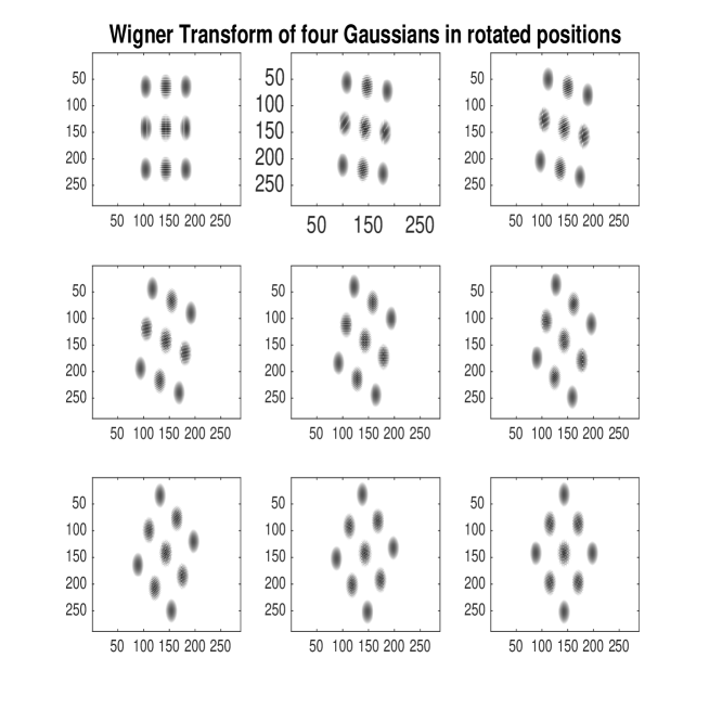
Figure 1. Wigner transform, logarithmic amplitude

4. Symplectic covariance for the Cohen class

A quadratic time-frequency representation $Q$ belongs to the Cohen’s class if it can be written as

(31) $$Qf=Wf\ast\theta,\quad\forall f\in\mathcal{S}(\mathbb{R}^{n})$$

for a suitable kernel $\theta\in\mathcal{S}^{\prime}({\mathbb{R}^{2n}})$.

Observe that for a distribution in the Cohen’s class, using (7) we have, for every $f\in\mathcal{S}(\mathbb{R}^{n})$,

$$Q(\widehat{T}(z_{0})f)(z) =(W(\widehat{T}(z_{0})f)\ast\theta)(z)=((T(z_{0})Wf)\ast\theta)(z)$$

$$=T(z_{0})(Wf\ast\theta)(z)=T(z_{0})Qf(z).$$

Hence, for every $Q$ in the Cohen’s class, we have the translation formula:

(32) $$Q(\widehat{T}(z_{0})f)(z)=Qf(z-z_{0}),$$

as for the Wigner distribution.

Let us now study the behaviour of the Cohen’s class under the action of metaplectic operators.

Proposition 4.1 (Symplectic covariance of the Cohen’s class).

Consider $\theta\in\mathcal{S}^{\prime}(\mathbb{R}^{n})$ and $Q$ an element of the Cohen’s class having kernel $\theta$, as in (31). For $\widehat{S}\in Mp(n,\mathbb{R})$ and $S=\pi^{Mp}(\widehat{S})$, we have

(33) $$Q(\widehat{S}f)(z)=Wf\ast(\theta\circ S)(S^{-1}z),\quad\forall f\in\mathcal{S}(\mathbb{R}^{n}),\quad z\in{\mathbb{R}^{2n}}.$$

Proof.

Recalling the symplectic covariance for the Wigner distribution (Theorem 2.2)

$$W(\widehat{S}f)(z)=Wf(S^{-1}z),\quad f\in\mathcal{S}(\mathbb{R}^{n}),\quad z\in{\mathbb{R}^{2n}},$$

we can write, for any $f\in\mathcal{S}(\mathbb{R}^{n})$,

$$Q(\widehat{S}f)(z) =(W(\widehat{S}f)\ast\theta)(z)$$

$$=\int_{{\mathbb{R}^{2n}}}W(\widehat{S}f)(z-w)\theta(w)\,dw$$

$$=\int_{{\mathbb{R}^{2n}}}Wf(S^{-1}(z-w))\theta(w)\,dw$$

$$=\int_{{\mathbb{R}^{2n}}}Wf(u)\theta(z-Su)\,du$$

$$=\int_{{\mathbb{R}^{2n}}}Wf(u)\theta(S(S^{-1}z-u))\,du$$

$$=Wf\ast(\theta\circ S)(S^{-1}z)$$

where the integrals must be understood in the sense of distributions (we recall that $Wf\in\mathcal{S}({\mathbb{R}^{2n}})$ for $f\in\mathcal{S}(\mathbb{R}^{n})$, cf. [16, Theorem 11.2.5]). Moreover, in the change of variables we used $\det S=1$.       

As a consequence, we recover the results for the covariance of the Born–Jordan distribution in [10].

Corollary 4.2.

If $\theta=\theta_{\mathrm{BJ}}$ as in (11), we have the covariance of the corresponding distribution $Q$ for all the symplectic matrices of the type $S=J$ or $S=M_{L}=\begin{pmatrix}L^{-1}&0\\ 0&L^{t}\end{pmatrix}$, with $L\in\mathrm{GL}(2n,\mathbb{R})$.

The covariance behavior of the Born–Jordan distribution is illustrated in Figure 2, for the same set of rotated superposition of quantum states we considered in the previous section. We observe that the interference terms depend substantially on the underlying coordinate system. In particular, choosing an appropriate rotation, the interference terms can be significantly damped.

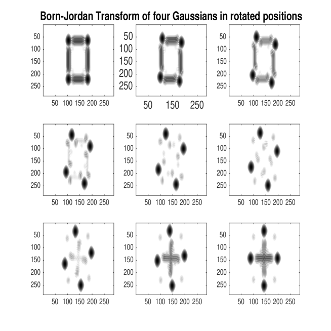
Figure 2. Born-Jordan transform, logarithmic amplitude

Formula (33) motivates the investigations of the temperate distributions which are invariant with respect to the action of the linear symplectic group. We need the following easy lemma.

Lemma 4.3.

Let $\theta\in\mathcal{S}^{\prime}({\mathbb{R}^{2n}})$ and $A$ be a square $2n\times 2n$ real matrix. We have

(34) $$\frac{\mathrm{d}}{\mathrm{dt}}\theta(e^{tA}z)|_{t=0}=Az\cdot\nabla_{z}\theta.$$

Proof.

We have, for $\varphi\in\mathcal{S}({\mathbb{R}^{2n}})$,

(35) $$\langle\frac{1}{t}\big{(}\theta(e^{tA}\cdot)-\theta\big{)},\varphi\rangle=\langle\theta,\frac{1}{t}\big{(}e^{-t\,\mathrm{Tr}\,A}\varphi(e^{-tA}\cdot)-\varphi\big{)}\rangle.$$

Now, as $t\to 0$ we have

$$\frac{1}{t}\big{(}e^{-t\,\mathrm{Tr}\,A}\varphi(e^{-tA}\cdot)-\varphi\big{)}\to-\mathrm{Tr}\,A\,\varphi-Az\cdot\nabla_{z}\varphi$$

in $\mathcal{S}({\mathbb{R}^{2n}})$, so that the left-hand side in (35) tends to

$$\langle\theta,-\mathrm{Tr}\,A\,\varphi-Az\cdot\nabla_{z}\varphi\rangle =\langle-\mathrm{Tr}\,A\,\theta+\mathrm{div}\big{(}Az\,\theta\big{)},\varphi\rangle$$

$$=\langle Az\cdot\nabla_{z}\theta,\varphi\rangle.$$

      

Proposition 4.4.

Let $\theta\in\mathcal{S}^{\prime}({\mathbb{R}^{2n}})$ be such that

$$\theta\circ S=\theta$$

for every $S\in\mathrm{Sp}(n,\mathbb{R})$. Then

$$\theta=c_{0}+c_{1}\delta$$

for some $c_{0},c_{1}\in\mathbb{C}$.

Proof.

It suffices to consider the case where $S=e^{A}$ with $A\in\mathfrak{sp}(n,\mathbb{R})$ (the symplectic algebra, i.e. the Lie algebra of $\mathrm{Sp}(n,\mathbb{R})$). Consider the one-parameter group of symplectic matrices $e^{tA}\in\mathrm{Sp}(n,\mathbb{R})$, $t\in\mathbb{R}$. The assumption $\theta\circ S=\theta$ implies that

$$\theta(e^{tA}z)=\theta(z)$$

for every $A\in\mathfrak{sp}(n,\mathbb{R})$ and therefore

$$\frac{\mathrm{d}}{\mathrm{dt}}\theta(e^{tA}z)=0.$$

On the other hand, by Lemma 4.3, we have

(36) $$\frac{\mathrm{d}}{\mathrm{dt}}\theta(e^{tA}z)|_{t=0}=Az\cdot\nabla_{z}\theta$$

and therefore

(37) $$Az\cdot\nabla_{z}\theta=0\quad\forall A\in\mathfrak{sp}(n,\mathbb{R}).$$

Now, for $z\not=0$ fixed, we have

(38) $$\mathcal{T}_{z}=\{Az:\ A\in\mathfrak{sp}(n,\mathbb{R})\}={\mathbb{R}^{2n}},\quad z\not=0.$$

In fact $\mathcal{T}_{z}\simeq\{Az\cdot\nabla_{z}:\ A\in\mathfrak{sp}(n,\mathbb{R})\}$ is the tangent space at $z$ to the orbit of the action of $\mathrm{Sp}(n,\mathbb{R})$ on ${\mathbb{R}^{2n}}\setminus\{0\}$. Since the action is transitive, the orbit is the whole ${\mathbb{R}^{2n}}\setminus\{0\}$, and (38) follows.

As a consequence of (37) and (38) we have $\nabla_{z}\theta=0$ in ${\mathbb{R}^{2n}}\setminus\{0\}$, and therefore $\theta=c_{0}$ in ${\mathbb{R}^{2n}}\setminus\{0\}$. The distribution $\theta-c_{0}$ in ${\mathbb{R}^{2n}}$ is supported at $0$, so that

(39) $$\theta=c_{0}+c_{1}\delta+\sum_{1\leq|\alpha|\leq m}c^{\prime}_{\alpha}\partial^{\alpha}_{z}\delta$$

for some $m\geq 1$, $c^{\prime}_{\alpha}\in\mathbb{C}$. We have to show that in fact the summation in (39) is zero. To this end we observe that, taking the Fourier transform of both sides of the invariance property $\theta\circ S=\theta$, $S\in\mathrm{Sp}(n,\mathbb{R})$, we see that $\widehat{\theta}$ enjoys the same invariance, so that by the above argument we have

$$\widehat{\theta}=c_{2}+v,$$

for some $c_{2}\in\mathbb{C}$, $v\in\mathcal{S}^{\prime}({\mathbb{R}^{2n}})$ supported at $0$. This is compatible with (39) only if the summation in (39) is zero.       

Remark 4.5.

An inspection of the above proof shows that we only need invariance with respect to the symplectic matrices of the form $e^{tA}$, with $a\in A\in\mathfrak{sp}(n,\mathbb{R})$ and small $t$. However, this condition turns out to be equivalent to the invariance with respect to the full symplectic group, because any connected Lie group is generated by a neighborhood of the identity.

We now prove the characterization of the Wigner transform announced in Introduction. For a quadratic map $Q$ we denote by $Q(f,g)$ its corresponding sesquilinear map.

Theorem 4.6.

Consider a quadratic continuous time-frequency distribution $Q:L^{2}(\mathbb{R}^{n})\to C_{0}({\mathbb{R}^{2n}})$, i.e. $Qf=Q(f,f)$ for a sequilinear continuous map $Q:L^{2}(\mathbb{R}^{n})\times L^{2}(\mathbb{R}^{n})\to C_{0}({\mathbb{R}^{2n}})$. Suppose that $Q$ enjoys:

(i) the covariance property with respect to translations in the time-frequency plane:

(40) $$Q(\widehat{T}(z_{0})f)(z)=Qf(z-z_{0}),\quad\forall f\in\mathcal{S}(\mathbb{R}^{n}),\ z_{0}\in\mathbb{R}^{2n};$$

(ii) the covariance property with respect to symplectic linear transformations: for every $\widehat{S}\in\mathrm{Mp}(n,\mathbb{R})$, with $S=\pi^{\mathrm{Mp}}(\widehat{S})\in\mathrm{Sp}(n,\mathbb{R})$

(41) $$Q(\widehat{S}f)(z)=Qf(S^{-1}z),\quad\forall f\in\mathcal{S}(\mathbb{R}^{n}),\ z\in\mathbb{R}^{2n}.$$

Then

$$Qf=c\,Wf$$

for some constant $c\in\mathbb{C}$.

Proof.

It follows from [16, Theorem 4.5.1] that the continuity assumption

$$|Q(f,g)(z)|\leq C\|f\|_{L^{2}(\mathbb{R}^{n})}\|g\|_{L^{2}(\mathbb{R}^{n})},\quad\forall f,g\in\mathcal{S}(\mathbb{R}^{n}),\ z\in{\mathbb{R}^{2n}}$$

together with (40) imply that

$$Qf=Wf\ast\theta,\quad\forall f\in\mathcal{S}(\mathbb{R}^{n})$$

for some distribution $\theta\in\mathcal{S}^{\prime}({\mathbb{R}^{2n}})$, i.e. $Q$ is a distribution in the Cohen class.

Using this expression for $Q$, together with (33) and (41) we get

$$Wf\ast(\theta\circ S)(S^{-1}z)=Wf\ast\theta(S^{-1}z),\quad\forall f\in\mathcal{S}(\mathbb{R}^{n}),\ \forall z\in{\mathbb{R}^{2n}}.$$

Replacing $S^{-1}z$ by $z$ and taking the Fourier transform we get

$$\widehat{Wf}\,\widehat{\theta\circ S}=\widehat{Wf}\,\widehat{\theta},\quad\forall f\in\mathcal{S}(\mathbb{R}^{n}).$$

If $f$ is a Gaussian function in $\mathbb{R}^{n}$, $\widehat{Wf}$ will be a Gaussian itself in ${\mathbb{R}^{2n}}$, and in particular never vanishes. Hence we obtain $\theta\circ S=\theta$ for every $S\in\mathrm{Sp}(n,\mathbb{R})$. From Proposition 4.4 we have $\theta=c_{0}+c_{1}\delta$ for some $c_{0},c_{1}\in\mathbb{C}$. Finally, since the distribution $Qf=Wf\ast\theta$ is assumed to tend to $0$ at infinity, for every $f\in\mathcal{S}(\mathbb{R}^{n})$, it must be $c_{0}=0$ and we obtain the desired result.       

We now provide a similar characterization for the Weyl transform. We begin by characterizing the transform which enjoy a covariance property with respect to time-frequency shifts, alias Heisenberg operators $\widehat{T}(z_{0})$.

Theorem 4.7.

Consider a linear continuous mapping

$$\mathcal{S}^{\prime}({\mathbb{R}^{2n}})\to\mathcal{L}(\mathcal{S}(\mathbb{R}^{n}),\mathcal{S}^{\prime}(\mathbb{R}^{n})),$$

say $a\longmapsto A_{a}$, satisfying the covariance property with respect to the Heisenberg operators:

(42) $$\widehat{T}(-z_{0})A_{a}\widehat{T}(z_{0})=A_{{T}(-z_{0})a}\quad\forall z_{0}\in{\mathbb{R}^{2n}}.$$

Then there exists a distribution $\theta\in\mathcal{S}^{\prime}({\mathbb{R}^{2n}})$, with $\widehat{\theta}$ smooth in ${\mathbb{R}^{2n}}$, such that

(43) $$\langle A_{a}f,g\rangle=\langle a,W(g,f)\ast\theta\rangle\quad\forall f,g\in\mathcal{S}(\mathbb{R}^{d}).$$

Proof.

By polarization it is sufficient to prove (43) when $f=g$. Now, define the quadratic distribution

$$Qf(z)=\langle A_{a}f,f\rangle,\quad\mathrm{with}\ a(\cdot)=\delta(\cdot-z),\ z\in{\mathbb{R}^{2n}}.$$

By (42) it satisfies the covariance property

$$Q(\widehat{T}(z)f)=T(z)Qf$$

so that it follows from [16, Theorem 4.5.1] (or better from its proof) that there exists a distribution $\theta\in\mathcal{S}^{\prime}({\mathbb{R}^{2n}})$ such that

$$Qf=Wf\ast\theta.$$

This proves (43) when $a(\cdot)=\delta(\cdot-z)$, $z\in{\mathbb{R}^{2n}}$.

Now, let $\mathcal{L}$ be the linear span of such symbols in $\mathcal{S}^{\prime}({\mathbb{R}^{2n}})$. Since the left-hand side of (43) is continuous as a functional of $a\in\mathcal{S}^{\prime}({\mathbb{R}^{2n}})$, for fixed $f,g\in\mathcal{S}({\mathbb{R}^{2n}})$, we see that the right-hand side extends to a continuous functional $\mathcal{S}^{\prime}({\mathbb{R}^{2n}})\to\mathbb{C}$, i.e. there exists a Schwartz function $b\in\mathcal{S}({\mathbb{R}^{2n}})$ such that

$$\langle a,W(g,f)\ast\theta\rangle=\langle a,b\rangle\quad\forall a\in\mathcal{L}$$

that is $W(g,f)\ast\theta=b$ is a Schwartz function. Hence the right-hand side of (43) is also continuous $\mathcal{S}^{\prime}({\mathbb{R}^{2n}})\to\mathbb{C}$, as a functional of $a$, and therefore (43) holds not only for $a\in\mathcal{L}$ but for every $a\in\mathcal{S}^{\prime}({\mathbb{R}^{2n}})$, because $\mathcal{L}$ is dense in $\mathcal{S}^{\prime}({\mathbb{R}^{2n}})$ (cf. [14, Lemma 7]).

Finally, we have already proved that $W(g,f)\ast\theta$, and therefore $\widehat{W(g,f)}\widehat{\theta}$, is a Schwartz function. For suitable fixed Schwartz functions $f=g$ (e.g. a Gaussian) we have $\widehat{Wf}(w)\not=0$ for every $w\in{\mathbb{R}^{2n}}$, which implies that the distribution $\widehat{\theta}$ is in fact smooth in ${\mathbb{R}^{2n}}$.       

As a consequence of these results we obtain the following new characterization of the Weyl transform.

Theorem 4.8.

Consider a linear continuous mapping

$$\mathcal{S}^{\prime}({\mathbb{R}^{2n}})\to\mathcal{L}(\mathcal{S}(\mathbb{R}^{n}),\mathcal{S}^{\prime}(\mathbb{R}^{n})),$$

say $a\longmapsto A_{a}$, satisfying

(i) the covariance property (42) with respect to Heisenberg operators;

(ii) the covariance property with respect to metaplectic operators: for $\widehat{S}\in{\mathrm{M}p}(n,\mathbb{R})$ and $S=\pi^{Mp}(\widehat{S})\in\mathrm{Sp}(n,\mathbb{R})$,

(44) $$\widehat{S}^{-1}A_{a}\widehat{S}=A_{a\circ S}.$$

Then, for some $c\in\mathbb{C}$ we have

(45) $$\langle A_{a}f,g\rangle=c\langle a,W(g,f)\rangle\quad\forall f,g\in\mathcal{S}(\mathbb{R}^{n}).$$

If in addition we have $A_{a}=I$ for $a=1$, then $c=1$ in (45).

Proof.

Again by polarization it is sufficient to prove (45) for $f=g$.

By Theorem 4.7 we have

(46) $$\langle A_{a}f,f\rangle=\langle a,Wf\ast\theta\rangle\quad\forall f,g\in\mathcal{S}(\mathbb{R}^{d})$$

for some distribution $\theta\in\mathcal{S}^{\prime}({\mathbb{R}^{2n}})$ with $\widehat{\theta}$ smooth in ${\mathbb{R}^{2n}}$. Let $Qf:=Wf\ast\theta$. We have therefore, by Proposition 4.1,

$$\langle A_{a}\widehat{S}f,\widehat{S}f\rangle=\langle a,Q(\widehat{S}f)\rangle=\langle a,[Wf\ast(\theta\circ S)]\circ S^{-1}\rangle.$$

On the other hand, using (ii) we have

$$\langle A_{a}\widehat{S}f,\widehat{S}g\rangle=\langle a\circ S,Qf\rangle=\langle a,Qf\circ S^{-1}\rangle.$$

Hence it must be $Wf\ast\theta=Wf\ast(\theta\circ S)$ for every $f\in\mathcal{S}(\mathbb{R}^{n})$. As in the proof of Theorem 4.6 we deduce that $\theta\circ S=\theta$ for every $S\in{\mathrm{S}p}(n,\mathbb{R})$. Proposition 4.4 implies that $\theta=c_{0}+c_{1}\delta$, for some $c_{0},c_{1}\in\mathbb{C}$, but $\widehat{\theta}$ is smooth in ${\mathbb{R}^{2n}}$, so that $c_{0}=0$. We have therefore $\theta=c\delta$ in (46), which gives (45).

The last part of the statement is clear, because $\langle f,g\rangle=\langle 1,W(g,f)\rangle$.       

Remark 4.9.

The result in Theorem 4.8 can be compared with the known characterization of the Weyl transform. Is is proved in [23, Sections 7.5-7.6, pages 578-579] and [26, Theorem 30.2] that the conclusion of Theorem 4.8 holds (with $c=1$) if one assumes

(i)’ $A_{a}f=af$ for $a=a(x)\in L^{\infty}(\mathbb{R}^{n})$

and (ii).

We emphasize that, instead, in Theorem 4.8, (i) and (ii) together amount to assuming the covariance with respect to the extended symplectic group.

References

• [1] P. Boggiatto, G. De Donno, A. Oliaro, Time-Frequency Representations of Wigner Type and Pseudo-Differential Operators, Trans. Amer. Math. Soc., 362(9) (2010) 4955–4981.
• [2] M. Born, P. Jordan, Zur Quantenmechanik, Z. Physik 34 (1925) 858–888.
• [3] M. Born, W. Heisenberg, P. Jordan, Zur Quantenmechanik II, Z. Physik 35 (1925) 557–615.
• [4] L. Cohen, Generalized phase-space distribution functions. J. Math. Phys. 7 (1966) 781–786.
• [5] L. Cohen, The Weyl operator and its generalization, Springer Science & Business Media, 2012.
• [6] E. Cordero, M. de Gosson, and F. Nicola, On the invertibility of Born–Jordan quantization. J. Math. Pures Appl. 105 (2015) 537–557.
• [7] E. Cordero, M. de Gosson, F. Nicola, On the reduction of the interferences in the Born-Jordan quantization, Appl. Comp. Harm. Anal., to appear (available at arXiv:1601.03719).
• [8] M. de Gosson, Symplectic Geometry and Quantum Mechanics. Birkhäuser, Basel, series “Operator Theory: Advances and Applications” (subseries: “Advances in Partial Differential Equations”), Vol. 166, 2006.
• [9] M. de Gosson, Symplectic Methods in Harmonic Analysis and in Mathematical Physics, Birkhäuser, 2011.
• [10] M. de Gosson, Symplectic Covariance properties for Shubin and Born–Jordan Pseudo-differential operators. Trans. Amer. Math. Soc., 365(6) (2013) 3287–3307.
• [11] M. de Gosson, Born–Jordan Quantization and the Equivalence of the Schrödinger and Heisenberg Pictures. Found. Phys. 44(10) (2014) 1096–1106.
• [12] M. de Gosson, Born-Jordan Quantization: Theory and Applications., Springer 2016
• [13] M. de Gosson, F. Luef, Preferred Quantization Rules: Born–Jordan vs. Weyl; Applications to Phase Space Quantization. J. Pseudo-Differ. Oper. Appl. 2(1) (2011) 115–139.
• [14] M. de Gosson and F. Nicola, Born-Jordan Pseudodifferential Operators and the Dirac Correspondence: Beyond the Groenewold-van Hove Theorem, arXiv:1606.07796.
• [15] G. B. Folland, Harmonic Analysis in Phase Space. Princeton Univ. Press, Princeton, NJ, 1989.
• [16] K. Gröchenig, Foundation of Time-Frequency Analysis, Birkhäuser, Boston MA, 2001.
• [17] F. Hlawatsch, Interference terms in the Wigner distribution.Digital signal processing 84 (1984) 363–367.
• [18] F. Hlawatsch and P. Flandrin, The interference structure of the Wigner distribution and related time-frequency signal representations. The Wigner Distribution – Theory and Applications in Signal Processing (1997) 59–133.
• [19] L. Hörmander, The analysis of linear partial differential operators I, Grundl. Math. Wissenschaft. 256, Springer, 1985.
• [20] N. H. McCoy, On the function in quantum mechanics which corresponds to a given function in classical mechanics, Proc. Natl. Acad. Sci. U.S.A. 18(11) (1932) 674–676.
• [21] H. Oehlmann and D. Brie, The reduced-interference local Wigner-Ville distribution. In ICASSP-97 (IEEE International Conference on Acoustics, Speech, and Signal Processing), 1997.
• [22] S.Pikula and P. Benes, A New Method for Interference Reduction in the Smoothed Pseudo Wigner-Ville Distribution. In Proceedings of the 8th International Conference on Sensing Technology, Sep. 2-4, 2014, Liverpool, UK
• [23] E. M. Stein, Harmonic Analysis: Real Variable Methods, Orthogonality, and Oscillatory Integrals, Princeton University Press, 1993
• [24] V. Turunen, Born-Jordan time-frequency analysis. To appear in RIMS Kôkyûroku Bessatsu B56, Res. Inst. Math. Sci. (RIMS), Kyoto, 2016.
• [25] H. Weyl, Quantenmechanik und Gruppentheorie, Zeitschrift für Physik 46 (1927).
• [26] M. W. Wong, Weyl Transforms, the Heat Kernel and Green Function of a Degenerate Elliptic Operator, Annals Global Anal. Geom. 28 (2005) 271–283
• [27] W. H. Zurek, Sub-Planck structure in phase space and its relevance for quantum decoherence. Nature 412(6848) (2001) 712–717.