Differences between radio-loud and radio-quiet $\gamma-$ray pulsars as revealed by Fermi

Abstract

By comparing the properties of non-recycled radio-loud $\gamma-$ray pulsars and radio-quiet $\gamma-$ray pulsars, we have searched for the differences between these two populations. We found that the $\gamma-$ray spectral curvature of radio-quiet pulsars can be larger than that of radio-loud pulsars. Based on the full sample of non-recycled $\gamma-$ray pulsars, their distributions of the magnetic field strength at the light cylinder are also found to be different. We notice that this might be resulted from the observational bias. In re-examining the previously reported difference of $\gamma-$ray-to-X-ray flux ratios, we found the significance can be hampered by their statistical uncertainties. In the context of outer gap model, we discuss the expected properties of these two populations and compare with the possible differences identified in our analysis.

1 Introduction

Before the launch of Fermi $\gamma-$ray Space Telescope, our understanding of $\gamma-$ray pulsars was very limited. Its predecessor Compton Gamma-Ray Observatory (CGRO) has only detected seven pulsars in MeV-GeV regime throughout its almost nine years life-time (Thompson 2008). Among them, there is a special member, Geminga (PSR J0633+1746), which was the only known radio-quiet $\gamma-$ray pulsar in the pre-Fermi era (see Bignami & Caraveo 1996 for a review).

With its much improved sensitivity and accurate source localization, the Large Area Telescope (LAT) onboard Fermi has expanded the $\gamma-$ray pulsar population considerably shortly after its operation (Abdo et al. 2009a,b). 16 new $\gamma-$ray pulsars have been discovered through blind searches with just $\sim 4.5$ month data (Abdo et al. 2009a). Currently, there are 205 $\gamma-$ray pulsars have been detected by LAT.

In the second Fermi LAT pulsar catalog (2PC Abdo et al. 2013), the detailed properties of 117 pulsars detected at energies $>100$ MeV with three years data are reported. It comprises 42 radio-loud pulsars, 35 radio-quiet pulsars and 40 millisecond pulsars (Abdo et al. 2013).

Establishing radio-quiet $\gamma-$ray pulsars as a definite class is one of the triumphs of Fermi. Different from the radio-loud cases, they can only be detected through blind pulsation searches at high energies. Apart from the high sensitivity of LAT, the expansion of radio-quiet pulsar population also thanks to the improvement of searching techniques (e.g. Kerr 2011).

About 30$\%$ of the known $\gamma-$ray pulsars are radio-quiet. Taking the selection effects into account, this fraction can be even larger. Sokolova & Rubtsov (2016) have estimated that the intrinsic fraction of radio-quiet $\gamma-$ray pulsars can be as large as $\sim 70\%$. Such large fraction of radio-quietness imposes strict constraints on the geometry and mechanism of the pulsar emission. This implies the $\gamma-$rays are originated from the outer magnetosphere and form a fan beam (see Cheng & Zhang 1998; Takata et al. 2006, 2008). In comparison with the narrow cone-like radio beam originated from the polar cap region, this makes the detection of $\gamma-$ray pulsation less sensitive to the emission and viewing geometry.

As the sample sizes of radio-quiet $\gamma-$ray pulsars and the non-recycled radio-loud $\gamma-$ray pulsars are now comparable, a deeper insight of their nature can be gained by comparing their physical and emission properties. Marelli et al. (2011,2015) and Marelli (2012) have shown that the $\gamma-$ray-to-X-ray flux ratios of radio-quiet population are higher than that of radio-loud ones. While these works did not found any solid evidence for the difference between these two populations neither in terms of the physical properties (e.g. magnetic field) nor in $\gamma-$ray regime, Marelli et al. (2015) suggest this implies the X-ray emission of the radio-quiet population is generally fainter. The authors further speculated that this might be due to a luminous X-ray emission component from the polar caps of radio-quiet pulsars missing the line-of-sight. Recently, Sokolova & Rubtsov (2016) have also reported their attempt in searching the difference between radio-loud and radio-quiet populations. No significant differences in their ages and locations in the Galaxy have been found. On the other hand, there is a possible difference between their distributions of rotation period.

The aforementioned studies have shown that the properties of radio-loud and radio-quiet $\gamma-$ray pulsars can be intrinsically different. However, a thorough comparison of other characteristics of pulsars, such as magnetic field strength and spectral properties, remains unreported. This motivates us to perform a systematic search for the difference of the emission and physical properties between these two populations through a detailed statistical analysis.

2 Data Analysis

All the data used in this work are collected from 2PC (Abdo et al. 2013) and the third Fermi $\gamma-$ray point sources catalog (3FGL; Acero et al. 2015), which are summarized in Table 1 and Table 2. These parameters are chosen to characterize the pulsars in the following aspects:

1. Magnetic field strength and spin-down power - Magnetic field strength is a crucial factor for the acceleration and emission processes in the magnetosphere (e.g. Cheng & Zhang 1998). In this work, we compare the magnetic field of radio-loud and radio-quiet populations at the stellar surface $B_{\rm s}$ as well as at the light cylinder $B_{\rm LC}$. Their strength can be derived from the spin period $P$ and its first time derivative $\dot{P}$ as $B_{\rm s}=(2\pi)^{-1}(1.5Ic^{3}P\dot{P})^{1/2}R_{\rm NS}^{-3}$ and $B_{\rm LC}=4\pi^{2}(1.5I\dot{P})^{1/2}(c^{3}P^{5})^{-1/2}$ respectively by assuming a dipolar field geometry, where $I$, $R_{\rm NS}$ and $c$ are moment of inertia, stellar radius and the speed of light. We assume $I=10^{45}$ g cm² and $R_{\rm NS}=10$ km throughout this work.

   We also compare the spin-down power $\dot{E}=4\pi^{2}I\dot{P}P^{-3}$ between these two populations. As the rotational energy of a neutron star provides the reservoir for the pulsar emission, both $\gamma-$ray and X-ray luminosities are found to be scaled with $\dot{E}$ (e.g. Abdo et al. 2013; Possenti et al. 2002).

2. Emission and spectral properties - The $\gamma-$ray spectra of pulsars are typically modeled by a form of a power-law with an exponential cut-off (PLE). The spectral shape of this model is characterized by two parameters, namely the photon index $\Gamma$ and the cut-off energy $E_{\rm cut}$. Such model is curved in comparison with a simple power-law (PL). The spectral curvature of the pulsars are quantified by the parameter Curve$\_$Significance in 3FGL, which are obtained by comparing the difference between the PLE and PL mode fittings (in unit of $\sigma$).

   Apart from comparing these spectral parameters between the radio-loud and radio-quiet population, we also compare their $\gamma-$ray-to-X-ray flux ratios $F_{\gamma}/F_{x}$. Although Marelli et al. (2015) have already pointed out the distributions of $F_{\gamma}/F_{x}$ are different between these two populations, an investigation of its possible correlation with other parameters such as $\dot{E}$ remains unreported. In this study, we will not consider the $\gamma-$ray luminosities of pulsars as they depends on the distances which have a large uncertainties, in particular for the radio-quiet population.

3. Temporal properties - The viewing geometry (i.e. the angle between the line-of-sight and the $\gamma-$ray emission regions) can possibly be different between these two populations. This can possibly be reflected in their pulse profiles. Different viewing geometry can lead to either be a large pulse width (FWHM) for the single peak cases or a large peak separation for the multiple peaks cases ($\Delta_{\gamma}$), depending on whether the line-of-sight cut through a single emission region or a multiple emission regions. This motivates us to compare the combined distributions of FWHM and $\Delta_{\gamma}$ between these two populations.

   One of the radio-quiet pulsars PSR J2021+4026 has its $\gamma-$ray flux at energies $>100$ MeV suddenly decreased by $\sim 18\%$ near MJD 55850 (Allafort et al. 2013). This makes it to be the first variable $\gamma-$ray pulsar has ever been observed. To investigate whether there is any difference between radio-quiet and radio loud populations in terms of the flux variability, we also compare their distributions of the parameter Variability$\_$Index in 3FGL. This parameter indicates the difference between the light curve of a source and its average flux level over the full time coverage in 3FGL (Acero et al. 2015). For a Variability$\_$Index larger than 72.44, the null hypothesis of a source being steady can be rejected at $99\%$ confidence level (Acero et al. 2015).

2.1 Anderson-Darling Test

The histograms and the cumulative distributions of the chosen parameters are shown in Figure 1 and Figure 2 respectively. For searching the possible differences between the radio-loud and radio-quiet populations, we apply the non-parametric two-sample Anderson-Darling (A-D) test (Anderson & Darling 1952; Darling 1957; Pettitt 1976, Scholz & Stephens 1987) to their unbinned distributions (Figure 2).

While Kolmogorov-Smirnov (K-S) test has been widely used to test whether two unbinned distributions are different, it is not sensitive to identify the difference locates at the edges of the distributions or when these two distributions are crossed.. In view of this, we adopt A-D test in our analysis. Another advantage of A-D test over K-S test is the evidence that it is better capable of detecting small differences (Engmann & Cousineau 2011). In this work, we perform the two-sample A-D test with the code implemented in scipy. The results are summarized in Table 3.

Among all the tested parameters, their distributions of Curve$\_$Significance are found to be the most incompatible ($p-$value$\sim 0.0002$). This indicates the possible difference of their $\gamma-$ray spectral shape.

For comparing their flux ratios $F_{\gamma}/F_{x}$, we omitted all the upper-limits in Tab. 1 and Tab. 2. A difference is found ($p-$value $\sim 0.0005$), which is consistent with the conclusion reported by Marelli et al. (2015) based on comparing their binned histograms.

Another interesting result comes from comparing the magnetic fields of these two populations. While we do not find any difference of surface field strength $B_{\rm S}$ between radio-loud and radio-quiet pulsars, the distributions of the magnetic field at the light cylinder $B_{\rm LC}$ are found to be different ($p-$value$\sim 0.002$; see Fig. 1 & 2).

The statistical significances of the aforementioned differences are $\gtrsim 3\sigma$. However, these results have not taken the uncertainties of the parameters into account. For the $F_{\gamma}/F_{x}$ reported by 2PC, their statistical uncertainties are rather large. The average percentage error is $\sim 34\%$ and $\sim 28\%$ in the radio-loud and radio-quiet populations respectively. Taking this into consideration, the difference of $F_{\gamma}/F_{x}$ between these two populations can be drastically reduced. Shifting their cumulative distributions within the tolerence of their statistical uncertainties, the difference can possibly be reconciled ($p-$value$\sim 0.03$).

For $B_{\rm LC}$, we estimate the uncertatinties by propagating the errors of $P$ and $\dot{P}$ reported in 2PC or the ATNF catalog (Manchester et al. 2005). The mean percentage errors of $B_{\rm LC}$ of radio-loud and radio-quiet populations are $\sim 0.14\%$ and $\sim 0.08\%$ respectively. In view of their small uncertainties, the statistical significance for the difference of $B_{\rm LC}$ between these two populations remains unaltered.

In 3FGL, there is no error estimate for Curve$\_$Significance. However, the accuracy of this parameter depends on how well the $\gamma-$ray spectra can be constrained so that one can discriminate whether PL or PLE models provide a better fit. This in turns depends on the photon statistics. Since radio-loud $\gamma-$ray pulsars can be more easily detected with the aid of their radio ephemeris, their detection significances are generally lower than that of radio-quiet $\gamma-$ray pulsars (see Tab. 1 and 2). Since it is more difficult to detect the faint pulsars at energies higher than the cut-off energy, this might lead to their apparently flatter spectra. In order to test the robustness for the difference of Curve$\_$Significance between these two populations, we alleviate this possible selection effect by re-running the A-D test on the pulsars detected at a level $>10\sigma$ (i.e. $TS>100$ in 3FGL). While all the radio-quiet pulsars satisfy this criteria, this reduces the sample size of the radio-loud pulsars to 29. In this case, the statistical significance for the difference of Curve$\_$Significance is reduced but remains marginally at a $\sim 3\sigma$ level ($p-$value$\sim 0.003$).

We also considered if there is any selection effect can result in the observed difference in $B_{\rm LC}$. $B_{\rm LC}$ is a function of $P$ and $\dot{P}$. To investigate if the difference in $B_{\rm LC}$ is caused by the distributions of their rotational parameters, we have also applied the A-D test seperately on $P$ and $\dot{P}$. In the full sample, we have found a marginal difference of $P$ between this two populations ($p-$value$\sim 0.006$). On the other hand, we do not find any difference in the distributions of $\dot{P}$ ($p-$value$\sim 0.2$). However, we note that the difference in $P$ can possibly be a result of observational bias. For example, radio-loud pulsars can be found with their radio ephemeris. This might facilitate the detection of fast rotation. Attempting to alleviate such effect, Sokolova & Rubtsov (2016) have constructed a bias-free sample by performing blind pulsar searches from all point sources in 3FGL using only LAT data. To estimate the impact of this possible selection effect in $P$ and $B_{LC}$, we re-run the A-D test on the pulsars (26 radio-quiet; 14 radio-loud) detected in the blind search by Sokolova & Rubtsov (2016). We found that the statistical significance for the difference in $P$ is not undermined ($p-$value$\sim 0.006$). For $B_{LC}$, we found the statistical significance for the difference between two populations may drop to the level of $\sim 2.5\sigma$ ($p-$value$\sim 0.01$).

2.2 Correlation & Regression Analysis

In §2.1, we have shown the possible differences between radio-loud and radio-quiet pulsars in terms of $F_{\gamma}/F_{x}$, Curve$\_$Significance and $B_{\rm LC}$. In order to test if there is any relation between the emission properties ($F_{\gamma}/F_{x}$,Curve$\_$Significance) and $B_{\rm LC}$ in each population. We proceed to perform the correlation analysis

From Figure 1, it is obvious that the distributions for most of these parameters do not resemble a Gaussian. In view of this, we adopt a non-parametric approach by computing the Spearman rank coefficients (Conover 1999; Siegel & Castellan 1988). 2PC has also reported a possible correlation between the cut-off energy $E_{\rm cut}$ and $B_{\rm LC}$ for the radio-quiet $\gamma-$ray pulsars (Abdo et al. 2013). However, the authors have adopted a linear correlation analysis (i.e Pearson’s $r$, Fisher 1944) which implicitly assumes $E_{\rm cut}$ and $B_{\rm LC}$ follow a bivariate Gaussian probability distribution. Such assumption is unlikely to be satisfied (cf. Fig. 1). Therefore, we have also run the non-parametric correlation analysis for $E_{\rm cut}-B_{\rm LC}$ to cross-check this possible relation. The results are summarized in Table 4.

For $F_{\gamma}/F_{x}$ and Curve$\_$Significance, we do not find any evidence for the correlation with $B_{\rm LC}$ in both radio-loud and radio-quiet populations. On the other hand, for the radio-quiet pulsars, $E_{\rm cut}$ is found to have a strong positive correlation with $B_{\rm LC}$ ($p-$value $\sim 2\times 10^{-6}$) However, this relation cannot be found in the radio-loud population ($p-$value $\sim 0.1$).

We further examine the phenomenological relation $E_{\rm cut}-B_{\rm LC}$ in the case of radio-quiet pulsars by assuming a linear model $E_{\rm cut}=a+b\log B_{\rm LC}$ in a regression analysis. The best-fit model is:

$$E_{\rm cut}=(-1.74\pm 0.36)+(1.15\pm 0.11)\log B_{\rm LC}~{}{\rm GeV},$$ (1)

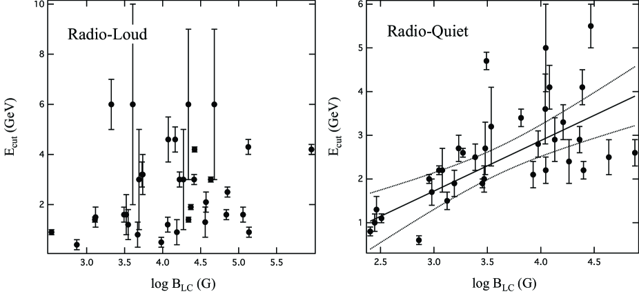
Figure 4: The cut-off energies $E_{\rm cut}$ vs. $B_{\rm LC}$ in radio-loud (left panel) and radio-quiet (right panel) $\gamma-$ray pulsar populations. The solid line in the right panel represent the best-fit from the regression analysis. The dotted lines represent the upper and lower $95\%$ confidence bands.

which is shown in Figure 4. The quoted uncertainties are 95$\%$ confidence intervals. We have also displayed the corresponding plot for the radio-loud pulsars for comparison.

3 Summary & Discussions

We have performed a detailed statistical analysis to probe the physical nature of radio-loud and radio-quiet $\gamma-$ray pulsars. By comparing the cumulative frequency distributions of a set of selected parameters (see Figure 2), we have identified the possible differences between these two populations in several aspects (cf. Table 3). We found that the $\gamma-$ray spectral curvature of radio-quiet pulsars can be larger than that of radio-loud pulsars. While the surface magnetic field strength $B_{\rm s}$ has a similar distribution in both populations, their magnetic field strength at the light cylinder $B_{\rm LC}$ are found to be different. However, we need to point out that the significance can possibly be hampered by the effect of observational selection bias.

In re-examining the distributions of nominal values of $F_{\gamma}/F_{x}$, we confirmed the difference between the radio-loud and radio-quiet pulsars as claimed by Marelli et al. (2015). However, with the large statistical uncertainties of $F_{\gamma}/F_{x}$ taking into account, it does not allow one to draw a firm conclusion on their difference.

While the possible differences identified in our analysis might be suffered from the selection effects and the statistical uncertainties, we note that such differences can be explained in the context of outer gap model by the geometric effect and the rotational period. In the following, we explain these properties qualitatively by assuming: (1) the $\gamma-$rays are originated from the outer gap, (2) the X-rays are originated from the polar cap due to backflow current heating, and (3) the open angle of the radio emission cone depends on $P^{-1/2}$ (e.g. Lyne & Manchester 1988; Kijak & Gil 1998, 2003).

Since $B_{\rm LC}\sim B_{\rm s}P^{-3}$, the differences between radio-loud and radio-quiet populations should stem from the rotational period $P$ (cf. Fig. 3). We noted that $P$ of radio-loud pulsars are generally smaller than radio-quiet pulsars. We first assume all pulsars have radio emission cones. Whether one is radio-loud or radio-quiet, it depends on whether the line-of-sight can meet the radio cone. From radio observations, it has been found that the radio cone size is related to the period of pulsars as $\sim P^{-\alpha}$ (e.g.,Narayan & Vivekanand 1983; Lyne & Manchester 1988; Biggs 1990; Gil, Kijak, & Seiradakis 1993; Gil & Han 1996; Kijak & Gil 1998, 2003), where $\alpha$ is about 0.5. Therefore, shorter period pulsars will have wider radio cone and hence more favorable to be radio-loud. And hence the radio-quietness in the pulsar population might be a result of their narrower radio cones.

Concerning the difference in $F_{\gamma}/F_{x}$, we consider a geometric effect together with assumption that the X-rays are coming from the regions near the polar cap (e.g. Arons 1981; Harding, Ozernoy, & Usov 1993; Cheng, Gil & Zhang 1998; Cheng & Zhang 1999). In this case its intensity $F_{x}^{\rm pc}$ should depend on the angle between the magnetic axis and the viewing angle $\theta$, namely $F_{x}^{\rm pc}\propto\cos\theta$. Based on the assumption that the line-of-sight of the radio-loud pulsars must be within the radio cone and that for radio-quiet pulsars is outside the radio cone, then radio loud pulsars should have smaller $\theta$ than those radio quiet pulsars. This implies the mean $F_{x}$ of radio-loud pulsars is larger than that of the radio-quiet pulsars. From observations and simulations (e.g. Takata, Wang and Cheng 2011), the difference in the $\gamma$-ray flux distributions between radio-loud and radio-quiet pulsars is not very large. On the other hand, $\cos\theta$ can vary from 0 to 1. Assuming $F_{\gamma}$ is similar for these two populations, $F_{\gamma}/F_{x}$ of radio-quiet population should be larger than the radio-loud group.

We note a special pulsar PSR J0537-6910 which is radio-quiet X-ray pulsar but without $\gamma-$ray emission detected (Marshall et al. 1998; Gotthelf et al. 1998). Its X-ray emission is likely to be non-thermal dominant (Gotthelf et al. 1998) which presumably originated from the synchrotron emission of backflow current in the outer gap (cf. Cheng & Zhang 1999). The non-detection of radio emission and the thermal X-ray component imply that our line-of-sight is far from its polar cap region. As the beaming directions of the $\gamma-$rays and the non-thermal X-rays are not necessary in the same direction (cf. Fig. 2 in Cheng & Zhang 1999), our line-of-sight might miss the $\gamma-$ray emitting region as well.

To account for the difference of $\gamma-$ray spectral curvature, we speculate that inverse Compton (IC) process may play a role in high energy photon production. The most natural soft photons are radio. For the radio-loud pulsars, which generally have wider radio cones than their radio-quiet counterparts, part of radio emission with frequency $>100$ MHz may get into the outer gap and IC scatter with the primary electrons/positrons to the photons in GeV regime (cf. Ng et al. 2014). On the other hand, the probability of radio photons in radio-quiet pulsars get into the gap is low. This could lead to a shortage of photons produced at higher energies through the aforementioned IC process. And this might result in more curved spectra of radio-quiet pulsars.

$E_{\rm cut}$ of radio-quiet pulsars are found to be strongly correlated with $B_{\rm LC}$. However, such association is absent in the radio-loud population. The aforementioned IC scenario can also provide a possible way to account for this phenonmena. $E_{\rm cut}$ might be determined by IC scattering between the radio emission and the primary electrons/positrons in the outer gap. Such effect can be enhanced if the open angle of the radio cone is larger. And hence $E_{\rm cut}$ should be proportional to $1/P$ and this results in the positive correlation between $E_{\rm cut}$ and $B_{\rm LC}$. From the histograms (cf. Figure 1), we notice that the spread of $E_{\rm cut}$ is wider in the radio-loud population than that in the radio-quiet population. This might indicate that the factor of determining the cut-off energy is more complicated in the case of radio-loud pulsars.

While the differences between the radio-quiet and radio-loud pulsars reported in this work are physically plausible by the outer gap model, a firm conclusion is limited by the current sample and various observational biases. With more $\gamma-$ray pulsars detected in the future, their properties suggested by our analysis can be re-examined.

Table 1: The selected parameters of radio-loud $\gamma-$ray pulsars as described in the main text of Sec. 2.

PSR	$P$	$\dot{P}$	$B_{S}$	$B_{LC}$	$\dot{E}$	Variability	Curve	$E_{cut}$	$\Gamma$	$F_{\gamma}/F_{X}$	$\Delta_{\gamma}$	FWHM	$TS^{a}$
						Index	Significance
	(ms)	$(10^{-15}$ s/s)	$(10^{10}G)$	(G)	($10^{34}$ erg/s)			(GeV)
J0205+6449	65.7	190	353.3	114617.6	2644	37.4	4.9	$1.6\pm 0.3$	$1.8\pm 0.1$	$29.7\pm 2.1$	$0.503\pm 0.004$	$\cdot\cdot\cdot$	1019
J0248+6021	217.1	55	345.6	3106.8	21.2	66.6	7.1	$1.6\pm 0.3$	$1.8\pm 0.1$	$>57.4$	$\cdot\cdot\cdot$	0.1968	578
J0534+2200	33.6	420	375.7	911096.3	43606	621.9	15.8	$4.2\pm 0.2$	$1.9\pm 0.1$	$0.296\pm 0.007$	$0.407\pm 0.001$	$\cdot\cdot\cdot$	102653
J0631+1036	287.8	104	547.1	2111.4	17.3	42.5	8.0	$6.0\pm 1.0$	$1.8\pm 0.1$	$>2070$	$\cdot\cdot\cdot$	0.2216	621
J0659+1414	384.9	55	460.1	742.3	3.8	45.3	7.3	$0.4\pm 0.2$	$1.7\pm 0.5$	$61.8^{+6.3}_{-10.9}$	$\cdot\cdot\cdot$	0.1596	419
J0729-1448	251.7	114	535.7	3090.5	28.2	32.6	1.4	$\cdot\cdot\cdot$	$\cdot\cdot\cdot$	$>318$	$\cdot\cdot\cdot$	0.0423	54
J0742-2822	166.8	16.8	167.4	3318.6	14.3	58.3	4.1	$1.6\pm 0.8$	$1.7\pm 0.3$	$>771$	$\cdot\cdot\cdot$	0.0909	112
J0835-4510	89.4	125	334.3	43042.7	690	20.0	54.0	$3.0\pm 0.1$	$1.5\pm 0.1$	$1410\pm 340$	$0.433\pm 0.001$	$\cdot\cdot\cdot$	1659005
J0908-4913	106.8	15.1	127.0	9590.7	49	47.3	1.9	$0.5\pm 0.2$	$1.0\pm 0.4$	$>1130$	$0.501\pm 0.006$	$\cdot\cdot\cdot$	315
J0940-5428	87.6	32.8	169.5	23198.7	193	$\cdot\cdot\cdot$	$\cdot\cdot\cdot$	$\cdot\cdot\cdot$	$\cdot\cdot\cdot$	$>314$	$\cdot\cdot\cdot$	0.1631	14
J1016-5857	107.4	80.6	294.2	21849.7	257	46.6	5.5	$6.0\pm 3.0$	$1.8\pm 0.2$	$370^{+137}_{-343}$	$0.423\pm 0.004$	$\cdot\cdot\cdot$	290
J1019-5749	162.5	20.1	180.7	3874.8	18.4	63.7	3.1	$\cdot\cdot\cdot$	$\cdot\cdot\cdot$	$>51.4$	$\cdot\cdot\cdot$	0.0521	21
J1028-5819	91.4	16.1	121.3	14616.2	83.3	71.1	21.3	$4.6\pm 0.5$	$1.7\pm 0.1$	$5390\pm 1660$	$0.475\pm 0.001$	$\cdot\cdot\cdot$	5096
J1048-5832	123.7	95.7	344.1	16723.2	200	56.6	18.1	$3.0\pm 0.3$	$1.6\pm 0.1$	$4000^{+1490}_{-2800}$	$0.426\pm 0.001$	$\cdot\cdot\cdot$	5389
J1057-5226	197.1	5.8	106.9	1284.7	3	34.9	58.7	$1.4\pm 0.1$	$1.0\pm 0.1$	$1950^{+40}_{-170}$	$0.307\pm 0.004$	$\cdot\cdot\cdot$	27848
J1105-6107	63.2	15.8	99.9	36418.6	248	56.1	1.8	$1.3\pm 0.6$	$1.5\pm 0.3$	$>6130$	$0.504\pm 0.006$	$\cdot\cdot\cdot$	309
J1112-6103	65	31.5	143.1	47935.8	454	73.5	5.2	$6.0\pm 3.0$	$1.6\pm 0.3$	$1070\pm 560$	$0.457\pm 0.013$	$\cdot\cdot\cdot$	58
J1119-6127	408.7	4028	4057.4	5467.9	233	62.7	2.3	$3.2\pm 0.8$	$1.8\pm 0.1$	$483\pm 84$	$0.204\pm 0.02$	$\cdot\cdot\cdot$	661
J1124-5916	135.5	750	1008.1	37297.5	1190	36.0	8.5	$2.1\pm 0.4$	$1.8\pm 0.1$	$63.1^{+9.5}_{-9.0}$	$0.499\pm 0.004$	$\cdot\cdot\cdot$	1058
J1357-6429	166.2	357	770.3	15436.3	307	54.6	2.9	$0.9\pm 0.5$	$1.8\pm 0.4$	$809\pm 324$	$\cdot\cdot\cdot$	0.2637	187
J1410-6132	50.1	31.8	126.2	92343.7	1000	35.4	2.8	$\cdot\cdot\cdot$	$\cdot\cdot\cdot$	$>366$	$0.458\pm 0.037$	$\cdot\cdot\cdot$	40
J1420-6048	68.2	82.9	237.8	68961.1	1032	56.7	4.0	$1.6\pm 0.2$	$1.5\pm 0.1$	$1060\pm 480$	$0.312\pm 0.015$	$\cdot\cdot\cdot$	1220
J1509-5850	88.9	9.2	90.4	11842.1	51.5	52.7	10.6	$4.6\pm 0.9$	$1.9\pm 0.1$	$2380^{+900}_{-830}$	$0.264\pm 0.013$	$\cdot\cdot\cdot$	1152
J1513-5908	151.5	1529	1522.0	40268.0	1735	60.2	0	$\cdot\cdot\cdot$	$\cdot\cdot\cdot$	$0.612\pm 0.284$	$\cdot\cdot\cdot$	0.1912	98
J1531-5610	84.2	13.8	107.8	16613.0	91.2	$\cdot\cdot\cdot$	$\cdot\cdot\cdot$	$\cdot\cdot\cdot$	$\cdot\cdot\cdot$	$\cdot\cdot\cdot$	$\cdot\cdot\cdot$	0.0607	2
J1648-4611	165	23.7	197.7	4050.0	20.9	36.3	6.2	$6.0\pm 4.0$	$1.6\pm 0.3$	$>2520$	$0.298\pm 0.082$	$\cdot\cdot\cdot$	176
J1702-4128	182.2	52.3	308.7	4695.3	34.2	$\cdot\cdot\cdot$	$\cdot\cdot\cdot$	$0.8\pm 0.5$	$1.1\pm 0.9$	$3150^{+4500}_{-3150}$	$\cdot\cdot\cdot$	0.2446	62
J1709-4429	102.5	92.8	308.4	26348.3	340	54.1	28.5	$4.2\pm 0.1$	$1.6\pm 0.1$	$3560^{+350}_{-890}$	$0.244\pm 0.002$	$\cdot\cdot\cdot$	96893
J1718-3825	74.7	13.2	99.3	21916.6	125	68.9	8.5	$1.4\pm 0.1$	$1.5\pm 0.1$	$753^{+375}_{-622}$	$\cdot\cdot\cdot$	0.1899	462
J1730-3350	139.5	84.8	343.9	11656.0	123	$\cdot\cdot\cdot$	$\cdot\cdot\cdot$	$1.2\pm 0.3$	$1.5\pm 0.3$	$>3280$	$0.419\pm 0.007$	$\cdot\cdot\cdot$	100
J1741-2054	413.7	17	265.2	344.6	0.9	48.8	25.1	$0.9\pm 0.1$	$1.1\pm 0.1$	$187^{+13}_{-35}$	$0.244\pm 0.011$	$\cdot\cdot\cdot$	3014
J1747-2958	98.8	61.3	246.1	23476.1	251	60.1	11.8	$1.9\pm 0.1$	$1.6\pm 0.1$	$43.3^{+19.2}_{-6.1}$	$0.392\pm 0.005$	$\cdot\cdot\cdot$	1689
J1801-2451	125	127	398.4	18767.9	257	$\cdot\cdot\cdot$	$\cdot\cdot\cdot$	$3.0\pm 2.0$	$1.5\pm 0.5$	$75.3\pm 45.9$	$0.496\pm 0.02$	$\cdot\cdot\cdot$	58
J1833-1034	61.9	202	353.6	137163	3364	56.0	3.5	$0.9\pm 0.2$	$0.9\pm 0.2$	$8.89\pm 1.15$	$0.447\pm 0.004$	$\cdot\cdot\cdot$	258
J1835-1106	165.9	20.6	184.9	3724.8	17.8	$\cdot\cdot\cdot$	$\cdot\cdot\cdot$	$\cdot\cdot\cdot$	$\cdot\cdot\cdot$	$\cdot\cdot\cdot$	$0.421\pm 0.011$	$\cdot\cdot\cdot$	30
J1952+3252	39.5	5.8	47.9	71451.1	372	49.1	19.3	$2.5\pm 0.2$	$1.5\pm 0.1$	$33.9\pm 1.8$	$0.478\pm 0.003$	$\cdot\cdot\cdot$	4469
J2021+3651	103.7	95.6	314.9	25975.9	338	46.8	35.5	$3.0\pm 0.2$	$1.7\pm 0.1$	$2300^{+260}_{-530}$	$0.478\pm 0.001$	$\cdot\cdot\cdot$	17821
J2030+3641	200.1	6.5	114.0	1309.6	3.2	31.1	12.1	$1.5\pm 0.4$	$0.7\pm 0.4$	$>69.5$	$0.309\pm 0.014$	$\cdot\cdot\cdot$	313
J2032+4127	143.2	20.4	170.9	5354.8	27.3	38.3	15.5	$3.2\pm 0.5$	$1.1\pm 0.1$	$5110^{+2630}_{-2950}$	$0.516\pm 0.001$	$\cdot\cdot\cdot$	1383
J2043+2740	96.1	1.2	34.0	3520.2	5.5	50.6	5.5	$1.2\pm 0.6$	$1.4\pm 0.4$	$453^{+117}_{-255}$	$0.432\pm 0.01$	$\cdot\cdot\cdot$	97
J2229+6114	51.6	77.9	200.5	134255.6	2231	45.3	21.7	$4.3\pm 0.3$	$1.8\pm 0.1$	$49.4^{+9.0}_{-5.7}$	$0.299\pm 0.008$	$\cdot\cdot\cdot$	424
J2240+5832	139.9	15.2	145.8	4899.7	21.9	52.8	5.3	$3.0\pm 2.0$	$1.5\pm 0.5$	$>23.5$	$0.476\pm 0.014$	$\cdot\cdot\cdot$	54
(a) The test statistic ($TS$) values reported by 3FGL, which correspond to the detection significance $\sigma\simeq\sqrt{TS}$.

Table 2: The selected parameters of radio-quiet $\gamma-$ray pulsars as described in the main text of Sec. 2.

PSR	$P$	$\dot{P}$	$B_{S}$	$B_{LC}$	$\dot{E}$	Variability	Curve	$E_{cut}$	$\Gamma$	$F_{\gamma}/F_{X}$	$\Delta_{\gamma}$	FWHM	$TS^{a}$
						Index	Significance
	(ms)	$(10^{-15}$ s/s)	$(10^{10}G)$	(G)	($10^{34}$ erg/s)			(GeV)
J0007+7303	315.9	357	1062.0	3099.2	44.8	46.2	22.7	$4.7\pm 0.2$	$1.4\pm 0.1$	$4320\pm 70$	$0.216\pm 0.005$	$\cdot\cdot\cdot$	43388
J0106+4855	83.2	0.43	18.9	3021.4	2.9	41.7	9.3	$2.7\pm 0.6$	$1.2\pm 0.2$	$>229$	$0.487\pm 0.003$	$\cdot\cdot\cdot$	544
J0357+3205	444.1	13.1	241.2	253.4	0.6	47.8	22.7	$0.8\pm 0.1$	$1.0\pm 0.1$	$1000^{+150}_{-100}$	$\cdot\cdot\cdot$	0.2123	3468
J0622+3749	333.2	25.4	290.9	723.5	2.7	54.0	9.7	$0.6\pm 0.1$	$0.6\pm 0.4$	$>56.1$	$0.457\pm 0.034$	$\cdot\cdot\cdot$	302
J0633+0632	297.4	79.6	486.5	1701.7	11.9	59.4	17.3	$2.7\pm 0.3$	$1.4\pm 0.1$	$1510\pm 170$	$0.476\pm 0.003$	$\cdot\cdot\cdot$	2448
J0633+1746	237.1	11	161.5	1114.7	3.3	46.5	85.0	$2.2\pm 0.1$	$1.2\pm 0.1$	$8520^{+160}_{-460}$	$0.508\pm 0.001$	$\cdot\cdot\cdot$	906994
J0734-1559	155.1	12.5	139.2	3433.3	13.2	31.9	10.2	$3.2\pm 0.9$	$2.0\pm 0.1$	$>236$	$\cdot\cdot\cdot$	0.2627	916
J1023-5746	111.5	382	652.6	43314.4	1089	53.7	15.3	$2.5\pm 0.4$	$1.7\pm 0.1$	$2070^{+460}_{-1320}$	$0.474\pm 0.002$	$\cdot\cdot\cdot$	2926
J1044-5737	139	54.6	275.5	9437.3	80.2	60.0	15.7	$2.8\pm 0.3$	$1.8\pm 0.1$	$1700^{+490}_{-1090}$	$0.373\pm 0.004$	$\cdot\cdot\cdot$	3380
J1135-6055	114.5	78.4	299.6	18362.5	206	46.4	9.0	$2.4\pm 0.5$	$1.7\pm 0.1$	$1290^{+520}_{-1130}$	$\cdot\cdot\cdot$	0.3138	498
J1413-6205	109.7	27.4	173.4	12082.2	81.8	46.6	16.0	$4.1\pm 0.5$	$1.5\pm 0.1$	$1120\pm 310$	$0.372\pm 0.003$	$\cdot\cdot\cdot$	1795
J1418-6058	110.6	169	432.3	29399.7	494	65.3	16.1	$5.5\pm 0.5$	$1.8\pm 0.1$	$8400\pm 3420$	$0.467\pm 0.003$	$\cdot\cdot\cdot$	3487
J1429-5911	115.8	30.5	187.9	11134.4	77.4	48.3	14.6	$2.2\pm 0.3$	$1.6\pm 0.1$	$>1100$	$0.479\pm 0.004$	$\cdot\cdot\cdot$	822
J1459-6053	103.2	25.3	161.6	13525.4	90.9	40.0	11.3	$2.9\pm 0.5$	$2.0\pm 0.1$	$1520\pm 420$	$\cdot\cdot\cdot$	0.085	2046
J1620-4927	171.9	10.5	134.3	2433.3	8.1	38.3	12.2	$2.5\pm 0.3$	$1.3\pm 0.1$	$>2330$	$0.231\pm 0.03$	$\cdot\cdot\cdot$	1407
J1732-3131	196.5	28	234.6	2844.2	14.6	75.1	27.3	$1.9\pm 0.1$	$1.0\pm 0.1$	$5260\pm 1870$	$0.419\pm 0.002$	$\cdot\cdot\cdot$	2821
J1746-3239	199.5	6.6	114.7	1329.5	3.3	48.1	9.3	$1.5\pm 0.2$	$1.4\pm 0.1$	$>416$	$0.176\pm 0.019$	$\cdot\cdot\cdot$	654
J1803-2149	106.3	19.5	144.0	11027.4	64.1	64.2	9.1	$3.6\pm 0.8$	$1.6\pm 0.1$	$>2030$	$0.394\pm 0.009$	$\cdot\cdot\cdot$	410
J1809-2332	146.8	34.4	244.7	6535.1	43	34.4	30.2	$3.4\pm 0.2$	$1.6\pm 0.1$	$3590\pm 820$	$0.358\pm 0.002$	$\cdot\cdot\cdot$	15781
J1813-1246	48.1	17.6	92.0	76064.4	624	36.9	17.1	$2.6\pm 0.3$	$1.9\pm 0.1$	$1840^{+330}_{-610}$	$0.489\pm 0.01$	$\cdot\cdot\cdot$	4664
J1826-1256	110.2	121	365.2	25103.1	358	51.9	24.0	$2.2\pm 0.2$	$1.6\pm 0.1$	$3420\pm 770$	$0.48\pm 0.001$	$\cdot\cdot\cdot$	5160
J1836+5925	173.3	1.5	51.0	901.2	1.1	43.1	71.8	$2.0\pm 0.1$	$1.2\pm 0.1$	$19500^{+2300}_{-13400}$	$0.537\pm 0.006$	$\cdot\cdot\cdot$	142427
J1838-0537	145.7	465	823.1	24483.0	593	28.5	9.6	$4.1\pm 0.4$	$1.6\pm 0.1$	$2130\pm 230$	$0.298\pm 0.014$	$\cdot\cdot\cdot$	1325
J1846+0919	225.6	9.9	149.4	1197.5	3.4	58.9	10.7	$2.2\pm 0.5$	$0.7\pm 0.3$	$>83.3$	$0.244\pm 0.022$	$\cdot\cdot\cdot$	428
J1907+0602	106.6	86.7	304.0	23089.0	282	70.1	18.1	$2.9\pm 0.3$	$1.6\pm 0.1$	$4410\pm 1050$	$0.398\pm 0.004$	$\cdot\cdot\cdot$	3773
J1954+2836	92.7	21.2	140.2	16190.4	105	53.3	13.6	$3.3\pm 0.4$	$1.6\pm 0.1$	$>1370$	$0.456\pm 0.004$	$\cdot\cdot\cdot$	1592
J1957+5033	374.8	6.8	159.6	279.0	0.5	47.9	10.8	$1.0\pm 0.2$	$1.3\pm 0.2$	$>810$	$\cdot\cdot\cdot$	0.2652	846
J1958+2846	290.4	212	784.6	2947.6	34.2	51.7	15.4	$2.0\pm 0.3$	$1.4\pm 0.1$	$667\pm 325$	$0.454\pm 0.004$	$\cdot\cdot\cdot$	1519
J2021+4026	265.3	54.2	379.2	1868.3	11.4	157.7	58.8	$2.6\pm 0.1$	$1.6\pm 0.1$	$64600\pm 4000$	$0.687\pm 0.009$	$\cdot\cdot\cdot$	53955
J2028+3332	176.7	4.9	93.1	1551.7	3.5	51.2	12.3	$1.9\pm 0.3$	$1.2\pm 0.2$	$>370$	$0.451\pm 0.003$	$\cdot\cdot\cdot$	1058
J2030+4415	227.1	6.5	121.5	954.3	2.2	36.4	11.7	$1.7\pm 0.3$	$1.6\pm 0.1$	$>228$	$0.505\pm 0.007$	$\cdot\cdot\cdot$	504
J2055+2539	319.6	4.1	114.5	322.6	0.5	42.9	21.4	$1.1\pm 0.1$	$1.0\pm 0.1$	$1240^{+350}_{-800}$	$0.113\pm 0.017$	$\cdot\cdot\cdot$	2751
J2111+4606	157.8	143	475.0	11122.1	144	46.2	8.0	$5.0\pm 1.0$	$1.7\pm 0.1$	$>196$	$0.337\pm 0.011$	$\cdot\cdot\cdot$	731
J2139+4716	282.8	1.8	71.3	290.2	0.3	39.4	10.5	$1.3\pm 0.3$	$1.3\pm 0.2$	$>73.1$	$\cdot\cdot\cdot$	0.1434	369
J2238+5903	162.7	97	397.3	8486.0	88.8	59.5	12.5	$2.1\pm 0.3$	$1.6\pm 0.1$	$>143$	$0.502\pm 0.002$	$\cdot\cdot\cdot$	1165
(a) The test statistic ($TS$) values reported by 3FGL, which correspond to the detection significance $\sigma\simeq\sqrt{TS}$.

Table 3: Summary of the results of A-D tests.

	Null hypothesis probabilitya
$P$	0.006
$\dot{P}$	0.2
$B_{S}$	0.8
$B_{LC}$	0.002
$F_{\gamma}/F_{X}$	0.0005
$\dot{E}$	0.003
Curve$\_$Significance	0.0002
Variability$\_$Index	0.7
$\Gamma$	0.3
$E_{\rm cut}$	0.1
$\Delta_{\gamma}\cup FWHM$	0.4

$(a)$ The probability of obtaining the two-sample A-D statistic larger or equal to the observed value under the null hypothesis that the distributions of the corresponding properties of radio-loud and radio-quiet $\gamma-$ray pulsars are the same.

Table 4: Summary of the results of correlation analysis

Relation	Spearman Rank	Probabilitya
Radio-loud pulsar population
$F_{\gamma}/F_{X}$ vs. $B_{\rm LC}$	-0.5	0.01
Curve$\_$Significance vs. $B_{\rm LC}$	-0.03	0.8
$E_{\rm cut}$ vs. $B_{\rm LC}$	0.3	0.1
Radio-quiet pulsar population
$F_{\gamma}/F_{X}$ vs. $B_{\rm LC}$	0.04	0.9
Curve$\_$Significance vs. $B_{\rm LC}$	-0.06	0.7
$E_{\rm cut}$ vs. $B_{\rm LC}$	0.7	$2\times 10^{-6}$

$(a)$ The probability of obtaining the Spearman rank at least as extreme as the observed value under the hypothesis that there is no correlation between the tested pair of parameters. No assumption on the distributions of the parameters is required.

Figure 1: Histograms of the selected parameters for radio-loud (dashed lines) and radio-quiet (solid lines) $\gamma-$ray pulsars. The numbers in the parentheses are the sample sizes for the corresponding distributions.

Figure 2: Cumulative frequency distributions of the selected parameters for radio-loud (dashed lines) and radio-quiet (solid lines) $\gamma-$ray pulsars. The numbers in the parentheses are the sample sizes for the corresponding distributions.

Figure 3: Comparing the rotational period distributions from the radio-loud and radio-quiet $\gamma-$ray pulsars in histograms (left panel) and cumulative distributions (right panel).

References

- (1) Abdo, A. A., Ackermann, M., Ajello, M., et al. 2009a, Science, 325, 840
- (2) Abdo, A. A., Ackermann, M., Ajello, M., et al. 2009b, Science, 325, 848
- (3) Abdo, A. A., Ajello, M., Allafort, A., et al. 2013, ApJS, 208, 17
- (4) Acero, F., Ackermann, M., Ajello, M. et al. 2015, ApJS, 218, 23
- (5) Anderson, T.W., & Darling, D.A. 1952, Annals of Mathematical Statistics, 23 193
- (6) Arons, J. 1981, ApJ, 248, 1099
- (7) Arons, J. 1996, A&AS, 120, C49
- (8) Allafort, A., et al. 2013, ApJ, 777, L2
- (9) Biggs, J. D. 1990, MNRAS, 245, 514
- (10) Bignami, G. F., & Caraveo, P. A. 1996, ARA&A, 1996, 34, 331
- (11) Cheng, K. S., Gil, J. A., & Zhang, L. 1998, ApJ, 493, L35
- (12) Cheng, K. S., & Zhang, L. 1999, ApJ, 515, 337
- (13) Cheng, K. S., & Zhang, L. 1998, ApJ, 498, 327
- (14) Conover, W.J. 1999, Practical Nonparametric Statistics, 3rd Ed. Wiley
- (15) Darling, D.A. 1957, Annals of Mathematical Statistics, 28, 823
- (16) Engmann, S., & Consineau, D. 2011, Journal of Applied Quantitative Methods, 6, 1
- (17) Fisher, R.A. 1944, Statistical Methods for Research Workers, Oliver & Boyd
- (18) Gil, J. A., & Han, J. L. 1996, ApJ, 458, 265
- (19) Gil, J. A., Kijak, J., & Seiradakis, J. H. 1993, A&A, 272, 268
- (20) Gotthelf, E. V., Zhang, W., Marshall, F. E., Middleditch, J., & Wang, Q. D. 1998, MmSAI, 69, 825
- (21) Harding, A. K., Ozernoy, L. M., & Usov, V. V. 1993, MNRAS, 265, 921
- (22) Kerr, M. 2011, ApJ, 732, 38
- (23) Kijak, J., & Gil, J. 1998, MNRAS, 299, 855
- (24) Kijak, J., & Gil, J. 2003, A&A, 397, 969
- (25) Lyne, A. G., & Manchester, R. N. 1988, MNRAS, 234, 477
- (26) Marshall, F. E., Gotthelf, E. V., Zhang, W., Middleditch, J., & Wang, Q. D. 1998, ApJ, 499, L179
- (27) Marelli, M., et al. 2015, ApJ, 802, 78
- (28) Marelli, M. 2012, PhD Thesis, University of Insubria
- (29) Marelli, M., De Luca, A., & Caraveo, P. A. 2011, ApJ, 733, 82
- (30) Narayan, R., & Vivekanand, M. 1983, A&A, 122, 45
- (31) Ng, C.-Y., et al. 2014, ApJ, 787, 167
- (32) Pettitt, A.N. 1976, Biometrika, 63, 161
- (33) Possenti A., Cerutti R., Colpi M., Mereghetti S., 2002, A&A, 387, 993
- (34) Scholz, F.W., & Stephen, M.A. 1987, Journal of the American Statistical Association, 82(339), 918
- (35) Siegel, S., & Castellan, N.J. 1988, Nonparametric Statistics for Behavioural Sciences, McGraw-Hill
- (36) Sokolova, E. V., & Rubtsov, G. I. 2016, arXiv:1601.00330
- (37) Takata, J., Chang, H., & Shibata, S. 2008, MNRAS, 386, 748
- (38) Takata, J., Shibata, S., Hirotani, K., & Chang, H.-K. 2006, MNRAS, 366, 1310
- (39) Takata, J., Wang, Y., & Cheng, K. S. 2011, ApJ, 726, 44
- (40) Thompson, D. J. 2008, Rep. Prog. Phys., 71, 116901