Kinematics of Extremely Metal-poor Galaxies:
Evidence for Stellar Feedback

Abstract

The extremely metal-poor (XMP) galaxies analyzed in a previous paper have large star-forming regions with a metallicity lower than the rest of the galaxy. Such a chemical inhomogeneity reveals the external origin of the metal-poor gas fueling star formation, possibly indicating accretion from the cosmic web. This paper studies the kinematic properties of the ionized gas in these galaxies. Most XMPs have rotation velocity around a few tens of km s^-1. The star-forming regions appear to move coherently. The velocity is constant within each region, and the velocity dispersion sometimes increases within the star-forming clump towards the galaxy midpoint, suggesting inspiral motion toward the galaxy center. Other regions present a local maximum in velocity dispersion at their center, suggesting a moderate global expansion. The H$\alpha$ line wings show a number of faint emission features with amplitudes around a few percent of the main H$\alpha$ component, and wavelength shifts between 100 and 400 km s^-1. The components are often paired, so that red and blue emission features with similar amplitudes and shifts appear simultaneously. Assuming the faint emission to be produced by expanding shell-like structures, the inferred mass loading factor (mass loss rate divided by star formation rate) exceeds 10. Since the expansion velocity exceeds by far the rotational and turbulent velocities, the gas may eventually escape from the galaxy disk. The observed motions involve energies consistent with the kinetic energy released by individual core-collapse supernovae. Alternative explanations for the faint emission have been considered and discarded.

1. Introduction

Galaxies in which the star-forming gas has a metallicity smaller than a tenth of the solar metallicity are known as Extremely Metal-Poor galaxies (XMP; e.g., Kunth & Östlin 2000). Since metals are primarily produced by stars, the star-forming gas in XMPs is chemically primitive. They represent less than 0.1 % of the objects in galaxy catalogs (e.g., Sánchez Almeida et al. 2016). XMPs can be divided into two types, according to their absolute magnitude. The first type is ultra-faint late-type galaxies, with $M_{B}\geq-12.5$. Since galaxies follow a well known luminosity-metallicity relation (e.g., Skillman et al. 1989), those with $M_{B}\geq-12.5$ should be XMPs (Berg et al. 2012). Such XMPs are particularly rare in surveys (e.g., James et al. 2015; Sánchez Almeida & et al. 2016b). The second type, with $M_{B}<-12.5$, corresponds to low metallicity outliers of the luminosity-metallicity relation. With high surface brightness, they dominate the catalogs of XMPs (Morales-Luis et al. 2011; Izotov et al. 2012; Sánchez Almeida et al. 2016), and they are the subject of our study. The evolutionary pathways of the two types probably differ. In this paper the term XMP refers exclusively to the second type.

In addition to having chemically primitive star-forming regions, XMPs also show signs of being structurally primitive, as if they were disks in early stages of assembly, with massive off-center starbursts providing them with a characteristic tadpole shape (e.g., Papaderos et al. 2008; Morales-Luis et al. 2011; Elmegreen et al. 2012b, 2016), with slowly rotating bodies, and with large spatially-unresolved turbulent motions (e.g., Sánchez Almeida et al. 2013; Amorín et al. 2015). Reinforcing such a primitive character, their chemical composition is often non-uniform (Papaderos et al. 2006; Izotov et al. 2009; Levesque et al. 2011; Sánchez Almeida et al. 2013, 2014b), with the lowest metallicities mostly in the regions of intense star formation. The existence of chemical inhomogeneities is particularly revealing because the timescale for mixing in disk galaxies is short, of the order of a fraction of the rotational period (e.g., de Avillez & Mac Low 2002; Yang & Krumholz 2012). It implies that the metal-poor gas in XMPs was recently accreted from a nearly pristine cloud, very much in line with the expected cosmic cold-flow accretion predicted to build disk galaxies (Birnboim & Dekel 2003; Kereš et al. 2005; Dekel et al. 2009), but which has been so difficult to test observationally (e.g., Sancisi et al. 2008; Putman et al. 2012; Sánchez Almeida et al. 2014a). The gas expected in cosmological gas accretion events is described in detail by Sánchez Almeida et al. (2014a). Thus, XMPs seem to be local galaxies that are growing through the physical process that created and shaped disk galaxies in the early universe. They open up a gateway to study this fundamental process with unprecedented detail at low redshift.

The presence of chemical inhomogeneities in most XMPs is the touchstone of the whole scenario, since it unequivocally shows the star formation to be feeding from external metal-poor gas. In order to put the presence of these inhomogeneities on a firm observational basis, we measured the oxygen abundance along the major axes of ten XMPs (Sánchez Almeida et al. 2015, Paper I), using a method based on models consistent with the direct method (Pérez-Montero 2014). In nine out of the ten cases, sharp metallicity drops were found, leaving little doubt as to the existence and ubiquity of the drops. The present paper follows up on Paper I, and measures the kinematic properties of these XMPs. The spectra used to infer metallicities in Paper I do not possess enough spectral resolution to carry out kinematic studies. Therefore, a new set of observations was obtained. For this reason, the overlap with the original XMP sample is not complete. However, most of the original galaxies are examined here and show evidence for the star-forming regions having coherent motions, which also hints at the external origin of the galaxy gas. In addition, the H$\alpha$ line presents multiple side lobes that seem to trace feedback processes of the star formation on the ISM (interstellar medium) of the galaxies. Since we use H$\alpha$, our measurements characterize the properties of the ionized gas near the sites of star formation.

The paper is organized as follows: Sect. 2 describes the observations and reduction, emphasizing the aspects required to obtain the spectral resolution needed for the kinematic analysis. Sect. 3 describes how physical parameters are obtained from the calibrated spectra. It is divided into various parts; one for the main H$\alpha$ signal (Sect. 3.1), and three for the secondary lobes (Sects. 3.2, 3.3, and 3.4). The overall properties, such as rotation, turbulent motions, and global expansion, are presented in Sect. 4. In this section, we also study the uniformity of the N/O ratio. The properties of the multiple secondary components bracketing the main H$\alpha$ component are presented and interpreted in Sect. 5. They appear to trace gas swept by the star formation process, and in Sect. 6 we predict the properties when this gas reaches the CGM (circum-galactic medium). Our results are summarized and discussed in Sect. 7. The emission expected from an expanding dusty shell of gas is formulated in Appendix A.

2. Observations and data reduction

2.1. Observations

For the study of the kinematics of XMPs, we selected a sample of 9 galaxies, 8 of which were previously studied in Paper I (see Table 1), and thus have spatially resolved measurements of oxygen abundance. This time the galaxies were observed with the ISIS instrument on the 4.2 m William Herschel Telescope (WHT), using a high resolution grating. The slit of the spectrograph was positioned along the major axis of the galaxies (see Fig. 1), overlaying the slit used in Paper I.

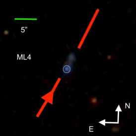
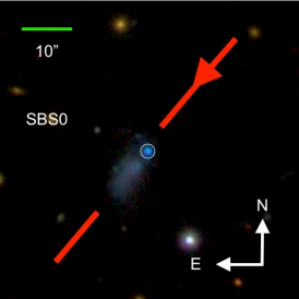
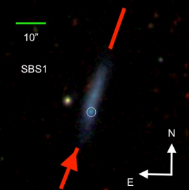
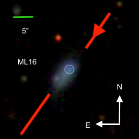
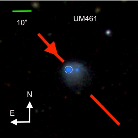
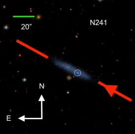
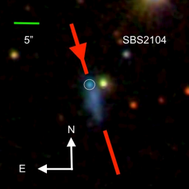
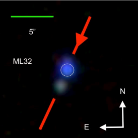
Figure 1.— SDSS color images of the galaxies observed in the paper, with the red bar indicating the position of the spectrograph slit, and the arrow pointing towards the sense of growing distance along the major axis. The green bar provides the scale on the sky. The circles enclose the main star-forming region in each galaxy.

The slit width was selected to be 1 arcsec, according to the seeing at the telescope and also matching the value of our previous observation of these galaxies in Paper I. The spectrograph has two arms, the red and the blue arm, each one with its own detector. All galaxies were observed in both arms, except for HS0822, where we only have the red spectrum. A $2\times 2$ binning of the original images was performed to reduce oversampling. After binning, the dispersion turns out to be 0.52 Å pix^-1 for the red arm and 0.46 Å pix^-1 for the blue arm. Similarly, the spatial scale is 0.44 arcsec pix^-1 for the red arm and 0.40 arcsec pix^-1 for the blue arm. The wavelength coverage for the blue arm is 940 Å  centered at H$\beta$ (from 4390 Å to 5330 Å), whereas the read arm covers 1055 Å around H$\alpha$ (from 6035 Å to 7090 Å). The total exposure time per target was approximately two hours (Table 1), divided in snapshots of 20 minutes as a compromise to simultaneously minimize cosmic-ray contamination and readout noise.

Table 1Parameters of the observed XMP galaxies

Our ID	Galaxy name	Obs. Date	Seeing b	$W_{Ui}$ c	$D$ d	Scale d	Exp. Time	$\log{M_{\star}\,^{e}}$
		dd/mm/yyyy	[arcsec]	[km s-1]	[Mpc]	[pc arcsec-1]	[s]	[M⊙]
ML4	J$030331.26-010947.0$	16/08/2012	0.5	38.1 $\pm$ 2.7	125 $\pm$ 9	608	3600	8.33 $\pm$ 0.33
HS0822	J$082555.52+353231.9$	02/02/2013	1.4	37.8 $\pm$ 1.6	9.6 $\pm$ 0.7	47	7200	6.04 $\pm$ 0.03
SBS0	J$094416.59+541134.3$	15/03/2015	0.9	41.1 $\pm$ 3.2	23.1 $\pm$ 1.6	112	4800	7.05 $\pm$ 0.05
SBS1	J$113202.41+572245.2$	15/03/2015	1.2	40.4 $\pm$3.6	22.5 $\pm$ 1.6	109	7200	7.53 $\pm$ 0.48
ML16	J$114506.26+501802.4$	15/03/2015	1.0	40.1 $\pm$ 4.0	23.6 $\pm$ 1.7	114	7200	6.71 $\pm$ 0.07
UM461	J$115133.34-022221.9$	15/03/2015	1.2	40.6 $\pm$ 4.0	12.6 $\pm$ 0.9	61	6400	6.7 $\pm$ 1
N241a	J$144412.89+423743.6$	15/03/2015	1.0	40.3 $\pm$ 4.0	10.2 $\pm$ 0.7	49	6000	6.52 $\pm$ 0.07
SBS2104	J$210455.31-003522.3$	16/08/2012	0.5	39.0 $\pm$ 2.2	20.1 $\pm$ 1.7	97	7200	6.19 $\pm$ 0.05
ML32	J$230209.98+004939.0$	16/08/2012	0.5	42 $\pm$ 5	138 $\pm$ 10	666	7200	8.39 $\pm$ 0.33

a Target not included in Paper I.
b Mean value of the seeing parameter during the observation of each object, measured by RoboDIMM@WHT
(http://catserver.ing.iac.es/robodimm/).
c Mean FWHM of the telluric lines measured in each spectrum.
d Distance and scale at the position of the source, from NED (NASA/IPAC Extragalactic Database).
e Total stellar mass of the galaxy from MPA-JHU (see Paper I).

The spectral resolution was measured from the FWHM (full width at half maximum) of several telluric lines, using the calibrated data described in the next section. They yield a value of approximately 40 km s^-1 (Table 1), which renders a spectral resolution close to 7500 at H$\alpha$. This resolution is in good agreement with the value expected for the 1 arcsec slit, once the anamorphic magnification of ISIS is taken into account (Schweizer 1979).

The angular resolution during observations ranges from fair (1.3 arcsec) to good (0.5 arcsec), as measured by the seeing monitor at the telescope (Table 1). Additional information on the galaxies and the observations is included in Table 1.

2.2. Data reduction

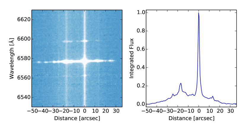
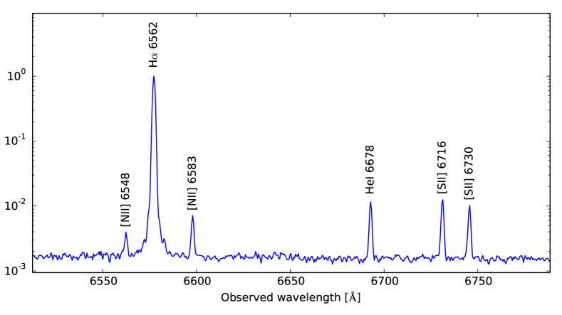
Figure 2.— Reduced spectrum of the galaxy N241, shown as an example. Top left: 2D representation of the spectrum with the observed wavelength in the vertical axis and the spatial position in the horizontal axis. The three emission lines that appear in the image are H$\alpha$ and the [NII] doublet. Top right: wavelength-integrated flux normalized to the maximum value. The peak emission traces the the brightest clump in the galaxy, and it defines the origin of the spatial scale. Bottom: spectrum at the brightest clump, in logarithmic units and normalized to the peak H$\alpha$ emission. The main spectral lines used in the paper are labeled.

The spectra were reduced using standard routines included in the IRAF package. The process comprises bias subtraction, flat-field correction using both dome and sky flat-fields, removal of cosmic-rays (van Dokkum 2001), and wavelength calibration using spectral lamps. In order to evaluate the precision of the wavelength calibration, we measured the variation of the centroids of several sky emission lines along the spatial direction (if the calibration were error-free, the telluric line wavelength should not vary). For different galaxies and emission lines, the root mean square (RMS) variation of the centroids ranges from 0.036 Å to 0.072 Å, which corresponds to 1.6 km s^-1 and 3.3 km s^-1, respectively. It drops even further if only strong telluric lines are considered.

The sky subtraction, the geometrical distortion correction, and the combination of the spectra of each single source were carried out using Python custom-made routines. For the sky subtraction, we performed a linear fit, sampling the sky on both sides of the galaxy spectrum. This model sky emission was then subtracted from each wavelength pixel. The effect of the geometrical distortion is that the spatial and wavelength direction are not exactly perpendicular on the detector. We determine the angle between the two directions as the angle between the continuum emission of the brightest point in the galaxy and the telluric lines. A linear fit allowed us to model the geometric transformation needed to make the spatial and wavelength axes perpendicular. The spectra from different exposures of the same galaxy were re-aligned before combining them. The left panel in Fig. 2 illustrates the final result of the reduction procedure. It contains the spectrum around H$\alpha$ of the galaxy N241. The signal-to-noise ratio (S/N) in continuum pixels has an average value of approximately 5 in the inner 10 arcsec around the brightest Hii region of the galaxy. The S/N in H$\alpha$ ranges from 200 to 900 at the brightest point in the galaxy, decreasing toward the outskirts. Because our main goal is the kinematic analysis, we only performed a rough flux calibration by comparison with the calibrated Sloan Digital Sky Survey spectra of the galaxies (SDSS DR-12; Alam et al. 2015), re-scaling the flux by accounting for the difference between our 1 arcsec slit and the 3 arcsec diameter of the SDSS fiber. Specifically, the flux integrated over the central 3 arcsec of the galaxies is scaled to be equal to 0.42 times the SDSS flux, where 0.42 is the ratio between the areas covered by the slit and the fiber. SDSS spectra of SBS1 and UM461 are not available. Therefore, we use for calibration the spectra of these galaxies analyzed in Paper I.

Since the photometric calibration is only approximate, we have preferred not to correct the spectra for internal reddening in the HII region. This correction is based on comparing the observed Balmer decrement with its theoretical value (e.g., Emerson 1996), which in practice implies comparing fluxes of spectra taken with the red arm (H$\alpha$) and the blue arm (H$\beta$) of the spectrograph. Rather than carrying out an uncertain correction, we have preferred to neglect the small expected reddening (e.g., Sánchez Almeida et al. 2016). If one uses the SDSS spectra of our targets to estimate the Balmer decrement, the ensuing reddening correction implies increasing H$\alpha$ by 50 % or less. Neglecting this correction does not modify any of the conclusions drawn in the paper.

3. Equations used to determine physical parameters

3.1. Parameters from the main H$\alpha$ emission

Mean velocities, velocity dispersions, and rotation curves of the emitting gas are estimated following Sánchez Almeida et al. (2013, Sect. 3), and we refer to this work for details. For the sake of completeness, however, the main assumptions and the resulting equations are provided in the following.

The velocity, $U$, was calculated from the global wavelength displacement of the H$\alpha$ emission. It was derived from the centroid of the line, and also from the central wavelength of a Gaussian fitted to the emission line. Both values generally agree with differences $<1$ km s^-1 in the regions of interest. The error in velocity was estimated assuming the RMS of the continuum variations to be given by noise, and then propagating this noise into the estimated parameter (e.g., Martin 1971). In the case of the centroid, the expression is analytic. For the Gaussian fit, it is the standard error given by the covariance matrix of the fit (e.g., Press et al. 1986, chapter 14). The spatially unresolved velocity dispersion, $W_{U}$, was calculated from the width of the Gaussian model fitted to the line, but also directly from the line profile. We correct the observed FWHM, $W_{U0}$, for the instrumental spectral resolution, $W_{Ui}$ ($\simeq$ 40 km s^-1; see Sect. 2.1 and Table 1), for thermal motions, $W_{Ut}$ ($\simeq$ 25 km s^-1, corresponding to H atoms at $1.5\times 10^{4}$ K, a temperature typical of the HII regions in our galaxies; see Table 2), and for the natural width of H$\alpha$, $W_{Un}$ ($\simeq 7$ km s^-1), so that

$$W_{U}^{2}=W_{U0}^{2}-W_{Ui}^{2}-W_{Ut}^{2}-W_{Un}^{2}.$$ (1)

Table 2Physical parameters for the main star-forming region in the galaxies

ID	HII size	$\pounds_{H\alpha}$	SFR	$\langle 12+\log({\rm O/H})\rangle\,^{a}$	$\langle T_{e}\rangle\,^{a}$	$\langle n_{e}\rangle\,^{b}$	R${}_{e}\,^{c}$	W${}_{U}\,^{d}$	$\log{M_{\mathrm{dyn,turb}}}\,^{e}$
	[arcsec]	[$10^{38}$ erg s-1]	[M⊙ yr-1]		[$10^{4}$ K]	[cm-3]	[kpc]	[km s-1]	[M⊙]
ML4	1.4	30 $\pm$ 4	0.016 $\pm$ 0.002	7.76 $\pm$ 0.06	1.57	13	0.435 $\pm$ 0.012	62 $\pm$ 2	8.3 $\pm$ 0.03
HS0822	1.1	1.9 $\pm$ 0.3	0.00101 $\pm$ 0.00015	7.69 $\pm$ 0.07	1.56	38	0.027 $\pm$ 0.006	36 $\pm$ 2	6.61 $\pm$ 0.1
SBS0	1.0	7.1 $\pm$ 1	0.0038 $\pm$ 0.0005	7.63 $\pm$ 0.06	1.67	129	0.052 $\pm$ 0.011	38 $\pm$ 3	6.95 $\pm$ 0.12
SBS1	1.1	2.3 $\pm$ 0.3	0.00121$\pm$ 0.00017	7.61 $\pm$ 0.09	1.44	84	0.059 $\pm$ 0.018	51 $\pm$ 3	7.27 $\pm$ 0.14
ML16	2.4	7.5 $\pm$ 1.1	0.004 $\pm$ 0.0006	7.92 $\pm$ 0.04	1.46	48	0.139 $\pm$ 0.005	35 $\pm$ 5	7.3 $\pm$ 0.12
UM461	1.2	1.32 $\pm$ 0.19	0.00071 $\pm$ 0.0001	7.38 $\pm$ 0.09	2.47	212	0.036 $\pm$ 0.009	42 $\pm$ 4	6.88 $\pm$ 0.14
N241	1.4	87 $\pm$ 13	0.047 $\pm$ 0.007	7.11 $\pm$ 0.28 f	1.5 g	73	0.035 $\pm$ 0.003	48 $\pm$ 3	6.99 $\pm$ 0.07
SBS2104	1.4	4.1 $\pm$ 0.7	0.0022 $\pm$ 0.0004	7.48 $\pm$ 0.08	1.58	113	0.069 $\pm$ 0.002	18 $\pm$ 5	6.4 $\pm$ 0.2
ML32	1.3	190 $\pm$ 30	0.103 $\pm$ 0.015	7.7 $\pm$ 0.05	1.68	13	0.434 $\pm$ 0.013	55 $\pm$ 4	8.19 $\pm$ 0.06

a Mean value taken from Paper I.

b Inferred from the ratio between [SII]$\lambda$6716 and [SII]$\lambda$6731 (e.g., Osterbrock 1974).

c Half-light radius of the clump, measured from the FWHM of the H$\alpha$ flux distribution.

d Velocity dispersion of the clump, calculated from the H$\alpha$ line of the clump-integrated spectra.

e Dynamical mass of the clump from Eq. (5). Errors do not include the uncertainty in the thermal motion subtraction.

f From Sánchez Almeida et al. (2016).

g Assumed to be similar to the value in the other objects.

The velocity at each spatial pixel along the major axis of the galaxy was fitted with the universal rotation curve by Salucci et al. (2007), i.e.,

$$U(d)=U_{0}+U_{1}\frac{d-d_{0}}{\sqrt{\Delta^{2}+(d-d_{0})^{2}}},$$ (2)

where $U(d)$ stands for the observed velocity at a distance d, $U_{0}$ represents the systemic velocity, i.e., the velocity at the dynamic center $d=d_{0}$, $\Delta$ gives a spatial scale for the central gradient of the rotation curve and, finally, $U_{1}$ provides the amplitude of the rotational velocity.

The dynamical mass enclosed within a distance $d$, $M(d)$, follows from the balance between the centrifugal force and the gravitational pull, and it is given by,

$$M(d)\,\sin^{2}i=(2.33\times 10^{5}\,{\rm M}_{\odot})\,(d-d_{0})\,U^{2}(d),$$ (3)

where $i$ stands for the inclination of the disk along the line-of-sight, and where distances are in kpc, and velocities in km s^-1. The velocity $U$ in Eq. (3) should be the component along the line-of-sight of the circular velocity, $v_{c}\,\sin i$. In the case of a purely stellar system, $U/\sin i$ and $v_{c}$ differ because the stellar orbits are not circular, with the difference given by the so-called asymmetric drift (e.g., Hinz et al. 2001; Binney & Tremaine 2008). In our case, where we measure the velocity of the gas, they also differ because gas pressure gradients partly balance the gravitational force, and this hydro-dynamical force has to be taken into account in the mechanical balance (e.g., Dalcanton & Stilp 2010). In a first approximation (e.g., Dalcanton & Stilp 2010; Read et al. 2016),

$$v_{c}^{2}\simeq U^{2}/\sin^{2}i+0.06\,W_{U}^{2}\,(d-d_{0})/R_{\star},$$ (4)

where the coefficient that gives the correction has been inferred assuming the gas density to drop exponentially with the distance to the center ($|d-d_{0}|$), with a length scale around three times the length scale of the stellar disks $R_{\star}$. This difference between the gaseous and the stellar disk is typical of XMPs (Filho et al. 2013). Since $|d-d_{0}|\sim R_{\star}$, Eq. (4) predicts that even for a large turbulent velocity ($W_{U}\simeq U/\sin i$), the difference between $v_{c}$ and $U/\sin i$ is small. Since we do not know the inclination angle of the galaxies, we cannot apply the correction for pressure gradients in Eq. (4). Thus, we employ $U$ in Eq. (3), knowing that the resulting dynamical masses slightly underestimate the true masses in an amount given by $W_{U}/\sin i$ and Eq. (4).

Our targets have distinct star-forming regions (see Fig. 1), also denoted here as star-forming clumps or starbursts. We refer to the brightest clump in each galaxy as the main star-forming region, to be distinguished from other fainter clumps that appear in some galaxies. They have been highlighted in Fig. 1. The dynamical masses of the individual star-forming clumps are calculated from the velocity dispersion, assuming virial equilibrium,

$$M_{\rm dyn,turb}=(1.20\times 10^{5}\,{\rm M}_{\odot})\,\ R_{e}\,{W_{U}}^{2}.$$ (5)

The half-light radius, $R_{e}$, is calculated as in Paper I, from the FWHM of a 1D Gaussian fitted to the H$\alpha$ flux of the star-forming clump, which is subsequently corrected for seeing (Table 1). $W_{U}$ in Eq. (5) is calculated from the H$\alpha$ line resulting from integrating all the spectra along the spatial axis, from $-R_{e}$ to $+R_{e}$, with the interval centered at the clump. $R_{e}$ in Eq. (5) is given in kpc, and $W_{U}$ in km s^-1. The use of $W_{U}$ to estimate dynamical masses implies excluding thermal motions in the virial equilibrium equation (Eq. [1]). This approximation may be more or less appropriate depending on the structure of the velocity field in the emitting gas. In practice, however, thermal motions are always smaller than $W_{U}$, so that including them does not significantly modify the masses estimated through Eq. (5).

Our long-slit spectra only provide cuts across the star-forming regions. In order to obtain the total luminosity, $\pounds_{\rm H\alpha}$, we assume the region to be circular, with a radius $R_{e}$. Then the flux obtained by integrating the observed spectra from $-R_{e}$ to $+R_{e}$, $F_{\rm H\alpha}$, is corrected according to the ratio between the observed area, $2\,R_{e}\times 1~{}{\rm arcsec}$, and the circular area, $\pi\,R_{e}^{2}$, which renders

$$\pounds_{\rm H\alpha}=2\pi^{2}\,D^{2}\,{{R_{e}}\over{1~{}\rm arcsec}}\,F_{\rm H\alpha},$$ (6)

with $D$ the distance to the source. We take $D$ from NED, as listed in Table 1. SFRs are inferred from $\pounds_{\rm H\alpha}$ using the prescription by Kennicutt & Evans (2012) given in Eq. (20).

3.2. Characterization of the secondary components in the wings of H$\alpha$

When the S/N is sufficiently good, the observed H$\alpha$ profiles show faint broad emission, often in the form of multiple pairs of separate emission-line components (see Fig. 3).

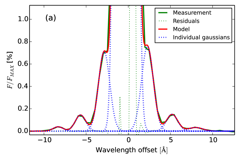
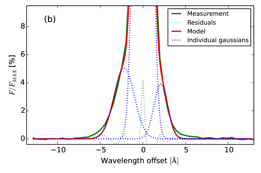
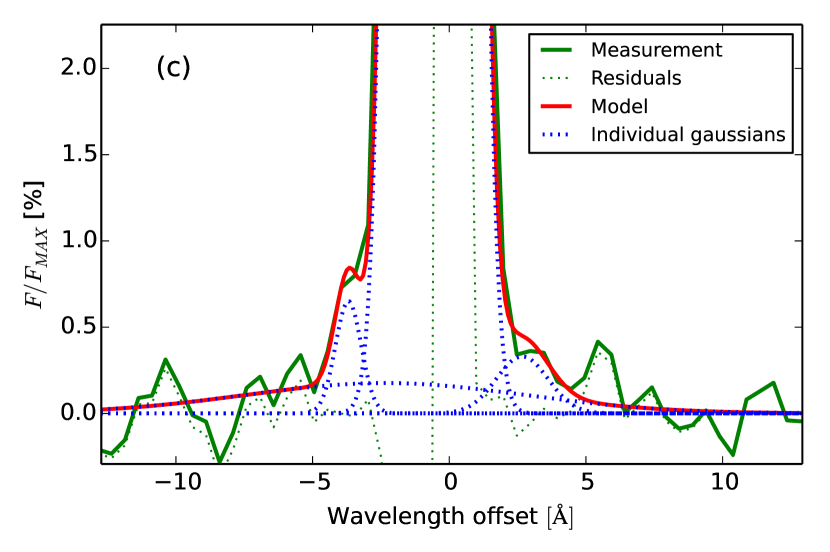
Figure 3.— H$\alpha$ line with the central component saturated to be able to distinguish the secondary components. (a) H$\alpha$ line at the bright core of the galaxy UM461. The observed spectrum (the green solid line) clearly shows seven components: the central one plus three pairs. Our fit reproduces the observation very well (the red solid line) as a superposition of Gaussian functions of various amplitudes, widths, and shifts (the blue dotted lines). The residuals of the fit are also included as the green dotted line. (b) H$\alpha$ at the bright core of the galaxy SBS1, where the components are not very well separated in wavelength. (c) H$\alpha$ at a bright spot of N241, which portrays a case where the S/N is poor compared to the previous cases. The wavelengths are referred to the centroid of the main component, and the fluxes are given in % relative to the maximum flux of the H$\alpha$ profile. Each spectrum corresponds to a single spatial pixel.

The existence of pairs of components is particularly interesting from a physical standpoint, since they may reveal the feedback of star formation on the surrounding medium, or the presence of a black hole (BH; to be discussed in Sect. 5.2).

In order to determine the properties of the secondary lobes (number, wavelength shifts, relative fluxes, etc.), we performed a multi-Gaussian fit to H$\alpha$ using the Python package LMFIT (Newville et al. 2014). The fitting is not unique unless the free parameters are constrained, which we do by attempting to reproduce H$\alpha$ in the brightest pixel of the galaxy as a collection of discrete components, with widths similar to that of the central component. The procedure is detailed below. Several examples of the fit in various S/N conditions are given in Fig. 3. We initialize the fit in the spatial pixel with highest S/N in continuum, where the secondary components clearly stand out. This pixel corresponds to the brightest star-forming region of the galaxy (the bright blue knots in Fig. 1). Then the rest of the pixels are fitted, using as starting values the free parameters obtained in the fit to the adjacent pixel. The number of secondary components is set at the central brightest pixel, where the S/N needed to detect them is highest, and we fix this number for each galaxy. In order to follow each component across the spatial direction, we put two constraints on their spatial variation, namely, (1) the center does not deviate from the previous value by more than twice the wavelength sampling ($\sim 1\,$Å), and (2) the velocity dispersion is bound between a minimum set by the spectral resolution, and twice the value in the previous pixel. These constraints implement the fact that neighbouring pixels are not independent, since our sampling grants at least two pixels per spatial resolution element. As a sanity check, we verified that the constraint on the center of the components does not affect the inferred velocities. The maximum wavelength displacement between two adjacent pixels for all secondary components in the clumps is approximately half the wavelength sampling. Although the S/N decreases with the distance to the brightest pixel, we checked that each detected secondary component has signal at least twice the noise in continuum in all the spectra used to characterize the star-forming regions.

The uncertainties in each parameter can be derived from the covariance matrix of the fit (e.g., Press et al. 1986). However, when the fitted parameters are near the values set by the constraints, the covariance matrix cannot be computed and the uncertainties provided by the Python routine turn out to be unreliable. Therefore, errors are estimated running a MonteCarlo simulation. The best fit profile is contaminated with random noise having the observed S/N. This simulated observation is processed as a true observation, and the exercise is repeated 80 times with independent realizations of the noise. The RMS fluctuations of the parameters thus derived are quoted as 1-sigma errors.

3.3. Mass loss rates

In order to estimate the mass, the mass loss rate, and the kinetic energy corresponding to the secondary components observed in the wings of H$\alpha$ (Fig. 3), we follow a procedure similar to that described in Carniani et al. (2015). It is detailed here both for completeness, and to tune the approach to our specific needs.

We assume that the small emission-line components in the wings of the main H$\alpha$ profile are produced by the recombination of H. Then the luminosity in H$\alpha$, $L_{\rm H\alpha}$, is given by,

$$L_{\rm H\alpha}=\int\,f\,n_{e}\,n_{p}\,j_{\rm H\alpha}\,dV,$$ (7)

where the integral extends to all the emitting volume, and $n_{e}$, $n_{p}$, and $j_{\rm H\alpha}$ represent the number density of electrons and protons, and the emission coefficient, respectively. The symbol $f$ stands for a local filling factor that accounts for a clumpy medium, so that only a fraction $f$ is contributing to the emission. In a tenuous plasma, the emission coefficient is given by (Osterbrock 1974; Lang 1999),

$$j_{\rm H\alpha}\simeq 3.56\times 10^{-25}\,t_{4}^{-1}~{}~{}{\rm erg\,cm^{3}\,s^{-1}},$$ (8)

where $t_{4}$ is the temperature in units of $10^{4}\,$K. The mass of emitting gas turns out to be,

$$M_{g}=\int\,f\,m_{\rm H}\,n_{\rm H}\,X^{-1}\,dV,$$ (9)

where $n_{\rm H}$ is number density of H (neutral and ionized), $m_{\rm H}$ stands for the atomic mass unit, and $X$ is the fraction of gas mass in H. If the gas is fully ionized ($n_{\rm H}=n_{p}$), and the electron temperature and the H mass fraction are constant, then Eqs. (7), (8) and (9) render,

$$M_{g}={{m_{\rm H}\,L_{\rm H\alpha}}\over{X\,j_{\rm H\alpha}\,\langle n_{e}\rangle}_{1}},$$ (10)

with the mean electron density defined as,

$$\langle n_{e}\rangle_{1}={{\int\,f\,n_{p}\,n_{e}\,dV}\over{\int\,f\,n_{p}\,dV}}.$$ (11)

Using astronomical units, and assuming $X=0.75$ (which corresponds to the solar composition; e.g., Asplund et al. 2009), Eq. (10) can be written as

$$M_{g}=3.15\times 10^{3}\,{\rm M}_{\odot}~{}t_{4}\,{{L_{\rm H\alpha}/10^{38}\,{\rm erg\,s^{-1}}}\over{\langle n_{e}\rangle_{1}/10^{2}\,{\rm cm^{-3}}}}.$$ (12)

Assume that the motions associated with the weak emission-line components in the wings of the main profile trace some sort of expansion. The mass loss rate, $\dot{M}_{g}$, is defined as the total mass carried away per unit time by these motions. It can be computed as the flux of mass across a closed surface around the center of expansion,

$$\dot{M}_{g}=\int\,f\,\rho_{g}\,{\bf v\cdot d\Sigma},$$ (13)

where $\rho_{g}$ is the gas density at the surface and ${\bf v}$ represents the velocity of the flow. Assuming that motions are radial, and that the density and filling factor are constant at the surface, the previous integral can be simplified considering a spherical surface of radius $R$,

$$\dot{M}_{g}=4\pi\,R^{2}\,f\,\rho_{g}v_{\rm out},$$ (14)

with the radial speed $v_{\rm out}=|{\bf v}|$. If the moving mass forms a shell of width $\Delta R$ (Fig. 4), then $M_{g}=4\pi\,R^{2}\,f\rho_{g}\,\Delta R$, so that the mass loss rate turns out to be

$$\dot{M}_{g}\simeq M_{g}\,v_{\rm out}\,\Delta R^{-1}.$$ (15)

If the moving mass is distributed on a sphere, then $M_{g}=4\pi\,R^{3}\,f\rho_{g}/3$, and the mass loss rate is still given by Eq. (15) provided that $\Delta R/R\simeq 1/3$. In other words, by using $\Delta R/R\simeq 0.3$ in Eq. (15) one approximately considers the full range of geometries between shells and spheres (for further discussion on the assumptions made to estimate $\dot{M}_{g}$ see, e.g., Maiolino et al. 2012; Keller et al. 2014; or Carniani et al. 2015).

Once the expanding shell geometry has been assumed, the radius of the shell is set by the gas mass and the electron density, since Eq. (9) can be written as,

$$M_{g}\simeq{{8\pi\,m_{H}}\over{1+X}}\,\langle n_{e}\rangle_{2}\,\langle f\rangle_{3}\,R^{2}\,\Delta R,$$ (16)

with the mean values given by

$$\langle n_{e}\rangle_{2}={{\int\,f\,n_{e}\,dV}\over{\int\,f\,dV}},$$

$$\langle f\rangle_{3}={{\int\,f\,dV}\over{\int\,dV}}.$$

Equation (16) assumes the gas to be composed of fully ionized H and He, so that

$$n_{e}\simeq n_{\rm H}+2n_{\rm He}\simeq n_{\rm H}{{1+X}\over{2X}},$$ (17)

which is a reasonable estimate considering that we are dealing with metal-poor gas, such that the metals do not contribute to the electron density. Equation (16) provides a way to estimate the size of the emitting region in terms of the electron density, the filling factor, and the relative width of the shell, explicitly,

$$\Big{[}{{R}\over{14.7~{}{\rm pc}}}\Big{]}^{3}=\Big{[}{{M_{g}}\over{10^{4}\,{\rm M}_{\odot}}}\Big{]}\Big{[}{{\langle n_{e}\rangle_{2}}\over{10^{2}\,{\rm cm}^{-3}}}{{\langle f\rangle_{3}}\over{0.3}}{{\Delta R/R}\over{0.3}}\Big{]}^{-1}.$$ (18)

Figure 4.— Schematic of the geometry used to estimate mass loss rates. The gas is represented in red as clumps which do not fill the full space. The schematic includes the characteristic length-scales, size ($R$) and width ($\Delta R$), and expansion velocity ($v_{\rm out}$). The blue dot points out the center of expansion.

The expansion velocity and the radius allow us to estimate the age of the expanding shell, or the time-lag from blowout,

$$Age=R/v_{\rm out},$$ (19)

where $v_{\rm out}$ is assumed to be constant in time. Since the expansion decelerates, $Age$ in Eq. (19) represents an upper limit to the true age.

A convenient (and intuitive) way of expressing the mass loss rate in Eq. (15) is re-writing the expression in terms of the Star Formation Rate (SFR) estimated using the prescription by Kennicutt & Evans (2012),

$${{\rm SFR}\over{\rm 1M_{\odot}yr^{-1}}}\simeq{{\pounds_{\rm H\alpha}}\over{1.86\times 10^{41}\,{\rm erg\,s^{-1}}}},$$ (20)

which depends only on the total H$\alpha$ flux of the region, $\pounds_{\rm H\alpha}$. We parameterize the H$\alpha$ flux in a weak emission-line component, $L_{\rm H\alpha}$, in terms of total H$\alpha$ flux,

$$L_{\rm H\alpha}=\varepsilon\pounds_{\rm H\alpha},$$ (21)

with $\varepsilon$ the scaling factor inferred from the fits described in Sect. 3.2. We do not correct $\pounds_{\rm H\alpha}$ for extinction in Eq. (20) because the photometric calibration needed to infer it from the Balmer decrement is uncertain (Sect. 2.2), because the main H$\alpha$ lobe and the weak emission components do not necessarily have the same extinction, and because the expected extinction is very low (reddening coefficient around 0.1; Sánchez Almeida et al. 2016). Using Eqs. (20) and (21), Eq. (15) can be expressed as

$${{\dot{M}_{g}}\over{\rm SFR}}\simeq 0.20{{\varepsilon}\over{10^{-3}}}{{v_{\rm out}}\over{10^{2}\,{\rm km\,s^{-1}}}}\,t_{4}\,\Big{[}{{\Delta R}\over{3\,{\rm pc}}}\,{{\langle n_{e}\rangle_{1}}\over{10^{2}\,{\rm cm^{-3}}}}\Big{]}^{-1}.$$ (22)

Another important parameter derived from the gas mass and velocity is the kinetic energy involved in the outflow,

$$E_{k}={{1}\over{2}}M_{g}\,v_{\rm out}^{2}\simeq 10^{51}\,{\rm erg}\,{{M_{g}}\over{10^{4}\,{\rm M_{\odot}}}}\,\Big{[}{{v_{\rm out}}\over{10^{2}\,{\rm km\,s^{-1}}}}\Big{]}^{2}.$$ (23)

The equation has been written in units of $10^{51}{\rm erg}$, which is the typical kinetic energy released in a core-collapse supernova (SN; e.g., Leitherer et al. 1999; Kasen & Woosley 2009), corresponding to the explosion of a massive star.

This energy range is also within reach of accreting BH of intermediate mass, like the direct collapse $10^{5}~{}{\rm M}_{\odot}$ BH seeds needed to explain the existence of super-massive BHs in the early Universe (e.g., Volonteri 2010; Ferrara et al. 2014; Pacucci et al. 2016). Assuming that the BH releases kinetic energy at a fraction of the Eddington limit, $\psi$, and that the accretion event has a duration, $\Upsilon$, then

$$E_{BH}\simeq 10^{51}\,{\rm erg}\,{{\psi}\over{0.1}}\,{{\Upsilon}\over{25~{}{\rm yr}}}\,{{M_{BH}}\over{10^{5}\,{\rm M}_{\odot}}},$$ (24)

with $M_{BH}$ the BH mass (e.g., Frank et al. 2002).

3.4. Mass of the central object

In principle, the observed faint emission-line pairs in the wings of H$\alpha$ might also be generated in a rotating disk around a massive object (e.g., Epstein 1964). Then the approximation used to estimate the radius of the shell in Eq. (18) still holds, except that

$$\Big{[}{{R}\over{27.6~{}{\rm pc}}}\Big{]}^{3}=\Big{[}{{M_{g}}\over{10^{4}\,{\rm M}_{\odot}}}\Big{]}\Big{[}{{\langle n_{e}\rangle_{2}}\over{10^{2}\,{\rm cm}^{-3}}}{{\langle f\rangle_{3}}\over{0.3}}{{\Delta R/R}\over{0.3}}{{\Delta z/R}\over{0.3}}\Big{]}^{-1},$$ (25)

where $\Delta R$ represents the difference between the inner and outer radii, and $\Delta z$ stands for the thickness of the disk. This size, together with the circular velocity, $v_{c}$, directly inferred from the spectra, allow us to estimate the mass of the central object, $M_{\bullet}$, from the balance between gravity and centrifugal force,

$${M_{\bullet}}\simeq{7.0\times 10^{7}\,{\rm M}_{\odot}}\,{{R}\over{30\,\rm pc}}\,\Big{(}{{v_{c}}\over{10^{2}\,{\rm km\,s^{-1}}}}\Big{)}^{2}.$$ (26)

4. Rotation, turbulent motions, and chemical properties

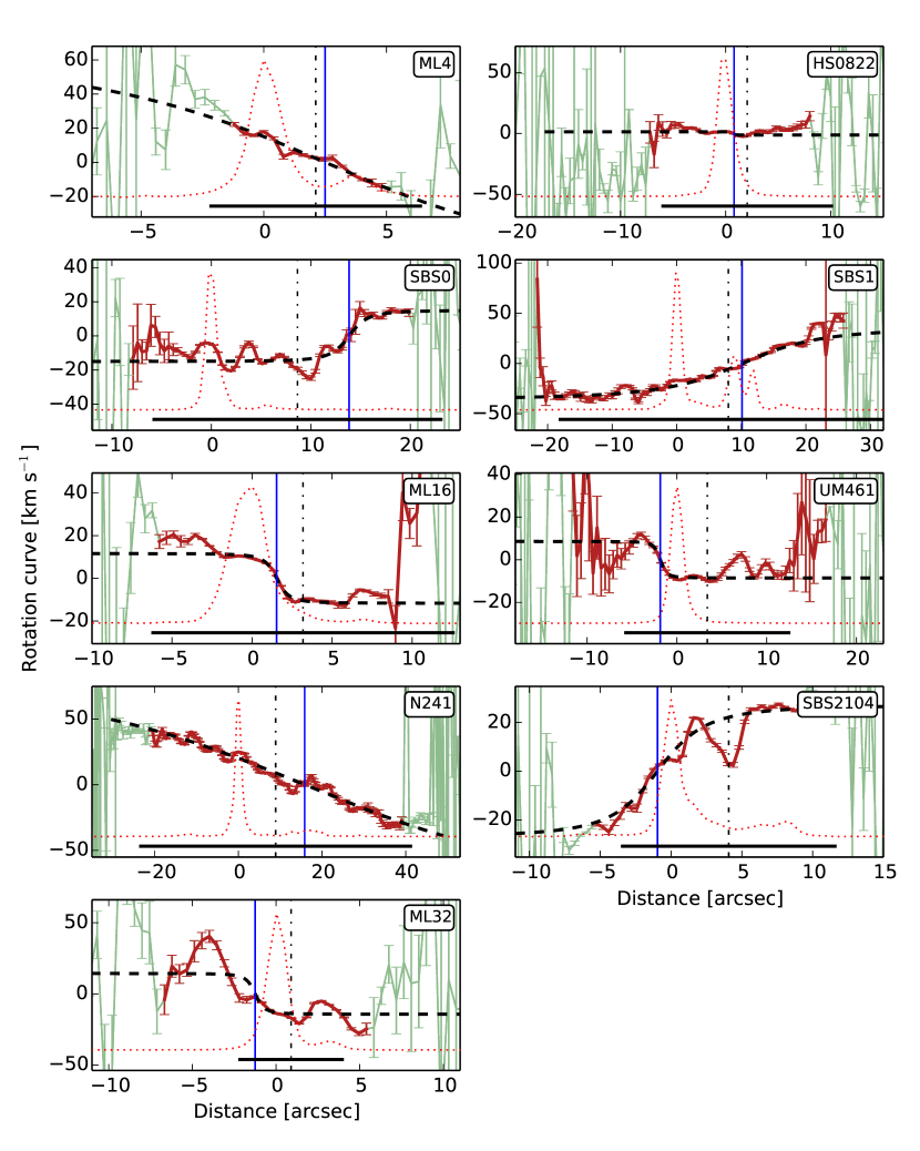
Figure 5.— Rotation curves for the XMPs, i.e., velocity versus position along the slit. The velocities were derived using a Gaussian fit to the H$\alpha$ line profile. The actual observed points show error bars joined by a continuous line, which is either green or red, depending on whether the S/N of the spectra in the continuum is smaller (green) or larger (red) than one. Only the points in red have been used to fit the universal rotation curve, shown as the black dashed line, with the vertical blue line identifying the position of the dynamical center inferred from the fit. The zero of the velocity scale is set by the fit at the dynamical center. The red dotted line represents the H$\alpha$ flux scaled from zero to the maximum value. Distances are referred to the point with largest H$\alpha$ flux. The horizontal solid black line gives the galaxy diameter, inferred from the 25 mag arcsec^-2 isophote, and provided by NED. It is centered in the photometric midpoint marked by the vertical dotted-dashed line.

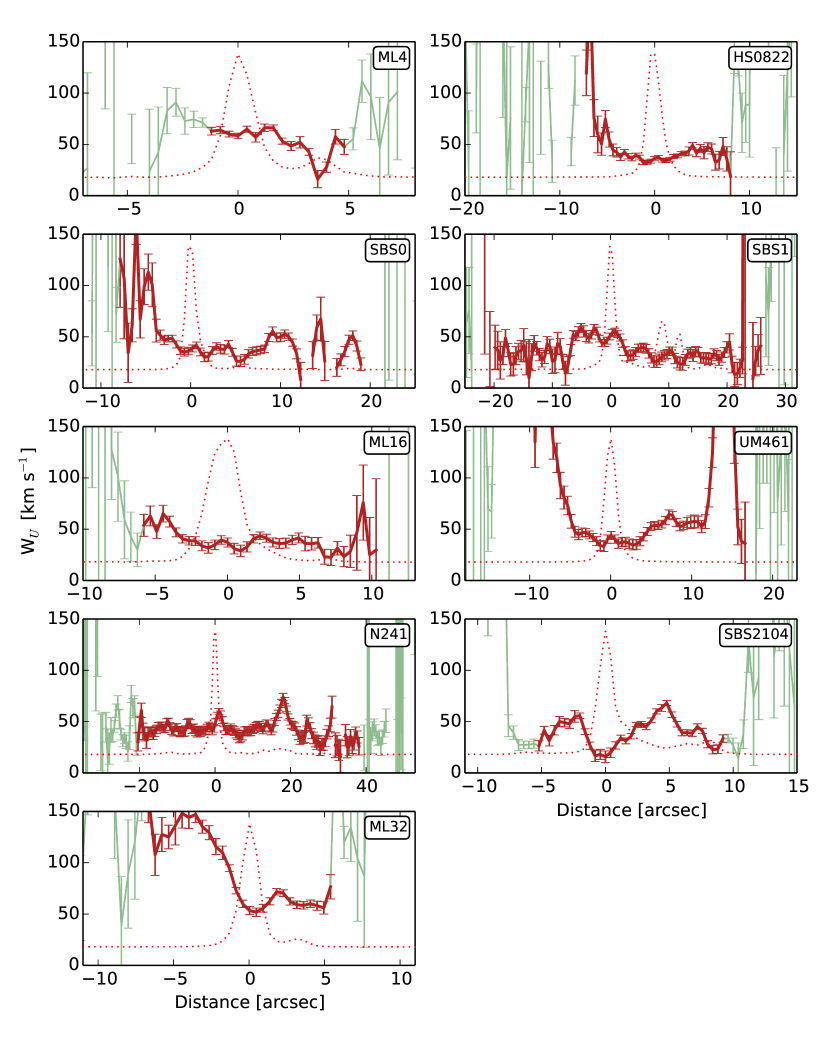
Figure 6.— Similar to Fig. 5 with the FWHM velocity dispersion. The range in abscissas is the same as in Fig. 5.

Figure 5 shows the rotation curve of all the galaxies analyzed in this study. It represents the velocities inferred from the Gaussian fit, but the results are similar when using centroids (Sect. 3.1). Most galaxies seem to rotate, although HS0822 and SBS0 do not. The rotation curve of UM461 may suggest some rotation, but it may also be compatible with the absence of rotation. The difficulty in detecting rotation in UM461 could be due to projection effects; UM461 appears face-on in the SDSS image, with the galaxy showing a rounded faint envelope enclosing its two bright knots (Fig. 1). All rotation curves present small-scale velocity irregularities, often with an amplitude comparable to the velocity gradient across the whole galaxy. The rotation of the galaxies ML4, SBS1, N241 is clear, whereas other galaxies are more affected by these small-scale irregularities. Galaxies SBS2104 and ML32 could host counter-rotating components, like those found in tadpole galaxies by Sánchez Almeida et al. (2013), although, in this case, the center of the counter-rotating structure does not match the main star-forming region. Figure 6 shows the FWHM velocity dispersion inferred from H$\alpha$. Typical values at the position of the main starburst are between 20 and 60 km s^-1 (Table 2). We note that the regions with possible counter-rotating components also show an increase in the velocity dispersion: c.f., Figs. 5 and 6 for SBS2104 ($d\simeq 4$ arcsec) and ML32 ($d\simeq 2$ arcsec).

We fitted the universal rotation curve by Salucci et al. (2007), given in Eq. (2), to the observed velocities. The four free parameters of the non-linear fit ($U_{0}$,$U_{1}$, $d_{0}$, and $\Delta$) were derived using the Python package LMFIT (Newville et al. 2014). The fits are shown as black dashed lines in Fig. 5. The fits are not particularly good, but they allow us to have an idea of the amplitude of the rotation curve and the dynamical center of the galaxies. These properties are summarized in Table 3. Even though the position of the dynamical center is very uncertain (see Fig. 5), they do not seem to overlap with the position of the main star-forming region.

Independently of the properties of the rotation, we do find a recurrent behavior for the velocity and velocity dispersion at the star-forming region. The velocity tends to be constant within the spatial extent of the clump. This is clear in, e.g., SBS2104 and ML16 (see the velocity curves in Fig. 5 at the point where the H$\alpha$ emission peaks). If the spatial resolution of the observations were insufficient to resolve the individual clumps, then one would expect that the velocity, and all the other properties inferred from the shape of the H$\alpha$ line, would be constant within the spatially unresolved clump. However, insufficient spatial resolution is not responsible for the observed behavior for two reasons: (1) many clumps are well resolved; e.g., ML16 has a FWHM of 3 arcsec (Fig. 5) when the seeing was only 1 arcsec FWHM (Table 1), and (2) the velocity dispersion is not constant within the starburst clump (see Fig. 6).

These two properties, i.e., constant velocity with varying velocity dispersion, are clearer in Fig. 7. It shows the H$\alpha$ flux across all the clumps of the individual galaxies (the dotted lines in all the panels). They have been re-scaled in abscissa and ordinate so that all of the H$\alpha$ flux profiles look approximately the same in this representation (we normalize each profile to its maximum flux and to its size). The figure also includes the rotation curve around the star-forming region (bullet symbols and solid lines), once the average velocity in the region has been removed. Note that all rotation curves tend to flatten at the location of the star-forming clump. The velocity is uniform, as if the star-forming region were a kinematically distinct entity. Note also how the velocity dispersion (shown as asterisks joined by solid lines in Fig. 7) varies across the clump. Three patterns for the variation of the velocity dispersion can be distinguished, namely, the velocity dispersion has a local maximum coinciding with the center of the star-forming clump (Fig. 7, top panel; Type 1), the velocity dispersion increases across the clump (Fig. 7, middle panel; Type 2), and the velocity dispersion presents a minimum at the center of the clump (Fig. 7, bottom panel; Type 3).

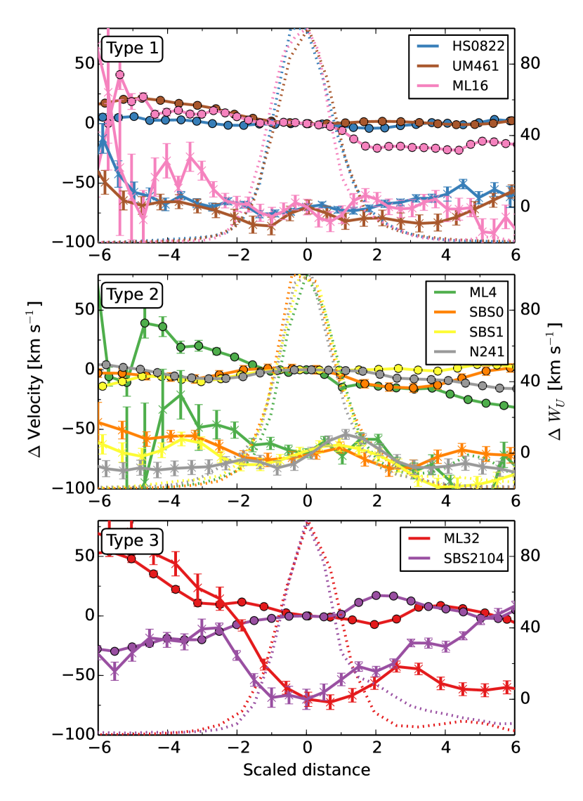
Figure 7.— Variation of the velocity (bullet symbols) and velocity dispersion (asterisks) across the star-forming regions of the XMPs. Distances, in the abscissa axis, are referenced to the position of the star-forming region and normalized to its size. For this reason, the variation of the H$\alpha$ flux across the region, shown as dotted lines, is always centered at distance zero, and always has the same width. The velocity turns out to be constant within the star-forming clump, whereas the velocity dispersion follows three distinct patterns, labelled as Type 1 (shown in the top panel), Type 2 (middle panel), and Type 3 (bottom panel). In Type 1, the dispersion presents a local maximum at the center of the starburst. In Type 2, however, the dispersion increases across the region towards the position that is closest to the galaxy photometric center. The Type 3 pattern presents a minimum at the center of the star-forming region. Different colors refer to different galaxies, as indicated by the insets. The monikers used for the XMPs are in Table 1. The average velocity and velocity dispersion in each star-forming clump have been subtracted from the plots, so that the velocity and velocity dispersion are zero at the clump.

The first case may be qualitatively understood if the star-forming region is undergoing a global expansion. The velocity dispersion peaks in the central part, where the Doppler signal of the approaching and receding parts is largest. In this instance, the velocity remains constant, tracing the rotational velocity at the origin of expansion. The difference between the velocity dispersion at the center and at the sides of the starburst can be used to estimate the expansion velocity of the region. If the difference is of the order of 20 %, and $W_{U}$ is around 40 km s^-1 (see HS0822, UM461, and ML16 in Table 2), then an expansion able to create the observed excess of central velocity dispersion has to be of the order of 13 km s^-1. We have assumed that the turbulent and expansion velocity add up quadratically in their contribution to $W_{U}$. The mass loss rate resulting from the possible global expansion is worked out in Sect. 6.

In the second case (Type 2; Fig. 7), the dispersion always increases towards positive distances which, by construction, point to the photometric center of the galaxies. In other words, it is largest in the part of the star-forming clump that is closest to the galaxy center. As we discussed above, this is not an observational bias due to insufficient spatial resolution. Although we can only speculate at this point, the result is very suggestive. The excess velocity dispersion in the center-side of Types 2 may indicate an intensification of the turbulence of the gas in that particular part of the starburst. Such an increase may indicate the collision of the starburst gas with the ISM of the host galaxy, as if the star-forming regions were inspiraling towards the galaxy center. This migration to the galaxy center is expected from tidal forces acting upon massive gas clumps (see, e.g., Elmegreen et al. 2008; Ceverino et al. 2016; Hinojosa-Goñi et al. 2016); the large starbursts in our XMPs may be going through such a process at this moment.

The Type 3 pattern presents a minimum velocity dispersion, coinciding with the starburst (Fig. 7); it may reflect the past expansion of the region. As an adiabatic contraction increases the turbulence in a contracting medium (e.g., Murray & Chang 2015), an expansion leads to adiabatic cooling and to a drop of the turbulence (e.g., Robertson & Goldreich 2012). A past expansion phase may have produced the observed decrease in velocity dispersion, even if the phase is already over and it does not appear in the form of a Type 1 pattern. The same kind of local minima in velocity dispersion has been observed in young star cluster complexes of nearby galaxies (e.g., Bastian et al. 2006).

We have calculated the dynamical mass that accounts for the velocity dispersion if the clump was in virial equilibrium, as described by Eq. (5). The results are in Table 2. They are similar to the total stellar mass of the galaxy and thus, very large. They are also comparable to the dynamical mass of the galaxy inferred from the rotation curve (Table 3), even though these masses are lower limits because of the (unknown) inclination of the galaxies, and because of the existence of pressure gradients (see the discussion in Sect. 3).

The fact that the star-forming regions have well defined kinematical properties, suggests that they are distinct entities within the host galaxy.

Table 3Properties of the rotation curve

ID	$U_{1}\,^{a}$	$d_{0}\,^{b}$	$\log(M\,\sin^{2}{i})\,^{c}$	$|d_{\mathrm{l}}-d_{0}|\,^{c}$
	[km s-1]	[arcsec]	[M⊙]	[arcsec]
ML4	-70 $\pm$ 200	2 $\pm$ 2	8.4	3.7
HS0822	-1.3 $\pm$ 0.2	0.8 $\pm$ 80	5.2	7.5
SBS0	15 $\pm$ 1.2	13.8 $\pm$ 0.5	8.1	21.7
SBS1	36 $\pm$ 4	10.1 $\pm$ 0.08	9.0	31.7
ML16	-11.7 $\pm$ 0.7	1.53 $\pm$ 0.09	7.4	7.6
UM461	-8.6 $\pm$ 0.7	-1.85 $\pm$ 0.08	7.2	13.4
N241	-90 $\pm$ 50	16 $\pm$ 10	9.0	40.8
SBS2104	27 $\pm$ 8	-1 $\pm$ 0.9	8.2	10.2
ML32	-14 $\pm$ 7	-1.2 $\pm$ 0.4	8.3	6.6

a Amplitude resulting from fitting Eq. (2) to the observed

rotation curve.

b Dynamical center resulting from fitting Eq. (2) to the

observed rotation curve.

c Dynamical mass of the galaxy. Based on Eq. (3), considering

up to the largest distance from $d_{0}$ with sensible velocity

measurements, dl.

4.1. Chemical properties

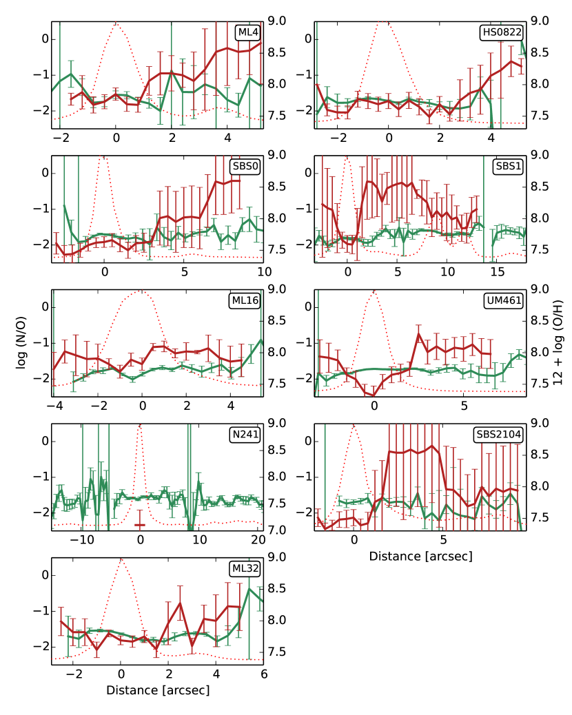
Figure 8.— Variation of the metallicity ($12+\log[{\rm O/H}]$), N/O ratio, and SFR along the major axis of the XMPs. The red solid line is the metallicity of the galaxy from Paper I, except for N241, where a mean value for the clump was obtained from Sánchez Almeida et al. (2016). The green solid line is the variation of the N/O ratio. The red dotted line represents the H$\alpha$ flux scaled to the maximum value at the clump, which is a proxy for the SFR.

A separate, but important, result from the analysis of the spectra deals with the metallicity. Most of the XMPs that we study are characterized by having a drop in gas-phase metallicity associated with the main starburst (Paper I). We searched for possible relationships between such metallicity inhomogeneities and the kinematic properties described above but found no correlation. What we found, however, is a notable lack of correlation between the metallicity (as traced by O/H) and the ratio N/O. It appears in Fig. 8, where the variation of the metallicity, SFR and N/O ratio is displayed. The N/O ratio was estimated from [NII]$\lambda$5583 and [SII]$\lambda$6716,6731 following the calibration by Pérez-Montero & Contini (2009), which is almost independent of dust reddening (it was not estimated in Paper I because of the difficulty in separating [NII] from H$\alpha$, given the limited wavelength resolution of that spectra). Figure 8 shows that the N/O ratio remains fairly constant along the galaxy, even at the position of the main starbursts, where the H$\alpha$ flux peaks and the metallicity drops. The lack of correlation between the ratios N/O and O/H represents the general behavior. This observational fact is consistent with the gas accretion scenario. If the accretion of metal-poor gas is triggering the observed starburst, then the fresh gas would locally reduce the O/H ratio in the star-forming region relative to the rest of the galaxy. However, mixing with external gas cannot modify the pre-existing ratio between metals, leaving the N/O ratio unchanged. This argument has been put forward before to support the gas accretion scenario (Amorín et al. 2010, 2012; Sánchez Almeida et al. 2014a). The value for $\log({\rm N/O})$ that we infer, around $-1.5$, is also consistent with the N/O ratio found in metal-poor $\alpha-$enhanced stars in the solar neighborhood (e.g., Israelian et al. 2004; Spite et al. 2005). Since the star formation is enhanced where the O/H ratio drops, the lack of correlation between the ratios N/O and O/H reveals a lack of correlation between N/O and the SFR. This property seems to be common among star-forming galaxies at all redshifts (e.g., Pérez-Montero et al. 2013), and supports the metal-poor nature of the gas that forms stars.

5. Properties of the multiple components

5.1. Expanding shell interpretation

The first significant result is the mere existence of multiple components in the wings of H$\alpha$, which are often paired, so that for each red component there is a blue component with a similar wavelength shift and amplitude (see the example in Fig. 3a). This fact discards spatially-unresolved, optically-thin, uniform expanding shells as the source of emission in the line wings, since they produce a top-hat line profile without individual emission peaks (e.g., Zuckerman 1987; Cid Fernandes & Terlevich 1994; Tenorio-Tagle et al. 1996, and also Appendix A). However, the two-hump emission can be caused by a non-spherically-symmetric shell, or a shell having internal absorption (the other alternatives are analyzed and discarded in Sect. 5.2). Even though the observed amplitudes are similar, the blue component of each pair tends to be larger than the red component. Figure 9 shows the ratio between the area of the red and the blue components, and in all but one case, this ratio is one or smaller, considering error bars. Moreover, if one of the components is missing, it tends to be the red one. These two facts suggest a dusty expanding shell model, where the receding cap of the shell is obscured by the approaching cap (see Appendix and Fig. 17). These issues are discussed in detail in Sect. 5.2.

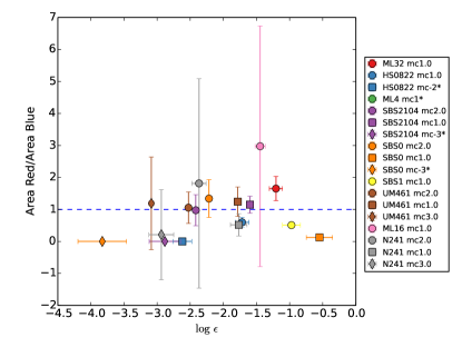
Figure 9.— Area ratio between the blue and red emission of paired components versus mean strength of the secondary components relative to the central component, i.e., area ratio versus $\varepsilon$. Each point corresponds to one pair in one of the galaxies, as indicated in the inset – each galaxy has a color, and the different symbols with same color correspond to different weak components of the same galaxy. When only one component exists, it tends to be the blue one (they are marked with an asterisk in the inset). We show unpaired components as having an area ratio equal to zero. Except for ML32, the ratio is consistent with one or smaller. There is no obvious trend in the observed scatter plot.

The color code employed in Figs. 9 — 15 assigns a color to each galaxy, and then the different symbols of the same color correspond to the various pairs of secondary components in that galaxy.

Using the equations in Sect. 3.3, we have estimated the mass, mass loss rate, and kinetic energy associated with all the weak components in the H$\alpha$ wings (Sect. 3.2; Fig. 3). The mean values, as well as the errors, are given in Table 4.

Table 4Parameters for the weak components in the H$\alpha$ wings ^a

ID b	Velocity c	$\varepsilon\,^{d}$	red/blue e	$M_{g}$	$R$	$\dot{M_{g}}$	$E_{k}$	Age
	[km s-1]			[$10^{3}$ M⊙]	[pc]	[${\rm M}_{\odot}$ yr-1]	[$10^{51}$ erg]	[$10^{4}$ yr]
ML4-1. *	98 $\pm$ 8	0.031 $\pm$ 0.012	—	37 $\pm$ 15	30 $\pm$ 4	0.41 $\pm$ 0.17	3.5 $\pm$ 1.5	30 $\pm$ 5
HS0822-1.0	114 $\pm$ 6	0.019 $\pm$ 0.005	0.6 $\pm$ 0.15	0.47 $\pm$ 0.13	4.9 $\pm$ 0.5	0.037 $\pm$ 0.011	0.061 $\pm$ 0.018	4.2 $\pm$ 0.5
HS0822-2 *	-248 $\pm$ 9	0.0024 $\pm$ 0.0008	—	0.06 $\pm$ 0.02	2.5 $\pm$ 0.3	0.02 $\pm$ 0.008	0.036 $\pm$ 0.013	0.97 $\pm$ 0.12
SBS0-1.0	16 $\pm$ 8	0.28 $\pm$ 0.13	0.12 $\pm$ 0.03	8 $\pm$ 4	8.5 $\pm$ 1.3	0.05 $\pm$ 0.04	0.02123 $\pm$ 0.02	50 $\pm$ 30
SBS0-2.0	211 $\pm$ 0.4	0.0061 $\pm$ 0.0005	1.3 $\pm$ 0.6	0.18 $\pm$ 0.03	2.35 $\pm$ 0.13	0.054 $\pm$ 0.009	0.079 $\pm$ 0.013	1.09 $\pm$ 0.06
SBS0-3 *	-370 $\pm$ 20	0.00015 $\pm$ 0.00013	—	0.004 $\pm$ 0.004	0.68 $\pm$ 0.2	0.008 $\pm$ 0.007	0.006 $\pm$ 0.005	0.18 $\pm$ 0.05
SBS1-1.0	98 $\pm$ 3	0.11 $\pm$ 0.03	0.51 $\pm$ 0.03	1.3 $\pm$ 0.4	5.3 $\pm$ 0.6	0.08 $\pm$ 0.03	0.12 $\pm$ 0.04	5.3 $\pm$ 0.6
ML16-1.0	110 $\pm$ 40	0.036 $\pm$ 0.006	3 $\pm$ 4	2.6 $\pm$ 0.6	8 $\pm$ 0.6	0.12 $\pm$ 0.05	0.3 $\pm$ 0.2	7 $\pm$ 2
UM461-1.0	116 $\pm$ 3	0.0165 $\pm$ 0.002	1.2 $\pm$ 0.5	0.08 $\pm$ 0.015	1.53 $\pm$ 0.09	0.021 $\pm$ 0.004	0.011 $\pm$ 0.002	1.29 $\pm$ 0.09
UM461-2.0	248 $\pm$ 3	0.00297 $\pm$ 7e-05	1.1 $\pm$ 0.5	0.014 $\pm$ 0.002	0.86 $\pm$ 0.04	0.014 $\pm$ 0.002	0.0088 $\pm$ 0.0013	0.34 $\pm$ 0.017
UM461-3.0	372 $\pm$ 4	0.00082 $\pm$ 7e-05	1.2 $\pm$ 1.4	0.0039 $\pm$ 0.0007	0.56 $\pm$ 0.03	0.0089 $\pm$ 0.0016	0.0054 $\pm$ 0.0009	0.148 $\pm$ 0.008
N241-1.0	115 $\pm$ 4	0.017 $\pm$ 0.005	0.5 $\pm$ 0.3	10 $\pm$ 3	10.7 $\pm$ 1.2	0.35 $\pm$ 0.12	1.3 $\pm$ 0.4	9.2 $\pm$ 1
N241-2.0	236 $\pm$ 9	0.0043 $\pm$ 0.0011	2 $\pm$ 3	2.4 $\pm$ 0.7	6.8 $\pm$ 0.6	0.28 $\pm$ 0.09	1.3 $\pm$ 0.4	2.8 $\pm$ 0.3
N241-3.0	395 $\pm$ 7	0.0012 $\pm$ 0.0005	0.2 $\pm$ 1.4	0.6 $\pm$ 0.3	4.4 $\pm$ 0.7	0.2 $\pm$ 0.1	1 $\pm$ 0.5	1.08 $\pm$ 0.17
SBS2104-1.0	112 $\pm$ 2	0.025 $\pm$ 0.002	1.1 $\pm$ 0.3	0.46 $\pm$ 0.09	3.4 $\pm$ 0.2	0.052 $\pm$ 0.01	0.057 $\pm$ 0.011	2.96 $\pm$ 0.19
SBS2104-2.0	246 $\pm$ 4	0.0038 $\pm$ 0.0002	1 $\pm$ 0.5	0.07 $\pm$ 0.013	1.8 $\pm$ 0.11	0.032 $\pm$ 0.006	0.042 $\pm$ 0.008	0.72 $\pm$ 0.04
SBS2104-3 *	-372 $\pm$ 10	0.0013 $\pm$ 0.0007	—	0.024 $\pm$ 0.014	1.3 $\pm$ 0.2	0.024 $\pm$ 0.014	0.033 $\pm$ 0.019	0.33 $\pm$ 0.06
ML32-1.0	93 $\pm$ 9	0.062 $\pm$ 0.014	1.7 $\pm$ 0.4	490 $\pm$ 130	71 $\pm$ 6	2.2 $\pm$ 0.7	42 $\pm$ 14	74 $\pm$ 10

a The error bars in this table represent the standard deviation across the starburst (velocity, $\varepsilon$, and area ratio), or errors for the value obtained

from the mean H$\alpha$ line of the starburst (the rest).

b The number added to the galaxy name identifies each one of the pairs of components in the line profiles, with ‘1.0’ representing the pair of

lowest velocity, ‘2.0’ the second lowest velocity, and so on.

c Velocity of the center of the component. Negative, when there is no red counterpart to the blue component. In paired components, mean of

the absolute value of the pair.

d Area ratio between the secondary component and the main component. In paired components, total $\varepsilon$ of the pair.

e Area ratio between the red and blue emissions in the case of paired components.

$*$ Unpaired component.

The velocities and the ratio between the secondary components and the central component, $\varepsilon$, are provided directly by the multi-Gaussian fit described in Sect. 3.2. In the case of paired components, the velocity is the mean of the absolute value of the two velocities, and $\varepsilon$ is the total $\varepsilon$ of the pair. The estimates also depend on the temperature and electron density of the emitting plasma, as well as on the relative thickness of the shell, $\Delta R/R$, and the filling factor, $f$.

The electron temperature is taken from the data used to determine oxygen abundance in Paper I. Specifically, we use the mean over the main star-forming region of the galaxy. The electron density has been inferred from the ratio of the emission lines [SII]$\lambda$6716 and [SII]$\lambda$6731, following the standard procedure (e.g., Osterbrock 1974), using the mean value over the whole star-forming region. These two lines are present within the spectral range observed with the WHT. Electron densities and temperatures are listed in Table 2. As for the thickness of the shell, we use $\Delta R/R=0.3$ (see Sect. 3.3). The filling factor, $f$, is assumed to be one.

The velocities of the weak secondary components are typically in excess of 100 km s^-1 (see Table 4). These velocities are very large compared with the rotational and turbulent velocities of the galaxies (Sect. 4), and, hence, are almost certainly larger than the escape velocity of the galaxy, expected to be of the order of the rotational plus turbulent velocity in the disk (e.g., Binney & Tremaine 2008). Assuming that the components in the wings correspond to outflows in expanding shells, it is still unclear whether or not the involved mass will finally escape from the galaxy. It all depends on the ISM of the host galaxy, and the pressure it exerts on the expanding shell. The issue is analyzed in Sect. 5.2, with the conclusion that the gas will likely escape. The mass involved in these motions is given in Table 4 and summarized in Fig. 10.

Figure 10.— Mass loss rate versus gas mass for the faint components observed in the wings of H$\alpha$. The color code and symbols have the same meaning as in the previous figure, which is indicated in the inset.

The masses are in the range between $10\,{\rm M}_{\odot}$ and $10^{5}\,{\rm M}_{\odot}$, and they represent a few percent of the total gas mass in the HII region (the parameter $\varepsilon$ in Table 4 gives the flux ratio between the secondary and the main emission lobe, and it has been taken as a proxy for the mass ratio; see Eqs. [21] and [22]). These masses are very small compared to the stellar masses and the dynamical masses of the entire galaxies (Tables 1 and 3).

Figure 10 shows that the mass loss rate scales with the gas mass, since the velocities and radii of the different components and galaxies are similar. The weak components have associated mass loss rates between $10^{-2}$ and 1 M_⊙ yr^-1. They are very significant compared with the SFRs, as is attested in Fig. 11, which shows the mass loading factor, $\dot{M}_{g}/{\rm SFR}$. Most mass loading factors are in excess of one, meaning that for every mass unit transformed into stars, several mass units are swept away. Whether this mass escapes the HII region, and later on, the galaxy, we cannot know from our observations. However, cosmological numerical simulations predict large mass loading factors in low mass galaxies (10 is not uncommon; see, e.g. Peeples & Shankar 2011; Davé et al. 2012; Oppenheimer et al. 2012; Bournaud et al. 2014; Thompson & Krumholz 2016).

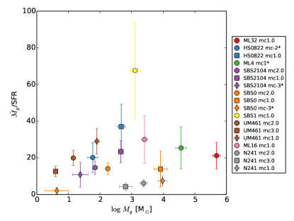
Figure 11.— Mass loading factor ($\dot{M}_{g}/{\rm SFR}$) versus gas mass, for the weak components observed in the wings of H$\alpha$. All factors are larger than one, meaning that for every unit mass transformed in stars, several of units are swept away by the expansion. The color code and symbols have the same meaning as in previous figures, which is indicated in the inset.

Mass loading factors observed in high redshift objects are generally lower than the ones we infer (say, of the order of 2, e.g., Newman et al. 2012; Martin et al. 2012), likely because they refer to massive galaxies ($\log(M_{\star}/M_{\odot})>10$). However, it is not uncommon to find factors up to 10 in local dwarfs (e.g., Martin 1999; Veilleux et al. 2005). A caveat is in order, though. We are assuming the density of the shell to be the same as the mean density of the star-forming region. If the expanding shell builds up mass by sweeping gas around the explosion site, its density is expected to be higher than the mean density of the region. This increase of density would reduce our mass loading factor estimates (see Eq. [22]).

Figure 12 shows the kinetic energy associated with the weak components. As with the mass loss rate, it scales with the mass of gas that is involved in the motion. Figure 12 also shows the energy typically associated with a core-collapse SN explosion, of the order of $10^{51}$ ergs (e.g., Leitherer et al. 1999). The energies involved in the observed motions are usually around this value, albeit smaller; ML32 is the only exception. Therefore, energy-wise, the components may be tracing shells produced by individual SN explosions. ML32 would require some 10 SN exploding simultaneously.

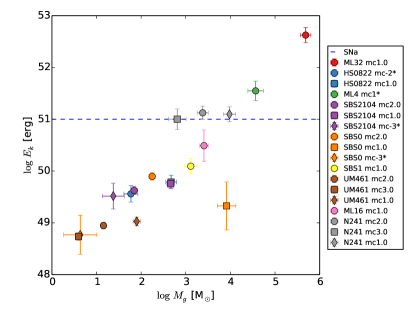
Figure 12.— Kinetic energy versus gas mass, for the weak components observed in the wings of H$\alpha$. The line of $10^{51}$ erg corresponds to the typical kinetic energy released by a core-collapse SN, characteristic of massive stars. The color code and symbols have the same meaning as in previous figures, which is indicated in the inset.

Depending on the IMF (initial mass function), population synthesis models predict a SN rate between 0.02 and 0.005 yr^-1 for a constant SFR=1 M_⊙ yr^-1 (Leitherer et al. 1999). Using a value in between these two extremes, say 0.01 yr^-1/$({\rm M}_{\odot}{\rm yr}^{-1})$, the SFRs of our star-forming regions (Table 2) allow us to estimate the expected SN rates assuming the observed SFRs to be constant. The predicted SN rate turns out to be between $10^{-3}$ and $10^{-5}~{}{\rm yr^{-1}}$, which corresponds to a time-lag between SN explosions ($\tau_{SN}$, defined as the inverse of the SN rate) from 1000 yr to 0.1 Myr. These rates suffice to maintain the observed signals. Figure 13 provides $Age/\tau_{SN}$ for individual shells. $Age>\tau_{SN}$ in half of the cases, which implies expecting more than one SN signal at a time, as we observe.

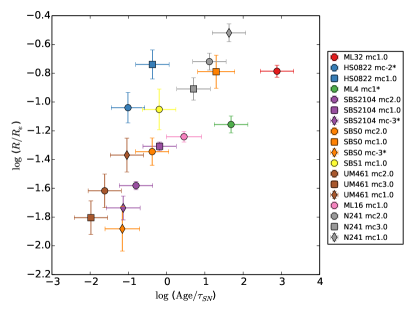
Figure 13.— Radius of the shell in terms of the radius of the star-forming region ($R/R_{e}$) versus $Age$ of the shell relative to the expected time-lag between SN explosions ($\tau_{SN}$). The color code and symbols have the same meaning as in previous figures, which is indicated in the inset.

Ages are estimated from the measured velocity and the estimated radius of the shell (Eq. [19]). These radii are small compared to the size of the star-forming regions. Figure 13 shows the radius relative to the effective radius of the region, with the typical ratio being around 10 % or smaller. Therefore, it is important to keep in mind, for interpreting the weak emission components in the wings of H$\alpha$, that there are one or several (probably non-concentric) expanding shells embedded in a large star-forming region. This substructure is common in giant HII regions, such as 30 Doradus in the large Magellanic cloud (e.g., Meaburn 1984; Sabbi et al. 2013; Camps-Fariña et al. 2015). Shells and holes appear in Hubble Space Telescope (HST) images of the large starburst in Kiso 5639, a tadpole galaxy very similar to the XMPs studied here (Elmegreen et al. 2016).

We do not see a dependence of the properties of the weak emission-line components on the mean metallicity of the starburst, except perhaps for the mass loading factor. Figure 14 shows the scatter plot of metallicity versus mass loading factor, and it hints at an increase of the factor with increasing metallicity. The trend may be coincidental, due to the small number of points in the plot. However, it may also indicate the contribution of stellar winds to the energy and momentum driving the observed expansion. The winds of massive stars can provide a total kynetic energy comparable to the energy released during their SN explosions (e.g., Fierlinger et al. 2016), and these radiation-pressure driven winds have mass loss rates that increase with increasing metallicity (e.g., Martins 2015).

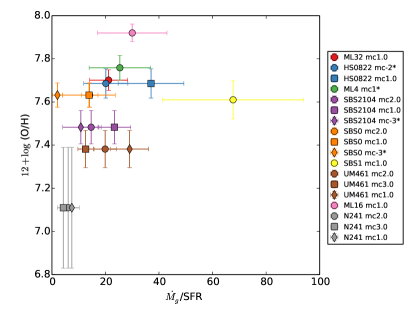
Figure 14.— Mean metallicity of the star-forming region versus mass loading factor. The color code and symbols have the same meaning as in previous figures, as indicated in the inset.

The metallicities represented in Fig. 14 correspond to the metallicity averaged over the starburst and, thus, due to the variation of metallicity across the star-forming region, their value is slightly higher than the values quoted in Paper I. ML16, the point of highest metallicity in Fig. 14, is also the galaxy with no detected metallicity inhomogeneity in Paper I.

5.2. Other interpretations

One can think of several alternatives to explain the existence of multiple paired emission-line components in the wings of H$\alpha$. The previous section analyzes the possibility of being produced by spatially-unresolved expanding shells driven by SN explosions. Here we discuss other options, such as (1) spatially-unresolved rotating structures, (2) spatially-resolved expanding shells, (3) bipolar outflows, (4) blown out spherical expansion leading to expanding rings, and (5) spatially-unresolved expanding shells driven by BH accretion feedback.

(1) Spatially-unresolved rotating disk-like structures. Rotation naturally produces double-horned profiles (e.g., Epstein 1964). Therefore, one of the possibilities to explain the existence of blue and red paired emission peaks is the presence of a gaseous structure rotating around a massive object. The mass of the required central object can be estimated from the size of the rotation structure and the velocity (Sect. 3.4). Figure 15 shows that the mass of the central object needs to be around three orders of magnitude larger than the gas mass involved in the motions, with central masses, $M_{\bullet}$, ranging from $10^{6}$–$10^{8}$ M_⊙. This mass turns out to be of the order of the stellar mass of the whole galaxy (Table 1), which rules out the stellar nature of the required central concentration. If, on the other hand, it were a BH, then it would have to have $M_{\bullet}\sim M_{\star}$, which is completely out of the so-called Magorrian-relationship between the central BH mass and the stellar mass of the galaxy, for which $M_{\bullet}/M_{\star}\sim 10^{-3}$ (e.g., Kormendy & Ho 2013). Thus, the exotic nature of the required central mass disfavors the interpretation of the weak emission in the wings of H$\alpha$ as caused by a disk orbiting around a massive central object, such as a BH.

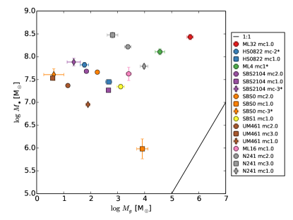
Figure 15.— Mass of the central object versus gas mass if the pairs of faint emission components are interpreted as caused by a gaseous disk orbiting around a central massive object. The solid line represents the one-to-one relationship. The masses of the required central objects turn out to be unrealistically large, which disfavors this interpretation. The color code and symbols have the same meaning as in previous figures, which is indicated in the inset.

(2) Spatially-resolved expanding shells. The inner part of a spatially resolved expanding shell also produces double peak emission-line profiles, since the outer parts of the shell, contributing to the line core, are excluded (e.g., Zuckerman 1987). We often see several pairs of emission peaks (Fig. 3a), therefore, this interpretation requires the existence of several resolved concentric shells, which is unrealistic since the first shell would have already swept the ISM around the center of the expansion. Moreover, the size of the shell is estimated to be smaller than the typical spatial resolution, so that the expanding regions cannot be spatially resolved.

(3) Bipolar outflows. Insofar as they comply with the energetics required to explain the observed motions, bipolar flows cannot be easily discarded. They create two-horned profiles, and several of them coexisting in the resolution element could explain the presence of multiple paired components. In fact, bipolar flows are extreme cases of non-spherically-symmetric shells, where double-horned line profiles appear naturally (e.g., Gill & O’Brien 1999).

(4) Blown out spherical expansion leading to expanding rings. If the radius of the shell exceeds the scale height of the disk of the galaxy, it may break up, leading to a ring-like expanding structure that produces two-horned profiles when observed edge-on. This possibility can be discarded since the ring would have to be as large as the disk thickness, which is incompatible with the small size of the expanding structures (Table 4).

(5) Spatially-unresolved expanding shells driven by BH accretion feedback. Energywise, intermediate mass BHs of $10^{5}~{}{\rm M}_{\odot}$ can also power the expanding shells that we characterize in Sect. 5.1 (see Eq. [24]). However, the observations also disfavor this option for a number of reasons. It is unclear how a primordial BH seed can coincide spatially with a star-forming region unless there are many such BHs lurking in the galaxy, or the BH is born in situ. $10^{5}~{}{\rm M}_{\odot}$ BHs can be produced by direct collapse in the early universe, but this explanation can be discarded, since they are very rare (e.g., van Wassenhove et al. 2010) and many of them are needed. On the other hand, $100~{}{\rm M}_{\odot}$ BHs are expected to be more common, left as remnants from population III stars formed in the early universe or even today (e.g., Kehrig et al. 2015). However, this alternative is also very unlikely, since HII regions are short-lived (a few tens of Myr; e.g., Leitherer et al. 1999), and a BH requires several hundred Myr of continuous feeding to grow from $100$ to $10^{5}~{}{\rm M}_{\odot}$ (see, e.g., Volonteri 2010). Finally, accreting BHs are expected to be luminous X-ray sources. Five of our XMPs were observed with the X-ray satellite Chandra: HS0822, SBS1, N241, SBS2109, and UM 461 (Kaaret et al. 2011; Prestwich et al. 2013). Only one of them shows a signal above the noise, namely, SBS1, with an X-ray luminosity around $10^{39}~{}{\rm erg\,s}^{-1}$. This level of emission is consistent with young SNe (e.g., Filho et al. 2004; González-Martín et al. 2006; Dwarkadas & Gruszko 2012).

6. The fate of the swept out material

Independently of the details on whether the shells are symmetric, or if they have internal extinction, the expanding shell model appears to be the best explanation to reproduce the weak emission features observed in the H$\alpha$ wings. One of the consequences of this interpretation is that the mass loading factor that we infer may be reflecting the feedback of the star formation process on the medium in, and around, the galaxy. The measured mass loading factor is very large, of the order of ten or larger (Fig. 11), which implies that for every solar mass of gas transformed into stars, at least ten times more gas is swept away from the region. How far this swept gas goes is impossible to tell from the data alone. However, a significant fraction may escape from the galaxy to the CGM and even the intergalactic medium (IGM). The speeds, larger than 100 km s^-1 and up to 400 km s^-1 (Table 4), likely exceed the escape velocity of the galaxy. The final fate of the gas depends on whether the gas pressure in the ISM of the galaxy suffices to slow down and confine the expansion. Even though we do not know the gas pressure of the ISM, it must be similar to the turbulent pressure in the star-forming region, so that the region is neither expanding nor shrinking considerably (the moderate global expansion observed in some cases is analyzed in the paragraph at the end of the section). The turbulent pressure scales with the square of the turbulent speed, and so does the pressure exerted by the shell on the ISM (e.g., Chandrasekhar 1951; Bonazzola et al. 1987). The measured turbulent velocities are of the order of 25 km s^-1 (see Table 2, and keep in mind that the quoted values are FWHM velocities rather than velocity dispersions), hence, provided that the HII region and the shell have similar densities, the ISM will not be able to confine a expanding shell with a speed of a few hundred km s^-1. A significant part of the matter in the shell may eventually escape from the galaxy. Martin (1999) made a qualitative estimate of the conditions for starburst-driven outflows to escape, finding that the gas flows out from galaxies with rotation smaller than 130 km s^-1, i.e., from our XMPs.

Under the hypothesis of expanding shell, it is possible to compute the column density to be expected if the shell material reaches the CGM. Assuming mass conservation, and if the shell geometry is maintained, the typical column density when the shell expands to a radius $R^{\prime}$ is,

$$N_{H}\simeq 7.9\times 10^{14}\,{\rm cm^{-2}}\,{{R}\over{10\,{\rm pc}}}\,{{n_{e}}\over{10^{2}\,{\rm cm^{-3}}}}\,\Big{[}{{R/R^{\prime}}\over{10^{-3}}}\Big{]}^{2},$$ (27)

where the electron density, $n_{e}$, and the radius, $R$, are those measured in the star-forming regions. Note that for the typical sizes and densities of our shells, and with expansion factors of the order of $10^{3}$ that transform pc-size shells into intergalactic size structures (from $R\simeq 10$ pc to $R^{\prime}\simeq 10$ kpc), the column densities predicted by Eq. (27) are of the order of $10^{15}\,{\rm cm^{-2}}$. This gas would be undetectable with current instrumentation, even if it were fully neutral. For example, a high-sensitivity survey such as HIPASS sets the limit at $4\times 10^{17}\,{\rm cm}^{-2}$ (Meyer et al. 2004), and values of $10^{17}\,{\rm cm}^{-2}$ will be achieved by SKA after a 1000 hour integration (de Blok et al. 2015). Moreover, at these low column densities the intergalactic ultraviolet (UV) background will keep the gas fully ionized, which makes it even more elusive. How long would it take for the gas to reach the CGM? Assuming that the original velocities are maintained, the time to reach the CGM is the expansion factor, $R^{\prime}/R$, times the $Age$ in Eq. (19). Given the $Age$ in Table 4 and $R^{\prime}/R\simeq 10^{3}$, the time-scale is of the order of 10 Myr, which is short compared to the time-scale for galaxy evolution. In summary, the shells that we observe in the star-forming regions are expected to reach the CGM, and may do it in a reasonable time-scale. Unfortunately, they would be undetectable with current instrumentation unless the expansion is more moderate than expected according to Eq. (27).

We show in Sect. 4 that some of the star-forming regions may be undergoing a global expansion, with a moderate velocity of around 15 km s^-1. The mass loss rate associated with this global expansion, $\dot{M}_{G}$, can also be estimated using Eq. (15), except that this time the global mass of the starburst, $M_{G}$, and the radius of the starburst, $R_{e}$, have to be considered. A simple substitution renders $\dot{M}_{G}$ in terms of the mass loss rate inferred for one of the weak components in the wings of H$\alpha$, i.e.,

$$\dot{M}_{G}/\dot{M}_{g}\simeq\varepsilon^{-1}\,(R/R_{e})\,(15~{}{\rm km\,s}^{-1}/v_{\rm out}),$$ (28)

where we have assumed $\Delta R/(R_{e}/3)\simeq R/R_{e}$, and $M_{g}/M_{G}\sim\varepsilon$. Using typical values for these parameters, $\varepsilon\simeq 5\times 10^{-3}$ (Table 4), $v_{\rm out}\simeq 150~{}{\rm km\,s}^{-1}$ (Table 4), and $R/R_{e}\sim 5\times 10^{-2}$ (Figure 13), one finds that the two mass loss rates are similar, i.e.,

$$\dot{M}_{G}/\dot{M}_{g}\sim 1.$$ (29)

One can repeat the exercise for the kinetic energy involved in the global expansion (Eq. [23]), which scales with the mass ratio and the square of the expansion velocities. Using the typical values given above, the two kinetic energies turn out to be similar too. This rough estimate leads to the conclusion that the mass loss rate and the kinetic energy involved in the global expansion of the star-forming region are similar to the values inferred for the emission features observed in the wings of H$\alpha$. The question arises as to whether the global expansion unbounds the gas in the starburst, and so may contribute to the global mass loss of the XMPs. As was the case with the small expanding shells discussed above, the answer to the question is very uncertain, and cannot be addressed resorting to our observational data alone. The fate of the gas depends on the unknown value of the ISM pressure. In contrast with the small shells, the expansion velocities are significantly smaller than the expected escape velocity. Moreover, the turbulent velocity of the galaxies is typically 40–50 km s^-1, and, hence, comparable, but larger, than the turbulent velocity in the star-forming region (see Fig. 6). Only if the density in the ISM of the XMPs is much lower than the density in the starburst, the starburst may be overpressureized and the mild observed expansion can drive gas through the ISM to large distances.

7. Conclusions

The XMP galaxies analyzed in Paper I are characterized by having a large star-forming region with a metal content lower than the rest of the galaxy. The presence of such chemical inhomogeneities suggests cosmological gas accretion as predicted in numerical simulations of galaxy formation. Cosmological gas accretion induces off-center giant star-forming clumps that gradually migrate toward the center of the galaxy disks (Ceverino et al. 2010; Mandelker et al. 2014). The star-forming clumps may be born in-situ or ex-situ. In the first case, the accreted gas builds up the gas reservoir in the disk to a point where disk instabilities set in and trigger star formation. In the second case, already formed clumps are incorporated into the disk. They may come with stars and dark matter, and thus, they are often indistinguishable from gas-rich minor mergers (Mandelker et al. 2014). Since they feed from metal-poor gas, the star-forming clumps are more metal-poor than their immediate surroundings (Ceverino et al. 2016). In order to complement the chemical analysis carried out in Paper I, this second paper studies the kinematic properties of the ionized gas forming stars in the XMP galaxies. We study nine objects (Table 1) with a spectral resolution of the order of 7500, equivalent to 40 km s^-1 in H$\alpha$.

Most XMPs have a measurable rotation velocity, with a rotation amplitude which is only a few tens of km s^-1 (Fig. 5). All rotation curves present small-scale velocity irregularities, often with an amplitude comparable to the velocity gradient across the whole galaxy. On top of the large-scale motion, the galaxies also present turbulent motions of typically 50 km s^-1 FWHM (see Fig. 6 and Table 2), and, therefore, larger than the rotational velocities.

Observations suggest that the main star-forming region of the galaxy (Fig. 1) moves coherently within the host galaxy. The velocity is constant (Fig. 7), so that the region moves as a single unit within the global rotation pattern of the galaxy. In addition, the velocity dispersion in some of these large star-forming clumps increases toward the center-side of the galaxy. The excess velocity dispersion on the center-side may indicate an intensification of the turbulence of the gas that collides with the ISM of the host galaxy, as if the clumps were inspiraling toward the galaxy center. This migration to the galaxy center is expected from tidal forces acting upon massive gas clumps (see, e.g., Elmegreen et al. 2008, 2012a; Bournaud et al. 2008; Ceverino et al. 2016), and the large starbursts in our XMPs may be going through the process at this moment. In some other cases, the velocity dispersion has a local maximum at the core of the star-forming region, which suggests a global expansion of the whole region, with a moderate speed of around 15 km s^-1. Sometimes the velocity dispersion presents a minimum at the core, which may reflect a past global expansion that washed out part of the turbulent motions.

We find no obvious relationship between the kinematic properties and the metallicity drops, except for the already known correlation between the presence of a starburst and the decrease in metallicity. We do find, however, a significant lack of correlation between the metallicity and the N/O ratio (Fig. 8), which is consistent with the gas accretion scenario. If the accretion of metal-poor gas is fueling the observed starbursts, then the fresh gas reduces the metallicity (i.e., O/H), but it cannot modify the pre-existing ratio between metals (e.g., Amorín et al. 2010, 2012), forcing the N/O ratio to be similar inside and outside the starburst.

The H$\alpha$ line profile often shows a number of faint emission features, Doppler-shifted with respect to the central component. Their amplitudes are typically a few percent of the main component (Fig. 3), with the velocity shifts being between 100 and 400 km s^-1 (Table 4). The components are often paired, so that red and blue peaks, with similar amplitudes and shifts, appear simultaneously. The red components tend to be slightly fainter, however. Assuming that the emission is produced by recombination of H, we have estimated the gas mass in motion, which turns out to be in the range between 10 and $10^{5}~{}{\rm M}_{\odot}$ (Table 4 and Fig. 10). Assuming that the Doppler shifts are produced by an expanding shell-like structure, we infer a mass loss rate between $10^{-2}$ and a few ${\rm M}_{\odot}\,{\rm yr}^{-1}$. Given the observed SFR, the mass loss rate yields a mass loading factor (defined as the mass loss rate divided by the SFR) typically in excess of 10. Large mass loading factors are indeed expected from numerical simulations (e.g., Peeples & Shankar 2011; Davé et al. 2012; Oppenheimer et al. 2012), and they reflect the large feedback of the star formation process on the surrounding medium. Numerical simulations predict that low mass galaxies are extremely inefficient in using their gas, most of which returns to the IGM without being processed through the stellar mechanism. Since the measured expansion velocities exceed by far the rotational and turbulent velocities, we argue in Sect. 5.2 that the gas involved in the expansion is bound to escape from the galaxy disk, reaching the CGM and possibly the IGM. Therefore, the large mass loading factors that we measure support and constrain the predictions from numerical simulations. We have estimated the H column density to be expected when the shell material reaches the CGM, and it turns out to be around $10^{15}$ cm^-2. Even if all the H were neutral, this is undetectably small with present technology. Moreover, at these low column densities, all H is expected to be ionized by the cosmic UV background. Even if the IGM of the XMPs were filled by expanding shells from previous starbursts, they would be extremely elusive observationally.

From an energetic point of view, the observed motions involve energies between $10^{49}$ and $10^{52}$ erg, which are in the range of the kinetic energy released by a core-collapse SN ($\sim 10^{51}$ erg). The low-end energy requires that only part of the SN kinetic energy drives the observed expansion, whereas the high-end energy requires several SNe going off quasi-simultaneously. The observed SFRs allow for the required number of SNe, and the estimated age of the shells ($10^{4}$–$10^{6}$ yr; Table 4) is also consistent with the expected SN rate. Other alternatives to explain the weak emission peaks in the wings of H$\alpha$, like BH driving the motions or the expansion, can be discarded using physical arguments (Sect. 5.2).

Some of the data suggest a moderate global expansion of the star-forming regions (Sect. 6). Even if the expansion velocity is small (around 15 km s^-1), the motion involves the mass of the whole region, and, hence, the associated mass loss rate and kinetic energy turn out to be similar to those carried away by the fast-moving secondary components. Thus, global expansion may also be important in setting up the mass and energy budgets associated with star formation feedback.

High redshift clumpy galaxies are probably growing through a cosmological gas accretion process similar to the one experienced by XMPs. However, the physical conditions at high and low redshifts differ (e.g., the gas accretion rates are larger at high redshifts), so do the observational biases affecting XMPs and high-redshift clumpies (e.g., low-mass galaxies are undetectable at high redshift). Therefore, addressing the issue of whether XMPs are low-mass analogues of high-redshift clumpies is complicated, and so goes beyond the scope of our work. However, because of their probable common physics, it is interesting to point out some of the similarities and differences of the two samples. As in the case of XMPs, some clumpy galaxies show metallicity drops associated with enhanced star-formation activity (Cresci et al. 2010; Troncoso et al. 2014). High redshift galaxies are significantly more massive than XMPs. Using as reference for high redshift galaxies (1.3–2.6) the SINS sample (Förster Schreiber et al. 2009), the stellar mass of the high-redshift objects ($10^{9.5}$–$10^{11}$ $M_{\odot}$) is three orders of magnitude larger than the mass of XMPs ($10^{6}$–$10^{8.5}$ $M_{\odot}$; Table 1). This difference in stellar mass shows in dynamical mass too, with rotational velocities between 100 and 260 km s^-1 at high redshift. We cannot directly compare the rotational velocities of XMPs with these values since we cannot corrected for inclination, however, the uncorrected values go from zero to 30 km s^-1 (see Fig. 5). The velocity dispersion in XMPs ranges from 10 and 20 km s^-1 (corresponding to FWHM between 25 and 50 km s^-1; see Fig. 6), whereas it is between 50 and 200 km s^-1 at high-redshift (Förster Schreiber et al. 2009). The high redshift objects have a ratio between rotational velocity and velocity dispersion between 0.5 and one (Förster Schreiber et al. 2009). XMPs seem to have similar ratios, even though we cannot be more precise since the measured rotation in XMPs is affected by inclination. The total SFRs are very different (10 – 500 $M_{\odot}$ yr^-1 at high redshift and 0.001 – 0.1 $M_{\odot}$ yr^-1 in XMPs), but the surface star-formation rates are not; they go from 0.01 to 10 $M_{\odot}$ yr^-1 kpc^-2 at high redshift (e.g., Fisher et al. 2016) and from 0.005 to 0.8 $M_{\odot}$ yr^-1 kpc^-2 in XMPs (Paper I). Mass loading factors are one order of magnitude larger in XMPs than those inferred for high-redshift clumpy galaxies (Sect. 5; see also Newman et al. 2012), a difference that we attribute to their very different masses. However, the differences of size between the expanding regions of clumpies and XMPs may also play a role (see Eq. [15]). Local UV bright clumply galaxies (Elmegreen et al. 2012b) are often XMPs with metallicity drops (Sánchez Almeida et al. 2013), and we know that their star-forming clumps resemble those in high-redshift cumplies in terms of total SFR, clump mass, and stellar mass surface density (Elmegreen et al. 2013).

Appendix A Emission of an expanding dusty shell of gas

The emission of a uniform shell produces a top-hat line profile that is not consistent with the two-horned profiles observed in the wings of H$\alpha$ (Fig. 3). However, if the shell has some internal extinction, then it preferentially absorbs photons emerging from the regions where the line-of-sight (LOS) tends to be parallel to the surface of the shell. Those are the regions of small Doppler shifts that contribute to the line center, thus creating a two-horned profile.

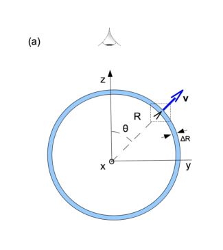
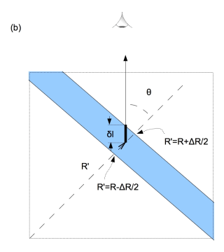
Figure 16.— Schematic used to compute the emission-line profile of an expanding dusty shell of radius $R$ and width $\Delta R$. (a) Projection of the shell in the Y-Z plane, with Z in the direction along the LOS. The velocity vector, ${\bf v}$, in the direction set by $\theta$ is shown as a blue solid-line arrow. (b) Zoom-in of the region enclosed by the dotted-line rectangle in (a). The length along the LOS traversed by the photons emitted at coordinates ($\theta$, $R^{\prime}$) is denoted as $\delta l$, with $\delta l=(R+\Delta R/2-R^{\prime})/\cos\theta$.

The effect can be readily shown assuming an expanding shell of radius $R$ and width $\Delta R$, as shown in Fig. 16a. The velocity along the LOS, $v_{z}$, only depends on the inclination angle, $\theta$,

$$v_{z}=v\,\cos\theta.$$ (A1)

Therefore, the line profile, $I(v_{z})$, is just the total energy emitted with velocity between $v_{z}$ and $v_{z}+\Delta v_{z}$, divided by $\Delta v_{z}$. Because of Eq. (A1), it is proportional to the energy emitted by the ring of the shell with inclination angles between $\theta$ and $\theta+\Delta\theta$, i.e.,

$$\Delta s=\int_{0}^{2\pi}\int_{R-\Delta R/2}^{R+\Delta R/2}\int_{\theta}^{\theta+\Delta\theta}\,\epsilon\,\sin\theta^{\prime}\,R^{\prime 2}\,d\phi\,dR^{\prime}\,d\theta^{\prime},$$ (A2)

where $R$ is the radius of the shell of width $\Delta R$, $\phi$ is the azimuth in spherical coordinates, and $\epsilon$ stands for the emission per unit volume. Assuming the shell to be small enough ($\Delta R\ll R$), then

$$\Delta s\simeq 2\pi\,R^{2}\,\sin\theta\,\Delta\theta\,\int_{R-\Delta R/2}^{R+\Delta R/2}\epsilon\,dR^{\prime}.$$ (A3)

According to the definition of $I(v_{z})$,

$$I(v_{z})=\Big{|}{{\Delta s}\over{\Delta v_{z}}}\Big{|}=\Big{|}{{\Delta s}\over{\Delta\theta}}\,{{\Delta\theta}\over{\Delta v_{z}}}\Big{|}\simeq\Big{|}{{\Delta s}\over{\Delta\theta}}\,\Big{(}{{dv_{z}}\over{d\theta}}\Big{)}^{-1}\Big{|},$$ (A4)

so Eqs. (A1), (A3) and (A4) yield,

$$I(v_{z})\simeq 2\pi\,R^{2}\,v^{-1}\,\int_{R-\Delta R/2}^{R+\Delta R/2}\epsilon\,dR^{\prime},$$ (A5)

which holds only for $|v_{z}|\leq v$. Outside this range of velocities, $\Delta s$ is equal to zero, and so is $I(v_{z})$.

In the case that $\epsilon$ is constant, then $I(v_{z})$ is also constant (Eq. [A5]), leading to the top-hat line profiles expected from an optically thin expanding shell. We will consider the case where the emission is constant, $\epsilon_{0}$, but the shell absorbs part of the emitted photons due to internal extinction, $\beta$, i.e.,

$$\epsilon=\epsilon_{0}\,\exp(-\beta\delta l),$$ (A6)

with

$$\delta l(R^{\prime})\simeq{{R+\Delta R/2-R^{\prime}}\over{\cos\theta}},$$ (A7)

as shown in Fig. 16b. For the moment, we have assumed that the emission occurs in the upper cap only. Using Eqs. (A5), (A6), and (A7),

$$I(v_{z})\simeq I_{0}\,{{\cos\theta}\over{\beta\Delta R}}\Big{[}1-\exp(-\beta\Delta R/\cos\theta)\Big{]},$$ (A8)

$$\cos\theta\geq 0,{\rm~{}~{}~{}~{}~{}or~{}~{}~{}~{}~{}}v_{z}\geq 0,$$

with $I_{0}$ the emitted intensity if there were no extintion ($\beta\longrightarrow 0$),

$$I_{0}=2\pi\,R^{2}\,\Delta R\,\,v^{-1}\,\epsilon_{0}.$$ (A9)

The case of the lower cap is similar, except that one has to consider the additional absorption produced by the upper cap. In this other case,

$$I(v_{z})\simeq I_{0}\,{{|\cos\theta|}\over{\beta\Delta R}}\Big{[}1-\exp(-\beta\Delta R/|\cos\theta|)\Big{]}\,\exp(-\beta\Delta R/|\cos\theta|),$$ (A10)

with

$$\cos\theta<0{\rm~{}~{}~{}~{}~{}or~{}~{}~{}~{}~{}}v_{z}<0.$$

The typical values of the extinction coefficient at H$\beta$ in XMPs are between $0.1$ and $0.9$ (Sánchez Almeida et al. 2016). These values were inferred from the Balmer decrement in Sloan Digital Sky Survey (SDSS) spectra of XMPs. If we use them to represent the total extintion in the shell, then $0.15<\beta\,\Delta R<1.5$, where we have considered the differential extintion between H$\alpha$ and H$\beta$ using the extinction law in the Milky Way by Cardelli et al. (1989). The dashed lines in Fig. 17 show examples of the line profiles resulting from Eqs. (A8) and (A10). They represent extinctions that cover the range of values mentioned above. We show the original profiles (dashed lines) plus their convolution with a Gaussian that represents the finite resolution of the observation (solid lines). The width of the Gaussian has been chosen so that, if it represents our WHT observations (FWHM $\sim 40~{}$km s^-1), then the expansion velocities of the shells are similar to the speeds of the multiple components analyzed in Sect. 5. One can see the two-horned shape, with a redshifted lobe that is smaller than the blushifted lobe; the redshifted photons come from the lower cap of the shell, so that they are also extincted by the upper cap (we have flipped the sign of the abscissa axis in Fig. 17, so that positive corresponds to redshift, as usual).

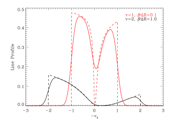
Figure 17.— Line profiles expected from an expanding dusty shell. They portray both weak internal extinction ($\beta\Delta R=0.1$; profiles in red), and significant internal extinction ($\beta\Delta R=1.0$, profiles in black). Red and black lines also differ in the expansion speed $v$, as shown in the inset. We include the profiles predicted by Eqs. (A8) and (A10) (dashed lines), together with these profiles convolved with a Gaussian to represent the finite spectral resolution of the spectrograph (solid lines). We assume the FWHM of the Gaussian to be 0.35 in the dimensionless velocity scale. If this value is ascribed to the resolution of our observation ($\sim 40~{}$km s^-1), then the expansion speeds for the shells giving rise to the red and black profiles are 110 km s^-1 and 220 km s^-1, respectively. Abscissae show $-v_{z}$ rather than $v_{z}$ so that the positive values correspond to redshifts.

The model in Eqs. (A8) and (A10) also predicts the fraction of emitted light lost by internal absorption. For the two profiles shown in Fig. 17, the fraction of light that emerges is 74 % and 24 % of the emitted light for the red and black profiles, respectively.

References

- Alam et al. (2015) Alam, S., Albareti, F. D., Allende Prieto, C., Anders, F., Anderson, S. F., Anderton, T., Andrews, B. H., Armengaud, E., Aubourg, É., Bailey, S., & et al. 2015, ApJS, 219, 12
- Amorín et al. (2015) Amorín, R., Pérez-Montero, E., Contini, T., Vílchez, J. M., Bolzonella, M., Tasca, L. A. M., Lamareille, F., Zamorani, G., Maier, C., Carollo, C. M., Kneib, J.-P., Le Fèvre, O., Lilly, S., Mainieri, V., Renzini, A., Scodeggio, M., Bardelli, S., Bongiorno, A., Caputi, K., Cucciati, O., de la Torre, S., de Ravel, L., Franzetti, P., Garilli, B., Iovino, A., Kampczyk, P., Knobel, C., Kovač, K., Le Borgne, J.-F., Le Brun, V., Mignoli, M., Pellò, R., Peng, Y., Presotto, V., Ricciardelli, E., Silverman, J. D., Tanaka, M., Tresse, L., Vergani, D., & Zucca, E. 2015, A&A, 578, A105
- Amorín et al. (2012) Amorín, R., Pérez-Montero, E., Vílchez, J. M., & Papaderos, P. 2012, ApJ, 749, 185
- Amorín et al. (2010) Amorín, R. O., Pérez-Montero, E., & Vílchez, J. M. 2010, ApJ, 715, L128
- Asplund et al. (2009) Asplund, M., Grevesse, N., Sauval, A. J., & Scott, P. 2009, ARA&A, 47, 481
- Bastian et al. (2006) Bastian, N., Emsellem, E., Kissler-Patig, M., & Maraston, C. 2006, A&A, 445, 471
- Berg et al. (2012) Berg, D. A., Skillman, E. D., Marble, A. R., van Zee, L., Engelbracht, C. W., Lee, J. C., Kennicutt, Jr., R. C., Calzetti, D., Dale, D. A., & Johnson, B. D. 2012, ApJ, 754, 98
- Binney & Tremaine (2008) Binney, J., & Tremaine, S. 2008, Galactic Dynamics: Second Edition (Princeton University Press)
- Birnboim & Dekel (2003) Birnboim, Y., & Dekel, A. 2003, MNRAS, 345, 349
- Bonazzola et al. (1987) Bonazzola, S., Heyvaerts, J., Falgarone, E., Perault, M., & Puget, J. L. 1987, A&A, 172, 293
- Bournaud et al. (2008) Bournaud, F., Daddi, E., Elmegreen, B. G., Elmegreen, D. M., Nesvadba, N., Vanzella, E., Di Matteo, P., Le Tiran, L., Lehnert, M., & Elbaz, D. 2008, A&A, 486, 741
- Bournaud et al. (2014) Bournaud, F., Perret, V., Renaud, F., Dekel, A., Elmegreen, B. G., Elmegreen, D. M., Teyssier, R., Amram, P., Daddi, E., Duc, P.-A., Elbaz, D., Epinat, B., Gabor, J. M., Juneau, S., Kraljic, K., & Le Floch’, E. 2014, ApJ, 780, 57
- Camps-Fariña et al. (2015) Camps-Fariña, A., Zaragoza-Cardiel, J., Beckman, J. E., Font, J., García-Lorenzo, B., Erroz-Ferrer, S., & Amram, P. 2015, MNRAS, 447, 3840
- Cardelli et al. (1989) Cardelli, J. A., Clayton, G. C., & Mathis, J. S. 1989, ApJ, 345, 245
- Carniani et al. (2015) Carniani, S., Marconi, A., Maiolino, R., Balmaverde, B., Brusa, M., Cano-Díaz, M., Cicone, C., Comastri, A., Cresci, G., Fiore, F., Feruglio, C., La Franca, F., Mainieri, V., Mannucci, F., Nagao, T., Netzer, H., Piconcelli, E., Risaliti, G., Schneider, R., & Shemmer, O. 2015, A&A, 580, A102
- Ceverino et al. (2010) Ceverino, D., Dekel, A., & Bournaud, F. 2010, MNRAS, 404, 2151
- Ceverino et al. (2016) Ceverino, D., Sánchez Almeida, J., Muñoz Tuñón, C., Dekel, A., Elmegreen, B. G., Elmegreen, D. M., & Primack, J. 2016, MNRAS, 457, 2605
- Chandrasekhar (1951) Chandrasekhar, S. 1951, Proceedings of the Royal Society of London Series A, 210, 18
- Cid Fernandes & Terlevich (1994) Cid Fernandes, R., & Terlevich, R. 1994, Line profiles in compact supernova remnants and active galactic nuclei., ed. G. Tenorio-Tagle
- Cresci et al. (2010) Cresci, G., Mannucci, F., Maiolino, R., Marconi, A., Gnerucci, A., & Magrini, L. 2010, Nature, 467, 811
- Dalcanton & Stilp (2010) Dalcanton, J. J., & Stilp, A. M. 2010, ApJ, 721, 547
- Davé et al. (2012) Davé, R., Finlator, K., & Oppenheimer, B. D. 2012, MNRAS, 421, 98
- de Avillez & Mac Low (2002) de Avillez, M. A., & Mac Low, M.-M. 2002, ApJ, 581, 1047
- de Blok et al. (2015) de Blok, W. J. G., Fraternali, F., Heald, G. H., Adams, E. A. K., Bosma, A., Koribalski, B. S., & the HI Science Working Group. 2015, ArXiv e-prints
- Dekel et al. (2009) Dekel, A., Birnboim, Y., Engel, G., Freundlich, J., Goerdt, T., Mumcuoglu, M., Neistein, E., Pichon, C., Teyssier, R., & Zinger, E. 2009, Nature, 457, 451
- Dwarkadas & Gruszko (2012) Dwarkadas, V. V., & Gruszko, J. 2012, MNRAS, 419, 1515
- Elmegreen et al. (2008) Elmegreen, B. G., Bournaud, F., & Elmegreen, D. M. 2008, ApJ, 688, 67
- Elmegreen et al. (2013) Elmegreen, B. G., Elmegreen, D. M., Sánchez Almeida, J., Muñoz-Tuñón, C., Dewberry, J., Putko, J., Teich, Y., & Popinchalk, M. 2013, ApJ, 774, 86
- Elmegreen et al. (2012a) Elmegreen, B. G., Zhang, H.-X., & Hunter, D. A. 2012a, ApJ, 747, 105
- Elmegreen et al. (2012b) Elmegreen, D. M., Elmegreen, B. G., Sánchez Almeida, J., Muñoz-Tuñón, C., Putko, J., & Dewberry, J. 2012b, ApJ, 750, 95
- Elmegreen et al. (2016) Elmegreen, D. M., Elmegreen, B. G., Sanchez Almeida, J., Munoz-Tunon, C., Mendez-Abreu, J., Gallagher, J. S., Rafelski, M., Filho, M., & Ceverino, D. 2016, ArXiv e-prints
- Emerson (1996) Emerson, D. 1996, Interpreting Astronomical Spectra, 472
- Epstein (1964) Epstein, E. E. 1964, AJ, 69, 521
- Ferrara et al. (2014) Ferrara, A., Salvadori, S., Yue, B., & Schleicher, D. 2014, MNRAS, 443, 2410
- Fierlinger et al. (2016) Fierlinger, K. M., Burkert, A., Ntormousi, E., Fierlinger, P., Schartmann, M., Ballone, A., Krause, M. G. H., & Diehl, R. 2016, MNRAS, 456, 710
- Filho et al. (2004) Filho, M. E., Fraternali, F., Markoff, S., Nagar, N. M., Barthel, P. D., Ho, L. C., & Yuan, F. 2004, A&A, 418, 429
- Filho et al. (2013) Filho, M. E., Winkel, B., Sánchez Almeida, J., Aguerri, J. A., Amorín, R., Ascasibar, Y., Elmegreen, B. G., Elmegreen, D. M., Gomes, J. M., Humphrey, A., Lagos, P., Morales-Luis, A. B., Muñoz-Tuñón, C., Papaderos, P., & Vílchez, J. M. 2013, A&A, 558, A18
- Fisher et al. (2016) Fisher, D. B., Glazebrook, K., Damjanov, I., Abraham, R. G., Obreschkow, D., Wisnioski, E., Bassett, R., Green, A., & McGregor, P. 2016, MNRAS
- Förster Schreiber et al. (2009) Förster Schreiber, N. M., Genzel, R., Bouché, N., Cresci, G., Davies, R., Buschkamp, P., Shapiro, K., Tacconi, L. J., Hicks, E. K. S., Genel, S., Shapley, A. E., Erb, D. K., Steidel, C. C., Lutz, D., Eisenhauer, F., Gillessen, S., Sternberg, A., Renzini, A., Cimatti, A., Daddi, E., Kurk, J., Lilly, S., Kong, X., Lehnert, M. D., Nesvadba, N., Verma, A., McCracken, H., Arimoto, N., Mignoli, M., & Onodera, M. 2009, ApJ, 706, 1364
- Frank et al. (2002) Frank, J., King, A., & Raine, D. J. 2002, Accretion Power in Astrophysics: Third Edition, 398
- Gill & O’Brien (1999) Gill, C. D., & O’Brien, T. J. 1999, MNRAS, 307, 677
- González-Martín et al. (2006) González-Martín, O., Masegosa, J., Márquez, I., Guerrero, M. A., & Dultzin-Hacyan, D. 2006, A&A, 460, 45
- Hinojosa-Goñi et al. (2016) Hinojosa-Goñi, R., Muñoz-Tuñón, C., & Méndez-Abreu, J. 2016, ArXiv e-prints
- Hinz et al. (2001) Hinz, J. L., Rix, H.-W., & Bernstein, G. M. 2001, AJ, 121, 683
- Israelian et al. (2004) Israelian, G., Ecuvillon, A., Rebolo, R., García-López, R., Bonifacio, P., & Molaro, P. 2004, A&A, 421, 649
- Izotov et al. (2009) Izotov, Y. I., Guseva, N. G., Fricke, K. J., & Papaderos, P. 2009, A&A, 503, 61
- Izotov et al. (2012) Izotov, Y. I., Thuan, T. X., & Guseva, N. G. 2012, A&A, 546, A122
- James et al. (2015) James, B. L., Koposov, S., Stark, D. P., Belokurov, V., Pettini, M., & Olszewski, E. W. 2015, MNRAS, 448, 2687
- Kaaret et al. (2011) Kaaret, P., Schmitt, J., & Gorski, M. 2011, ApJ, 741, 10
- Kasen & Woosley (2009) Kasen, D., & Woosley, S. E. 2009, ApJ, 703, 2205
- Kehrig et al. (2015) Kehrig, C., Vílchez, J. M., Pérez-Montero, E., Iglesias-Páramo, J., Brinchmann, J., Kunth, D., Durret, F., & Bayo, F. M. 2015, ApJ, 801, L28
- Keller et al. (2014) Keller, B. W., Wadsley, J., Benincasa, S. M., & Couchman, H. M. P. 2014, MNRAS, 442, 3013
- Kennicutt & Evans (2012) Kennicutt, R. C., & Evans, N. J. 2012, ARA&A, 50, 531
- Kennicutt (1998) Kennicutt, Jr., R. C. 1998, ARA&A, 36, 189
- Kereš et al. (2005) Kereš, D., Katz, N., Weinberg, D. H., & Davé, R. 2005, MNRAS, 363, 2
- Kormendy & Ho (2013) Kormendy, J., & Ho, L. C. 2013, ARA&A, 51, 511
- Kunth & Östlin (2000) Kunth, D., & Östlin, G. 2000, A&A Rev., 10, 1
- Lang (1999) Lang, K. R. 1999, Astrophysical formulae
- Leitherer et al. (1999) Leitherer, C., Schaerer, D., Goldader, J. D., Delgado, R. M. G., Robert, C., Kune, D. F., de Mello, D. F., Devost, D., & Heckman, T. M. 1999, ApJS, 123, 3
- Levesque et al. (2011) Levesque, E. M., Berger, E., Soderberg, A. M., & Chornock, R. 2011, ApJ, 739, 23
- Maiolino et al. (2012) Maiolino, R., Gallerani, S., Neri, R., Cicone, C., Ferrara, A., Genzel, R., Lutz, D., Sturm, E., Tacconi, L. J., Walter, F., Feruglio, C., Fiore, F., & Piconcelli, E. 2012, MNRAS, 425, L66
- Mandelker et al. (2014) Mandelker, N., Dekel, A., Ceverino, D., Tweed, D., Moody, C. E., & Primack, J. 2014, MNRAS, 443, 3675
- Martin (1971) Martin, B. R. 1971, Statistics for physicists
- Martin (1999) Martin, C. L. 1999, ApJ, 513, 156
- Martin et al. (2012) Martin, C. L., Shapley, A. E., Coil, A. L., Kornei, K. A., Bundy, K., Weiner, B. J., Noeske, K. G., & Schiminovich, D. 2012, ApJ, 760, 127
- Martins (2015) Martins, F. 2015, in SF2A-2015: Proceedings of the Annual meeting of the French Society of Astronomy and Astrophysics, ed. F. Martins, S. Boissier, V. Buat, L. Cambrésy, & P. Petit, 343–348
- Meaburn (1984) Meaburn, J. 1984, MNRAS, 211, 521
- Meyer et al. (2004) Meyer, M. J., Zwaan, M. A., Webster, R. L., Staveley-Smith, L., Ryan-Weber, E., Drinkwater, M. J., Barnes, D. G., Howlett, M., Kilborn, V. A., Stevens, J., Waugh, M., Pierce, M. J., Bhathal, R., de Blok, W. J. G., Disney, M. J., Ekers, R. D., Freeman, K. C., Garcia, D. A., Gibson, B. K., Harnett, J., Henning, P. A., Jerjen, H., Kesteven, M. J., Knezek, P. M., Koribalski, B. S., Mader, S., Marquarding, M., Minchin, R. F., O’Brien, J., Oosterloo, T., Price, R. M., Putman, M. E., Ryder, S. D., Sadler, E. M., Stewart, I. M., Stootman, F., & Wright, A. E. 2004, MNRAS, 350, 1195
- Morales-Luis et al. (2011) Morales-Luis, A. B., Sánchez Almeida, J., Aguerri, J. A. L., & Muñoz-Tuñón, C. 2011, ApJ, 743, 77
- Murray & Chang (2015) Murray, N., & Chang, P. 2015, ApJ, 804, 44
- Newman et al. (2012) Newman, S. F., Genzel, R., Förster-Schreiber, N. M., Shapiro Griffin, K., Mancini, C., Lilly, S. J., Renzini, A., Bouché, N., Burkert, A., Buschkamp, P., Carollo, C. M., Cresci, G., Davies, R., Eisenhauer, F., Genel, S., Hicks, E. K. S., Kurk, J., Lutz, D., Naab, T., Peng, Y., Sternberg, A., Tacconi, L. J., Vergani, D., Wuyts, S., & Zamorani, G. 2012, ApJ, 761, 43
- Newville et al. (2014) Newville, M., Stensitzki, T., Allen, D. B., & Ingargiola, A. 2014, LMFIT: Non-Linear Least-Square Minimization and Curve-Fitting for Python
- Oppenheimer et al. (2012) Oppenheimer, B. D., Davé, R., Katz, N., Kollmeier, J. A., & Weinberg, D. H. 2012, MNRAS, 420, 829
- Osterbrock (1974) Osterbrock, D. E. 1974, Astrophysics of gaseous nebulae
- Pacucci et al. (2016) Pacucci, F., Ferrara, A., Grazian, A., Fiore, F., Giallongo, E., & Puccetti, S. 2016, MNRAS, 459, 1432
- Papaderos et al. (2008) Papaderos, P., Guseva, N. G., Izotov, Y. I., & Fricke, K. J. 2008, A&A, 491, 113
- Papaderos et al. (2006) Papaderos, P., Izotov, Y. I., Guseva, N. G., Thuan, T. X., & Fricke, K. J. 2006, A&A, 454, 119
- Peeples & Shankar (2011) Peeples, M. S., & Shankar, F. 2011, MNRAS, 417, 2962
- Pérez-Montero (2014) Pérez-Montero, E. 2014, MNRAS, 441, 2663
- Pérez-Montero & Contini (2009) Pérez-Montero, E., & Contini, T. 2009, MNRAS, 398, 949
- Pérez-Montero et al. (2013) Pérez-Montero, E., Contini, T., Lamareille, F., Maier, C., Carollo, C. M., Kneib, J.-P., Le Fèvre, O., Lilly, S., Mainieri, V., Renzini, A., Scodeggio, M., Zamorani, G., Bardelli, S., Bolzonella, M., Bongiorno, A., Caputi, K., Cucciati, O., de la Torre, S., de Ravel, L., Franzetti, P., Garilli, B., Iovino, A., Kampczyk, P., Knobel, C., Kovač, K., Le Borgne, J.-F., Le Brun, V., Mignoli, M., Pellò, R., Peng, Y., Presotto, V., Ricciardelli, E., Silverman, J. D., Tanaka, M., Tasca, L. A. M., Tresse, L., Vergani, D., & Zucca, E. 2013, A&A, 549, A25
- Press et al. (1986) Press, W. H., Flannery, B. P., & Teukolsky, S. A. 1986, Numerical recipes. The art of scientific computing
- Prestwich et al. (2013) Prestwich, A. H., Tsantaki, M., Zezas, A., Jackson, F., Roberts, T. P., Foltz, R., Linden, T., & Kalogera, V. 2013, ApJ, 769, 92
- Putman et al. (2012) Putman, M. E., Peek, J. E. G., & Joung, M. R. 2012, ARA&A, 50, 491
- Read et al. (2016) Read, J. I., Iorio, G., Agertz, O., & Fraternali, F. 2016, MNRAS, 462, 3628
- Robertson & Goldreich (2012) Robertson, B., & Goldreich, P. 2012, ApJ, 750, L31
- Sabbi et al. (2013) Sabbi, E., Anderson, J., Lennon, D. J., van der Marel, R. P., Aloisi, A., Boyer, M. L., Cignoni, M., de Marchi, G., de Mink, S. E., Evans, C. J., Gallagher, III, J. S., Gordon, K., Gouliermis, D. A., Grebel, E. K., Koekemoer, A. M., Larsen, S. S., Panagia, N., Ryon, J. E., Smith, L. J., Tosi, M., & Zaritsky, D. 2013, AJ, 146, 53
- Salucci et al. (2007) Salucci, P., Lapi, A., Tonini, C., Gentile, G., Yegorova, I., & Klein, U. 2007, MNRAS, 378, 41
- Sánchez Almeida et al. (2014a) Sánchez Almeida, J., Elmegreen, B. G., Muñoz-Tuñón, C., & Elmegreen, D. M. 2014a, A&A Rev., 22, 71
- Sánchez Almeida et al. (2015) Sánchez Almeida, J., Elmegreen, B. G., Muñoz-Tuñón, C., Elmegreen, D. M., Pérez-Montero, E., Amorín, R., Filho, M. E., Ascasibar, Y., Papaderos, P., & Vílchez, J. M. 2015, ApJ, 810, L15 (Paper I)
- Sánchez Almeida & et al. (2016b) Sánchez Almeida, J., & et al. 2016b, On the dearth of ultra-faint XMPs, in preparation
- Sánchez Almeida et al. (2014b) Sánchez Almeida, J., Morales-Luis, A. B., Muñoz-Tuñón, C., Elmegreen, D. M., Elmegreen, B. G., & Méndez-Abreu, J. 2014b, ApJ, 783, 45
- Sánchez Almeida et al. (2013) Sánchez Almeida, J., Muñoz-Tuñón, C., Elmegreen, D. M., Elmegreen, B. G., & Méndez-Abreu, J. 2013, ApJ, 767, 74
- Sánchez Almeida et al. (2016) Sánchez Almeida, J., Pérez-Montero, E., Morales-Luis, A. B., Muñoz-Tuñón, C., García-Benito, R., Nuza, S. E., & Kitaura, F. S. 2016, ApJ, 819, 110
- Sancisi et al. (2008) Sancisi, R., Fraternali, F., Oosterloo, T., & van der Hulst, T. 2008, A&A Rev., 15, 189
- Schweizer (1979) Schweizer, F. 1979, PASP, 91, 149
- Skillman et al. (1989) Skillman, E. D., Kennicutt, R. C., & Hodge, P. W. 1989, ApJ, 347, 875
- Spite et al. (2005) Spite, M., Cayrel, R., Plez, B., Hill, V., Spite, F., Depagne, E., François, P., Bonifacio, P., Barbuy, B., Beers, T., Andersen, J., Molaro, P., Nordström, B., & Primas, F. 2005, A&A, 430, 655
- Tenorio-Tagle et al. (1996) Tenorio-Tagle, G., Munoz-Tunon, C., & Cid-Fernandes, R. 1996, ApJ, 456, 264
- Thompson & Krumholz (2016) Thompson, T. A., & Krumholz, M. R. 2016, MNRAS, 455, 334
- Troncoso et al. (2014) Troncoso, P., Maiolino, R., Sommariva, V., Cresci, G., Mannucci, F., Marconi, A., Meneghetti, M., Grazian, A., Cimatti, A., Fontana, A., Nagao, T., & Pentericci, L. 2014, A&A, 563, A58
- van Dokkum (2001) van Dokkum, P. G. 2001, PASP, 113, 1420
- van Wassenhove et al. (2010) van Wassenhove, S., Volonteri, M., Walker, M. G., & Gair, J. R. 2010, MNRAS, 408, 1139
- Veilleux et al. (2005) Veilleux, S., Cecil, G., & Bland-Hawthorn, J. 2005, ARA&A, 43, 769
- Volonteri (2010) Volonteri, M. 2010, A&A Rev., 18, 279
- Yang & Krumholz (2012) Yang, C.-C., & Krumholz, M. 2012, ApJ, 758, 48
- Zuckerman (1987) Zuckerman, B. 1987, in Spectroscopy of Astrophysical Plasmas, ed. A. Dalgarno & D. Layzer, 185–209