Flavor origin of dark matter and its relation with leptonic nonzero $\theta_{13}$ and Dirac CP phase $\delta$

Abstract

We propose a minimal extension of the standard model by including a $U(1)$ flavor symmetry to establish a correlation between the relic abundance of dark matter, measured by WMAP and PLANCK satellite experiments and non-zero value of $\sin\theta_{13}$ observed at DOUBLE CHOOZ, Daya Bay, RENO and T2K. The flavour symmetry is allowed to be broken at a high scale to a remnant $\mathcal{Z}_{2}$ symmetry, which not only ensures the stability to the dark matter, but also gives rise to a modification to the existing $A_{4}$-based tri-bimaximal neutrino mixing. This deviation in turn suggests the required non-zero value of $\sin\theta_{13}$. We assume the dark matter to be neutral under the existing $A_{4}$ symmetry while charged under the $U(1)$ flavor symmetry. Hence in this set-up, the non-zero value of $\sin\theta_{13}$ predicts the dark matter charge under $U(1)$, which can be tested at various ongoing and future direct and collider dark matter search experiments. We also point out the involvement of nonzero leptonic CP phase $\delta$, which plays an important role in the analysis.

1 Introduction

After the Higgs discovery at the LHC, the standard model (SM) of particle physics seems to be complete. However, it does not explain many current issues in particle physics which are supported by experiments. In particular, the oscillation experiments sk1 ; sk2 ; MINOS ; KamLand confirm that the neutrinos are massive and they mix with each other. Contrary to this finding, neutrinos are massless within the framework of SM. Another outstanding problem in particle physics as of today is the nature of dark matter (DM), whose relic abundance is precisely measured by the WMAP wmap and PLANCK planck satellite experiments to be $0.094\leq\Omega_{\rm DM}h^{2}\leq 0.130$. In fact, the existence of DM is strongly supported by the galactic rotation curve, gravitational lensing and large scale structure of the Universe DM_review as well. However, the SM of particle physics fails to provide a candidate of DM. In this work our aim is to go beyond the SM of particle physics to explore scenarios which can accommodate a candidate of DM as well as non-zero neutrino masses and mixings.

Flavor symmetries are often used to explore many unsolved issues within and beyond the SM of particle physics. For example, a global $U(1)$ flavor symmetry was proposed a long ago to explain the quark mass hierarchy and Cabibbo mixing angle Froggatt:1978nt . Subsequently many flavor symmetric frameworks have been adopted to explain neutrino masses and mixings in the lepton sector. In particular, a tri-bimaximal (TBM) lepton mixing generated from a discrete flavor symmetry such as $A_{4}$ attracts a lot of attention Ma:2001dn ; Altarelli:2005yx due to its simplicity and predictive nature. However the main drawback of these analyses was that it predicts vanishing reactor mixing angle $\theta_{13}$ which is against the recent robust observation of $\theta_{13}\approx 9^{\circ}$ Capozzi:2013csa ; Gonzalez-Garcia:2014bfa ; Forero:2014bxa by DOUBLE CHOOZ Abe:2011fz , Daya Bay An:2012eh , RENO Ahn:2012nd and T2K Abe:2013hdq experiments. Hence, a modification of the TBM structure of lepton mixing is required.

In this work we consider the existence of a dark sector  Bhattacharya:2015qpa consisting of vector-like fermions which are charged under an additional $U(1)$ flavor symmetry. Specifically, we consider a vector-like SM singlet fermion ($\chi^{0}$) and a $SU(2)_{L}$ doublet fermion ($\psi$) which are odd under the remnant $\mathcal{Z}_{2}$ symmetry generated from the broken $U(1)$. The neutral components mix to give rise a fermionic DM ($\psi_{1}$). Note that in the simplest case, a singlet fermion ($\chi^{0}$) can generate a Higgs portal interaction by dimension five operator suppressed by the new physics scale as $(\overline{\chi^{0}}\chi^{0}H^{\dagger}H)/\Lambda$. However, as we argue, that the new physics scale ($\Lambda$) involved in the theory has to generate the required neutrino mass as well and thus making it very high. As a result, the annihilation rate of DM becomes too small which in turn make the relic density over abundant. On the other hand, a vector-like fermion doublet ($\psi$) suffers from a large annihilation cross-section to SM through $Z$ mediation and is never enough to produce the required density. It is only through the mixing of these two that can produce correct relic density as we demonstrate here. We also assume the existence of a TBM neutrino mixing pattern (in a basis where charged leptons are diagonal) based on $A_{4}$ symmetry. The interaction between the dark and the lepton sector of the SM is mediated by flavon fields charged under the $U(1)$ and/or $A_{4}$. These flavons also take part in producing additional interactions involving lepton and Higgs doublets. The $U(1)$ symmetry, once allowed to be broken by the vacuum expectation value (vev) of a flavon, generates a non-zero $\sin\theta_{13}$ after the electroweak symmetry breaking (and when $A_{4}$ breaks too). We show that the non-zero value of $\sin\theta_{13}$ is proportional to the strength of Higgs portal coupling of DM giving rise to the correct relic density. In other words, the precise value of $\sin\theta_{13}$ and DM relic density can fix the charge of dark matter under $U(1)$ flavor symmetry. Indeed it is true for the Dirac CP violating phase $\delta=0$ as shown in our previous work Bhattacharya:2016lts . However, we have found here that the non-zero values of $\delta$ plays an important role for the determination of DM charge under $U(1)$ flavor symmetry. Although the current allowed range of $\delta$ ($0^{\circ}-360^{\circ}$) can significantly increase the uncertainty in the determination of DM flavor charge (compared to $\delta=0$ scenario), a future measurement of $\delta$ would be important in fixing the charge. In Bhattacharya:2016lts , we have assumed a prevailing TBM pattern and here in this work we provide an explicit construction of that too. We also show that the effective Higgs portal coupling of the vector-like leptonic DM can be tested at future direct search experiments, such as Xenon1T Aprile:2015uzo and at the Large Hadron Collider (LHC) Bhattacharya:2015qpa ; Arina:2012aj ; Arina2 .

The draft is arranged as follows. In section 2 we discuss the relevant model for correlating non-zero $\sin\theta_{13}$ to Higgs portal coupling of DM which gives correct relic density. In section 3 and 4, we obtain the constraints on model parameters from neutrino masses and mixing and relic abundance of dark matter respectively. In section 5, we obtain the correlation between the non-zero $\sin\theta_{13}$ and Higgs portal coupling of dark matter and conclude in section 6.

2 Structure of the model

In this section, we describe the field content and symmetries involved. We consider an effective field theory approach for realizing the neutrino masses and mixing while trying to connect it with the DM sector as well. The set-up includes the interaction between these two sectors which has the potential to generate adequate $\theta_{13}$, and hence a deviation of TBM mixing happens, to match with the experimental observation while satisfying the constraints from relic density and direct search of DM.

2.1 Neutrino Sector

Field	$e_{R}$	$\mu_{R}$	$\tau_{R}$	$\ell$	$H$	$\psi$	$\chi^{o}$	$\phi_{S}$	$\phi_{T}$	$\xi$	$\eta$	$\phi$
$SU(2)_{L}$	1	1	1	2	2	2	1	1	1	1	1	1
$A_{4}$	1	$1^{\prime\prime}$	$1^{\prime}$	3	1	1	1	3	3	1	$1^{\prime}$	1
$Z_{3}$	$\omega$	$\omega$	$\omega$	$\omega$	1	1	1	$\omega$	1	$\omega$	$\omega$	1
$Z_{2}$	-1	-1	-1	1	1	-1	-1	1	-1	1	1	1
$U(1)$	0	0	0	0	0	$q_{1}$	$q_{2}$	0	0	0	$-x$	$x$

Table 1: Fields content and transformation properties under the symmetries imposed on the model. Here $nx=q_{1}-q_{2}$ (justified from Eq.(17)), $n$ will be determined later.

The basic set-up relies on the $A_{4}$ symmetric construction of the Lagrangian associated with neutrino mass term Ma:2001dn ; Altarelli:2005yx . Based on the construction by Altarelli-Feruglio (AF) model Altarelli:2005yx (for generating TBM mixing), we have extended the flavon sector and symmetry of the model. The SM doublet leptons ($\ell$) transform as triplet under the $A_{4}$ symmetry while the singlet charged leptons: $e_{R},\mu_{R}$ and $\tau_{R}$ transform as $1,1^{{}^{\prime\prime}}$ and $1^{{}^{\prime}}$ respectively under $A_{4}$. The flavon fields and their charges (along with the SM fields) are described in Table 1. The flavons $\phi_{S},\phi_{T}$ and $\xi$ break the $A_{4}$ flavor symmetry by acquiring vevs in suitable directions. Note that here $\phi_{S}$ and $\phi_{T}$ transform as $A_{4}$ triplets but the flavon $\xi$ and the SM Higgs doublet ($H$) transform as a singlet under $A_{4}$. So the contribution to the effective neutrino mass matrix coming through the higher dimensional operator respecting the symmetries considered can be written as

$$-\mathcal{L}_{\nu_{0}}=(\ell H\ell H)(y_{1}\xi-y_{2}\phi_{S})/\Lambda^{2}\,,$$ (1)

where $\Lambda$ is the cut off scale of the theory and $y_{1},y_{2}$ represents respective coupling constant. The scalar fields break the flavor symmetry when acquire vevs along $\langle\phi_{S}\rangle=(v_{S},0,0)$, $\langle\phi_{T}\rangle=v_{T}(1,1,1)$, $\langle\xi\rangle=v_{\xi}$ and $\langle H\rangle=v$. As a result we obtain the light neutrino mass matrix as

$$(m_{\nu})_{0}=\left(\begin{array}[]{ccc}a-2b/3&b/3&b/3\\ b/3&-2b/3&a+b/3\\ b/3&a+b/3&-2b/3\end{array}\right)\,,$$ (5)

where $a=y_{1}(v^{2}/\Lambda)\epsilon$ and $b=y_{2}(v^{2}/\Lambda)\epsilon$, with $\epsilon=v_{\xi}/\Lambda=v_{S}/\Lambda$ is considered without loss of generality as any prefactor (due to the mismatch of vevs) can be absorbed in the definition of $y_{2}$. The above mass matrix can be diagonalized by the TBM mixing matrix matrix Harrison:1999cf

$$U_{TB}=\left(\begin{array}[]{ccc}\sqrt{\frac{2}{3}}&\frac{1}{\sqrt{3}}&0\\ -\frac{1}{\sqrt{6}}&\frac{1}{\sqrt{3}}&-\frac{1}{\sqrt{2}}\\ -\frac{1}{\sqrt{6}}&\frac{1}{\sqrt{3}}&\frac{1}{\sqrt{2}}\end{array}\right).$$ (9)

The relevant contribution to charged leptons (considering charges from Table 1) can be obtained via

$$\mathcal{L}_{l}=\frac{y_{e}}{\Lambda}(\bar{\ell}\phi_{T})He_{R}+\frac{y_{\mu}}{\Lambda}(\bar{\ell}\phi_{T})^{\prime}H\mu_{R}+\frac{y_{\tau}}{\Lambda}(\bar{\ell}\phi_{T})^{\prime\prime}H\tau_{R}\,,$$ (10)

which yields the diagonal mass matrix:

$$M_{l}=\left(\begin{array}[]{ccc}y_{e}v\frac{v_{T}}{\Lambda}&0&0\\ 0&y_{\mu}v\frac{v_{T}}{\Lambda}&0\\ 0&0&y_{\tau}v\frac{v_{T}}{\Lambda}\end{array}\right).$$ (14)

Note that this is the leading order contribution (and is proportional to $1/\Lambda$) in the charged lepton mass matrix. Due to the symmetry of the model as described in Table 1 (including the $U(1)$ symmetry to be discussed later) there will be no term proportional to $1/\Lambda^{2}$. Therefore no contribution to the lepton mixing matrix originated from the charged lepton sector up to $1/\Lambda^{2}$ is present. Here it is worthy to mention that the dimension-5 operator $\ell H\ell H/\Lambda$ is forbidden due to the $Z_{3}$ symmetry specified in Table 1. This additional symmetry also forbids the dimension-6 operator $\ell H\ell H(\phi_{T}+\phi_{T}^{\dagger})/\Lambda^{2}$. The $U(1)$ flavor symmetry considered here does not allow terms involving $\phi,\eta$ (such as: $\ell H\ell H(\phi+\eta)/\Lambda^{2}$) as discussed (where $\phi$ and $\eta$ are charged under $U(1)$ but the SM particles are not). Therefore, Eq. (1) is the only relevant term up to $1/\Lambda^{2}$ order contributing to the neutrino mass matrix $(m_{\nu})_{0}$ ensuring its TBM structure as in Eq. (5). Note that these kind of structure of the neutrino mass matrix of $(m_{\nu})_{0}$ can also be obtained in a $A_{4}$ based set-up either in a type-I, II or inverse seesaw framework Karmakar:2014dva ; Branco:2012vs ; Karmakar:2015jza ; Karmakar:2016cvb .

The immediate consequence of TBM mixing as given in Eq. (9) is that it implies $\sin^{2}\theta_{12}=1/3$ , $\sin^{2}\theta_{23}=1/2$ and $\sin\theta_{13}=0$. Now to explain the current experimental observation on $\theta_{13}$ we consider an operator of order $1/\Lambda^{3}$:

$$-\delta\mathcal{L}_{\nu}=y_{3}\frac{(\ell H\ell H)\phi\eta}{\Lambda^{3}}\,,$$ (15)

where we have introduced two other SM singlet flavon fields $\phi$ and $\eta$ which carry equal and opposite charges under the $U(1)$ symmetry but transform as $1$ and $1^{{}^{\prime}}$ under $A_{4}$ respectively. The $U(1)$ charge assignment to these two flavons also ensures that $\phi$ and $\eta$ do not take part in $(m_{\nu})_{0}$. Thus, after flavor and electroweak symmetry breaking this term contributes to the light neutrino mass matrix as follows:

$$\delta m_{\nu}=\left(\begin{array}[]{ccc}0&0&d\\ 0&d&0\\ d&0&0\end{array}\right),$$ (16)

where $d=y_{3}(v^{2}/\Lambda)\epsilon^{2}$ with $\epsilon=\langle\phi\rangle/\Lambda\equiv\langle\eta\rangle/\Lambda$. This typical flavor structure of the additional contribution in the neutrino mass matrix follows from the involvement of $\eta$ field, which transforms as $1^{\prime}$ under $A_{4}$ Shimizu:2011xg ; Karmakar:2014dva . This $\delta m_{\nu}$ can indeed generate the $\theta_{13}\neq 0$ in the same line as in Karmakar:2014dva ; Karmakar:2015jza ; Karmakar:2016cvb . Note that the choice of $Z_{2}$ symmetry presented in Table 1 also forbids the contributions to neutrino mass matrix proportional to $1/\Lambda^{3}$ (involving terms like $\ell H\ell H\phi_{S}\phi_{T},\ell H\ell H\xi\phi_{T},\ell H\ell H\phi_{S}\phi_{T}^{\dagger}$ and $\ell H\ell H\xi\phi_{T}^{\dagger}$) and thus ensuring Eq. (16) is the only contribution responsible for breaking the TBM mixing.

2.2 Dark sector and its interaction with neutrino sector

The dark sector associated with the present construction consists of a vector-like $SU(2)_{L}$ doublet $\psi^{T}=(\psi^{0},\psi^{-})$ and a neutral singlet fermion $\chi^{0}$ Bhattacharya:2015qpa , which are odd under the $Z_{2}$ symmetry as has already been mentioned in Table 1. These fermions are charged under an additional $U(1)$ flavor symmetry, but neutral under the existing symmetry in the neutrino sector (say the non-Abelian $A_{4}$ and additional discrete symmetries required). Note that all the SM fields and the additional flavons in the neutrino sector except $\phi$ are neutral under this additional $U(1)$ symmetry. Since $\psi$ and $\chi^{0}$ are vector-like fermions, they can have bare masses, $M_{\psi}$ and $M_{\chi}$, which are not protected by the SM symmetry. The effective Lagrangian, invariant under the symmetries considered, describing the interaction between the dark and the SM sector is then given by:

$$\mathcal{L}_{\rm int}=\left(\frac{\phi}{\Lambda}\right)^{n}\overline{\psi}\widetilde{H}\chi^{0},$$ (17)

where $n$ is not fixed at this stage. The above term is allowed provided the $U(1)$ charge of $\phi^{n}$ is compensated by $\psi$ and $\chi^{0}$ $i.e.$ $nx=q_{1}-q_{2}$. We will fix it later from phenomenological point of view.

When $\phi$ acquires a vev, the $U(1)$ symmetry breaks down and an effective Yukawa interaction is generated between the SM and the DM sectors. After electroweak symmetry is broken, the DM emerges as an admixture of the neutral component of the vector-like fermions $\psi$, i.e. $\psi^{0}$, and $\chi^{0}$. The Lagrangian describing the DM sector and the interaction as a whole reads as

$$-\mathcal{L_{\rm Yuk}}\supset M_{\psi}\overline{\psi}\psi+M_{\chi}\overline{\chi^{0}}\chi^{0}+\left[Y\overline{\psi}\widetilde{H}\chi^{0}+{\rm h.c.}\right]\,,$$ (18)

where the effective Yukawa connecting the dark sector to the SM Higgs reads as $Y=\epsilon^{n}=\left(\frac{\langle\phi\rangle}{\Lambda}\right)^{n}$. We have already argued in introduction about our construction of dark matter sector. The idea of introducing vector-like fermions in the dark sector is also motivated by the fact that we expect a replication of the SM Yukawa type interaction to be present in the dark sector as well. Here the $\phi$ field plays the role of the messenger field similar to the one considered in Calibbi:2015sfa . See also  Hirsch:2010ru ; Boucenna:2011tj ; deAdelhartToorop:2011ad ; Hamada:2014xha ; Huang:2014jaa ; Lattanzi:2014mia ; Varzielas:2015joa ; Ma:2015roa ; Varzielas:2015sno ; Mukherjee:2015axj ; Lamprea:2016egz for some earlier efforts to relate $A_{4}$ flavor symmetry to DM. Note that the vev of the $\phi$ field is also instrumental in producing the term $d$ to the neutrino mass matrix along with the vev of $\eta$. Since the $d$-term is responsible for generation of nonzero $\theta_{13}$ (will be discussed in the next section) a connection between non-zero $\sin\theta_{13}$ and DM interaction becomes correlated in our set-up.

A discussion about other possible terms allowed by the symmetries considered would be pertinent here. Terms like $\overline{\psi}\psi H^{\dagger}H/{\Lambda}$ and $\overline{\chi^{0}}\chi^{0}H^{\dagger}H/{\Lambda}$ are actually allowed in the present set-up. However it turns out that their role is less significant compared to the other terms present. The reason is the following: firstly they could contribute to bare mass terms of $\psi$ and $\chi^{0}$ fields. However these contribution being proportional to $v^{2}/{\Lambda}$ are insignificant as compared to $M_{\psi}$ and $M_{\chi}$. Similar conclusion holds for the Yukawa term as well. Secondly, they could take part in the DM annihilation. However as we will see, there also they do not have significant contribution because of the $\Lambda$ suppression.

3 Phenomenology of the neutrino sector

Combining Eqs. (5) and (16), we get the light neutrino mass matrix as $m_{\nu}=(m_{\nu})_{0}+\delta m_{\nu}$. We have already seen that $(m_{\nu})_{0}$ can be diagonalized by $U_{TB}$ alone. Hence including $\delta m_{\nu}$, rotation by $U_{TB}$ results into the following structure of neutrino mass matrix:

$$m^{\prime}_{\nu} = U_{TB}^{T}m_{\nu}U_{TB},$$ (19)

$$= \left(\begin{array}[]{ccc}a-b-d/2&0&\sqrt{3}d/2\\ 0&a+d&0\\ \sqrt{3}d/2&0&-a-b+d/2\\ \end{array}\right).$$ (23)

So an additional rotation (by the $U_{1}$ matrix given below) is required to diagonalize $m_{\nu}$,

$$(U_{TB}U_{1})^{T}m_{\nu}(U_{TB}U_{1})={\rm diag}(m_{1}e^{i\gamma_{1}},m_{2}e^{i\gamma_{2}},m_{3}e^{i\gamma_{3}})\,$$ (24)

where

$$U_{1}=\left(\begin{array}[]{ccc}\cos\theta_{\nu}&0&\sin\theta_{\nu}e^{-i\varphi}\\ 0&1&0\\ -\sin\theta_{\nu}e^{i\varphi}&0&\cos\theta_{\nu}\end{array}\right)\,.$$ (28)

Here $m_{i=1,2,3}$ are the real and positive eigenvalues and $\gamma_{i=1,2,3}$ are the phases associated to these mass eigenvalues. We can therefore extract the neutrino mixing matrix $U_{\nu}$ as,

$$U_{\nu}=U_{TB}U_{1}U_{m}=\left(\begin{array}[]{ccc}\sqrt{\frac{2}{3}}\cos\theta_{\nu}&\frac{1}{\sqrt{3}}&\sqrt{\frac{2}{3}}e^{-i\varphi}\sin\theta_{\nu}\\ -\frac{\cos\theta_{\nu}}{\sqrt{6}}+\frac{e^{i\varphi}\sin\theta_{\nu}}{\sqrt{2}}&\frac{1}{\sqrt{3}}&-\frac{\cos\theta_{\nu}}{\sqrt{2}}-\frac{e^{-i\varphi}\sin\theta_{\nu}}{\sqrt{6}}\\ -\frac{\cos\theta_{\nu}}{\sqrt{6}}-\frac{e^{i\varphi}\sin\theta_{\nu}}{\sqrt{2}}&\frac{1}{\sqrt{3}}&\frac{\cos\theta_{\nu}}{\sqrt{2}}-\frac{e^{-i\varphi}\sin\theta_{\nu}}{\sqrt{6}}\end{array}\right)U_{m}\,,$$ (32)

where $U_{m}={\rm diag}(1,e^{i\alpha_{21}/2},e^{i\alpha_{31}/2})$ is the Majorana phase matrix with $\alpha_{21}=(\gamma_{1}-\gamma_{2})$ and $\alpha_{31}=(\gamma_{1}-\gamma_{3})$, one common phase being irrelevant. The angle $\theta_{\nu}$ and phase $\varphi$ associated in $U_{1}$ can now be linked with the parameters: $a,b,d$ involved in $m_{\nu}$ through Eq. (23).

Note that the parameters: $a,b$ and $d$ are all in general complex quantities. We define the phases associated with $a,b,d$ as $\phi_{a},\phi_{b}$ and $\phi_{d}$ respectively. Also for simplifying the analysis, we consider $|y_{1}|=|y_{3}|=y$ and $|y_{2}|=k$. With these, $\theta_{\nu}$ and $\varphi$ can be expressed in terms of the parameters involved in the effective light neutrino mass matrix $m^{\prime}_{\nu}$ as:

$$\tan{2\theta_{\nu}} = \frac{\sqrt{3}\epsilon\cos\phi_{db}}{(\epsilon\cos\phi_{db}-2\cos\phi_{ab})\cos\varphi},$$ (33)

$$\tan\varphi = \frac{y}{k}\frac{\sin(\phi_{db}-\phi_{ab})}{\cos\phi_{db}}.$$ (34)

where $\phi_{ab}=\phi_{a}-\phi_{b}$ and $\phi_{db}=\phi_{d}-\phi_{b}$. Then comparing the standard $U_{PMNS}$ parametrization and neutrino mixing matrix $U_{\nu}(=U_{TBM}U_{1}U_{m})$ we obtain

$$\sin\theta_{13}=\sqrt{\frac{2}{3}}\left|\sin\theta_{\nu}\right|,\hskip 8.5359pt\delta={\rm arg}[(U_{1})_{13}].$$ (35)

From Eq. (33) and (34) it is clear that, $\sin\theta_{\nu}$ may take positive or negative value depending on the choices of $\epsilon$ and $y/k$. For $\sin\theta_{\nu}>0$, we find $\delta=\varphi$ using $\delta={\rm arg}[(U_{1})_{13}]$. On the other hand for $\sin\theta_{\nu}<0$; $\delta$ and $\varphi$ are related by $\delta=\varphi\pm\pi$. Therefore in both these cases we obtain $\tan{\varphi}=\tan{\delta}$ and hence Eq. (34) leads to

$$\tan\delta=\frac{y}{k}\frac{\sin(\phi_{db}-\phi_{ab})}{\cos\phi_{db}}.$$ (36)

The other two mixing angles follow the standard correlation with $\theta_{13}$ in $A_{4}$ models Altarelli:2010gt ; King:2011zj .

Using Eq. (24), the complex light neutrino mass eigenvalues are evaluated as

$$m^{c}_{1,3} = \left[-b\pm\sqrt{a^{2}-ad+d^{2}}\right],$$ (37)

$$m^{c}_{2} = (a+d).$$ (38)

Correspondingly the real and positive mass eigenvalues of light neutrinos are determined as

$$m_{1} = \alpha\frac{y}{k}\left[\left(P-\frac{k}{y}\right)^{2}+Q^{2}\right]^{1/2},$$ (39)

$$m_{2} = \alpha\frac{y}{k}\left[1+\epsilon^{2}+2\epsilon\cos(\phi_{ab}-\phi_{db})\right]^{1/2},$$ (40)

$$m_{3} = \alpha\frac{y}{k}\left[\left(P+\frac{k}{y}\right)^{2}+Q^{2}\right]^{1/2},$$ (41)

where

$$\alpha=\frac{k}{\Lambda}v^{2}\epsilon,~{}~{}P=\left[\frac{1}{2}(A+\sqrt{A^{2}+B^{2}})\right]^{1/2}\hskip 1.42271pt{\rm and}\hskip 2.27626ptQ=\left[\frac{1}{2}(-A+\sqrt{A^{2}+B^{2}})\right]^{1/2},$$ (42)

with

$$A = (\cos 2\phi_{ab}+\epsilon^{2}\cos 2\phi_{db}-\epsilon\cos(\phi_{ab}+\phi_{db})),$$ (43)

$$B = (\sin 2\phi_{ab}+\epsilon^{2}\sin 2\phi_{db}-\epsilon\sin(\phi_{ab}+\phi_{db})).$$ (44)

Also, phases ($\gamma_{i}$) associated with each mass eigenvalues can be expressed as

$$\gamma_{1} = \phi_{b}+\tan^{-1}\left(\frac{Q}{P-\frac{k}{y}}\right),$$ (45)

$$\gamma_{2} = \phi_{b}+\tan^{-1}\left(\frac{\sin\phi_{ab}+\epsilon\sin\phi_{db}}{\cos\phi_{ab}+\epsilon\cos\phi_{db}}\right),$$ (46)

$$\gamma_{3} = \pi+\phi_{b}+\tan^{-1}\left(\frac{Q}{P+\frac{k}{y}}\right).$$ (47)

Using the above expressions of absolute neutrino masses, we define the ratio of solar to atmospheric mass-squared differences as $r$,

$$r=\frac{\Delta m^{2}_{\odot}}{|\Delta m^{2}_{atm}|},$$ (48)

with $\Delta m^{2}_{\odot}\equiv\Delta m^{2}_{21}=m^{2}_{2}-m^{2}_{1}$ and $|\Delta m^{2}_{atm}|\equiv|\Delta m^{2}_{31}|=|m^{3}_{3}-m^{2}_{1}|$ . Then it turns out that both $r$ and $\theta_{13}$ depends on $\epsilon,y/k$ and the relative phases: $\phi_{ab},\phi_{db}$. The Dirac CP phase $\delta$ is also a function of these parameters only. As values of $r$ and $\theta_{13}$ are precisely known from neutrino oscillation data, it would be interesting to constrain the parameter space of $\epsilon,y/k$ and the relative phases which can be useful in predicting $\delta$. However analysis with all these four parameters is difficult to perform. So, below we categorize few cases depending on some specific choices of relative phases. In doing the analysis, following Forero:2014bxa , the best fit values of $\Delta m^{2}_{\odot}=7.6\times 10^{-5}$ eV² and $|\Delta m^{2}_{atm}|=2.48\times 10^{-3}$ eV² are used for our analysis. $r$ and $\sin\theta_{13}$ are taken as 0.03 and 0.1530 (best fit value Forero:2014bxa ) respectively.

3.1 Case A : $\phi_{ab}=\phi_{db}=0$

Here we make the simplest choice for the phases, $\phi_{ab}=\phi_{db}=0$. Then the Eq. (33) becomes function of $\epsilon$ alone Karmakar:2014dva as:

$$\tan 2\theta_{\nu}=\frac{\sqrt{3}\epsilon}{\epsilon-2}.$$ (49)

Hence $\sin\theta_{13}$ depends only on $\epsilon$ where following Eq. (36), the Dirac CP phase is zero or $\pi$. The $\epsilon$ dependence of $\sin\theta_{13}$ is represented in Fig. 1. The horizontal patch in Fig. 1 denotes the allowed 3$\sigma$ range of $\sin\theta_{13}$ ($\equiv$ 0.1330-0.1715) Forero:2014bxa which is in turn restrict the range of $\epsilon$ parameter (between 0.328 and 0.4125) denoted by the vertical patch in the same figure. Note that the interaction strength of DM with the SM particles depends on $\epsilon^{n}\equiv Y$. Therefore we find that the size of $\sin\theta_{13}$ is intimately related with the Higgs portal coupling of DM. This is the most significant observation of this paper.

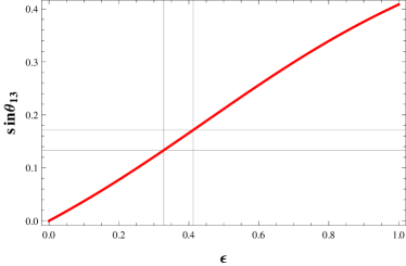
Figure 1: Plot of $\sin\theta_{13}$ against $\epsilon$. 3$\sigma$ range Forero:2014bxa of $\sin\theta_{13}$ (indicated by the horizontal lines) fixes $\epsilon$ in the range: 0.328-0.4125 (indicated by vertical lines).

With the above mentioned range of $\epsilon$, obtained from Fig. 1, the two other mixing angles $\theta_{12}$ and $\theta_{23}$ are found to be within the 3$\sigma$ range.

Expressions for the real and positive mass eigenvalues are obtained from Eq. (39-41) and can be written as

$$m_{1} = \alpha\frac{y}{k}\left|\sqrt{1-\epsilon+\epsilon^{2}}-k/y\right|,$$ (50)

$$m_{2} = \alpha\frac{y}{k}\left[1+\epsilon\right],$$ (51)

$$m_{3} = \alpha\frac{y}{k}\left[\sqrt{1-\epsilon+\epsilon^{2}}+k/y\right].$$ (52)

With the above mass eigenvalues, one can write the ratio of solar to atmospheric mass-squared differences as defined in Eq. (48) as:

$$r=\frac{3\epsilon\frac{y}{k}-\frac{k}{y}+2\sqrt{1-\epsilon+\epsilon^{2}}}{4\sqrt{1-\epsilon+\epsilon^{2}}}.$$ (53)

From Fig. 1, we have fixed $\epsilon$ range corresponding to 3$\sigma$ range of $\sin\theta_{13}$. Now, to satisfy $r=0.03$ Forero:2014bxa , we vary the ratio of the coupling constants, $y/k$, against $\epsilon$ using Eq. (48) and (50-52). The result is presented in Fig. 2.

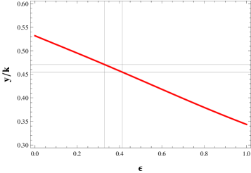
Figure 2: Contour plot of $r=0.03$ in $y/k-\epsilon$ plane. The vertical lines represent the allowed range for $\epsilon$ (0.328-0.4125) corresponding to 3$\sigma$ range of $\sin\theta_{13}$ which restricts the ratio $y/k$ between 0.471 to 0.455 indicated by horizontal lines.

The vertical patch there represents allowed region for $\epsilon$ fixed from Fig. 1 which determines the range of $y/k$ to be within 0.471-0.455. After obtaining $\epsilon$ and the ratio $y/k$, we can now find the factor $k/\Lambda$ (within $\alpha$) in order to satisfy the solar mass-squared difference $\Delta m^{2}_{\odot}=m^{2}_{2}-m^{2}_{1}=7.6\times 10^{-5}$ eV² Forero:2014bxa . Using Eq. (50) and (51) we find this factor to be

$$\frac{k}{\Lambda}=\frac{1}{v^{2}\epsilon\frac{y}{k}}\sqrt{\frac{\Delta m^{2}_{\odot}}{\left[3\epsilon-\left(\frac{k}{y}\right)^{2}+2\frac{k}{y}\sqrt{1+\epsilon^{2}-\epsilon}\right]}}.$$ (54)

Considering the 3$\sigma$ variation of $\sin\theta_{13}$, it falls within $1.97\times 10^{-15}$ GeV^-1 to $1.60\times 10^{-15}$ GeV^-1 with $v=246$ GeV.

  

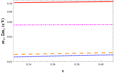
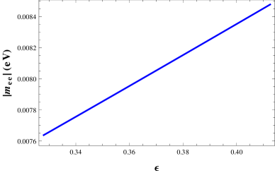
Figure 3: Left: Individual absolute neutrino masses ($m_{1}$- blue dotted line, $m_{2}$- orange dashed line, $m_{3}$- magenta dot-dashed line) and their sum (continuous red line) against $\epsilon$ (0.328-0.4125) corresponding to 3$\sigma$ range of $\sin\theta_{13}$. Right: Effective neutrino mass parameter (continuous blues line) against $\epsilon$ (0.328-0.4125) corresponding to 3$\sigma$ range of $\sin\theta_{13}$.

Parameters/Observable	Allowed Range
$\epsilon$	0.328-0.4125
$k/\Lambda$ (GeV-1)	$1.97\times 10^{-15}$ - $1.60\times 10^{-15}$
$\Sigma m_{i}$ (eV)	0.102 - 0.106
$|m_{ee}|$ (eV)	0.00764-0.00848

Table 2: Range of $\epsilon,k/\Lambda,\Sigma m_{i},|m_{ee}|$ for 3$\sigma$ range of $\sin\theta_{13}$ with $\phi_{ab}=\phi_{db}=0$.

Once we know about all parameters involved like $\epsilon,y/k,k/\Lambda$ with the specific choice of the phases (in this case $\phi_{ab}=\phi_{db}=0$), it is straightforward to determine absolute neutrino masses and effective neutrino mass parameter involved in neutrinoless double beta decay using

$$\left|m_{ee}\right|=\left|m_{1}^{2}c_{12}^{2}c_{13}^{2}+m_{2}^{2}s_{12}^{2}c_{13}^{2}e^{i\alpha_{21}}+m_{3}^{2}s_{13}^{2}e^{i(\alpha_{31}-2\delta)}\right|$$ (55)

as shown in Fig. 3. We also have listed the summary of the predictions of these quantities in Table 2.

3.2 Case B : $\phi_{db}=0$

Now we consider the case: $\phi_{db}=0$. Then the relations for $\theta_{\nu}$ and $\delta$ take the form

$$\tan{2\theta_{\nu}} = \frac{\sqrt{3}\epsilon}{(\epsilon-2\cos\phi_{ab})\cos\varphi}\,,$$ (56)

$$\tan\delta = -\frac{y}{k}\sin\phi_{ab}\,.$$ (57)

So from Eqs. (35, 56-57) and since $\tan\delta=\tan\varphi$, it is clear that unlike the Case A, here $\sin\theta_{13}$ depends not only on $\epsilon$ and $y/k$ but also on the phase present in the theory, $i.e.$ $\phi_{ab}$. Therefore there would exist a one to one correspondence between $\epsilon$ and $y/k$ in order to produce a specific value of $\sin\theta_{13}$ once a particular choice of $\delta$ has been made.

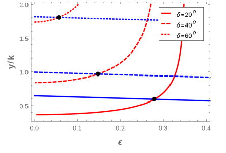
Figure 4: Contour plots for both $\sin\theta_{13}=0.1530$ (shown in red continuous, dashed and dotted lines) and $r=0.03$ (shown in blue continuous, dashed and dotted lines) for $\delta=20^{\circ},\delta=40^{\circ}$ and $\delta=60^{\circ}$ respectively in $\epsilon$-$y/k$ plane. Black dots on each intersection represents solution for $\epsilon$ and $y/k$ corresponding to each $\delta$ for $\phi_{db}=0$.

Now, with $\phi_{db}=0$, absolute neutrino masses given in Eq. (39-41) are reduced to

$$m_{1} = \alpha\frac{y}{k}\left[(P_{1}-\frac{k}{y})^{2}+Q_{1}^{2}\right]^{1/2},$$ (58)

$$m_{2} = \alpha\frac{y}{k}\left[1+\epsilon^{2}+2\epsilon\cos\phi_{ab}\right]^{1/2},$$ (59)

$$m_{3} = \alpha\frac{y}{k}\left[(P_{1}+\frac{k}{y})^{2}+Q_{1}^{2}\right]^{1/2},$$ (60)

with

$$P_{1}=\left[\frac{1}{2}(A_{1}+\sqrt{A_{1}^{2}+B_{1}^{2}})\right]^{1/2}\hskip 1.42271pt,\hskip 2.27626ptQ_{1}=\left[\frac{1}{2}(-A_{1}+\sqrt{A_{1}^{2}+B_{1}^{2}})\right]^{1/2},$$ (61)

$$A_{1}=\left(\epsilon^{2}+\cos 2\phi_{ab}-\epsilon\cos\phi_{ab}\right)\hskip 1.42271pt{\rm and}\hskip 2.27626ptB_{1}=\left(\sin 2\phi_{ab}-\epsilon\sin\phi_{ab}\right).$$ (62)

The ratio of solar to atmospheric neutrino mass-squared differences takes the form

$$r=\frac{1}{4P_{1}\frac{k}{y}}\left[(1+\epsilon^{2}+2\epsilon\cos\phi_{ab})-\left(P_{1}-\frac{k}{y}\right)^{2}-Q_{1}^{2}\right].$$ (63)

Clearly, one finds that $\epsilon$ and $y/k$ are the only parameters involved in both $\sin\theta_{13}$ and $r$ once $\delta$ values are taken as input. Therefore, those values of $\epsilon$ and $y/k$ are allowed which simultaneously satisfy data obtained for $\sin\theta_{13}$ and $r$ from neutrino oscillation experiments. Here we have considered the best fit values from Forero:2014bxa and drawn contour plots for $\sin\theta_{13}=0.1530$ and $r=0.03$. Intersection of these contours then represents solutions for $\epsilon$ and $y/k$. Note that $\delta=0$ case corresponds to the results obtained in Case A.

In Fig. 4, we have plotted typical contours obtained for $\sin\theta_{13}=0.1530$ (red lines) and $r=0.03$ (blue lines) for $\delta=20^{\circ},\delta=40^{\circ}$ and $\delta=60^{\circ}$ respectively in $\epsilon$-$y/k$ plane. The intersecting points are denoted by black dots and represent the solution points for $\epsilon$ and $y/k$. In Table 3 we have listed estimations for $\epsilon$ and $y/k$ for different $\delta$ values.

$\delta$	$\epsilon$	$y/k$	$k/\Lambda$ ($10^{-15}$ GeV-1)	$\Sigma m_{i}$ (eV)	$|m_{ee}|$ (eV)
$0^{\circ}$	0.372	0.463	1.756	0.1042	0.0222
$10^{\circ}$	0.343	0.496	1.910	0.1068	0.0236
$20^{\circ}$	0.279	0.592	2.361	0.1143	0.0274
$30^{\circ}$	0.209	0.745	3.140	0.1267	0.0331
$40^{\circ}$	0.147	0.966	4.405	0.1454	0.0409
$50^{\circ}$	0.096	1.288	6.610	0.1743	0.0516
$60^{\circ}$	0.056	1.803	11.10	0.2230	0.0682
$61^{\circ}$	0.053	1.873	11.80	0.2298	0.0704
$70^{\circ}$	0.026	2.798	23.22	0.3210	0.1002
$80^{\circ}$	0.007	5.743	85.42	0.6173	0.1952

Table 3: Estimated values of various parameters and observables satisfying neutrino oscillation data for different values of $\delta$ with $\phi_{db}=0$ .

Just like the previous case, after obtaining $\epsilon$ and $y/k$, we can find the factor $k/\Lambda$ using the fact that it has to produce correct solar mass-squared difference $\Delta m^{2}_{\odot}=m^{2}_{2}-m^{2}_{1}=7.6\times 10^{-5}$ eV² Forero:2014bxa . For this, we employ Eq. (58) and (59). All these findings are mentioned in Table 3 including sum of the absolute masses ($\Sigma m_{i}$) of all three light neutrinos and effective neutrino mass parameter involved in neutrinoless double beta decay ($|m_{ee}|$) for different considerations of leptonic CP phase $\delta$. In this analysis we observe that, for various values of $\delta$ between $0^{\circ}$ to $360^{\circ}$ there are certain points where same set of solutions for $\epsilon$ and $y/k$ are repeated ($\it e.g.$ solutions with $\delta$ is repeated for $|\pi-\delta|$). We should also employ the upper bound of sum of all three light neutrino masses ($\Sigma m_{i}<0.23$ eV) coming from cosmological observation by Planck planck . Once this is included, we note that some of the $\delta$ values need to be discarded as the corresponding sum of the masses exceeds 0.23 eV as seen from Table 3. We therefore conclude that the allowed values for $\delta$ are: between $0^{\circ}-61^{\circ}$ (and also $119^{\circ}-180^{\circ}$, $180^{\circ}-241^{\circ}$ and $299^{\circ}-360^{\circ}$).

3.3 Case C : $\phi_{ab}=0$

When $\phi_{ab}=0$, relations for $\theta_{\nu}$ and $\delta$ take the form

$$\tan{2\theta_{\nu}} = \frac{\sqrt{3}\epsilon\cos\phi_{db}}{(\epsilon\cos\phi_{db}-2)\cos\varphi},$$ (64)

$$\tan\delta = \frac{y}{k}\tan\phi_{ab}.$$ (65)

Here also $\sin\theta_{13}$ depends on $\epsilon,y/k$ and the phase involved $\phi_{db}$. The real and positive mass eigenvalues can be written as

$$m_{1} = \alpha\frac{y}{k}\left[(P_{2}-\frac{k}{y})^{2}+Q_{2}^{2}\right]^{1/2},$$ (66)

$$m_{2} = \alpha\frac{y}{k}\left[1+\epsilon^{2}+2\epsilon\cos\phi_{db}\right]^{1/2},$$ (67)

$$m_{3} = \alpha\frac{y}{k}\left[(P_{2}+\frac{k}{y})^{2}+Q_{2}^{2}\right]^{1/2},$$ (68)

with

$$P_{2}=\left[\frac{1}{2}(A_{2}+\sqrt{A_{2}^{2}+B_{2}^{2}})\right]^{1/2}\hskip 1.42271pt,\hskip 2.27626ptQ_{2}=\left[\frac{1}{2}(-A_{2}+\sqrt{A_{2}^{2}+B_{2}^{2}})\right]^{1/2},$$ (69)

where

$$A_{2}=\left(1+\epsilon^{2}\cos 2\phi_{db}-\epsilon\cos\phi_{db}\right)\hskip 1.42271pt{\rm and}\hskip 2.27626ptB_{2}=\left(\epsilon^{2}\sin 2\phi_{db}-\epsilon\sin\phi_{db}\right).$$ (70)

The ratio of solar to atmospheric neutrino mass-squared differences takes the form

$$r=\frac{y/k}{4P_{2}}\left[(1+\epsilon^{2}+2\epsilon\cos\phi_{db})-(P_{2}-k/y)^{2}-Q_{2}^{2}\right].$$ (71)

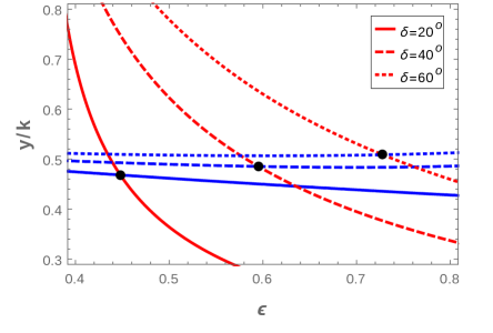
Figure 5: Contour plots for both $\sin\theta_{13}=0.1530$ (shown in red continuous, dashed and dotted lines) and $r=0.03$ (shown in blue continuous, dashed and dotted lines) for $\delta=20^{\circ},\delta=40^{\circ}$ and $\delta=60^{\circ}$ respectively in $\epsilon$-$y/k$ plane. Black dots on each intersection represents solution for $\epsilon$ and $y/k$ corresponding to each $\delta$ for $\phi_{ab}=0$.

We then scan the parameter space for $\epsilon$ and $y/k$ for various choices of $\delta$ so as to have $r=0.03$ and $\sin\theta_{13}=0.153$. In Fig. 5, we provide contour plots for $\sin\theta_{13}=0.1530$ (red lines) and $r=0.03$ (blue lines) for $\delta=20^{\circ},\delta=40^{\circ}$ and $\delta=60^{\circ}$. The intersection between $\sin\theta_{13}$ and $r$ contours indicate the simultaneous satisfaction of them. Hence the intersections are indicated by black dots with which a pair of $\epsilon,y/k$ are attached. Similar to the previous two cases, here we estimate the $k/\Lambda$ for each such pair of $\epsilon,y/k$ with a specific $\delta$. This in turn provide an estimate of $\Sigma m_{i}$ and effective mass parameter $|m_{ee}|$ depending on the choice of $\delta$. We provide these outcomes in Table 4.

$\delta$	$\epsilon$	$y/k$	$k/\Lambda$ ($10^{-15}$ GeV-1)	$\Sigma m_{i}$ (eV)	$|m_{ee}|$ (eV)
$0^{\circ}$	0.372	0.463	1.756	0.1042	0.0222
$10^{\circ}$	0.393	0.464	1.670	0.1048	0.0225
$20^{\circ}$	0.448	0.468	1.480	0.1065	0.0233
$30^{\circ}$	0.520	0.475	1.300	0.1093	0.0245
$40^{\circ}$	0.595	0.485	1.167	0.1128	0.0260
$50^{\circ}$	0.666	0.497	1.065	0.1162	0.0273
$60^{\circ}$	0.728	0.509	0.981	0.1182	0.0280
$70^{\circ}$	0.782	0.519	0.901	0.1179	0.0275
$80^{\circ}$	0.827	0.526	0.826	0.1152	0.0259

Table 4: Estimated values of various parameters and observables satisfying neutrino oscillation data for different values of $\delta$ with $\phi_{ab}=0$ .

3.4 Case D : $\phi_{ab}=\phi_{db}=\beta$

With $\phi_{ab}=\phi_{db}=\beta$, the mixing angle $\theta_{\nu}$ turns out to be function of $\epsilon$ only and is given by

$$\tan 2\theta_{\nu}=\frac{\sqrt{3}\epsilon}{\epsilon-2},$$ (72)

while $\tan\delta$ becomes zero. Note that the expressions for the mixing angle $\theta_{\nu}$ and $\delta$ are identical to the ones obtained in Case A. Therefore we use the constraint on $\epsilon$ obtained from Fig. 1 in order to satisfy $3\sigma$ allowed range of $\sin\theta_{13}$. However the expressions for real and positive mass eigenvalues involve the common phase $\beta$ and can be written as (following Eqs. (39-41))

$$m_{1} = \alpha\frac{y}{k}\left[\left(\sqrt{1-\epsilon+\epsilon^{2}}\cos\beta-\frac{k}{y}\right)^{2}+\left(\sqrt{1-\epsilon+\epsilon^{2}}\sin\beta\right)^{2}\right]^{1/2},$$ (73)

$$m_{2} = \alpha\frac{y}{k}\left[1+\epsilon\right],$$ (74)

$$m_{3} = \alpha\frac{y}{k}\left[\left(\sqrt{1-\epsilon+\epsilon^{2}}\cos\beta+\frac{k}{y}\right)^{2}+\left(\sqrt{1-\epsilon+\epsilon^{2}}\sin\beta\right)^{2}\right]^{1/2}.$$ (75)

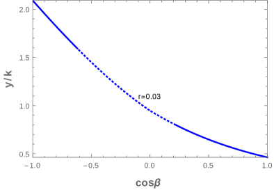
Figure 6: Contour plot for $r=0.03$ in the $y/k-\cos\beta$ plane for $\phi_{db}=\phi_{ab}=\beta$. The disallowed range of $y/k,\cos\beta$ is indicated by the dotted portion.

Then following our approach for finding the range of parameters which would satisfy the oscillation parameters obtained from experimental data, we define the ratio of solar to atmospheric mass-squared differences as defined in Eq. (48) as

$$r=\frac{3\epsilon\frac{y}{k}-\frac{k}{y}+2\cos\beta\sqrt{1-\epsilon+\epsilon^{2}}}{4|\cos\beta|\sqrt{1-\epsilon+\epsilon^{2}}}.$$ (76)

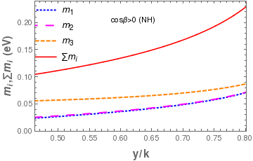
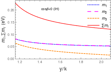
Figure 7: Absolute neutrino masses vs $y/k$ (blue dotted, magenta large-dashed, orange dashed and red continuous lines represent $m_{1}$, $m_{2}$, $m_{3}$ and $\sum m_{i}$ respectively). The left panel is for $\cos\beta>0$ and right panel is for $\cos\beta<0$.

From Fig. 1 we fix $\epsilon=0.372$ which would produce the best fit value of $\sin\theta_{13}$. Then, using the ratio of solar to atmospheric mass squared difference as given in Eq. (76), we can constrain $y/k$ and $\cos\beta$. Here we plot $r=0.03$ contour in the $y/k$-$\cos\beta$ plane as shown in Fig. 6. For $-1\leq\cos\beta\leq 1$. We observe that $y/k$ falls within the range: $0.463\leq\ y/k\leq 2.091$. Thus Fig. 6 establishes a correlation between $y/k$ and $\cos\beta$. Now to find absolute neutrino masses we need to obtain $k/\Lambda$ first. We can find $k/\Lambda$ from the best fit value for solar mass squared difference, $m^{2}_{2}-m^{2}_{1}=7.6\times 10^{-5}$ eV², and is given by

$$\left(\frac{k}{\Lambda}\right)^{2}=\frac{\Delta m^{2}_{\odot}}{4r(v^{2}\epsilon)^{2}y/k|\cos\beta|\sqrt{1+\epsilon^{2}-\epsilon}}.$$ (77)

We have used Eq. (73-75) to obtain the above equation. Once $\epsilon$ is fixed at 0.372 and following Fig. 6 we know $y/k$ and corresponding $\cos\beta$ (to have $r=0.03$), we can use Eq. (77) to have an estimate for $k/\Lambda$. Now by knowing $k/\Lambda$, we have plotted absolute masses for light neutrinos in Fig. 7 by using Eq. (73-75). Here the left (right) panel is for $\cos\beta>0(<0)$ and indicates normal (inverted) hierarchy for light neutrino masses. In Fig. 7, absolute neutrino masses $m_{1},m_{2},m_{3}$ and $\sum m_{i}$ are denoted by blue dotted, magenta large-dashed, orange dashed and red continuous lines respectively. Note that here we have plotted sum of the three absolute light neutrino masses consistent with the recent observation made by PLANCK, $i.e.$ $\sum m_{i}\leq 0.23$ eV planck . If we impose this constraint on the sum of absolute masses of the three light neutrinos, then the allowed region for $y/k$ gets further constrained. The dotted portion in Fig. 6 represents this excluded part. Therefore the allowed region for $y/k$ then turns out to be $0.463\leqslant y/k\leqslant 0.802$ for $\cos\beta>0$ (normal hierarchy) and $1.159\leqslant y/k\leqslant 2.091$ for $\cos\beta<0$ (inverted hierarchy). Finally in this case, the prediction for $|m_{ee}|$ found to be within $0.022\hskip 2.84544pt{\rm eV}<|m_{ee}|<0.039\hskip 2.84544pt{\rm eV}$ for normal hierarchy and $0.016\hskip 2.84544pt{\rm eV}<|m_{ee}|<0.035\hskip 2.84544pt{\rm eV}$ for inverted hierarchy.

4 Phenomenology of DM Sector

The dark sector consists of two vector-like fermions: a fermion doublet $\psi$ and a singlet $\chi$. The corresponding Lagrangian respecting the $U(1)$ and other discrete symmetries is provided in Eq. (18). At this stage we can remind ourselves about the minimality of the construction in terms of choice of constituents of the dark sector. Note that a vector-like singlet fermion alone can not have a coupling with the SM sector at the renormalizable level and thereby its relic density is expected to be over abundant (originated from interaction suppressed by the new physics scale $\Lambda$). On the contrary, a vector-like fermion doublet alone can have significant annihilation cross section from its gauge interaction with the SM sector and thereby we would expect the corresponding dark matter relic density to be under-abundant unless the DM mass is exorbitantly high. Hence we can naturally ask the question whether involvement of a singlet and a doublet vector-like fermions can lead to the dark matter relic density at an acceptable level. It then crucially depends on the mixing term between the singlet and the doublet fermions, $i.e.$ on $m_{D}=Yv$. We expect a rich phenomenology out of it particularly because the coupling $Y$ depends on the parameter $\epsilon$ through $Y=\epsilon^{n}$ where $\epsilon$ plays an important role in the neutrino physics as evident from our discussion in the previous section. We aim to restrict $n$ phenomenologically.

The electroweak phase transition along with the $U(1)$ breaking give rise to the following mass matrix in the basis $(\chi^{0},\psi^{0})$

$$\mathcal{M}=\begin{pmatrix}M_{\chi}&m_{D}\cr\\ m_{D}&M_{\psi}\,\end{pmatrix}.$$ (78)

We obtain mass eigenstates $\psi_{1}$ and $\psi_{2}$ with masses $M_{1}$ and $M_{2}$ respectively after diagonalization of the above matrix as

$$\psi_{1}=\cos\theta_{d}\chi^{0}+\sin\theta_{d}\psi^{0},$$

$$\psi_{2}=\cos\theta_{d}\psi^{0}-\sin\theta_{d}\chi^{0}\,,$$ (79)

where $\tan 2\theta_{d}=2m_{D}/{\left(M_{\psi}-M_{\chi}\right)}$. We will work in the regime where $m_{D}<<M_{\psi},M_{\chi}$. This choice would be argued soon. However this is not unnatural as the dark matter is expected to interact weakly. In this limit, the mass eigenvalues are found to be

$$M_{1}\approx M_{\chi}-\frac{m_{D}^{2}}{M_{\psi}-M_{\chi}},$$

$$M_{2}\approx M_{\psi}+\frac{m_{D}^{2}}{M_{\psi}-M_{\chi}}.$$ (80)

In this small mixing limit, we can write $M_{\psi}-M_{\chi}\simeq M_{2}-M_{1}=\Delta M$. Therefore the mixing angle $\theta_{d}$ can be approximately represented by

$$\sin 2\theta_{d}\simeq\frac{2Yv}{\Delta M}\,.$$ (81)

Then as evident from Eqs. (79), $\psi_{1}$ is dominantly the singlet having a small admixture with the doublet. We assume it to be the lightest between the two ($i.e.~{}M_{1}<M_{2}$) and forms the DM component of the universe. In the physical spectrum, we also have a charged fermion $\psi^{+}(\psi^{-})$ with mass $M^{+}(M^{-})=M_{1}\sin^{2}\theta_{d}+M_{2}\cos^{2}\theta_{d}$. In the limit $\theta_{d}\to 0$, $M^{\pm}=M_{2}=M_{\psi}$. In this section, we will discuss the relic density of dark matter as a function of $Y$. Although $Y$ represents Yukawa coupling of the DM with SM Higgs, in presence of a singlet and doublet fermions, $Y$ is also a function of the mixing angle $\sin\theta_{d}$ as well as the mass splitting ($\Delta M$ as in Eq. (81)) which crucially controls DM phenomenology as we demonstrate in the following discussion.

Figure 8: Dominant Annihilation processes to Higgs and Gauge boson final states.

Note that $\psi_{0}$ being the gauge doublet, it carries the gauge interactions and hence, the physical mass eigenstates including the DM have the following interaction with $Z,W$ bosons as :

$$\frac{g}{\sqrt{2}}\overline{\psi_{0}}\gamma^{\mu}W_{\mu}^{+}\psi^{-}+{\rm h.c.}\to\frac{g\sin\theta_{d}}{\sqrt{2}}\overline{\psi_{1}}\gamma^{\mu}W_{\mu}^{+}\psi^{-}+\frac{g\cos\theta_{d}}{\sqrt{2}}\overline{\psi_{2}}\gamma^{\mu}W_{\mu}^{+}\psi^{-}+{\rm h.c.}\,,$$ (82)

$$\frac{g}{2\cos\theta_{w}}\overline{\psi_{0}}\gamma^{\mu}Z_{\mu}\psi_{0} \to\frac{g}{2\cos\theta_{w}}\left(\sin^{2}\theta_{d}\overline{\psi_{1}}\gamma^{\mu}Z_{\mu}\psi_{1}+\sin\theta_{d}\cos\theta_{d}(\overline{\psi_{1}}\gamma^{\mu}Z_{\mu}\psi_{2}+\overline{\psi_{2}}\gamma^{\mu}Z_{\mu}\psi_{1})\right.$$

$$~{}~{}~{}~{}~{}~{}~{}~{}~{}~{}~{}~{}~{}~{}~{}~{}~{}~{}~{}~{}~{}~{}~{}~{}~{}~{}~{}~{}~{}~{}~{}~{}~{}~{}~{}~{}~{}~{}~{}~{}~{}~{}~{}~{}\left.+\cos^{2}\theta_{d}\overline{\psi_{2}}\gamma^{\mu}Z_{\mu}\psi_{2}\right)\,.$$ (83)

The relic density of the dark matter ($\psi_{1}$) is mainly dictated by annihilations through (i) $\overline{\psi_{1}}\psi_{1}\to W^{+}W^{-},ZZ$ through $SU(2)_{L}$ gauge coupling and (ii) $\overline{\psi_{1}}\psi_{1}\to hh$ through Yukawa coupling introduced in Eq. (17). The relevant processes

Figure 9: Dominant Co-Annihilations $\psi_{1}\bar{\psi_{2}}$ to Higgs and Gauge boson final states.

are indicated in Fig. 8. The other possible channels are mainly co-annihilation of $\psi_{1}$ with $\psi_{2}$ (see Fig. 9), $\psi_{1}$ with $\psi^{\pm}$ (see Fig. 10) and annihilations of $\psi^{\pm}$ (see Fig. 11) which would dominantly contribute to relic density in a large region of parameter space Bhattacharya:2015qpa ; griest ; Cynolter:2008ea ; Cohen:2011ec ; Cheung:2013dua as can be seen once we proceed further. At this stage we can argue on our choice of making $\theta_{d}$ small, or in other words why the mixing with doublet is necessary to be small for the model to provide a DM with viable relic density. This is because the larger is the doublet content in DM $\psi_{1}$, the annihilation goes up significantly in particular through $\psi_{1}\overline{\psi_{1}}\to W^{+}W^{-}$ through $Z$ and hence yielding a very small relic density. So in the small mixing limit, $\psi_{2}$ is dominantly a doublet having a mixture of minor singlet component. This implies that $\psi_{2}$ mass is required to be larger than 45 GeV in order not to be in conflict with the invisible $Z$-boson decay width.

Figure 10: Dominant Co-Annihilation $\bar{\psi_{1}}\psi^{-}$ to Higgs and gauge boson final states.

The relic density of the $\psi_{1}$ DM with mass $M_{1}$ can be given by griest

$$\Omega_{\psi_{1}}h^{2}=\frac{1.09\times 10^{9}\rm~{}GeV^{-1}}{g_{\star}^{1/2}M_{PL}}\frac{1}{J(x_{f})}\,,$$ (84)

where $J(x_{f})$ is given by

$$J(x_{f})=\int_{x_{f}}^{\infty}\frac{\langle\sigma|v|\rangle_{eff}}{x^{2}}\hskip 5.69046ptdx\,.$$ (85)

Figure 11: Dominant Co-Annihilation processes of ${\psi^{+}}\psi^{-}\rightarrow$ SM particles where $f$ represents SM fermions.

Here $\langle\sigma|v|\rangle_{eff}$ is the thermal average of dark matter annihilation cross sections including contributions from co-annihilations as follows:

$$\begin{split}\langle\sigma|v|\rangle_{eff}=&\frac{g_{1}^{2}}{g_{eff}^{2}}\sigma(\overline{\psi_{1}}\psi_{1})+2\frac{g_{1}g_{2}}{g_{eff}^{2}}\sigma(\overline{\psi_{1}}\psi_{2})(1+\Delta)^{3/2}exp(-x\Delta)\\ &+2\frac{g_{1}g_{3}}{g_{eff}^{2}}\sigma(\overline{\psi_{1}}\psi^{-})(1+\Delta)^{3/2}exp(-x\Delta)\\ &+2\frac{g_{2}g_{3}}{g_{eff}^{2}}\sigma(\overline{\psi_{2}}\psi^{-})(1+\Delta)^{3}exp(-2x\Delta)+\frac{g_{2}g_{2}}{g_{eff}^{2}}\sigma(\overline{\psi_{2}}\psi_{2})(1+\Delta)^{3}exp(-2x\Delta)\\ &+\frac{g_{3}g_{3}}{g_{eff}^{2}}\sigma(\psi^{+}\psi^{-})(1+\Delta)^{3}exp(-2x\Delta)\,.\end{split}$$ (86)

In the above equation $g_{1}$,$g_{2}$ and $g_{3}$ are the spin degrees of freedom for $\psi_{1}$, $\psi_{2}$ and $\psi^{-}$ respectively. Since these are spin half particles, all $g$’s are 2. The freeze-out of $\psi_{1}$ is parameterised by $x_{f}=\frac{M_{1}}{T_{f}}$, where $T_{f}$ is the freeze out temperature. $\Delta$ depicts the mass splitting ratio as $\Delta=\frac{M_{2}-M_{1}}{M_{1}}=\frac{\Delta M}{M_{1}}$, where $M_{2}$ stands for the mass of both $\psi_{2}$ and $\psi^{\pm}$. The effective degrees of freedom $g_{eff}$ in Eq. (86) is given by

$$g_{eff}=g1+g_{2}(1+\Delta)^{3/2}exp(-x\Delta)+g_{3}(1+\Delta)^{3/2}exp(-x\Delta)\,.$$ (87)

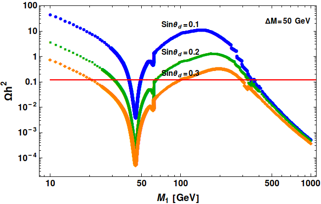
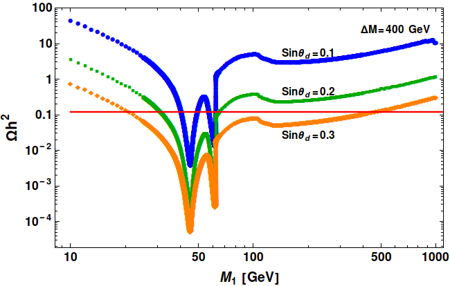
Figure 12: Relic density vs DM mass $M_{1}$ (in GeV) for different choices of $\sin\theta_{d}=\{0.1,0.2,0.3\}$ with $\Delta M=50$ GeV [left] (corresponding to $Y=\{0.02,0.04,0.058\}$ with blue, green, orange respectively) and $\Delta M=400$ GeV [right] (corresponding to $Y=\{0.16,0.32,0.46\}$ with Blue, Green, Orange respectively). Horizontal lines define the correct relic density.

As it turns out from the above discussion, the dark-sector phenomenology in our set-up is mainly dictated by three parameters $\sin\theta_{d},M_{1}$ and $\Delta M$. However we will keep on changing $\sin\theta_{d}$ and/or $\Delta M$ dependence with $Y$ wherever required using Eq.(81). In the following we use the code MicrOmegas Belanger:2008sj to find the allowed region of correct relic abundance for our DM candidate $\psi_{1}$ satisfying PLANCK constraints planck ; Ade:2015xua ,

$$0.1175\leq\Omega_{\rm DM}h^{2}\leq 0.1219\,.$$ (88)

In Fig. 12 we plot relic density versus DM mass $M_{1}$ for different choices of $\sin\theta_{d}=0.1,0.2$ and 0.3 (represented by blue, green and orange dotted lines respectively) while keeping the mass difference $\Delta M$ fixed at 50 GeV in the left panel and at $\Delta M=400$ GeV in the right panel. The choice of various $\sin\theta_{d}$ can be translated into different values of $Y$ as well, through Eq. (81) since $\Delta M$ is kept fixed. Then it is equivalent to say that the blue, green and orange dotted lines in the left panel ($\Delta M$ = 50 GeV) represent $Y$= 0.02, 0.04, 0.058 respectively. In a similar way, the blue, green and orange dotted lines in the right panel ($\Delta M$ = 400 GeV) represent $Y$ = 0.16, 0.32, 0.46 respectively. We infer that as the mixing increases or in other words $Y$ increases ($\Delta M$ is fixed), the doublet component starts to dominate (see Eq. (81)) and hence give larger cross-section which leads to a smaller DM abundance for a particular $M_{1}$. The second important point to note is the presence of $Z$ resonance at $M_{1}=M_{Z}/2\sim 45$ GeV and a Higgs resonance at $M_{1}=M_{H}/2\sim 63$ GeV where relic density drops sharply due to increase in annihilation cross-section. We can also see that with larger $\Delta M$, $i.e.$ with larger $Y$ (as $\sin\theta_{d}$ is fixed) in the right hand side, the Higgs resonance is more prominent for obvious reasons. Relic density for these chosen parameters are satisfied across the $Z$ resonance window and $H$ resonance window (more prominent for larger $\Delta M$ on the right panel). For small $\Delta M=50$ GeV (left panel of Fig. 12), relic density drops beyond DM mass of 300 GeV. This is due to co-annihilation channels start contributing $\overline{\psi_{2}}\psi_{1}\to SM$ or $\overline{\psi^{+}}\psi_{1}\to SM$ and we find that the relic density is satisfied for DM mass $\sim$ 400 GeV. This is however not seen in the right panel where we have larger $\Delta M$. This is because with the large mass gap, co-annihilation doesn’t contribute significantly due to Boltzmann suppression for DM masses upto TeV. That is why with larger $\Delta M$ (right panel of Fig. 12), there is no point for DM mass beyond 100 GeV associated with smaller $\sin\theta_{d}$ values like 0.1, 0.2, where relic density constraint is satisfied. With larger $\sin\theta_{d}=0.3$ one can satisfy relic density without the aid of co-annihilation for $M_{1}\sim$ 500 GeV. We also note a small drop in relic density on the right panel in particular, when $WW$ and $ZZ$ channels open up for annihilation.

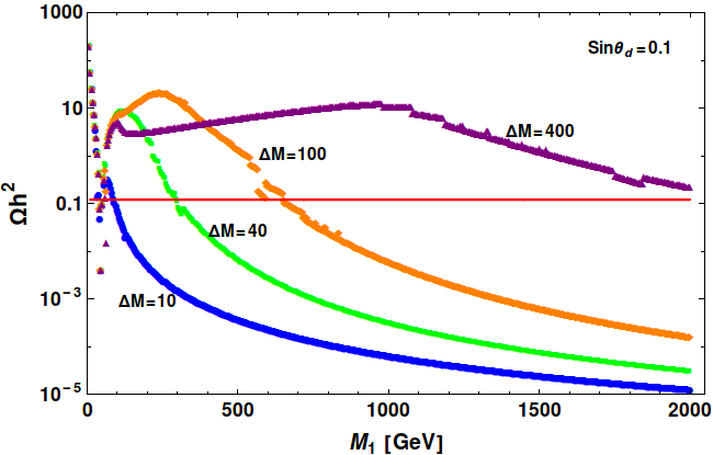
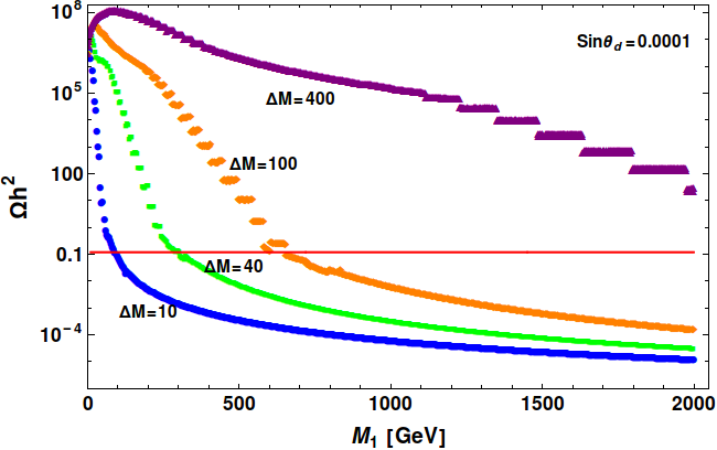
Figure 13: Left: $\Omega h^{2}$ versus Dark matter mass $M_{1}$ (in GeV) for $\sin\theta_{d}=0.1$ with different choices of $\Delta M=\{10,40,100,400\}$ GeV described by $\{$ blue, green, orange, purple respectively$\}$. Right: Same as left panel but with different $\sin\theta_{d}=0.0001$. Horizontal lines indicate correct relic density.

In order to show the effect of co-annihilations more closely, we draw Fig. 13, where one can see the $\Delta M$ dependency on relic density for a specific choice of mixing angle. In the left panel we choose $\sin\theta_{d}=0.1$ and that in the right panel for $\sin\theta_{d}=0.0001$. The slices with constant $\Delta M$ is shown for $\Delta M=\{10,40,100,400\}~{}{\rm GeV}$ in blue, green, orange, purple lines respectively. We note here, that with larger $\Delta M$, annihilation cross-section increases due to enhancement in Yukawa coupling ($Y\propto\Delta M$ as $\sin\theta_{d}$ is fixed). However, co-annihilation decreases due to increase in $\Delta M$ as $\sigma\propto e^{-\Delta M/M_{1}}$ specifically for a particular DM mass. Hence the larger is $\Delta M$ the smaller is co-annihilation and the larger is the relic density. This is clearly visible in both the panels of Fig. 13. In particular, when $\sin\theta_{d}$ is small, the effect of co-annihilation is pronounced as contribution from annihilation cross section is less dominant. This is the case shown in the right panel of Fig. 13. Hence the bigger is $\Delta M$, the larger is the required DM mass to satisfy relic density for a given mixing angle $\sin\theta_{d}$. This is evident from the plot with $\Delta M=400$ GeV.

For extremely small mixing angle, say $\sin\theta_{d}=0.0001$ (shown on the right panel of Fig. 13), the annihilation of $\bar{\psi}_{1}\psi_{1},\bar{\psi}_{1}\psi_{2}\to SM$ particles are highly suppressed. As a result the dominant contribution to relic density arises from $\psi_{2}\psi^{\pm},\psi^{+}\psi^{-}\to$ SM particles. This is an interesting consequence of our model. In this case we get a lower limit of the singlet-doublet mixing angle by assuming that the $\psi_{2},\psi^{\pm}$ particles decay to $\psi_{1}$ before the latter freezes out from the thermal bath Bhattacharya:2015qpa . If the mass splitting between $\psi^{-}$ and $\psi_{1}$ is larger than $W^{\pm}$-boson mass, then $\psi^{-}$ decay preferably occurs through the two body process: $\psi^{-}\to\psi_{1}+W^{-}$. However, if the mass splitting between $\psi^{-}$ and $\psi_{1}$ is less than $W^{\pm}$ boson mass, then $\psi^{-}$ decays through three body process, say $\psi^{-}\to\psi_{1}\ell^{-}\overline{\nu_{\ell}}$. For the latter case, we get a stronger lower bound on the mixing angle than for two body decay. For the above mentioned channel, the three body decay width of $\psi^{-}$ is given by Bhattacharya:2015qpa :

$$\Gamma=\frac{G_{F}^{2}sin^{2}\theta_{d}}{24\pi^{3}}M_{2}^{5}I$$ (89)

where $G_{F}$ is the Fermi coupling constant and $I$ is given as:

$$I=\frac{1}{4}\lambda^{1/2}(1,a^{2},b^{2})F_{1}(a,b)+6F_{2}(a,b)\ln\left(\frac{2a}{1+a^{2}-b^{2}-\lambda^{1/2}(1,a^{2},b^{2})}\right)\,.$$ (90)

In the above Equation $F_{1}(a,b)$ and $F_{2}(a,b)$ are two polynomials of $a=M_{1}/M_{2}$ and $b=m_{\ell}/M_{2}$, where $m_{\ell}$ is the charged lepton mass. Up to ${\cal O}(b^{2})$, these two polynomials are given by

$$F_{1}(a,b) = \left(a^{6}-2a^{5}-7a^{4}(1+b^{2})+10a^{3}(b^{2}-2)+a^{2}(12b^{2}-7)+(3b^{2}-1)\right)$$

$$F_{2}(a,b) = \left(a^{5}+a^{4}+a^{3}(1-2b^{2})\right)\,.$$ (91)

In Eq. (90), $\lambda^{1/2}=\sqrt{1+a^{4}+b^{4}-2a^{2}-2b^{2}-2a^{2}b^{2}}$ defines the phase space. In the limit $b=m_{\ell}/M_{2}\to 1-a=\Delta M/M_{2}$, $\lambda^{1/2}$ goes to zero and hence $I\to 0$. The life time of $\psi^{-}$ is then given by $\tau\equiv\Gamma^{-1}$. Now to compare the life time of $\psi^{-}$ with DM freeze out epoch, we assume that the freeze out temperature of DM is $T_{f}=M_{1}/20$. Since the DM freezes out during radiation dominated era, the corresponding time of DM freeze-out is given by :

$$t_{f}=0.301g_{\star}^{-1/2}\frac{m_{\rm pl}}{T_{f}^{2}}\,,$$ (92)

where $g_{\star}$ is the effective massless degrees of freedom at a temperature $T_{f}$ and $m_{\rm pl}$ is the Planck mass. Demanding that $\psi^{-}$ should decay before the DM freezes out (i.e. $\tau\lesssim t$) we get

$$\sin\theta_{d}\gtrsim 1.1789\times 10^{-5}\,\,\left(\frac{1.375\times 10^{-5}}{I}\right)^{1/2}\left(\frac{200\rm GeV}{M_{2}}\right)^{5/2}\left(\frac{g_{\star}}{106.75}\right)^{1/4}\left(\frac{M_{1}}{180\rm GeV}\right)\,.$$ (93)

Notice that the lower bound on the mixing angle depends on the mass of $\psi^{-}$ and $\psi_{1}$.

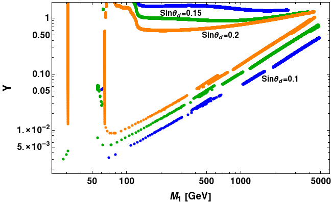
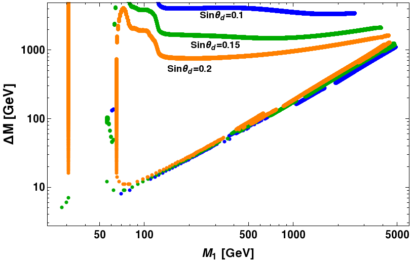
Figure 14: Left: $Y$ versus $M_{1}$ (in GeV) for correct relic density (Eq. 88). $\sin\theta_{d}=0.1,~{}0.2,~{}0.15$ (blue, green and orange respectively) has been chosen, while $\Delta M$ vary arbitrarily. Right: Same plot in $M_{1}-\Delta M$ plane.

In Fig. 14 (left), we plot $Y$ versus $M_{1}$ to produce correct relic density with $\sin\theta_{d}=\{0.1,~{}0.15,~{}0.2\}$ (blue, orange, green respectively). In order to be consistent with Eq. (81), $\Delta M$ has to be adjusted accordingly. It points out a relatively wide DM mass range satisfy the relic density constraint. Main features that emerge out of this figure are as follows: (i) Firstly, there exist a lower DM mass region where $Z$ and $H$ resonances occur. Relic density is easily satisfied in this region for all possible moderate choices of $\sin\theta_{d}$, independent of $Y$ or $\Delta M$ as is seen on the left hand side vertical lines (in both the plots). For large $\sin\theta_{d}$ this is more prominent as both $Z$ and $H$ mediation is enhanced with larger mixing. (ii) The other point is to note that there are two regions for each $\sin\theta_{d}$ value which satisfy relic density; one at the below, where $Y$ (on the left) and $\Delta M$ (on the right panel) increase with larger DM mass to satisfy relic density. This region is dominantly contributed from co-annihilations as the small $Y$ is not enough to produce annihilations required for relic density. While there is a second region with larger $Y$ (on left) and larger $\Delta M$ (on right), more insensitive to DM mass, where relic density is satisfied by appropriate annihilation cross-section, not aided by co-annihilations. Both of these regions (annihilation and co-annihilation domination) meet at some large DM mass $\sim$ 5000 GeV, more clearly visible from the right panel plot. Points above the ‘correct annihilation lines’ (for specific $\sin\theta_{d}$) provide more than required annihilation and hence those are under abundant regions. Similarly just below those, the annihilation will not be enough to produce correct density and hence are over abundant regions. Points below the correct co-annihilation regions produce more co-annihilations than required and hence depict under abundant regions.

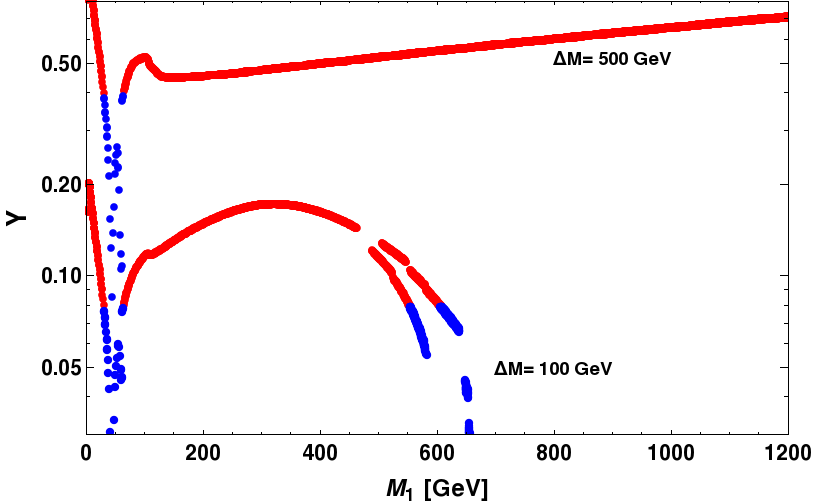
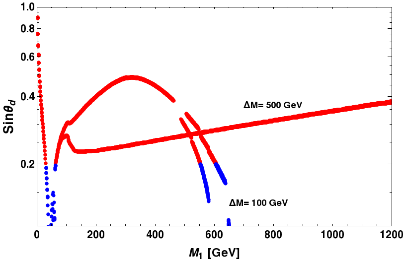
Figure 15: Left: $Y$ versus $M_{1}$ (in GeV) for correct relic density (within the range given by Eq. (88)) with fixed $\Delta M$ at 100, 500 GeV, while $\sin\theta_{d}$ is allowed to vary. Right: Same plot in $M_{1}-\sin\theta_{d}$ plane. In both panels, blue dots are the allowed points for small $\sin\theta_{d}$ to satisfy the $Y,~{}\Delta M$ abundance via Eq. (81).

The other possible correlation in this model for correct relic density can be drawn between DM mass ($M_{1}$) and the mixing angle ($\sin\theta_{d}$) for fixed $\Delta M$. This is shown in Fig. 15 both in $M_{1}-Y$ plane (on the left) or in $M_{1}-\sin\theta_{d}$ plane (on the right). For illustration, we choose two widely different values of mass difference: $\Delta M=100$ GeV and $\Delta M=500$ GeV. This is clearly understood that with larger $\Delta M$, a larger $Y$ is favored for a specific DM mass in order to satisfy the correct relic abundance. With $\Delta M$ = 100 GeV we also note that $Y$ drops substantially around $M_{1}\sim$ 500 GeV. This is because around this value, co-annihilation process starts contributing and hence it requires a further drop in $Y$ (in terms of mixing angle $\theta_{d}$) to obtain right relic density which is clearly visible in the right side of Fig. 15 as well. Here we would like to draw the attention that the right relic density line has a split when co-annihilation starts dominating. This is due to the fact that there are two different co-annihilations that occur here with $\psi_{2}$ and $\psi^{\pm}$. There exist a slight mass difference between these particles and the DM mass is adjusted to either of them to effectively co-annihilate and produce right relic density. For $\Delta M$ = 500 GeV, this phenomena of co-annihilation occurs at a very large DM mass and can’t be seen from the plot. Resonance drops both in $Y-M_{1}$ and $\sin\theta_{d}-M_{1}$ plots can be observed for $M_{1}\sim M_{H}/2$ and $M_{1}\sim M_{Z}/2$. We also note that beyond $\sin\theta_{d}\geq 0.2$ as shown by the red points in Fig. 15 break small $\theta_{d}$ limit as has been assumed in Eq. (81) and hence discarded within this approximation.

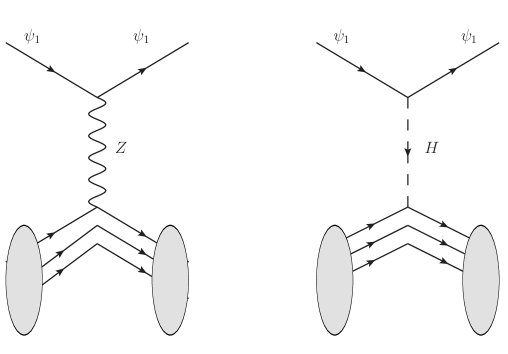
Figure 16: Feynman diagrams for DM to interact with Nucleon.

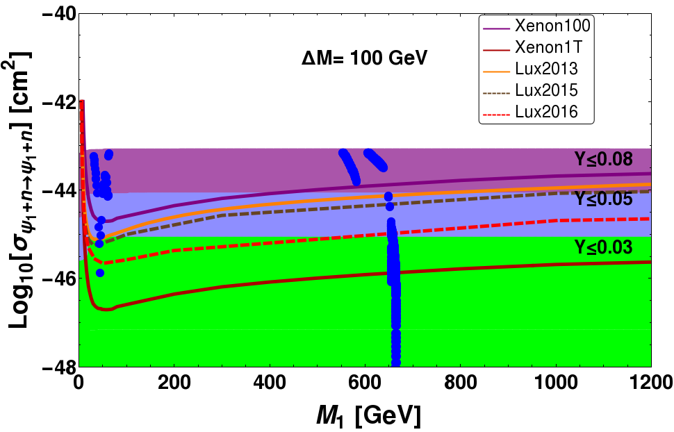
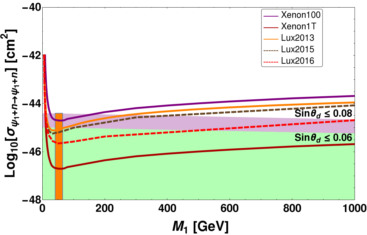
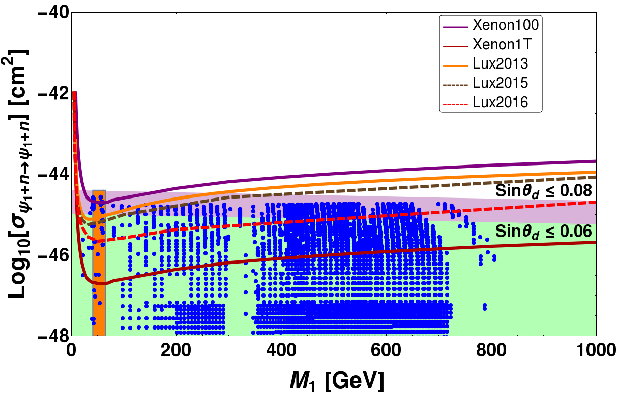
Figure 17: Spin independent direct search cross-section as a function of DM mass. Upper Left Panel: Different Y ranges are indicated $Y:\{0.001-0.03\}$ (green), $Y:\{0.03-0.05\}$ (blue) and $Y:\{0.05-0.08\}$ (purple). $\Delta M=100$ GeV is used for the scan. Upper Right Panel: Same as left, additional blue dots represent points which satisfy relic density constraint. Lower left panel: Allowed ranges of $\sin\theta_{d}\leq 0.06,0.08$ (light green and lilac regions respectively) are shown. Here $\Delta M$ varies arbitrarily upto 1.1 TeV. Lower right panel is same as the lower left panel having blue dots representative of points which satisfy relic density constraint. The resonance region is separately indicated in orange. Constraints from Xenon100, Lux 2013, 2015, 2016 data and predictions of Xenon1T are presented.

Non-observation of DMs in direct search experiments tend to put a stringent bound on WIMP DM parameter space. Direct search interactions for $\psi_{1}$ has two different channels, through $Z$ and $H$ mediation as shown in Fig. 16, where the one through $Z$ mediation dominates over $H$ mediated interaction because of $SU(2)$ gauge coupling. The cross-section per nucleon for $Z$ mediation is given by Goodman:1984dc ; Essig:2007az

$$\sigma_{\rm SI}^{Z}=\frac{1}{\pi A^{2}}\mu_{r}^{2}|\mathcal{M}|^{2}$$ (94)

where $\mu_{r}=M_{1}m_{n}/(M_{1}+m_{n})\approx m_{n}$ is the reduced mass, $m_{n}$ is the mass of nucleon (proton or neutron), $A$ is the mass number of the target nucleus and $\mathcal{M}$ is the amplitude for $Z$-mediated DM-nucleon cross-section

$$\mathcal{M}=\sqrt{2}G_{F}[Z(f_{p}/f_{n})+(A-Z)]f_{n}\sin^{2}\theta_{d}\,,$$ (95)

$f_{p}$ and $f_{n}$ are the interaction strengths of DM with proton and neutron respectively and $Z$ is the atomic number of the target nucleus. Using $f_{n}\simeq 1/3$  Koch:1982pu ; Gasser:1990ap ; Pavan:2001wz ; Bottino:2008mf , we obtain direct search cross-section per nucleon to be

$$\sigma_{\rm SI}^{Z}\simeq 3.75\times 10^{-39}{\rm cm}^{2}\sin^{4}\theta_{d}\,.$$ (96)

Higgs mediated cross-section depends on can be written as

$$\sigma_{\rm SI}^{h}=\frac{1}{\pi A^{2}}\mu_{r}^{2}\left[Zf_{p}+(A-Z)f_{n}\right]^{2}$$ (97)

where the effective interaction strengths of DM with proton and neutron are given by:

$$f_{p,n}=\sum_{q=u,d,s}f_{Tq}^{(p.n)}\alpha_{q}\frac{m_{(p,n)}}{m_{q}}+\frac{2}{27}f_{TG}^{(p,n)}\sum_{q=c,t,b}\alpha_{q}\frac{m_{p.n}}{m_{q}}$$ (98)

with

$$\alpha_{q}=\frac{Y\sin 2\theta_{d}}{M_{h}^{2}}\left(\frac{m_{q}}{v}\right)\,.$$ (99)

We compute the direct search cross-section with both diagrams using MicrOmegas Belanger:2008sj . It turns out that the most stringent constraint on the model and hence on the portal coupling $Y$ ($\lesssim\sin 2\theta_{d}\Delta M/(2v))$ comes from the direct search of DM from updated LUX data Akerib:2016vxi as demonstrated in Fig. 17. We show the correct region of direct search allowed parameter space in two ways: in upper panel we choose a specific $\Delta M$ and vary $\sin\theta_{d}$ to evaluate spin independent direct search cross-section and show the constraints in terms of $Y$. On the upper right panel, we also show the relic density allowed points through blue dots for this particular choice of $\Delta M$. In the bottom panel of Fig. 17, instead of choosing a specific $\Delta M$, we vary it arbitrarily upto 1.1 TeV and point out the direct search constraints in terms of mixing angle $\sin\theta_{d}$. On the right bottom panel, we also show the relic density allowed points through blue dots. Restricting direct search cross-section to experimental limit actually puts a stringent bound on mixing angle $\sin\theta_{d}$ to tame Z-mediated diagram in particular. We see that the bound from LUX, constraints the coupling: $Y\sim 0.03$ for DM masses $\gtrsim 600$ GeV (green regions in the upper panel of Fig. 17). The Yukawa coupling needs to be even smaller for small DM mass for example, $M_{1}\simeq 200$ GeV. The resonance region is exempted from this constraint for obvious reasons. The annihilation cross-section is enhanced due to s-channel contribution and to tame it to right relic density, one needs much smaller values of mixing angle, which sharply drops the direct search cross-section. Though large couplings are allowed by correct relic density, they are highly disfavored by the direct DM search at terrestrial experiments. From the top right figure, we also see that correct relic density points for a specific $\Delta M$ lies in the vicinity of a specific DM mass $\sim$ 700 GeV where co-annihilation plays the crucial role for correct relic density and that doesn’t contribute to direct search cross-section at all, so that the blue points yield very small direct search cross-sections. This can easily be extended for other choices of $\Delta M$, where there exist a specific DM mass at which co-annihilation plays a crucial role to yield right relic density, which doesn’t contribute to direct search and thus can have very small direct search cross-section as is seen from the right bottom figure. Note also that direct search constraints are less dependent on $\Delta M$ as to the mixing angle, which plays otherwise a crucial role in the relic abundance of DM. In bottom panel, we show the parameter space satisfied by relic density constraint for $\sin\theta_{d}\leq 0.08,0.06$ (lilac and green regions respectively) to direct search constraints. The direct search tightly constraints the mixing angle to $\sin\theta_{d}\leq 0.08$, allowing DM masses as heavy as 900 GeV. Tighter constraint in mixing angle, for example, $\sin\theta_{d}\leq 0.06$, allows smaller DM mass $\geq 500$ GeV as can be seen from the cross-over of LUX constraint with relic density allowed parameter space.

In summary, the dark sector phenomenology with the inclusion of vector-like fermions provides a simple extension to SM, with a rich phenomenology with a large region of allowed parameter space from relic density constraints. Direct search on the other hand constrains the mixing to a small value $\leq 0.08$, allowing co-annihilation to play a dominant part to keep the model alive. We will focus on the correlations to non-zero $\theta_{13}$ and DM in the following section with the results obtained from above analysis. Note that the $U(1)$ symmetry being global, its spontaneous breaking would lead to potentially dangerous Goldstone boson ($G$ = Im$\phi$). The problem however can be evaded by gauging the symmetry. Additionally if we assume the corresponding gauge boson to be sufficiently heavy, its existence will not modify our results of the dark matter phenomenology. Another way out is to provide tiny mass to the Goldstone by introducing an explicit symmetry breaking term in the Lagrangian. In this case however the most significant coupling of the Goldstone with Higgs appears through $\lambda_{12}\phi^{\dagger}\phi H^{\dagger}H$ coupling. Hence it contributes (considering $m_{G}\ll m_{h}/2$) to the invisible decay of the SM Higgs boson Joshipura:1992hp , $\Gamma_{h\rightarrow G~{}G}\sim\frac{1}{32\pi}[m_{h}^{3}/\langle\phi\rangle]\sin^{2}\alpha$, where $\alpha$ signifies the mixing between the states $(H,\phi)$ and the physical Higgs fields $(h,H^{\prime})$ resulting ($H^{\prime}$ is the heavy Higgs) from non-zero $\lambda_{12}$. In the limit of $\lambda_{12}$ to zero, $\alpha$ vanishes. Using the present limit on the branching ratio of Higgs invisible decay Aad:2015txa ; Khachatryan:2016whc , the coupling $\lambda_{12}$ (involved in the definition of mixing angle $\alpha$) is expected to be small ($\ll 1$). If we assume a very small value of $\lambda_{12},~{}\sim 10^{-8}$ or even smaller, then it can be shown that the Goldstone can never be in thermal equilibrium Burgess:2000yq and hence they can not contribute to the primordial abundance through freeze out mechanism and we may basically ignore its presence for our purpose.

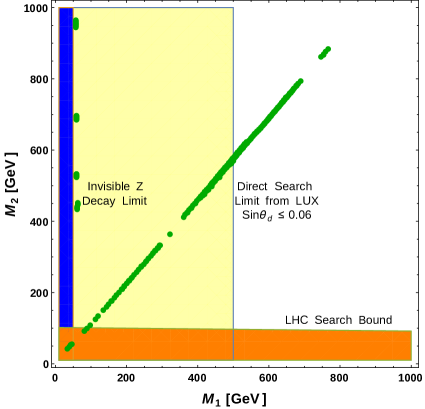
Figure 18: Summary of all constraints in $M_{1}-M_{2}$ parameter space from relic density with $\sin\theta_{d}=0.06$ (green dots), direct search (Yellow region is forbidden by updated LUX with $\sin\theta_{d}\sim 0.06$), invisible Z-decay (blue region is forbidden) and collider (LHC) search limit (orange region is disallowed with an over estimation for $\sin\theta_{d}=0.1$).

We can now put together all the constraints for a specific choice of $\sin\theta_{d}=0.06$ into the plane of $M_{1}-M_{2}$ to show the allowed parameter space of the model. This is what we have done in Fig. 18 following

$$\rm{Inv~{}Z~{}decay}:M_{1}<\frac{M_{z}}{2}\sim 45~{}GeV \to\sin\theta_{d}\lesssim 0.00125$$

$$\rm{Inv~{}H~{}decay}:M_{1}<\frac{M_{h}}{2}\sim 63~{}GeV \to\sin\theta_{d}\lesssim 0.1$$

$$\rm{Relic~{}Density}:M_{2}\lesssim M_{1}+100~{}GeV ~{}{\rm for}~{}\sin\theta_{d}\lesssim 0.1$$

$$\rm{Direct~{}Search}:M_{1}\geq 500~{}GeV ~{}{\rm for}~{}\sin\theta_{d}\sim 0.06$$

$$\rm{Collider~{}Bound}:M_{2}\simeq M^{\pm}\geq 101~{}GeV ~{}{\rm for}~{}\sin\theta_{d}\sim 0.06.$$

We choose $\sin\theta_{d}=0.06$ as a reference value as it satisfies all of the constraints discussed here. We see that a sizable part of the DM parameter space is allowed shown by the green dotted points, excepting for the direct search bound shown by yellow band, a blue band disfavored by the Invisible $Z$ decay and orange band disfavored by direct collider search data collider . One should also note here that if we choose a smaller $\sin\theta_{d}$ to illustrate the case, a larger DM mass region is allowed by direct search constraint. Green dotted points show relic density allowed regions of the model in $M_{1}-M_{2}$ plane. We note here that for $\sin\theta_{d}<0.1$, only co-annihilation can provide with right relic density, hence is independent of the choices $\sin\theta_{d}\sim 0.1$ or $\sim 0.06$ as has been chosen in Fig. 18.

5 Correlation between Dark and Neutrino Sectors

As stated before, our description of the DM sector is composed of a vector like $SU(2)_{L}$ doublet and a neutral singlet fermions which interact with the SM sector via Eq. (17). We have seen in the previous section the importance of the effective coupling $Y$ in determining the mixing between the singlet and doublet components of DM (see Eq. (81)). This mixing in turn plays the crucial role in realizing the correct relic density as well as involved in the direct search cross section (see Eqs. (84) and (94, 97)). Note that this effective coupling $Y$ is generated from the vev of the flavon $\phi$ through $Y=\epsilon^{n}$, where the $n$ is the unknown $U(1)$ charge assigned to $\phi$. However this vev alone does not appear separately in our dark matter analysis. On the other hand, we have noted earlier the involvement of $\epsilon$ parameter in the neutrino phenomenology, in particular in producing $\theta_{13}$ in the correct ballpark. So we observe that the allowed value of nonzero $\theta_{13}$ and the Higgs portal coupling of a vector like dark matter can indeed be obtainable from a $U(1)$ flavor extension of the SM. In this section we aim to fix the charge $n$ from combining the results of neutrino as well as the dark matter analyses. This complementarity between the neutrino and the DM sector will be clear as we proceed below in summarizing constraints on $\epsilon$ and $Y$ obtained from neutrino and DM analyses respectively.

Section 3 was devoted to neutrino phenomenology, where we have discussed four different cases. In case A, we find that the parameter $\epsilon$ is clearly determined to be within the range $0.328-0.413$ in order to keep $\sin\theta_{13}$ in agreement with experimental data (see Fig. 1). In cases B and C however, this correlation between $\epsilon$ and $\theta_{13}$ is not that transparent as it depends also on the CP phase $\delta$. Combining all the phenomenological constraints ($e.g.$ on $\sum_{i}m_{\nu_{i}}$), we have provided the range of $\epsilon$ in Table 3 and 4 for cases B and C respectively. The range of $\epsilon$ corresponding to case D is similar to case A. On the other hand, the information on $Y$ is embedded in the relic density and direct detection cross section.

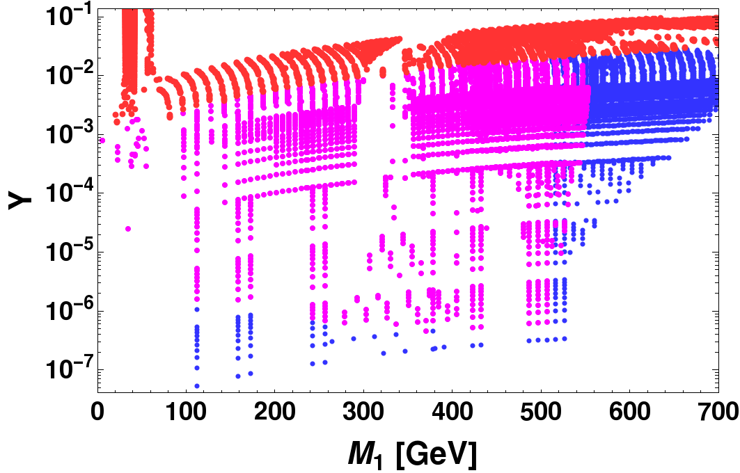
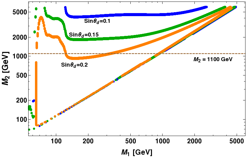
Figure 19: Left Panel: $Y$ vs $M_{1}$ scatter plot for correct relic density (Eq. 88). Here $\sin\theta_{d}$ ($10^{-6}$-0.2) and $\Delta M$ (1-1100 GeV) varies simultaneously. The top red points are disallowed by Lux 2016 direct search constraint. Both magenta and blue dots simultaneously satisfies relic density and Lux 2016 direct search constraints. The magenta dots additionally satisfies the condition $\Delta M<M_{W}$. Right Panel: $M_{1}$ versus $M_{2}$ (in GeV) for correct relic density. $\sin\theta_{d}=0.1,~{}0.2,~{}0.15$ (blue, green and orange respectively) has been chosen, while $\Delta M$ varies. The left panel is consistent with this plot upto $M_{2}$ = 1.1 TeV as marked by the horizontal dashed line in this plot.

In the left upper panel of Fig. 17, we plot the direct search cross-section against dark matter mass $M_{1}$ for a fixed choice of $\Delta M=100$ GeV. In this plot, we indicate regions allowed by direct search experimental limits. Since each point in the region allowed by direct search correspond to a specific relic density, once we incorporate both the relic density and direct search limit by LUX 2016, we find the allowed region is narrowed down as shown in the right upper panel of Fig. 17 (indicated by blue patch).

Similarly the left lower panel (left and right) of Fig. 17 shows the allowed (by both relic density and LUX 2016) region of parameter space where variation of $M_{2}$ is restricted up to 1.1 TeV with $\sin\theta_{d}\leq 0.2$. We find that an uper limit on $\sin\theta_{d}$ is prevailing from this plot. Combining relic density constraint and direct search limits, we find the allowed region indicated by blue dots in the right lower panel of Fig. 17. In order to obtain limits on $Y$ while $\Delta M$ and $\sin\theta_{d}$ are varied, we have provided a scatter plot of $Y$ versus $M_{1}$ in Fig. 19. In producing this plot, we have varied $M_{2}$ (up to 1.1 TeV), $10^{-7}<\sin\theta_{d}<0.2$. Here red dots correspond to those points which are disallowed by LUX 2016 even if these satisfy the relic density constraint. The blue patch indicates the region allowed by both the relic density and LUX 2016 data having $\Delta M>m_{W}$. For $\Delta M<m_{W}$, we use a lower limit on $\sin\theta_{d}$ obtained from Eq. (93). Hence the points in magenta satisfy the above $\sin\theta_{d}$ constraint and represent the allowed region by relic density and direct search limits. From this plot we can clearly see the upper limit of $Y$ is almost 0.03 while the lower limit of it can be very small, $\sim 10^{-7}$. Note that the $Y$ region limited by the choice of upper value of $M_{2}$ = 1.1 TeV is consistent with our earlier plot in Fig. 14 with fixed $\sin\theta_{d}$ values. For elaboration purpose, we provide the figure in the right panel of Fig. 19, which is the same plot as Fig. 14 except that it is now plotted in terms of $M_{2}$ vs. $M_{1}$. The narrow patch for a fixed $\sin\theta_{d}$ becomes wider as we varied $\sin\theta_{d}$ as well. The horizontal dashed line indicates our consideration of keeping the variation of $M_{2}$ within 1.1 TeV.

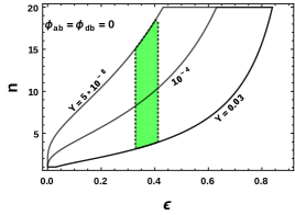
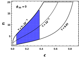
Figure 20: $n$ vs $\epsilon$ to generate different values of $Y=\epsilon^{n}$ for (a) $\phi_{db}=\phi_{ab}=0$ (left), (b) $\phi_{db}=0$ (middle) and (c) $\phi_{ab}=0$ (right).

We summarize here these constraints on $\epsilon$ and $Y=\epsilon^{n}$ to determine the unknown flavor charge $n$ of the dark matter in our scenario. It is shown in Fig. 20. Colored patch in each plot corresponds to the allowed range of $\epsilon$ obtained in section 3 for Cases A(D), B and C. In the left-most panel of Fig. 20, we have shown the allowed values of $n$ where the CP-violating phases are taken to be zero corresponding to Case A. As the direct search of DM restricts the $Y$ values to be $Y\lesssim 0.03$, we get $n\gtrsim 2$. Different contour lines with different $Y$ values are shown in the figure. A similar conclusion holds for the other case (Case D) with $\phi_{db}=\phi_{ab}=\beta$ . On the other hand, if $\phi_{ab}\neq\phi_{db}$ then a larger range of $n$ values are expected to be allowed. In particular, by setting $\phi_{db}=0$ and $\phi_{ab}\neq 0$ (as shown in middle panel of Fig. 20) we see that lower limit on $n$ starts from 1. On the other hand, if $\phi_{ab}=0$ and $\phi_{db}\neq 0$ (as shown in the right panel of Fig. 20) then $n$ can take values starting from 3. Thus we conclude that the non-zero values of phases introduce more uncertainty in specifying $n$. The future measurements of Dirac CP phase $\delta$ and a more stringent constraints from Direct search experiments would reduce this uncertainty in $n$.

6 Conclusions

In this paper we have explored a $U(1)$ flavor extension of the SM in order to establish a possible correlation between the SM sector (more specifically neutrino sector) and the DM one, in particular between the reactor lepton mixing angle $\sin\theta_{13}$ and the interaction of dark matter with SM Higgs. To start with, we have considered a tri-bimaximal mixing pattern ($i.e.$ with $\theta_{13}=0$) for the lepton mixing matrix originated from a typical flavor structure of the neutrino mass matrix guided by the non-Abelian flavor symmetry, where the charged lepton mass matrix is found to be diagonal. In its simplest version, we achieve the TBM structure of the neutrino mass matrix by assuming an $A_{4}\times Z_{3}$ symmetry where the effective dimension six operators involving $A_{4}$ flavons contributes to Majorana masses for light neutrinos. The symmetry forbids the usual dimension five operator. On the other hand, the dark sector consists of two vector-like fermions, one is a $SU(2)_{L}$ doublet and the other one is a SM gauge singlet. In addition we assume the existence of a $U(1)$ flavor symmetry under which the DM fields as well as two flavons, $\phi$ and $\eta$, are charged. It is interesting to note that with the vector-like fermions present in the dark sector, there exists a replica of SM Yukawa interaction in the dark sector which involves flavon $\phi$. The $U(1)$ symmetry of the model was broken at a high scale by the vev of that flavon field $\phi$ to a remnant $\mathcal{Z}_{2}$ under which the dark sector particles are odd. As a result the lightest odd particles becomes a viable candidate of dark matter. Moreover, a higher dimensional operator involving $\phi$ and $\eta$ constitutes a correction to the TBM pattern of the neutrino mass matrix which leads to a non-zero value of $\sin\theta_{13}$. The involvement of $\phi$ ensures that $B-L$ breaking vev is also involved in this correction term. As a result we are able to show that the non-zero value of $\sin\theta_{13}$ is proportional to the Higgs portal coupling, $Y=(\phi/\Lambda)^{n}\equiv\epsilon^{n}$, of the dark matter which gives rise to correct relic density measured by WMAP and PLANCK and consistent with direct DM search bound from LUX. Finally it is interesting to note that $Y$, on one hand is related to the mixing in the neutrino sector, while it also crucially controlled by the mixing involved in the dark sector. We also find that the current allowed values of $\sin\theta_{13}$ indicates the $U(1)$ charge of DM $\gtrsim 1$ which can be probed at the future direct DM search experiments such as Xenon-1T. The next to lightest stable particle (NLSP) is a charged fermion which can be searched at the LHC Arina:2012aj ; Arina2 . In the limit of small $\sin\theta_{d}$, the NLSP can give rise to a displaced vertex at LHC, a rather unique signature of the model discussed in ref. Bhattacharya:2015qpa . We argue that this is a minimal extension to SM to accommodate DM and non-zero $\sin\theta_{13}$ by using a flavor symmetric approach.

- (1) S. Fukuda et al. [Super-Kamiokande Collaboration], Phys. Lett. B 539, 179 (2002) [hep-ex/0205075].
- (2) Y. Ashie et al. [Super-Kamiokande Collaboration], Phys. Rev. D 71, 112005 (2005) [hep-ex/0501064].
- (3) P. Adamson et al. [MINOS Collaboration], Phys. Rev. Lett. 106, 181801 (2011) [arXiv:1103.0340 [hep-ex]].
- (4) T. Araki et al. [KamLAND Collaboration], Phys. Rev. Lett. 94, 081801 (2005) [hep-ex/0406035].
- (5) G. Hinshaw et al. [WMAP Collaboration], Astrophys. J. Suppl. 208, 19 (2013) [arXiv:1212.5226 [astro-ph.CO]].
- (6) P. A. R. Ade et al. Planck Collaboration, Astron. Astrophys. 571, A16 (2014), arXiv:1303.5076 [astro-ph.CO].
- (7) P. A. R. Ade et al. [Planck Collaboration], Astron. Astrophys. 594, A13 (2016) doi:10.1051/0004-6361/201525830 [arXiv:1502.01589 [astro-ph.CO]].
- (8) G. Bertone, D. Hooper and J. Silk, Phys. Rept. 405, 279 (2005), arXiv:hep-ph/0404175.
- (9) C. D. Froggatt and H. B. Nielsen, Nucl. Phys. B 147, 277 (1979).
- (10) E. Ma and G. Rajasekaran, Phys. Rev. D 64 (2001) 113012 [hep-ph/0106291].
- (11) G. Altarelli and F. Feruglio, Nucl. Phys. B 741, 215 (2006) [hep-ph/0512103].
- (12) F. Capozzi, G. L. Fogli, E. Lisi, A. Marrone, D. Montanino and A. Palazzo, Phys. Rev. D 89, no. 9, 093018 (2014) [arXiv:1312.2878 [hep-ph]].
- (13) M. C. Gonzalez-Garcia, M. Maltoni and T. Schwetz, JHEP 1411, 052 (2014) [arXiv:1409.5439 [hep-ph]].
- (14) D. V. Forero, M. Tortola and J. W. F. Valle, Phys. Rev. D 90, no. 9, 093006 (2014) [arXiv:1405.7540 [hep-ph]].
- (15) Y. Abe et al. [Double Chooz Collaboration], Phys. Rev. Lett. 108, 131801 (2012) [arXiv:1112.6353 [hep-ex]].
- (16) F. P. An et al. [Daya Bay Collaboration], Phys. Rev. Lett. 108, 171803 (2012) [arXiv:1203.1669 [hep-ex]].
- (17) J. K. Ahn et al. [RENO Collaboration], Phys. Rev. Lett. 108, 191802 (2012) [arXiv:1204.0626 [hep-ex]].
- (18) K. Abe et al. [T2K Collaboration], Phys. Rev. Lett. 112, 061802 (2014) [arXiv:1311.4750 [hep-ex]].
- (19) S. Bhattacharya, N. Sahoo and N. Sahu, Phys. Rev. D 93, no. 11, 115040 (2016) [arXiv:1510.02760 [hep-ph]].
- (20) S. Bhattacharya, B. Karmakar, N. Sahu and A. Sil, Phys. Rev. D 93, no. 11, 115041 (2016) [arXiv:1603.04776 [hep-ph]].
- (21) E. Aprile et al. [XENON Collaboration], [arXiv:1512.07501 [physics.ins-det]].
- (22) C. Arina, R. N. Mohapatra and N. Sahu, Phys. Lett. B 720 (2013) 130 [arXiv:1211.0435 [hep-ph]].
- (23) C. Arina, J. O. Gong and N. Sahu, Nucl. Phys. B 865, 430 (2012) [arXiv:1206.0009 [hep-ph]].
- (24) S. F. King and C. Luhn, JHEP 1109, 042 (2011) [arXiv:1107.5332 [hep-ph]].
- (25) M. Holthausen, M. Lindner and M. A. Schmidt, Phys. Rev. D 87, no. 3, 033006 (2013) [arXiv:1211.5143 [hep-ph]].
- (26) L. Dorame, S. Morisi, E. Peinado, J. W. F. Valle and A. D. Rojas, Phys. Rev. D 86, 056001 (2012) [arXiv:1203.0155 [hep-ph]].
- (27) P. F. Harrison, D. H. Perkins and W. G. Scott, Phys. Lett. B 458, 79 (1999) [hep-ph/9904297].
- (28) B. Karmakar and A. Sil, Phys. Rev. D 91, 013004 (2015) [arXiv:1407.5826 [hep-ph]].
- (29) G. C. Branco, R. Gonzalez Felipe, F. R. Joaquim and H. Serodio, Phys. Rev. D 86, 076008 (2012) [arXiv:1203.2646 [hep-ph]].
- (30) B. Karmakar and A. Sil, Phys. Rev. D 93, no. 1, 013006 (2016) [arXiv:1509.07090 [hep-ph]].
- (31) B. Karmakar and A. Sil, arXiv:1610.01909 [hep-ph].
- (32) Y. Shimizu, M. Tanimoto and A. Watanabe, Prog. Theor. Phys. 126, 81 (2011) [arXiv:1105.2929 [hep-ph]].
- (33) L. Calibbi, A. Crivellin and B. Zaldívar, Phys. Rev. D 92, no. 1, 016004 (2015) [arXiv:1501.07268 [hep-ph]].
- (34) M. Hirsch, S. Morisi, E. Peinado and J. W. F. Valle, Phys. Rev. D 82, 116003 (2010) [arXiv:1007.0871 [hep-ph]].
- (35) M. S. Boucenna, M. Hirsch, S. Morisi, E. Peinado, M. Taoso and J. W. F. Valle, JHEP 1105, 037 (2011) [arXiv:1101.2874 [hep-ph]]
- (36) R. de Adelhart Toorop, F. Bazzocchi and S. Morisi, Nucl. Phys. B 856, 670 (2012) [arXiv:1104.5676 [hep-ph]].
- (37) Y. Hamada, T. Kobayashi, A. Ogasahara, Y. Omura, F. Takayama and D. Yasuhara, JHEP 1410, 183 (2014) [arXiv:1405.3592 [hep-ph]].
- (38) W. C. Huang, JHEP 1411, 083 (2014) [arXiv:1405.5886 [hep-ph]].
- (39) M. Lattanzi, R. A. Lineros and M. Taoso, New J. Phys. 16, no. 12, 125012 (2014) [arXiv:1406.0004 [hep-ph]].
- (40) I. de Medeiros Varzielas, O. Fischer and V. Maurer, JHEP 1508, 080 (2015) [arXiv:1504.03955 [hep-ph]].
- (41) E. Ma, Phys. Lett. B 754, 114 (2016) [arXiv:1506.06658 [hep-ph]].
- (42) I. Medeiros Varzielas and O. Fischer, JHEP 1601, 160 (2016) [arXiv:1512.00869 [hep-ph]].
- (43) A. Mukherjee and M. K. Das, Nucl. Phys. B 913, 643 (2016) [arXiv:1512.02384 [hep-ph]].
- (44) J. M. Lamprea and E. Peinado, arXiv:1603.02190 [hep-ph].
- (45) G. Altarelli and F. Feruglio, Rev. Mod. Phys. 82, 2701 (2010) [arXiv:1002.0211 [hep-ph]].
- (46) K. Griest and D. Seckel, Phys. Rev. D 43, 3191 (1991); A. Chatterjee and N. Sahu, Phys. Rev. D 90, no. 9, 095021 (2014) [arXiv:1407.3030 [hep-ph]].
- (47) G. Cynolter and E. Lendvai, Eur. Phys. J. C 58, 463 (2008) [arXiv:0804.4080 [hep-ph]].
- (48) T. Cohen, J. Kearney, A. Pierce and D. Tucker-Smith, Phys. Rev. D 85, 075003 (2012) [arXiv:1109.2604 [hep-ph]].
- (49) C. Cheung and D. Sanford, JCAP 1402, 011 (2014) [arXiv:1311.5896 [hep-ph]].
- (50) G. Belanger, F. Boudjema, A. Pukhov and A. Semenov, Comput. Phys. Commun. 180, 747 (2009) [arXiv:0803.2360 [hep-ph]].
- (51) M. W. Goodman and E. Witten, Phys. Rev. D 31, 3059 (1985).
- (52) R. Essig, Phys. Rev. D 78, 015004 (2008) [arXiv:0710.1668 [hep-ph]].
- (53) R. Koch, Z. Phys. C 15, 161 (1982),
- (54) J. Gasser, H. Leutwyler and M. E. Sainio, Phys. Lett. B 253, 260 (1991).
- (55) M. M. Pavan, I. I. Strakovsky, R. L. Workman and R. A. Arndt, PiN Newslett. 16, 110 (2002) [hep-ph/0111066].
- (56) A. Bottino, F. Donato, N. Fornengo and S. Scopel, Phys. Rev. D 78, 083520 (2008) [arXiv:0806.4099 [hep-ph]].
- (57) D. S. Akerib et al., arXiv:1608.07648 [astro-ph.CO].
- (58) K. A. Olive et al. [Particle Data Group Collaboration], Chin. Phys. C 38, 090001 (2014).
- (59) A. S. Joshipura and J. W. F. Valle, Nucl. Phys. B 397, 105 (1993).
- (60) G. Aad et al. [ATLAS Collaboration], JHEP 1601, 172 (2016) doi:10.1007/JHEP01(2016)172 [arXiv:1508.07869 [hep-ex]].
- (61) V. Khachatryan et al. [CMS Collaboration], JHEP 1702, 135 (2017) doi:10.1007/JHEP02(2017)135 [arXiv:1610.09218 [hep-ex]].
- (62) C. P. Burgess, M. Pospelov and T. ter Veldhuis, Nucl. Phys. B 619, 709 (2001) doi:10.1016/S0550-3213(01)00513-2 [hep-ph/0011335].
- (63) M. Frigerio, T. Hambye and E. Masso, Phys. Rev. X 1, 021026 (2011) doi:10.1103/PhysRevX.1.021026 [arXiv:1107.4564 [hep-ph]].
- (64) L. J. Hall, K. Jedamzik, J. March-Russell and S. M. West, JHEP 1003, 080 (2010) doi:10.1007/JHEP03(2010)080 [arXiv:0911.1120 [hep-ph]].