Generalized Radon–Nikodym Spectral Approach. Application to Relaxation Dynamics Study.

Abstract

Radon–Nikodym approach to relaxation dynamics, where probability density is built first and then used to calculate observable dynamic characteristic is developed and applied to relaxation type signals study. In contrast with $L^{2}$ norm approaches, such as Fourier or least squares, this new approach does not use a norm, the problem is reduced to finding the spectrum of an operator (virtual Hamiltonian), which is built in a way that eigenvalues represent the dynamic characteristic of interest and eigenvectors represent probability density. The problems of interpolation (numerical estimation of Radon–Nikodym derivatives is developed) and obtaining the distribution of relaxation rates from sampled timeserie are considered. Application of the theory is demonstrated on a number of model and experimentally measured timeserie signals of degradation and relaxation processes. Software product, implementing the theory is developed.

I Introduction

For the problem of relaxation signals study the determination of dynamic characteristics from experimentally collected data is critically important in applications. Initial data, typically collected in a form of timeseries, is often analyzed applying such common techniques as regressional analysis, Fourier/Laplace analysis, wavelet analysis, Machine Learning, distribution extreme value analysis, among many others. In this paper we developed, implemented in software and demonstrated in applications a new calculus-like technique[1], Radon–Nikodym derivatives (and their generalization), to relaxation dynamics problems. This technique is extremely effective in relaxation signals study, where other approaches (such as Fourier/Laplace analysis) are poorly applicable. The synergy between Radon–Nikodym derivatives and numerical analysis (computer software implementation is provided) as well as approach effectiveness to relaxation processes study are the the most important features. Without apriori assumptions (such us the number or different relaxation rates) the distribution of key dynamics characteristics of sampled signal (such as relaxation times, time derivative, etc.) can be directly obtained from timeserie. The approach is reducible to matrix spectrum problem (without any $L^{2}$ norm involved), and the distribution of dynamics characteristics can be obtained from the distribution of eigenvalues in spectrum. To the best of our knowledge this is the only practical approach allowing to obtain the distribution of relaxation rates from sampled data without apriori assumptions. Other approaches are not applicable for these reasons:

• Fourier/Wavelet transform cannot be effectively applied to relaxation data study. If basis dimension is chosen high enough, then yes, all information is accumulated in components, but, in contrast with oscillatory type of signals, the distribution of relaxation rates cannot be obtained from the distribution of Fourier components.

• Laplace analysis is applicable only analytically, for sampled data discretization, rounding errors and sample finite size make Laplace approach inapplicable.

• ‘‘Fitting the curve’’ type of approaches can be effectively applied to the data such as in Figs. 2 and 4, but only with apriori knowledge about the number of different relaxation rates in sample (i.e. two in Fig. 2 and three in Fig. 4). Without this information, e.g. with multiple rates as in Fig. 7, any ‘‘fitting the curve’’ approach fails.

• Re–sampling techniques (such as take initial $(x_{l},f_{l})$ timeserie and re-sample it to obtain derivative timeserie $(x_{l},(f(x_{l})-f(x_{l}-\tau))/\tau)$ typically fail for inability to choose the parameter $\tau$. For real life data (such as presented in Fig. 7) a good $\tau$ value does not exist.

• Additional important feature of our approach, is that it does not deploy any $L^{2}$ norm (as Fourier or least squares do), it uses operator spectrum instead. The approach is norm–free. For this reason it is not sensitive to sample outliers thus can be effectively applied to non–Gaussian samples, e.g. even with infinite second moment of dynamic characteristics in study.

Java written computer implementation is provided. The code reads timeserie data input $(x_{l},f_{l})$, construct ‘‘virtual quantum system Hamiltonian’’, corresponding to dynamic characteristics of interest ($f$, $df/dx$ or $(df/dx)/f$), diagonalize this ‘‘Hamiltonian’’ and output its spectrum. The distribution of dynamic characteristics of interest is described by the distribution of obtained spectrum, similar to the situation in random matrix theory[2]. An application is demonstrated on a number of practical examples, including both model data and real life data of degradation and relaxation dynamics problems.

II Radon–Nikodym Interpolation Problem

Let us start with the simplest possible problem: interpolation problem. Consider some timeserie ($x$ is time) of $M$ observations total

$$x_{l} \to f_{l}$$ (1)

$$l = 1\dots M$$

$$x_{l} \leq x_{l+1}$$

Interpolation problem is to estimate at given $x$ the $f(x)$ and $df/dx$ using the data (1). First we need some basis $Q_{k}(x)$, in this paper we will be using polynomial bases. The results are invariant with respect to basis choice (e.g. $Q_{k}(x)=x^{k}$ give identical result), but numerical stability, especially in high dimension, depends strongly on basis choice[1], and the bases like Chebyshev or Legendre polynomials have to be used in numerical calculations (see appendix A for discussion). Given the basis $Q_{k}(x)$ and observation weight function $\omega(x)$ (in this paper $\omega(x)=1$), obtain the moments:

$$\Braket{Q_{k}} = \sum_{l=1}^{M}Q_{k}(x_{l})(x_{l}-x_{l-1})\omega(x_{l})$$ (2)

$$\Braket{fQ_{k}} = \sum_{l=1}^{M}Q_{k}(x_{l})(x_{l}-x_{l-1})f_{l}\omega(x_{l})$$ (3)

$$\Braket{df/dxQ_{k}} = \sum_{l=1}^{M}Q_{k}(x_{l})(f_{l}-f_{l-1})\omega(x_{l})$$ (4)

Given these moments Gramm matrix $G_{jk}=\Braket{Q_{j}Q_{k}}$ and the matrices $\Braket{fQ_{j}Q_{k}}$ and $\Braket{df/dxQ_{j}Q_{k}}$ can be readily obtained either directly from (2), (3) and (4) sums with $Q_{j}(x)Q_{k}(x)$ term, or, more computationally efficient, using basis multiplication operator (the $c_{l}^{jk}$ coefficients are available analytically for all practically interesting bases, see Appendix A of Ref. [3] and references therein) and first $2n-1$ moments $\Braket{Q_{l}}$, $\Braket{fQ_{l}}$ and $\Braket{df/dxQ_{l}}$; $l=[0\dots 2n-2]$.

$$Q_{j}(x)Q_{k}(x) = \sum_{l=0}^{j+k}c_{l}^{jk}Q_{l}(x)$$ (5)

Standard least squares interpolation $A_{LS}(y)$ is then:

$$A_{LS}(y) = \sum\limits_{i,j=0}^{n-1}Q_{i}(y)\left(G^{-1}\right)_{ij}\Braket{gQ_{j}}$$ (6)

here $G^{-1}$ is a matrix inverse to Gramm matrix $\Braket{Q_{j}Q_{k}}$, the $g$ is either $f$ of $df/dx$ depending on what need to be interpolated, and $n$ is the dimension chosen. Then the $A_{LS}(y)$ is $n-1$ order polynomial interpolating the function $g(y)$. The (6) is direct interpolation of observable $g$, obtained from minimization of $L^{2}$ norm (cost function[4]) $\Braket{\left(g(x)-\sum_{i=0}^{n-1}\alpha_{i}Q_{i}(x)\right)^{2}}\to\min$ on $\alpha_{i}$, what give $A_{LS}(y)=\sum_{i=0}^{n-1}\alpha_{i}Q_{i}(y)$ in the form (6)).

Radon–Nikodym interpolation $A_{RN}(y)$ is:

$$A_{RN}(y)=\frac{\sum\limits_{i,j,k,m=0}^{n-1}Q_{i}(y)\left(G^{-1}\right)_{ij}\Braket{gQ_{j}Q_{k}}\left(G^{-1}\right)_{km}Q_{m}(y)}{\sum\limits_{i,j=0}^{n-1}Q_{i}(y)\left(G^{-1}\right)_{ij}Q_{j}(y)}$$ (7)

The (7) is a ratio of two polynomials of $2n-2$ order each, an estimator of stable form[5]. In contrast with $A_{LS}(y)$, which is obtained as one–stage interpolation of observable $g$, the $A_{RN}(y)$ is obtained in two stages:

• Obtain localized at $x=y$ probability density $\rho_{y}(x)=\psi^{2}_{y}(x)$, where

  $$\psi_{y}(x) = \sum\limits_{i,j=0}^{n-1}Q_{i}(x)\left(G^{-1}\right)_{ij}Q_{j}(y)$$ (8)

  is localized at $x=y$. The (8) is actually identical to least squares answer (6) with the replacement of $\Braket{gQ_{j}}$ by $Q_{j}(y)$. Also note that $1/\psi_{x}(x)$ is equal to Christoffel function, which define Gauss quadratures weights[6] for the measure $d\mu=\omega(x)dx$.

• Average $g(x)$ with obtained probability density as

  $$A_{RN}(y)=\frac{\Braket{\rho_{y}(x)g(x)}}{\Braket{\rho_{y}(x)}}=\frac{\int\psi_{y}^{2}(x)g(x)\omega(x)dx}{\int\psi_{y}^{2}(x)\omega(x)dx}$$ (9)

  to obtain (7) as a ratio of two quadratic forms, the ratio of two polynomials of $2n-2$ order in case of polynomial basis.

The answer (7) is plain Nevai operator[7] (with its property of absolute convergence to $g(x)$ with $n$ increase) and can be viewed as numerical estimation of $\frac{d\mu}{d\nu}=\frac{gdx}{dx}$ considered as Radon–Nikodym derivative[8]. The (7) answer is typically the most convenient one among other available, because it requires only one measure $d\nu$ to be positive. Other answers[9, 3] require both measures $d\mu$ and $d\nu$ to be positive. This Radon–Nikodym interpolation (7) has several critically important advantages[3, 10, 1] compared to least squares interpolation (6): stability of interpolation, there is no divergence outside of interpolation interval, oscillations near interval edges are very much suppressed, even in multi–dimensional case[10]. These advantages come from the very fact, that probability density is interpolated first, then the result is obtained by averaging with this, always positive, interpolated probability.

Another issue should be stressed here. For $df/dx$ interpolation one should use the (4) moments for $g=df/dx$. If one, instead of direct interpolation of $g=df/dx$, interpolate $g=f$ (using (3) moments) and then differentiate interpolating expression (6) or (7) the result will be incorrect[10].

II-A Demonstration of Radon–Nikodym Interpolation in 1D and 2D cases

Before we go further let us demonstrate the result of Radon–Nikodym interpolation on standard data set[10] in 1D and 2D cases.

Consider (often used for algorithms testing) Runge function

$$f(x)=\frac{1}{1+25x^{2}}$$ (10)

with the measures

$$\Braket{fQ_{k}} = \int_{-1}^{1}f(x)Q_{k}(x)dx$$ (11)

$$\Braket{df/dxQ_{k}} = \int_{-1}^{1}\frac{df(x)}{dx}Q_{k}(x)dx$$ (12)

Then apply (6) and (7) interpolating formulas. The results are presented in Fig.1.

Figure 1: Top:Least squares $A_{LS}$ and Radon–Nikodym $A_{RN}$ approximations for Runge function(left) and Runge function derivative (right) for $n=7$. Bottom: Original Lenna image, least squares and Radon-Nikodym for $n_{x}=n_{y}=50$.

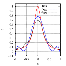
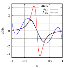
In Fig. 1 least squares and Radon–Nikodym interpolations are presented for $n=7$ and the measures (11) and (12). One can see that near edges oscillations are much less severe, when Radon–Nikodym approximation (polynomials ratio) is used for interpolation. This is because of the very fact that Radon–Nikodym approximation has probability (not the observable value) interpolated, and the result is obtained by averaging with this, always positive, probability density.

Consider 2D case of image grayscale intensity interpolation for Lenna 512x512 image[11] (presented in Fig. 1). As a measure use the sum over image pixels $(t_{x},t_{y})$ and consider basis index as double index $\bm{k}=(k_{x},k_{y})$:

$$\Braket{fQ_{\bm{k}}}=\sum_{t_{x}=0}^{d_{x}-1}\sum_{t_{y}=0}^{d_{y}-1}f(t_{x},t_{y})Q_{k_{x}}(t_{x})Q_{k_{y}}(t_{y})$$ (13)

With a proper $Q_{\bm{k}}$ basis selection[10] numerically stable results can be obtained for up to $100\times 100$ elements in basis, i.e. for $10,000$ basis functions. The least squares interpolation, same as in 1D case, present typical for least squares intensity oscillations near image edges, while Radon–Nikodym has these oscillations very much suppressed. Another important feature of Radon–Nikodym is that it preserves the sign of interpolated function, i.e. the grayscale intensity $f$ never become negative, what may happen easily for least squares.

The difference between Radon–Nikodym and least squares are of qualitative type and can be summarized as following:

• For Radon–Nikodym (7) interpolated value at $y$ is sample data averaged with positive weight $d\mu_{\psi}=\psi_{y}^{2}(x)\omega(x)dx$ localized at $y$ (8), i.e. it is some weighted combination of sample observations. Least squares (6) interpolation does not correspond to a weighted combination of sample observations. This lead to interval edge oscillations being very much suppressed for Radon–Nikodym.

• Radon–Nikodym is a ratio of two quadratics forms built on basis functions. Least squares is a linear combination of basis functions. This lead to interpolation function sign preservation and no divergence at $y\to\infty$ for Radon–Nikodym.

• Because Radon–Nikodym does not deploy any $L^{2}$ norm it is much less sensitive to data outliers. For least squares even a single data outlier can completely break the result.

• Radon–Nikodym requires more computational resources: $n\times n$ matrix $\Braket{gQ_{j}Q_{k}}$ (obtained from first $2n-1$ input moments) vs. a vector of first $n$ input moments $\Braket{gQ_{j}}$ for least squares.

• Most important, Radon–Nikodym can be generalized as an approach where learned knowledge is stored in matrix spectrum and then extracted using projection operators. This to be considered next.

III Generalized Radon–Nikodym. Quantum Mechanical Spectral Description of Classical Experiment

Considered in section II interpolation problem is the first application of Radon–Nikodym approach. The key element of the approach is that it based on matrices $\Braket{Q_{j}Q_{k}}$ and $\Braket{gQ_{j}Q_{k}}$, not vectors $\Braket{gQ_{j}}$, as in least squares (6). The answers (6) and (7) are written in arbitrary polynomial basis $Q_{i}(x)$. However the matrix approach allow us to introduce special, ‘‘natural basis (17)’’ $\psi^{[i]}(x)$, that diagonalize the matrices $\Braket{Q_{j}Q_{k}}$ and $\Braket{gQ_{j}Q_{k}}$ simultaneously. Consider Hamiltonian of a quantum system, the eigenfunctions of which (17), are the solutions of generalized eigenvalues problem (16), and diagonalize[12] these two matrices simultaneously $\Braket{\psi^{[i]}\psi^{[j]}}=\delta_{ij}$ and $\Braket{g\,\psi^{[i]}\psi^{[j]}}=\lambda^{[i]}\delta_{ij}$

$$M^{L}_{jk}=\Braket{g\,Q_{j}Q_{k}}$$ (14)

$$M^{R}_{jk}=\Braket{Q_{j}Q_{k}}$$ (15)

$$\sum\limits_{k=0}^{n-1}M^{L}_{jk}\alpha^{[i]}_{k}=\lambda^{[i]}\sum\limits_{k=0}^{n-1}M^{R}_{jk}\alpha^{[i]}_{k}$$ (16)

$$\psi^{[i]}(x)=\sum\limits_{k=0}^{n-1}\alpha^{[i]}_{k}Q_{k}(x)$$ (17)

$$A_{RN}(y)=\frac{\sum\limits_{i=0}^{n-1}\lambda^{[i]}\left(\psi^{[i]}(y)\right)^{2}}{\sum\limits_{i=0}^{n-1}\left(\psi^{[i]}(y)\right)^{2}}$$ (18)

$$A_{LS}(y)=\sum\limits_{i=0}^{n-1}\psi^{[i]}(y)\Braket{g\,\psi^{[i]}}$$

$$=\sum\limits_{i=0}^{n-1}\lambda^{[i]}\psi^{[i]}(y)\Braket{\psi^{[i]}}$$ (19)

Probability states $\psi^{[i]}(x)$ from (17) are normalized in a usual way: $\sum_{j,k=0}^{n-1}\alpha^{[s]}_{j}M^{R}_{jk}\alpha^{[t]}_{k}=\delta_{st}$ and $\sum_{j,k=0}^{n-1}\alpha^{[s]}_{j}M^{L}_{jk}\alpha^{[t]}_{k}=\lambda^{[t]}\delta_{st}$. The (18) and (19) are identical to (7) and (6), but written in the basis of eigenfunctions $\psi^{[i]}(x)$ of (16) Hamiltonian. This interpretation of Radon–Nikodym interpolation (7) as obtaining two matrices from experimental observations, introduction of (defined by two these matrices) Hamiltonian of a quantum system, diagonalization (16) and obtaining (18) as an average with weights equal to the square of projection (because $\psi^{[i]}(y)=\Braket{\psi_{y}(x)\psi^{[i]}(x)}$ ; also note that Christoffel function is $1/\sum\limits_{i=0}^{n-1}\left(\psi^{[i]}(y)\right)^{2}$) of a state with specific $y$ (8) to eigenfunction (17) is very fruitful. The knowledge, obtained from the data, is now accumulated in matrix spectrum, and then can be extracted by projection operators. This give a number of important advantages[1] with respect to standard approaches, such as representation of learned knowledge in regression coefficients.

However, the most important generalization of the approach is to go from localized $\psi_{y}(x)$ states (8) to arbitrary $\psi(x)$, e.g. the (17) eigenvectors. Then, for example, minimal, maximal and average value of $g$ can be easily estimated as $\min\lambda^{[i]}$, $\max\lambda^{[i]}$ and $\sum_{i=0}^{n-1}\lambda^{[i]}/n$. This is drastically different from, say, regressional type of approach where only function interpolation can be obtained from sample moments. Obtained $\lambda^{[i]}$ spectrum can be interpreted as the distribution of $g$ from sample, what give a number of advantages in relaxation processes study. For example[13], consider $n=2$, then, like a difference between median and average, generalized skewness estimator of a $g(x)$ process can be introduced:

$$\widetilde{\Gamma} = \frac{2\overline{g}-\lambda^{[\min]}-\lambda^{[\max]}}{\lambda^{[\min]}-\lambda^{[\max]}}$$ (20)

$$\overline{g} = \frac{\Braket{gQ_{0}}}{\Braket{Q_{0}}}$$ (21)

Regular skewness estimator $\Braket{\left(g-\overline{g}\right)^{3}}$ requires 4 moments to calculate $\Braket{1}$, $\Braket{g}$ $\Braket{g^{2}}$, $\Braket{g^{3}}$ and is not applicable to strongly non–Gaussian processes, e.g. those with infinite $\Braket{g^{2}}$ or $\Braket{g^{3}}$. The $\widetilde{\Gamma}$ skewness estimator requires 6 moments to calculate: $\Braket{Q_{0}}$, $\Braket{Q_{1}}$, $\Braket{Q_{2}}$, $\Braket{gQ_{0}}$, $\Braket{gQ_{1}}$, $\Braket{gQ_{2}}$, (all of them are finite, even when $\Braket{g^{2}}$ is infinite). The $2\times 2$ matrices $\Braket{gQ_{j}Q_{k}}$ and $\Braket{Q_{j}Q_{k}}$ can be readily obtained from these moments, eigenvalues problem (16) solved by solving quadratic equation $0=\det\|\Braket{gQ_{j}Q_{k}}-\lambda\Braket{Q_{j}Q_{k}}\|$; $\min g=\lambda^{[\min]}$, $\max g=\lambda^{[\max]}$ obtained, and $\widetilde{\Gamma}$ from (20) calculated. When $Q_{k}(x)=Q_{k}(g)$ the $\widetilde{\Gamma}$ is proportional to regular skewness estimator. In this case only 4 out of 6 moments required for $\widetilde{\Gamma}$ calculation are independent. Another important result of the approach is a ‘‘replacement to standard deviation’’ as $\lambda^{[\max]}-\lambda^{[\min]}$, that is finite even for the processes with infinite $\Braket{g^{2}}$. This make the approach extremeny attractive to the study of signals with spikes [14].

III-A Quantum Mechanical Approach to Global Optimization Problem

The Radon–Nikodym approach also give a new look to optimization problem[3]. Instead of regualar optimization problem

$$g(\bm{x}) \to \min$$ (22)

Consider optimization problem in ‘‘quantum mechanics style’’ (note argument and basis function index can be considered multi-dimensional, e.g. $Q_{{\bm{k}}}(\bm{x})=Q_{k_{x}}(x)Q_{k_{y}}(y)Q_{k_{z}}(z)\dots$):

$$\psi(\bm{x})=\sum_{\bm{k}}\alpha_{\bm{k}}Q_{\bm{k}}(\bm{x})$$ (23)

$$d\mu_{\psi}=\psi^{2}(\bm{x})\omega(\bm{x})d\bm{x}$$ (24)

$$\frac{\Braket{g(\bm{x})\psi^{2}(\bm{x})}}{\Braket{\psi^{2}(\bm{x})}}\to\min$$ (25)

$$\frac{\sum_{{\bm{jk}}}\alpha_{\bm{j}}\Braket{g(\bm{x})Q_{\bm{j}}(\bm{x})Q_{\bm{k}}(\bm{x})}\alpha_{\bm{k}}}{\sum_{{\bm{jk}}}\alpha_{\bm{j}}\Braket{Q_{\bm{j}}(\bm{x})Q_{\bm{k}}(\bm{x})}\alpha_{\bm{k}}}\to\min$$ (26)

Instead of solving (22): find $\bm{x}$ providing minimal $g$, solve (25) instead: find probability state (a wavefunction $\psi(\bm{x})$) (23), providing minimal expected $g$ (25). After expansion to (26) obtain generalized eigenvalues problem (16) with $M^{L}_{\bm{jk}}=\Braket{g(\bm{x})Q_{\bm{j}}(\bm{x})Q_{\bm{k}}(\bm{x})}$ and $M^{R}_{\bm{jk}}=\Braket{Q_{\bm{j}}(\bm{x})Q_{\bm{k}}(\bm{x})}$, that can be efficiently solved numerically[12]. The result is $\psi^{[\min]}(\bm{x})$, corresponding to minimal eigenvalue $\lambda^{[\min]}$, providing probability distribution (24), not some specific $\bm{x}$ value as when solving (22) problem directly. The answer in a form of probability distribution is typically the most convenient in applications (because it allows to decouple observable $g$ (or $\bm{x}$) and probability) and used in other techniques, such as Bayesian Learning. If, for any reason, the $\bm{x}$, corresponding to found probability distribution is required, it can be estimated as

$$\bm{x}^{[\min]}_{est} = \frac{\Braket{\left(\psi^{[\min]}(\bm{x})\right)^{2}\bm{x}}}{\Braket{\left(\psi^{[\min]}(\bm{x})\right)^{2}}}$$ (27)

and global minimum of $g$ can be estimated as $\lambda^{[\min]}$. The $\bm{x}^{[\min]}_{est}$, besides being interpreted as optimization answer, can also be used by other optimization algorithms as starting value. Another interesting research topic is the roots of $\psi^{[\min]}(\bm{x})$. The value of $g$ is large near $\psi^{[\min]}(\bm{x})$ roots, which typically correspond to the ‘‘spikes’’ in $g$. This is especially simple in 1D case with polynomial basis[3]: for a given $n$ the $\psi^{[\min]}(x)$ ($n-1$ order polynomial) has exactly $n-1$ simple real distinct roots (but not necessary on the support of the measure $d\mu=\omega(x)dx$).

Other than $\psi^{[\min]}(\bm{x})$ eigenvectors of (16) are also of interest in applications. First order variation (30) of Rayleigh quotient is equal to zero, because of (16). Second order variation of Rayleigh quotient has a simple form (31), which is positive for arbitray $\delta\psi$ when $i=\min$ (global minimum $\lambda^{[\min]}$).

$$\psi = \psi^{[i]}(\bm{x})+\delta\psi$$ (28)

$$\frac{\Braket{g(\bm{x})\psi^{2}}}{\Braket{\psi^{2}}} = \lambda^{[i]}$$ (29)

$$+ 2\left[\Braket{g(\bm{x})\psi^{[i]}\delta\psi}-\lambda^{[i]}\Braket{\psi^{[i]}\delta\psi}\right]$$ (30)

$$+ \left[\Braket{g(\bm{x})\left(\delta\psi\right)^{2}}-\lambda^{[i]}\Braket{\left(\delta\psi\right)^{2}}\right]+\dots$$ (31)

All found $\psi^{[i]}(\bm{x})$ states (17) correspond to $\min$, $\max$ or saddle point of $g$ (first order variation (30) is zero) with respect to wavefunction variation (28). Thus this technique can be considered as a type of differential calculus (generalized Radon–Nikodym). This calculus variate probability state (wavefunction (28)), not $g(\bm{x}+\delta\bm{x})$ argument, as regular calculus does. This transition from $\bm{x}+\delta\bm{x}$ variation to wavefunction variation (28) allows to transform original optimization problem (22) in $\bm{x}$ space to Rayleigh quotient optimization (26) in $\psi(\bm{x})$ space and then to generalized eigenvalues problem (16), that can be efficiently solved numerically[12].

The approach of this paper works with (24) probability distribution. Bayesian Learning[4] works with $\rho(\bm{x}|\theta)$ parametric distribution. Despite both approaches work with probability distributions in $\bm{x}$ space, there are important conceptual differences between (25) approach and Bayesian Learning:

• Probability densities are represented only in (24) form. Original argument $\bm{x}$ enter to optimization problem (25) only via $\psi(\bm{x})$ components (23).

• There is no any norm or standard deviation $\sigma^{2}$ involved, what make our approach applicable to strongly non–Gaussian case.

• Unique ‘‘natural basis’’, the eigenvectors of (16) problem, can be considered as cluster centers. Predicted value can now be obtained as a superposition of projections[1] of these cluster centers to the state of interest, such as in Eq. (18) for interpolation problem.

• The $\bm{x}^{[\min]}_{est}$ answer (27) obtained using (24) distribution with $\psi^{[\min]}$ solution of (16), is some kind similar to $\rho(\bm{x}|\theta)$ parametric distribution used in Bayesian Learning[4], but is obtained from very different considerations.

• The (16) give global optimization solution $\psi^{[\min]}$ and the minimum is $\lambda^{[\min]}$.

Developed software (see Appendix A for description), besides the main goal of this study, obtaining relaxation rates distribution, can be also used for 1D optimization using the technique described. Output *_spectrum.dat files contain three columns: (index $i$, $\lambda^{[i]}$, $x^{[i]}_{est}$), calculated for all eigenstates $i=[0\dots n-1]$ of (16). The minimal eigenvalue ($i=0$) corresponds to the value of global minimum and corresponding $x^{[i]}_{est}$ is the (27) estimation.

There is an important extension of original problem from using input data in a form of timeserie (1), with $\bm{x}$ and $f$ being experimentally measured input variables, to the theory of distribution regression problem[15], where a bag of $\bm{x}$ observations, not a single $\bm{x}$ realization, is mapped to a single $f$:

$$(\bm{x}_{1},\bm{x}_{2},\dots,\bm{x}_{j},\dots,\bm{x}_{N})_{l} \to f_{l}$$ (32)

$$l = 1\dots M$$

The (32) can be considered as a distribution of $\bm{x}$ (a bag with $N$ realizations of $\bm{x}$ used as input) is mapped to a single $f$ value. The theory of above can be transformed[16, 17] to use a distributions of $\bm{x}$ as input. In [17] a generalization of formulas (7), (18) and (16) is obtained for this case. For distribution regression problem the (24) have a meaning of ‘‘the distribution of distribution’’ and can be effectively used in applications, such as to study the data with noise, the examples of Ref. [18] (drug activity prediction, content–based image classification, text categorization), and studied in Ref. [19] the concept of ‘‘volatility of volatility’’ that directly correspond to the distribution of distribution solution[17] of distribution regression problem. Similary, in case of global optimization in distribution regression problem, the solution of (25) give the distribution of $\bm{x}$–distribution, (24), providing minimal $g$.

IV Demonstration Of Radon–Nikodym Spectral Approach

The main idea of Radon–Nikodym Spectral Approach is to construct, from experimental observations, a ‘‘Quantum Mechanics Hamiltonian’’, the spectrum of which correspond to the dynamic characteristic of interest, then to study this Hamiltonian spectrum considering obtained eigenvalues distribution as a ‘‘density of states’’. Fourier analysis is different, it works with interpolation of an observable value (using $L^{2}$ norm) and harmonics are initially selected, not obtained from the data. Laplace analysis, in addition to the problems of Fourier analysis, has the problems of sample insufficient size and discretization noise, thus is not applicable to sampled data.

Radon–Nikodym Spectral Approach, same as quantum mechanics, constructs probability states, then observable variable characteristics are calculated using obtained probability densities. There is no any $L^{2}$ norm involved, what allows to study even strongly non–Gaussian distributions[1]. The main idea is to obtain from experimental data, such as (3) and (4), two matrices (not vectors like Fourier components or least squares coefficients). Then solve generalized eigenvalues problem (16) with these two matrices (diagonalize them simultaneously). Obtained eigenvalues spectrum provide the distribution of an observable. In random matrix theory[2] the goal is similar: to obtain matrix eigenvalues density, but the matrix in study is typically obtained from some initially selected model[20]. In this paper the $M^{L}_{jk}$ and $M^{R}_{jk}$ matrices, determining virtual Hamiltonian, are obtained directly from sampled signal data. Similary to random matrix theory eigenvalues density determine the distribution of the characteristic in study. Few examples of $M^{L}_{jk}$ and $M^{R}_{jk}$ choice (for practical implementation only one matrix $M^{L}_{jk}$ or $M^{R}_{jk}$ need to be positively defined).

• If $\Braket{Q_{j}df/dxQ_{k}}$ is used as $M^{L}_{jk}$ and $\Braket{Q_{j}Q_{k}}$ is used as $M^{R}_{jk}$ in (16) then the distribution of obtained $\lambda^{[i]}$; $i=[0..n-1]$ is the distribution of $df/dx$, observed in the data.

• If $\Braket{Q_{j}df/dxQ_{k}}$ is used as $M^{L}_{jk}$ and $\Braket{Q_{j}fQ_{k}}$ is used as $M^{R}_{jk}$ in (16) then the distribution of obtained $\lambda^{[i]}$; $i=[0..n-1]$ is the distribution of relaxation rates $\frac{df}{fdx}$ observed in the data.

• If $\Braket{Q_{j}\frac{d\ln(f)}{dx}Q_{k}}$ is used as $M^{L}_{jk}$ and $\Braket{Q_{j}Q_{k}}$ is used as $M^{R}_{jk}$ in (16) then the distribution of obtained $\lambda^{[i]}$; $i=[0..n-1]$ is the distribution of relaxation rates $\frac{df}{fdx}$ observed in the data.

• If $\Braket{Q_{j}xQ_{k}}$ is used as $M^{L}_{jk}$ and $\Braket{Q_{j}Q_{k}}$ is used as $M^{R}_{jk}$ in (16), then obtained eigenvalues $\lambda^{[i]}$; $i=[0..n-1]$ are the nodes and $1/\left(\psi^{[i]}(\lambda^{[i]})\right)^{2}$ are the weights of $n$–point Gauss quadrature built on $d\mu=\omega(x)dx$ measure[3] (also note that $\psi^{[i]}(x)$ from (17) are proportional to Lagrange interpolating polynomials: $\psi^{[i]}(\lambda^{[j]})=0$ for $i\neq j$). Because of this fact the software from appendix A can be used to build Gauss quadratures from sampled data.

Below we are going to demonstrate this spectral approach on several examples for both model and real life data. In practice relaxation data is most often obtained from the processes of degradation, relaxation, market dynamics, etc. We chose the following data for demonstration:

• Li-Ion degradation, subsection IV-A. This data is relatively easy to obtain experimentally, and, using accelerated cycling, degradation signals can be recorded in a period of few months. This make the system a good testbed degradation example, compared to other systems where degradation processes take decades.

• Supercapacitor discharge, subsection IV-B. Relaxation data in this system can be obtained in minutes, and, very important, the process is repeatable. In contrast with degradation process charge/discharge cycle can be repeated many times.

• Stock price changes, subsection IV-D. It is well known[21] that financial markets do not have any short–term time–scale and the distribution of market scales is actively studied[19]. This make interesting to apply our theory to market data, because we can obtain the distribution of price change rates directly from timeserie sample.

IV-A Li-Ion Degradation

Figure 2: Two stage degradation Li-Ion model with the slope on first and second stages $-0.01$ and $-0.1$ respectively. The stages length is 10:10 (equal time) for top chart and 15:5 for bottom chart. Corresponding distributions of $\lambda$ are calculated with $n=50$.

Figure 3: Degradation of LG Chem[22] Li-Ion battery. Left: dependence of battery capacity $f$ on cycle number $x$, and interpolation of degradation rate $df/dx$ using least squares (6) and Radon–Nikodym (7) interpolation for $df/dx$. Corresponding distributions of $\lambda$ are calculated with $n=50$.

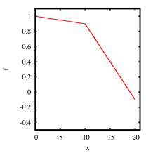
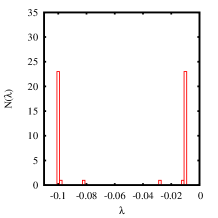
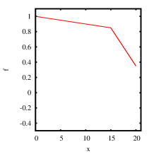
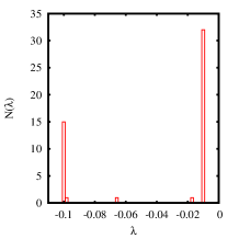
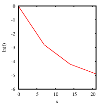
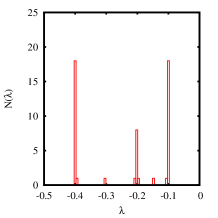
Consider typical for degradation dynamics a simple two–stage Li-Ion degradation model[23, 24], when battery capacity $C$ linearly decay with cycle number $N$, but the slope (degradation rate) changes at some point, see Fig. 2. To build a ‘‘Hamiltonian’’ the spectrum of which give degradation rate take $f=C$, $x=N$, $g=df/dx$, two matrices need to be calculated from experimental observations: $\Braket{Q_{j}df/dxQ_{k}}$ (4) to use it as $M^{L}_{jk}$ and $\Braket{Q_{j}Q_{k}}$ (2) as $M^{R}_{jk}$ in (16). Then $\lambda$ has exactly the meaning of degradation rate $df/dx$, and the distribution of it carry the information about available degradation rates in experimental observations. In Fig. 2 the distributions of $\lambda$, assuming all the eigenvalues have equal weights, are presented. These are two mode distributions with peaks at exact degradation rate of first and second stages: $\lambda=-0.01$ and $\lambda=-0.1$. Peak height growths with the increase of observations number at degradation rate value, but the dependence is more complicated than simple ratio of observations number. The relation was later found in Ref. [25] where the concept of Lebesgue integral quadrature was introduced. Each eignevalue $\lambda^{[i]}$ is considered as value–node $g_{i}$ of Lebesgue quadrature and corresponding weight $w_{i}$ are:

$$\Braket{g} = \sum\limits_{i=0}^{n-1}g_{i}\Braket{\psi^{[i]}}^{2}$$ (33)

$$g_{i} = \lambda^{[i]}$$ (34)

$$w_{i} = \Braket{\psi^{[i]}}^{2}$$ (35)

If instead of equal weights for $\lambda^{[i]}$ as in Fig. 2, one take Lebesgue quadrature wights (35) then, because we have chosen $d\mu=dN$ measure, distribution peaks height correspond exactly to stage length[25]. Lebesgue quadrature (33 can be considered as Lebesgue integral interpolating formula, by $n$–point discrete measure, the value–nodes $g_{i}$ select optimal positions of function values, they are $\|g\|$ operator eigenvalues (16), the weight $w_{i}$ is the measure of all $g\approx g_{i}$ sets. Note, that weights (35) give $\Braket{1}=\sum_{i=0}^{n-1}w_{i}$, same as for Gaussian quadrature weights.

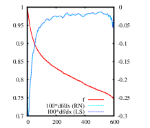
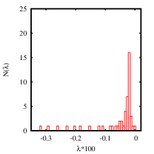
A more interesting data sample is real world Li-Ion degradation data. From [22] datasheet, battery capacity ($f$) as a function of cycle number ($x$) is obtained. Same as in the example above we build $\Braket{Q_{j}df/dxQ_{k}}$ and $\Braket{Q_{j}Q_{k}}$ matrices, from measured data, then use these matrices in (16) to obtain eigenvalues distribution. Eigenvalues disribution with Lebesgue weights (35) give spectrum distribution of ‘‘what was already observed’’ in degradation rates. The distribution with equal weight for each eigenvalue, Fig. 3, may serve as an idicator of ‘‘what can happen’’ to degradation rates. Strong difference in these distributions possibly indicate future drastic changes in degradation rate.

Least squares (6) and Radon–Nikodym (7) $df/dx$ interpolations are also calculated, they are presented in Fig. 3. The $df/dx$ data is smooth and both least squares and Radon–Nikodym give very similar result in interpolation of this specific example, not as with Lenna image in previous section.

IV-B Supercapacitor Discharge With Relaxation Time Change

Figure 4: Three stage modeled supercapacitor discharge. Stages exponents are $-0.4$, $-0.2$ and $-0.1$ with (36) and (37) matrix selection. The stages length is 7:7:7 (equal time) for top chart and 3.5:7.0:10.5 for bottom chart. Corresponding distributions of $\lambda$ are calculated with $n=50$.

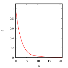
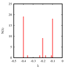
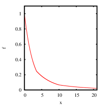
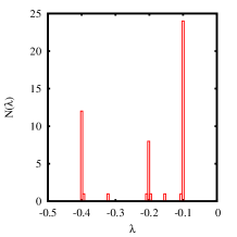
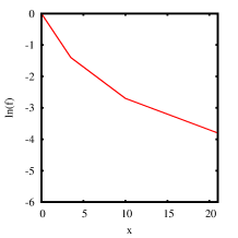
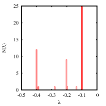
Consider a typical for relaxation dynamics multi–stage supercapacitor discharge, modeled with three consequential relaxation times as in Fig. 4. There are two alternative of discharge rate calculation. First, corresponding to $f^{\prime}/f$, approach

$$M^{L}_{jk} = \Braket{Q_{j}\frac{df}{dx}Q_{k}}$$ (36)

$$M^{R}_{jk} = \Braket{Q_{j}fQ_{k}}$$ (37)

and second, corresponding to $\ln(f)^{\prime}$, approach

$$M^{L}_{jk} = \Braket{Q_{j}\frac{d\ln(f)}{dx}Q_{k}}$$ (38)

$$M^{R}_{jk} = \Braket{Q_{j}Q_{k}}$$ (39)

Both selections give $\lambda$ as a discharge rate. The $\lambda$ has exactly the meaning of exponent ($\frac{df}{fdt}$) and the distribution of it carry the information about available exponents in experimental observations.

Consider first choice of ‘‘Hamiltonian’’. The matrices (36) and (37) are calculated from experimental observations as (4) and (3) to use them in (16); In Fig. 4 the distributions of $\lambda$ are presented at right. These are three mode distributions with peaks at exact exponents on first, second and third stages: $\lambda=-0.4$, $\lambda=-0.2$ and $\lambda=-0.1$. Peak height growths with observations number at the discharge rate, but, again, the dependence is more complicated than simple ratio of observations number, it is more similar to Christoffel function behavior[1].

In Fig. 5 the results corresponding to second matrix choice (38) and (39) are presented, same approach as in section IV-A above. The results in Figs. 4 and 5 are similar, but numerical stability of the results can be different in general case.

Figure 5: Three stage modeled supercapacitor discharge, same as in Fig. 5, but with (38) and (39) matrix selection.

We also want to note that instead of the basis $Q_{j}(x)$ a basis $Q_{j}(f(x))$ can be used. Similar technique was used in[26] for market dynamics study. The formulas are very similar to (3) and (4), e.g. we now have $\Braket{df/dxQ_{k}(f(x))}=\sum_{l=1}^{M}Q_{k}(f(x_{l}))(f_{l}-f_{l-1})\omega(x_{l})$ instead of (4). The $Q_{j}(x)$ and $Q_{j}(f(x))$ bases typically give very similar results for $n>10$, but numerical stability is often better for $Q_{j}(x)$ basis.

IV-C Supercapacitor With Track-Etched Membrane

Figure 6: Charging process of a supercapacitor with track-etched membrane. Potential $U$ as a function of time (top left). $dU/dt$ (bottom) calculated as (7) with $n=50$, $g=dU/dt$, $x=t$ and (4) moments. The distribution of $\lambda$ is calculated with $n=50$ (top right).

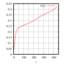
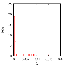
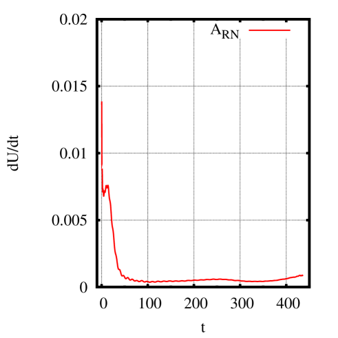
In Fig. 6 charging process data $U(t)$ with $I=2.5\cdot 10^{-5}$A for supercapacitor with superionic solid state electrolyte $RbAg_{4}I_{5}$ and track-etched membrane is presented. (Because electrolyte stability window of $RbAg_{4}I_{5}$ is $0.55-0.60$V, maximal charging potential is limited to $0.43$V. Charging time $436$sec.) This system can undergo multiple charge–discharge cycles and the measurement process can be completed under ten minutes. For these reasons this system is extemely convenient for relaxation type of signals study. Typical for supercapacitors two–stage $U(t)$ is seen on the chart. $dU/dt$ interpolation (using localized $\psi(x)$ from (8)) is calculated according to (7) with (4) moments. The most interesting is $dU/dt$ distribution chart, where the two intervals of different $\lambda$ are clearly seen.

IV-D Stock Price Changes

Figure 7: The logarithm of AAPL stock price on September, 20, 2012. $\lambda$ distribution of $d\ln P/dt$, calculated with $n=100$.

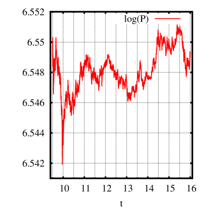
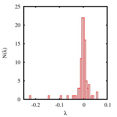
As we noted above the technique can be applies to arbitrary $f$ and $x$. Consider AAPL stock price on September, 20, 2012, same day we used in [3, 26] and obtain the distribution of $d(\ln P))/dx$, (here $x$ is time in hours). The result is presented in Fig. 7 for $n=100$. A very important feature of this approach is that it can be successfully applied to non–Gaussian distributions. The distribution of returns in Fig. 7 is clearly non–Gaussian, but, in contrast with all the $L^{2}$ approaches, matrix spectrum density analysis allows to estimate probability distribution even in a strongly non–Gaussian case[1]. To reproduce the result presented in Fig. 7 numerically see appendix A-B below.

V Radon–Nikodym Approach Applicability

There are several important issues, affecting results quality.

• Numerical instability. The problem arise typically for $n>4$ in monomials basis when calculating the moments (3) and (4), and then calculating $\Braket{Q_{j}gQ_{k}}$ from $\Braket{gQ_{k}}$ moments, what requires stable multiplication (5) of basis functions. With a proper basis choice (like Chebyshev or Legendre) the calculation are stable[27, 28, 3, 10] for $n$ up to 100-150 for 64bit double precision computer arithmetic. Stable calculations at even higher $n$ can be achieved with a transition to high–precision arithmetic.

• Data quality. While numerical instability in (3) and (4) can be overcome, missed data in the sample strongly affect the results.

• In situations, when high order derivatives are of interest, a special care should be taken of the boundaries. For example, $\Braket{d^{2}f/dx^{2}Q_{j}}$ moments can be easily obtained from $\Braket{df/dxQ_{j}}$ moments (4) using integration by parts for all practically interesting $\omega(x)$. However, boundary terms strongly affect $\Braket{d^{2}f/dx^{2}Q_{j}}$ moments what make $d^{2}f/dx^{2}$ distribution much more difficult to study.

• Distribution results are of non–interpolatory type. Radon–Nikodym approach to $df/dx$ distribution estimation finds the state of virtual Hamiltonian, such that: for any $\lambda^{[i]}$ in $N(\lambda)$ distribution there is exist a probability density $(\psi^{[i]}(x))^{2}$, such that $\lambda^{[i]}=\Braket{df/dx(\psi^{[i]}(x))^{2}}/\Braket{(\psi^{[i]}(x))^{2}}$. This is different from often used results of interpolatory type, where the answer cannot be interpreted as averaging with always positive weight. In this sense even a little peak in $N(\lambda)$ is important as it correspond to actual averaging with positive weights.

VI Discussion

Generalized Radon–Nikodym approach, where the probability density is built first and then the value of dynamic characteristic is obtained by averaging with this probability density is developed and implemented numerically. The approach is most advantageous to relaxation dynamics study, because the spectrum of relaxation time can be directly obtained as the spectrum of specially constructed operator (virtual Hamiltonian). This is especially important, because Fourier or Wavelet analysis are poorly applicable to relaxation dynamics. Laplace analysis is not applicable because of sample insufficient size and discretization noise. In contrast with Laplace approach, Radon–Nikodym can be effectively applied (and processed numerically) to sampled data. Despite ideological differences with Fourier (operator spectrum vs. $L^{2}$ norm) generalized Radon–Nikodym approach is applicable to relaxation processes as widely as Fourier approach is applicable to oscillatory processes. Software product, implementing the theory is provided.

Appendix A Computer Code Numerical Calculations

This software product is licensed under GPL version 3 license and can be downloaded from [29] website. If for integration to a commercial product different license is required the authors are open to consideration of such a request.

The program read timeserie pairs $(x_{l},f_{l})$, calculate $\Braket{Q_{j}Q_{k}}$, $\Braket{Q_{j}fQ_{k}}$ and $\Braket{Q_{j}df/dxQ_{k}}$ matrices according to (2), (3) and (4) with $\omega(x)=1$. Then the following calculations are performed:

• Least squares interpolation (6).

• Radon–Nikodym interpolation (7).

• The spectrum of (16) with $M^{L}_{jk}=\Braket{Q_{j}fQ_{k}}$ and $M^{R}_{jk}=\Braket{Q_{j}Q_{k}}$.

• The spectrum of (16) with $M^{L}_{jk}=\Braket{Q_{j}df/dxQ_{k}}$ and $M^{R}_{jk}=\Braket{Q_{j}Q_{k}}$.

• The spectrum of (16) with $M^{L}_{jk}=\Braket{Q_{j}df/dxQ_{k}}$ and $M^{R}_{jk}=\Braket{Q_{j}fQ_{k}}$.

The $(x_{l},f_{l})$ timeserie data must input as two column tab–separated file, the lines starting with ‘‘$|$’’ are considered to be comments. Assume the $(x_{l},f_{l})$ input is saved to input_file.dat. The program

java com/polytechnik/algorithms/\
ExampleRadonNikodym_F_and_DF \
   input_file.dat n flagDX

needs three arguments to be specified.

• input_file.dat: input $(x_{l},f_{l})$ timeserie file

• n: basis dimension, typical value is between 4 and 100.

• flagDX: either sampleDX or analyticalDX. Depending on its value the (2) is calculated either numerically or analytically. The result typically does not depend on this parameter unless input timeserie has too few observations.

The program outputs six files (names are hardcoded):

• RN_interpolated.dat Interpolation result files. Tab–separated file, the columns correspond to the following:

  1. x original $x_{l}$.

  2. f_orig original $f_{l}$.

  3. f_RN interpolation $f(x_{l})$ according to (7).

  4. f_LS interpolation $f(x_{l})$(6).

  5. df_RN interpolation $df/dx(x_{l})$ according to (7).

  6. df_LS interpolation $df/dx(x_{l})$ according to (6).

  7. df_RN_byparts and df_LS_byparts are similar to df_RN and df_LS but the $\Braket{df/dxQ_{k}}$ moments are calculated from the $\Braket{fQ_{k}}$ moments using integration by parts, this can be easily done in case of constant weight $\omega(x)=1$.

• EV_RN_interpolated.dat has the same results as RN_interpolated.dat, but the formulas (18) and (19) are used instead of (7) and (6). The results should be identical within computer real numbers arithmetic precision. Different results indicate numerical instability.

• QQf_QQ_spectrum.dat, QQdf_QQ_spectrum.dat, QQdfbyparts_QQ_spectrum.dat and QQdf_QQf_spectrum.dat. These are the files with eigenvalues of generalized eigenvalues (16) problems solved for the following $\Big{(}M^{L}_{jk};M^{R}_{jk}\Big{)}$ pairs: $\Big{(}\Braket{Q_{j}fQ_{k}};\Braket{Q_{j}Q_{k}}\Big{)}$, $\Big{(}\Braket{Q_{j}df/dxQ_{k}};\Braket{Q_{j}Q_{k}}\Big{)}$ (calculate directly), $\Big{(}\Braket{Q_{j}df/dxQ_{k}};\Braket{Q_{j}Q_{k}}\Big{)}$ (calculate from $\Braket{Q_{j}f}$ using integration by parts) and $\Big{(}\Braket{Q_{j}df/dxQ_{k}};\Braket{Q_{j}fQ_{k}}\Big{)}$ respectively. The files have three tab–separated columns: index $(0..n-1)$ eigenvalue $\lambda^{[i]}$ and the value of $x^{[i]}_{est}=\Braket{\left(\psi^{[i]}(x)\right)^{2}x}\Big{/}\Braket{\left(\psi^{[i]}(x)\right)^{2}}$ estimated as in (27). The eigenvalues are sorted in ascending order. If right–side (16) matrix $M^{R}_{jk}$ is not positively defined all eigenvalues are set to NaN.

All the calculations are performed in Chebyshev polynomial basis as providing a very good numerical stability and having numerically always stable basis multiplication (5). The bases of Legendre, Laguerre, Hermite and monomials are also implemented. The results are invariant with respect to basis selection, but numerical stability can be drastically different. For this reason the file com/ polytechnik/ algorithms/ ExampleRadonNikodym_F_and_DF.java may be modified

final OrthogonalPolynomialsABasis
//Q=new OrthogonalPolynomialsChebyshevBasis()
Q=new OrthogonalPolynomialsLegendreBasis()
//Q=new OrthogonalPolynomialsMonomialsBasis()
;

to check the stability of the results in Legendre basis, that also provide a good stability in most cases. The results should be identical within computer real numbers arithmetic precision.

A-A Software Installation And Testing

• Install java 1.8 or later.

• Download the file Electrochemistry.zip from [29] website.

• Decompress and recompile the program

  unzip Electrochemistry.zip
  javac -g com/polytechnik/*/*java
  

• Run the test, corresponding to the results of [22] data. Obtain the data presented in Fig. 3.

  java com/polytechnik/algorithms/\
  ExampleRadonNikodym_F_and_DF \
     echem/lg10.dat 50 sampleDX
  

  The six files
  RN_interpolated.dat, EV_RN_interpolated.dat, QQf_QQ_spectrum.dat, QQdf_QQ_spectrum.dat, QQdfbyparts_QQ_spectrum.dat QQdf_QQf_spectrum.dat have to match identically to the files provided in Electrochemistry.zip:
  echem/lg10_RN_interpolated.dat, echem/lg10_EV_RN_interpolated.dat, echem/lg10_QQf_QQ_spectrum.dat, echem/lg10_QQdf_QQ_spectrum.dat, echem/lg10_QQdfbyparts_QQ_spectrum.dat echem/lg10_QQdf_QQf_spectrum.dat.

A-B Stock Price Change Rate Distribution Calculation

To obtain the data presented in Fig. 7 follow these steps

• Download from [29] data file S092012-v41.txt.gz , the same one used in Ref. [26].

• Extract from the file S092012-v41.txt.gz AAPL executed trades and save the data to aapp.csv same as [26].

  java com/polytechnik/itch/DumpDataTrader \
     S092012-v41.txt.gz AAPL >aapl.csv
  

• Convert the data from aapl.csv to market hours (9:30 to 16:00) and the form (time, $\ln P$), then run Radon–Nikodym code example from previous section.

  java  echem/Extract23cols \
     aapl.csv >aapl2cols.csv
  java com/polytechnik/algorithms/\
  ExampleRadonNikodym_F_and_DF \
     aapl2cols.csv 100 sampleDX

References

- [1] V. G. Malyshkin, ‘‘Norm-Free Radon-Nikodym Approach to Machine Learning,’’ ArXiv e-prints, Dec. 2015, http://arxiv.org/abs/1512.03219. [Online]. Available: http://arxiv.org/abs/1512.03219
- [2] T. Guhr, A. Müller-Groeling, and H. A. Weidenmüller, ‘‘Random-matrix theories in quantum physics: common concepts,’’ Physics Reports, vol. 299, no. 4, pp. 189–425, 1998.
- [3] V. G. Malyshkin and R. Bakhramov, ‘‘Mathematical Foundations of Realtime Equity Trading. Liquidity Deficit and Market Dynamics. Automated Trading Machines.’’ ArXiv e-prints, oct 2015, http://arxiv.org/abs/1510.05510. [Online]. Available: http://arxiv.org/abs/1510.05510
- [4] S. Theodoridis, Machine learning: a Bayesian and optimization perspective. Academic Press, 2015.
- [5] G. S. Malyshkin, Optimal and Adaptive Methods of Hydroacoustic Signal Processing. Vol 1. Optimal methods. (Оптимальные и адаптивные методы обработки гидроакустических сигналов. Т. 1. Оптимальные методы) . Elektropribor Publishing (ОАО "Концерн "ЦНИИ "Электроприбор"), 2009, ISBN: 978-5-900780-90-0. [Online]. Available: http://www.elektropribor.spb.ru/publ/rbook32
- [6] V. Totik, ‘‘Orthogonal polynomials,’’ Surveys in Approximation Theory, vol. 1, pp. 70–125, 11 Nov. 2005. [Online]. Available: http://www.math.technion.ac.il/sat/papers/3/3.pdf
- [7] P. G. Nevai, ‘‘Géza Freud, Orthogonal Polynomials. Christoffel Functions. A Case Study,’’ Journal Of Approximation Theory, vol. 48, pp. 3–167, 1986. [Online]. Available: http://www.sciencedirect.com/science/article/pii/002190458690016X
- [8] A. N. Kolmogorov and S. V. Fomin, Elements of the Theory of Functions and Functional Analysis. Martino Fine Books (May 8, 2012), 8 May 2012.
- [9] B. Simon, Szegő’s Theorem and Its Descendants. Princeton University Press, 2011.
- [10] V. G. Malyshkin, ‘‘Radon–Nikodym approximation in application to image analysis.’’ ArXiv e-prints, nov 2015, http://arxiv.org/abs/1511.01887. [Online]. Available: http://arxiv.org/abs/1511.01887
- [11] Wikipedia, ‘‘Lenna image,’’ 2016. [Online]. Available: https://en.wikipedia.org/wiki/Lenna
- [12] Lapack, ‘‘Lapack version 3.5.0,’’ 2013. [Online]. Available: http://www.netlib.org/lapack/
- [13] V. G. Malyshkin, ‘‘Market Dynamics. On A Muse Of Cash Flow And Liquidity Deficit,’’ ArXiv e-prints, Sep. 2017. [Online]. Available: https://arxiv.org/abs/1709.06759
- [14] A. Bobyl, V. Davydov, A. Zabrodskii, N. Kostik, V. Malyshkin, O. Novikova, D. Urishov, and E. Yusupova, ‘‘The Spectral approach to timeserie bursts analysis (Спектральный подход к анализу всплесков временной последовательности),’’ ISSN 0131-5226.Теоретический и научно-практический журнал. ИАЭП., no. 1 (94), pp. 77–85, 2018, doi:10.24411/0131-5226-2018-10010. [Online]. Available: https://www.researchgate.net/publication/324171914
- [15] T. G. Dietterich, R. H. Lathrop, and T. Lozano-Pérez, ‘‘Solving the multiple instance problem with axis-parallel rectangles,’’ Artificial intelligence, vol. 89, no. 1, pp. 31–71, 1997.
- [16] V. G. Malyshkin, ‘‘Multiple–Instance Learning: Christoffel Function Approach to Distribution Regression Problem,’’ ArXiv e-prints, Nov. 2015. [Online]. Available: http://arxiv.org/abs/1511.07085
- [17] ——, ‘‘Multiple-Instance Learning: Radon-Nikodym Approach to Distribution Regression Problem,’’ ArXiv e-prints, Nov. 2015. [Online]. Available: http://arxiv.org/abs/1511.09058
- [18] J. Yang, ‘‘Review of multi-instance learning and its applications,’’ Tech. Rep, Tech. Rep., 2005. [Online]. Available: http://www.cs.cmu.edu/~juny/MILL/review.htm
- [19] N. N. Taleb, ‘‘Silent risk: Lectures on fat tails,(anti) fragility, and asymmetric exposures,’’ Available at SSRN, 2014. [Online]. Available: http://www.fooledbyrandomness.com/FatTails.html
- [20] L. Erdos and H.-T. Yau, Dynamical Approach to Random Matrix Theory, 12 Aug. 2016. [Online]. Available: http://www.math.harvard.edu/~htyau/Random-Matrix-Aug-2016.pdf
- [21] B. Mandelbrot and R. L. Hudson, The Misbehavior of Markets: A fractal view of financial turbulence. Basic books, 2014.
- [22] ‘‘LG Chem. 18650HG2 datasheet.’’ [Online]. Available: http://www.nkon.nl/sk/k/hg2.pdf
- [23] A. V. Bobyl, A. G. Zabroskii, V. G. Malyshkin, O. V. Novikova, E. E. Terukova, and D. V. Agafonov, ‘‘Evaluation of economic risks related to LiIon batteries for autonomous solar power plant applications,’’ Preprint, 2016, https://www.researchgate.net/publication/309175377. [Online]. Available: https://www.researchgate.net/publication/309175377
- [24] A. V. Bobyl, A. G. Zabrodskii, V. G. Malyshkin, O. V. Novikova, E. I. Terukov, and D. V. Agafonov, ‘‘Generalized Radon–Nikodym Approach to Direct Estimation of Degradation Rate Distribution. (Деградация Li-ion накопителей энергии. Применение обобщенного подхода Радона–Никодима к оценке распределения скоростей деградации.),’’ Izversiya RAN. Energetika. (Известия РАН. Энергетика), no. 1, pp. 46–58, 2018. [Online]. Available: https://www.researchgate.net/publication/314840405
- [25] V. G. Malyshkin, ‘‘On Lebesgue Integral Quadrature,’’ ArXiv e-prints, Jul. 2018. [Online]. Available: https://arxiv.org/abs/1807.06007
- [26] ——, ‘‘Market Dynamics. On Supply and Demand Concepts,’’ ArXiv e-prints, Feb. 2016, http://arxiv.org/abs/1602.04423. [Online]. Available: http://arxiv.org/abs/1602.04423
- [27] D. P. Laurie and L. Rolfes, ‘‘Computation of Gaussian quadrature rules from modified moments,’’ Journal of Computational and Applied Mathematics, vol. 5, no. 3, pp. 235–243, 1979. [Online]. Available: https://www.researchgate.net/publication/256586974
- [28] B. Beckermann, ‘‘On the numerical condition of polynomial bases: estimates for the condition number of Vandermonde, Krylov and Hankel matrices,’’ Ph.D. dissertation, Habilitationsschrift, Universität Hannover, 1996. [Online]. Available: http://math.univ-lille1.fr/~bbecker/abstract/Habilitationsschrift_Beckermann.pdf
- [29] V. G. Malyshkin, 2014, the code for polynomials calculation, http://www.ioffe.ru/LNEPS/malyshkin/code.html. [Online]. Available: http://www.ioffe.ru/LNEPS/malyshkin/code.html