Optimal Conventional Measurements for Quantum-Enhanced Interferometry

Abstract

A major obstacle to attain the fundamental precision limit of the phase estimation in an interferometry is the identification and implementation of the optimal measurement. Here we demonstrate that this can be accomplished by the use of three conventional measurements among interferometers with Bayesian estimation techniques. Conditions that hold for the precision limit to be attained with these measurements are obtained by explicitly calculating the Fisher information. Remarkably, these conditions are naturally satisfied in most interferometric experiments. We apply our results to an experiment of atomic spectroscopy and examine robustness of phase sensitivity for the two-axis counter-twisted state suffering from detection noise.

Introduction.—Quantum-enhanced interferometry has attracted considerable attentions due to possible suppressing the uncertainty of the phase measurement below the shot noise limit with quantum resources like squeezing and entanglement (Caves, 1981; Yurke et al., 1986; Wineland et al., 1992; Holland and Burnett, 1993; Dowling, 1998; Giovannetti et al., 2004, 2006, 2011). This quantum enhancement has potential application on significantly improving weak signal detection and atomic frequency measurement. Theoretically, the phase measurement sensitivity is limited by quantum Cramér-Rao bound (QCRB) (Helstrom, 1976; Holevo, 1982; Braunstein and Caves, 1994), which crucially depends on both the property of the probe state and the way of phase accumulation. One practical difficulty in this field is that the optimal measurements to access this theoretical precision limit are often not physically realizable (Braunstein and Caves, 1994; Durkin, 2010; Zhong et al., 2014). More recently, some novel detection methods, such as single-particle detection (Zhang et al., 2012; Hume et al., 2013; Monras, 2006), interaction-based detection (Davis et al., 2016; Fröwis et al., 2016; Macrì et al., 2016), and weak measurement (Hofmann, 2011; Hofmann et al., 2012; Pang and Brun, 2015; Zhang et al., 2015) were raised on some specific problems of phase estimation. Whereas, more popular detection methods used in interferometric phase measurement are those relative to the particle count or the population difference on the output ports of the interferometer, since they are readily implementable with current experimental techniques. A question of primary concern, therefore, is whether the fundamental precision limit can be attained by these conventional measurements.

Recently, some progress has been made in this aspect. In Ref. (Pezzé and Smerzi, 2008), Pezzé and Smerzi first simulated a Bayesian analysis in optical interferometry that the QCRB can be saturated by the two-output-port (TOP) photon count measurement for the state created by the interference between squeezing laser and coherent laser. Hofmann subsequently proved that this result can be generalized to all path-symmetric pure states (Hofmann, 2009). In another recent work  (Pezzé and Smerzi, 2013), Pezzé and Smerzi analytically found that the single-output-port (SOP) photon count measurement can attain the QCRB for single-mode number squeezing states at a particular value of the phase shift $\theta\!=\!0$. Furthermore, there were some experimental evidences indicating that for certain typical quantum states even a population difference (PD) measurement is sufficient with the Bayesian analysis (Krischek et al., 2011; Strobel et al., 2014). However, it is still ambiguous for the roles of these conventional measurements in precision measurement. For instance, in what circumstances and under what conditions can these measurements implemented achieve the quantum Cramér-Rao sensitivity? What differences are among these measures?

In this manuscript, we address these issues by explicitly calculating the Fisher information under these three measurements for a general class of quantum states in the interferometry. We clarify that all these measurements are conditionally optimal for achieving the ultimate sensitivity. Specifically, when the probe state—the state before the phase shift operation—be a real symmetric pure state, the QCRB can be reached by counting the particle number of the two output ports of the interferometer in the whole phase interval without overhead of extra feedback operations (Sanders and Milburn, 1995; Berry and Wiseman, 2000; Berry et al., 2009). This can be equivalently accomplished by measuring the population difference between the two output states when probe states chosen are absence of the fluctuating particle number. While the measurement of counting particle number on a single interferometer output only saturates for the particular values of the phase shift $\theta\!=\!0$ and $\pi$. As for the cases of complex symmetric pure states, all three measures share the same performance such that the QCRB can be attained at $\theta\!=\!0$ and $\pi$. More friendly, all these requirements are readily met in current experiments on high precision phase estimation, since most of quantum states employed in experiments belongs to the family of symmetric pure states, for instance, states created by the interference between an arbitrary state and an even or odd state (Caves, 1981; Holland and Burnett, 1993; Pezzé and Smerzi, 2008; Afek et al., 2010; Joo et al., 2011; Krischek et al., 2011; Liu et al., 2013; Pezzé and Smerzi, 2013; Lang and Caves, 2013) and two-mode squeezed vacuum state (Anisimov et al., 2010) used in optical settings, as well as squeezed spin states (Wineland et al., 1992; Meyer et al., 2001; Pezzé and Smerzi, 2009; Strobel et al., 2014) and atomic entangled states (Bollinger et al., 1996; Leibfried et al., 2004; Lücke et al., 2011) used in atomic settings. In addition, these results can be readily generalized into case of absence of phase reference frame accompanying with probe states being phase averaged (Bartlett et al., 2007; Hyllus et al., 2010; Jarzyna and Demkowicz-Dobrzański, 2012).

Mach-Zehnder interfermometer (MZI).—We start by modeling the setup of interferometric phase measurement onto a linear MZI (see Fig. 1). The routine means for studying two-mode interferometer is by using the Schwinger representation of the angular momentum operators $\hat{J}_{x}\!=\!(\hat{a}^{\dagger}\hat{b}\!+\!\hat{b}^{\dagger}\hat{a})/2$, $\hat{J}_{y}\!=\!(\hat{a}^{\dagger}\hat{b}\!-\!\hat{b}^{\dagger}\hat{a})/2i$, and $\hat{J}_{z}\!=\!(\hat{a}^{\dagger}\hat{a}\!-\!\hat{b}^{\dagger}\hat{b})/2$, where $\hat{a}\thinspace(\hat{a}^{\dagger})$ and $\hat{b}\thinspace(\hat{b}^{\dagger})$ are the annihilation (creation) operators of the upper and lower input modes of the interferometer, respectively. These operators commute with the total particle number operator $\hat{N}\!=\!\hat{a}^{\dagger}\hat{a}\!+\!\hat{b}^{\dagger}\hat{b}$ and satisfy the commutation relations for Lie algebra $\mathfrak{su}\left(2\right)$. A standard MZI is made up of two $50\!:\!50$ beam splitters $B\!=\!\exp(-i\pi\hat{J}_{y}/2)$ and a phase shift $U_{\theta}\!=\!\exp(-i\theta\hat{J}_{z})$ in terms of an unknown $\theta$ to be estimated. Let $|\psi_{{\rm in}}\rangle$ denote the state entering at the input ports of the interferometer. Then the state at the ouput ports reads $|\psi_{{\rm out}}\rangle\!=\!B^{\dagger}\thinspace\!U_{\theta}B|\psi_{{\rm in}}\rangle$.

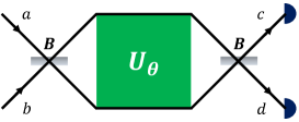
Figure 1: (Color online) Schematic of the standard MZI.

To facilitate our analysis, we focus on the state after the first beam splitter $B|\psi_{{\rm in}}\rangle$, which is called as probe state and denoted by $|\psi\rangle$. We use the basis space spanned by common eigenstates $|j,m\rangle$ of the operators $\hat{\bm{J}}^{2}\!\equiv\!\hat{J}_{x}^{2}+\hat{J}_{y}^{2}+\hat{J}_{z}^{2}$ and $\hat{J}_{z}$ with eigenvalues $j\left(j+1\right)$ and $m$, respectively. An arbitrary pure state $|\psi\rangle$ can be generally expressed as $|\psi\rangle\!=\!\sum_{j}\sum_{m=-j}^{j}C_{j,m}|j,m\rangle$ where $C_{j,m}$ denote the expansion coefficients of $|\psi\rangle$ on $|j,m\rangle$. We here restrict our attention to a family of symmetric pure states with the expansion coefficients satisfying $C_{j,m}\!=\!C_{j,-m}$, suggesting $\langle\hat{J}_{z}\rangle_{\psi}\!=\!0$. Notice that such a family covers a wide range of quantum states as mentioned previously.

According to quantum estimation theory, the QCRB states that, for a given parametric density matrix $\rho_{\theta}$, the phase sensitivity of any unbiased estimator is bounded by $\Delta\theta_{{\rm est}}^{2}\!\leq\![\upsilon F_{Q}(\rho_{\theta})]^{-1}$ where $\upsilon$ is the number of independent measurements and $F_{Q}(\rho_{\theta})$ is the so-called quantum Fisher information (QFI) (Helstrom, 1976; Holevo, 1982; Braunstein and Caves, 1994). In the case as described above, the QFI in terms of the phase-imprinted symmetric pure state $|\psi_{\theta}\rangle\!\equiv\!U_{\theta}|\psi\rangle$ is exactly given by

$$F_{Q}(\psi_{\theta})=4\langle\hat{J}_{z}^{2}\rangle_{\psi}=8\sum_{j}\!\sum_{m=j-\left\lfloor j\right\rfloor}^{j}\!|C_{j,m}|^{2}m^{2},$$ (1)

with $\left\lfloor\thinspace\thinspace\right\rfloor$ denoting the corresponding integer part. Remarkably, the expression in Eq. (1) is irrelevant to the phase parameter $\theta$, meaning that the ultimate sensitivities provided by symmetric pure states do not depend on the true value of the phase shift.

In experiments to achieve the QCRB, one needs to successively perform optimizations over measurements and estimators. A generic optimization procedure is as follows. Consider a general measurement described by a positive-operator-valued measure $\hat{\bm{M}}\!\equiv\!\{\hat{M}_{\chi}\}$ with $\chi$ the results of measurement. Based on $\hat{\bm{M}}$, the accessible phase sensitivity is limited by the inequality $\Delta\theta_{{\rm est}}^{2}\!\leq\![\upsilon F(\rho_{\theta}|\hat{\bm{M}})]^{-1}$, where $F(\rho_{\theta}|\hat{\bm{M}})$ is the classical Fisher information (CFI) defined from below as

$$F(\rho_{\theta}|\hat{\bm{M}})=\sum_{\chi}\frac{1}{p(\chi|\theta)}\bigg{(}\frac{d\,p(\chi|\theta)}{d\theta}\bigg{)}^{2},$$ (2)

with $p(\chi|\theta)\!\equiv\!{\rm Tr}(\hat{M}_{\chi}\rho_{\theta})$ the probability of the outcome $\chi$ conditioned on the specific value of $\theta$. It is well known that such accessible sensitivity bound is achieved by the maximum likelihood estimator for sufficiently large $\upsilon$ with Bayesian estimation methods (Uys and Meystre, 2007; Krischek et al., 2011). Correspondingly, the QCRB can be attained with this interference method by taking a measurement $\hat{\bm{M}}_{{\rm opt}}$ that makes the equality $F(\rho_{\theta}|\hat{\bm{M}}_{{\rm opt}})\!=\!F_{Q}(\rho_{\theta})$ true. $\hat{\bm{M}}_{{\rm opt}}$ thus represents the optimal measurement that we would like to find. In what follows, we clarify that the three conventional measurements as mentioned previously are conditionally optimal for phase estimation in the MZI. We show the optimal conditions by identifying that the quantitative statements of the CFI with respect to the these measurements are equivalent to the expression in Eq. (1).

Conventional measurements.—A TOP particle count measurement is represented as $\hat{\bm{M}}_{{\rm TOP}}\!=\!\{|n_{c},\!n_{d}\rangle\langle n_{c},\!n_{d}|\}$, where the pairs of outcomes $(n_{c},\!n_{d})$ are the number of particles detected at $c$ and $d$ output ports. The conditional probability with respect to $(n_{c},\!n_{d})$ is defined by $p(n_{c},\!n_{d}|\theta)\!=\!|\langle n_{c},\!n_{d}|B^{\dagger}|\psi_{\theta}\rangle|^{2}$. By identifying $2j\!=\!n_{c}\!+\!n_{d}$ and $2\mu\!=\!n_{c}\!-\!n_{d}$, we have $p(n_{c},\!n_{d}|\theta)=p(j,\!\mu|\theta)$, and further obtain

$$p(j,\!\mu|\theta)=\begin{cases}\bigg{|}\sum\limits_{\nu=j-\left\lfloor j\right\rfloor}^{j}\!2\thinspace C_{j,\nu}\cos\!\left(\nu\thinspace\theta\right)d_{\nu,\mu}^{j}\!(\frac{\pi}{2})\bigg{|}^{2},\\ \bigg{|}\sum\limits_{\nu=j-\left\lfloor j\right\rfloor}^{j}\!2\thinspace C_{j,\nu}\sin\!\left(\nu\thinspace\theta\right)d_{\nu,\mu}^{j}\!(\frac{\pi}{2})\bigg{|}^{2},\end{cases}$$ (3)

where the subscript $\mu\!=\!j,j\!-\!2,j\!-\!4,\cdots\thinspace(j\!-\!1,j\!-\!3,j\!-\!5,\cdots)$ in the upper (lower) expression and $d_{\nu,\mu}^{j}\left(\beta\right)\!=\!\langle j,\!\nu|\exp(-i\beta J_{y})|j,\!\mu\rangle$ refers to the Wigner rotation matrix. A direct calculation of the CFI in terms of the TOP measurement with Eq. (3) suggests that the equality $F(\psi_{\theta}|\hat{\bm{M}}_{{\rm TOP}})\!=\!F_{Q}(\psi_{\theta})$ holds when either of the following two conditions is satisfied (see Appendix A): (a) the amplitude coefficients $C_{j,m}$ of $|\psi\rangle$ are real. (b) the true values of $\theta$ are asymptotic to $0$ and $\pi$. This indicates that the TOP measurement is globally optimal in the whole range of parameter value for real-amplitude symmetric pure states and locally optimal at points $\theta\!=\!0$ or $\pi$ for complex-amplitude symmetric pure states (see Table 1). Condition (a) was alternatively obtained in Ref. (Hofmann, 2009), but where there was no statement on condition (b).

Next we consider the SOP particle count measurement, which is denoted by $\hat{\bm{M}}_{{\rm SOP}}\!=\!\{|n_{c}\rangle\langle n_{c}|\}$ in accompany with $n_{c}$ the number of particles counted at $c$ output port. The conditional probability of $n_{c}$ is then given by $p(n_{c}|\theta)\!=\!|\langle n_{c}|B^{\dagger}|\psi_{\theta}\rangle|^{2}$. With the help of the relation $|n_{c}\rangle\langle n_{c}|\!=\!\sum_{n_{d}=0}^{\infty}|n_{c},\!n_{d}\rangle\langle n_{c},\!n_{d}|$, we obtain $p(n_{c}|\theta)\!=\!\sum_{n_{d}=0}^{\infty}p(n_{c},\!n_{d}|\theta).$ By invoking the Cauchy-Schwarz inequality, one can see that $F(\psi_{\theta}|\hat{\bm{M}}_{{\rm TOP}})\!\geq\!F(\psi_{\theta}|\hat{\bm{M}}_{{\rm SOP}})$ (Pezzé and Smerzi, 2013), where the equality holds if and only if

$$\sqrt{p\left(n_{c},\!n_{d}|\theta\right)}=\frac{\lambda}{\sqrt{p\left(n_{c},\!n_{d}|\theta\right)}}\frac{d\,p\left(n_{c},\!n_{d}|\theta\right)}{d\theta},$$ (4)

is satisfied with a nonzero number $\lambda$. Combining Eqs. (3) and (4), we find that the equality $F(\psi_{\theta}|\hat{\bm{M}}_{{\rm SOP}})\!=\!F(\psi_{\theta}|\hat{\bm{M}}_{{\rm TOP}})$ holds only in the asymptotic limits $\theta\!\rightarrow\!0$ and $\pi$. Therefore this indicates that the SOP measurement can attain the QCRB for all symmetric pure states at points $\theta\!=\!0$ and $\pi$ (see Table 1), which is confirmed by a specific example considered in Ref. (Pezzé and Smerzi, 2013).

Table 1: The conditions for achieving the QCRB by three conventional measurements in the MZI. For a specific type of probe state, condition refers to phase interval in which the QCRB is saturated. Here $\mathbb{R}_{{\rm S}}$ and $\mathbb{C}_{{\rm S}}$ denote the sets of real- and complex-amplitude symmetric pure states. Remarkably, for the SOP and TOP measurements, conditions are also satisfied by replacing $|\psi\rangle$ with the corresponding phase averaged mixed states of Eq. (5). In the last row, the remark of $\langle\Delta\hat{N}^{2}\rangle_{\psi}\!=\!0$ means that $|\psi\rangle$ has a definite number of particles.

Measurement	$|\psi\rangle\in\mathbb{R}_{\rm{S}}$	$|\psi\rangle\in\mathbb{C}_{\rm{S}}$	Remark
SOP	$\theta\rightarrow 0,\pi$	$\theta\rightarrow 0,\pi$
TOP	$0\leq\theta\leq\pi$	$\theta\rightarrow 0,\pi$
PD	$0\leq\theta\leq\pi$	$\theta\rightarrow 0,\pi$	$\langle\Delta\hat{N}^{2}\rangle_{\psi}\!=\!0$

Finally, we discuss the PD measurement described by $\hat{\bm{M}}_{{\rm PD}}\!=\!\{|\mu\rangle\langle\mu|\}$, which is also known as the projection measurement with respect to the observable $\hat{J}_{z}$. Notice that the PD measurement is highly related to the TOP measurement, since the latter explicitly reduces to the former when the total particle number of the system is definite. Therefore one can take the PD measurement to saturate the QCRB when the probe state belongs to a subclass of symmetric pure states featuring no fluctuation of particle number, such as, NOON state, twin Fock state. However, the PD measurement fails for the case in which the fluctuating particle number presents, since it is insensitive to distinguish subspaces with different particles numbers. Fortunately, states mostly used in Ramsey interferometer are absence of the fluctuating number of particles. Thus, in such circumstances, the PD measurement is applicable.

Otherwise, in optical interferoemtric setting, quantum states with fluctuating particle number may have coherences between states of different numbers of particles which are generally not measurable (Bartlett et al., 2007; Hyllus et al., 2010; Jarzyna and Demkowicz-Dobrzański, 2012). Now, we consider a general phase averaged state of the form

$$\rho=\int\frac{d\vartheta}{2\pi}\exp\!\big{(}\!-i\vartheta\hat{N}\big{)}\left|\psi\right\rangle\!\left\langle\psi\right|\exp\!\big{(}i\vartheta\hat{N}\big{)},$$ (5)

where $\left|\psi\right\rangle$ of consideration is the symmetric pure state. States in expression of Eq. (5) are vanishing of the coherence of different particle number states as the consequence of the lack of a suitable phase reference frame (Bartlett et al., 2007; Hyllus et al., 2010; Jarzyna and Demkowicz-Dobrzański, 2012). After the MZI process, $\rho$ evolves to $\rho_{\theta}$. A direct calculation of the QFI for $\rho_{\theta}$ yields $F_{Q}(\rho_{\theta})\!=\!F_{Q}(\psi_{\theta})$. Furthermore, by calculating the CFI with respect to the SOP and TOP measurements, we find that the previous important results for pure states can be generalized to mixed states in the form of Eq. (5).

Implementation to Ramsey spectroscopy.—So far we have presented experimentally friendly conditions for saturating the QCRB in a linear MZI. As an example, we apply our results on Ramsey spectroscopy with detection noise. It is well known that a Ramsey spectroscopy (Fig. 2) is formally analogue to the MZI (Fig. 1) by replacing two beam splitters with two Ramsey sequences and phase shift with free evolution. Below we consider a general case of the PD measurement with finite resolution $\sigma$, which is modeled by replacing the ideal probability $p(\mu|\theta)$ with

$$\tilde{p}(\mu|\theta)=\!\!\!\sum_{\mu^{\prime}=-N/2}^{N/2}\!\!\!g(\mu-\mu^{\prime})\,p(\mu^{\prime}|\theta),$$ (6)

where we specify the unbiased Gaussian function $g(\mu\!-\!\mu^{\prime})\!\propto\!\exp[-(\mu\!-\!\mu^{\prime})^{2}/2\sigma^{2}]$ as a resolution function.

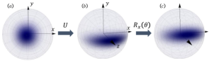
Figure 2: (Color online) Geometric representation of atomic interferometric scheme with the TACT state. Illustrated are Husimi distributions for $N=60$ atoms.

Consider a system of $N$ spin-$1/2$ atoms which we express by the collective angular momentum $\hat{\bm{J}}\!=\!\sum_{i=1}^{N}\hat{\bm{S}}_{i}$ in terms of spin operators $\hat{\bm{S}}_{i}$. The Ramsey interferometric transformation (from Fig. 2(b) to (c)) corresponds to the operation $R_{x}\!\left(\theta\right)\!=\!e^{i\theta\hat{J}_{x}}$ in terms of $\theta=\omega\tau$ with $\omega$ atomic frequency and $\tau$ the interrogation time. We use the two-axis counter-twisted (TACT) state as the input state of Ramsey interferometer. Suppose that the atomic ensemble is initially prepared in a coherent spin state $|\psi_{{\rm c}}\rangle_{z}$, i.e., the fully polarized state along the $z$ axis (Fig. 2(a)). The TACT state is then generated by time evolution under the nonlinear Hamiltonian of $\hat{H}_{{\rm t}}\!=\!\chi(\hat{J}_{x}^{2}-\hat{J}_{y}^{2})$ which is known as the two-axis counter-twisting Hamiltonian (Kitagawa and Ueda, 1993). Several proposals have been presented to simulate this nonlinear Hamiltonian in various physical systems (Liu et al., 2011; Shen and Duan, 2013; Zhang et al., 2014; Huang et al., 2015). Moreover, an additional rotation operation $R_{z}\!\left(\pi/4\right)\!=\!e^{-i\hat{J}_{z}\pi/4}$ is employed to re-orient the squeezing angle of the TACT state so as to acquire the highest degree of sensitivity enhancement. After the compound operation $U\!=\!R_{z}\,U_{t}$, the state of the system becomes (Fig. 2(b))

$$|\psi_{{\rm t}}\rangle_{z}=e^{-i\hat{J}_{z}\pi/4}\,e^{-i\chi t(\hat{J}_{x}^{2}-\hat{J}_{y}^{2})}\,|\psi_{{\rm c}}\rangle_{z}.$$ (7)

By fixing $\chi t\!\sim\!\ln(2\pi N)/2N$ (Kajtoch and Witkowska, 2015), one may expect to acquire a near-Heisenberg scaling limit $\sqrt{\upsilon}\thinspace\Delta\theta\!\sim\!1.24/N$.

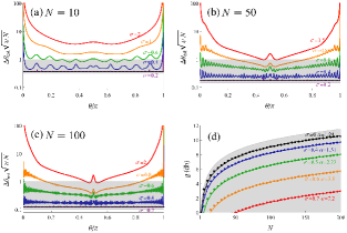
Figure 3: (Color online) Phase sensitivity for the TACT states obtained with a finite-resolution PD measurement (parametrized by $\sigma$). (a-c) The normalized phase sensitivity $\Delta\theta_{{\rm est}}\sqrt{\upsilon N}$ as a function of $\theta$ for the TACT states of different paticle number $N$. Different color curves refer to different values of $\sigma$ and the black-dashed horizontal line corresponds to the ideal case $\sigma=0$. (d) Phase sensitivity gain $g\!\equiv\!-10\log_{10}(\Delta\theta_{{\rm est}}\sqrt{\upsilon N})$ vs $N$ with $\theta\!\sim\!\pi/2N$. Different color filled circles indicate different values of $\sigma$. Solid lines are the results of fitting by $g\!\equiv\!-10\log_{10}(\alpha/\sqrt{N})$ where $\alpha\!=\!1$ corresponds to the Heisenberg-limit-scaling sensitivity gain. The shaded area represents the sub-shot-noise sensitivity region bounded by shot noise limit and Heisenberg limit.

In Fig. 3, we plot the phase sensitivity attained by the finite-resolution PD measurement. For ideal case $\sigma\!=\!0$, as shown in Figs. 3(a-c), the near-Heisenberg scaling sensitivity limit is saturated in the whole phase interval (see Appendix B). According to previous conclusions, this indicates a fact that the probe state here, i.e., $|\psi_{{\rm t}}\rangle_{x}\!=\!e^{-i\hat{J}_{y}\pi/2}\,|\psi_{{\rm t}}\rangle_{z}$, must be a real symmetric pure state. Nevertheless, for the cases in presence of detection noise ($\sigma\!\neq\!0$), the phase sensitivity critically depends on both $\theta$ and $\sigma$. An oscillation with period of $\pi/N$ takes place for small $\sigma$ and disappears for more large values of $\sigma$. Phase interval for sub-shot-noise sensitivity slowly shrinks from the ends of the phase interval towards the middle as $\sigma$ increases. Notably when a small amount of $\sigma$ is present, the phase precision becomes significantly worse at $\theta\!=\!0$ and $\pi$. A similar effect has been found in Refs. (Pezzé and Smerzi, 2013; Lücke et al., 2011). Moreover, it proves that the phase sensitivity becomes more robust against the detection noise by increasing $N$, which is more pronounced in the regime slightly departing from $\pi/2$. In order to examine in detail the roles of the noise power and the size of system on phase sensitivity, we plot in Fig. 3(d) the phase sensitivity gain as a function of $N$ with $\theta\!\sim\!\pi/2N$ corresponding to the first minimum value of the sensitivity in the cases $\sigma\neq 0$, as depicted in Figs. 3(a-c). It is shown that the amount of $g$ increasingly decreases with the increase of $\sigma$, but the rate of degradation does not vary with $N$. This means that for fixed $\sigma$ one can get a higher precision by means of larger number of probes. For instance, in the case $\sigma\!=\!0.7$, a near $3\thinspace{\rm db}$ over the shot noise limit can be acquired for $N\!=\!200$, while no gains obtained for $N\!=\!50$.

In addition, our scheme proves more advantageous than that by means of the one-axis twisted (OAT) state as $|\psi_{{\rm o}}\rangle_{z}\!=\!e^{-i\phi\hat{J}_{z}}\,e^{-i\chi t\hat{J}_{x}^{2}}\,|\psi_{{\rm c}}\rangle_{z}$, where $\phi$ refers to the reorienting angle which rarely depends on the evolution time $t$ (Kitagawa and Ueda, 1993). It was shown that the OAT state would provide a phase sensitivity of $\sqrt{\upsilon}\thinspace\Delta\theta\!\sim\!\sqrt{2}/N$ at a platform time $\chi t\!\sim\!1/\sqrt{N}$ (Pezzé and Smerzi, 2009). Comparing with the OAT scheme, our scheme offers some attractive features in precision atomic spectroscopy, such as fixed reorienting angle, shorter time for creating ideal probe states, and higher measurement sensitivity. More importantly, our scheme can saturate the QCRB in the whole range of the phase shift, while it is only valid at two discrete points $\theta\!=\!0$ and $\pi$ for the OAT case, which is identified by the fact that its corresponding probe state as $|\psi_{{\rm o}}\rangle_{x}\!=\!e^{-i\hat{J}_{y}\pi/2}\,|\psi_{{\rm o}}\rangle_{z}$ be a complex symmetric pure state (Strobel et al., 2014; Gietka et al., 2015).

Conclusion.—We have demonstrated that, under specific conditions, three different conventional detection methods usually implemented in interferometric experiments are able to attain the quantum Cramér-Rao phase sensitivity with a Bayesian statistical method. Interestingly, these conditions are readily met in most of the current experiments on high precision phase measurement. Therefore, this work may have practical impact on gravitational wave detection, atomic clock, and magenetometry and may even be applied for the detection of multipartite entanglement (Strobel et al., 2014; Hauke et al., 2016).

We thank Xiao-Ming Lu for helpful discussions. This work was supported by the NKRDP of China (Grant No. 2016YFA0301803) and the NSFC (Grants No. 91636218). YXH thank the support of the NSF of Zhejiang province through Grants No. LQ16A040001 and the NSFC through Grants No.11605157. XGW also acknowledge the support of the NSFC through Grants No. 11475146.

Appendix A: Analytic solutions of the CFI in terms of the TOP measurement

In this section, we demonstrate in detail that the equality of $F(\psi_{\theta}|\hat{\bm{M}}_{{\rm TOP}})=F_{Q}(\psi_{\theta})$ holds under the following two situations: (a) the expansion coefficients of probe state on $|j,m\rangle$ are real, that is, $|\psi\rangle\in\mathbb{R}_{{\rm S}}$. (b) the true value of the phase is asymptotic to $0$ and $\pi$.

As for the first case, Equation (3) in the main text then reduces to

$$p(j,k|\theta)=\begin{cases}\left[\sum\limits_{\nu=j-\left\lfloor j\right\rfloor}^{j}2\thinspace C_{j,\nu}\cos\left(\nu\thinspace\theta\right)d_{\varsigma,j-k}^{j}\left(\frac{\pi}{2}\right)\right]^{2},&k\thinspace{\rm for}\thinspace{\rm even}\\ \left[\sum\limits_{\nu=j-\left\lfloor j\right\rfloor}^{j}2\thinspace C_{j,\nu}\sin\left(\nu\thinspace\theta\right)d_{\varsigma,j-k}^{j}\left(\frac{\pi}{2}\right)\right]^{2},&k\thinspace{\rm for}\thinspace{\rm odd}\end{cases}$$ (A1)

due to the reality of the amplitude coefficient $C_{j,\nu}$ and of the Wigner rotation matrix $d_{\nu,\mu}^{j}(\frac{\pi}{2})$. Note that the above expressions are also valid when the amplitude coefficient $C_{j,\nu}$ contains a phase factor $e^{i\phi_{j}}$ which only depends on $j$. In this case, we incorporate the phase factor into the basis vector so as to ensure the expansion coefficient remains real. Thus by substituting Eq. (A1) into Eq. (2) in the main text, we obtain

$$F(\psi_{\theta}|\hat{\bm{M}}_{{\rm TOP}}) = \sum_{j}\sum_{k}\frac{1}{p(j,k|\theta)}\bigg{(}\frac{d\,p(j,k|\theta)}{d\theta}\bigg{)}^{2}$$ (A2)

$$= 4\sum_{j}\!\!\sum_{k={\rm even}}\!\left[\!\sum\limits_{\nu=j-\left\lfloor j\right\rfloor}^{j}\!\!2\thinspace C_{j,\nu}\thinspace\nu\thinspace\cos\left(\nu\thinspace\theta\right)d_{\nu,j-k}^{j}\!\left(\frac{\pi}{2}\right)\right]^{2}\!\!+4\sum_{j}\!\!\sum_{k={\rm odd}}\!\left[\!\sum\limits_{\nu=j-\left\lfloor j\right\rfloor}^{j}\!\!2\thinspace C_{j,\nu}\thinspace\nu\thinspace\sin\left(\nu\thinspace\theta\right)d_{\nu,j-k}^{j}\!\left(\frac{\pi}{2}\right)\right]^{2}$$

$$= 8\sum_{j}\sum\limits_{\nu=j-\left\lfloor j\right\rfloor}^{j}C_{j,\nu}^{2}\thinspace\nu^{2}\cos^{2}\left(\nu\thinspace\theta\right)+8\sum_{j}\sum\limits_{\nu=j-\left\lfloor j\right\rfloor}^{j}C_{j,\nu}^{2}\thinspace\nu^{2}\sin^{2}\left(\nu\thinspace\theta\right)$$

$$= 8\sum_{j}\sum\limits_{\nu=j-\left\lfloor j\right\rfloor}^{j}C_{j,\nu}^{2}\thinspace\nu^{2},$$

where the penultimate equality follows from the following identities

$$\sum_{k={\rm even}}d_{\mu,j-k}^{j}\!\left(\frac{\pi}{2}\right)d_{\nu,j-k}^{j}\!\left(\frac{\pi}{2}\right)=\sum_{k={\rm odd}}d_{\mu,j-k}^{j}\!\left(\frac{\pi}{2}\right)d_{\nu,j-k}^{j}\!\left(\frac{\pi}{2}\right)=\frac{1}{2}\thinspace\delta_{\mu,\nu}.$$ (A3)

It can be verified based on the normalization relation of $\langle\psi|B^{\dagger}B|\psi\rangle=1$ associating with $|\psi\rangle$ being a symmetric pure state. This is a key ingredient in obtaining the exact solution of the CFI.

In the second situation, Equation. (3) in the main text can be simplified in the limit $\theta\rightarrow 0$ to

$$p(j,k|\theta)=\begin{cases}\bigg{|}\sum\limits_{\nu=j-\left\lfloor j\right\rfloor}^{j}2\thinspace C_{j,\nu}\,d_{\nu,j-k}^{j}(\frac{\pi}{2})\bigg{|}^{2},&k\thinspace{\rm for}\thinspace{\rm even},\\ \bigg{|}\sum\limits_{\varsigma=j-\left\lfloor j\right\rfloor}^{j}2\thinspace\nu\thinspace\theta\thinspace C_{j,\nu}\,d_{\nu,j-k}^{j}(\frac{\pi}{2})\bigg{|}^{2},&k\thinspace{\rm for}\thinspace{\rm odd},\end{cases}$$ (A4)

by omitting higher order terms with respect to $\theta$. Substituting Eq. (A4) into Eq. (3) in the main text gives

$$F(\psi_{\theta}|\hat{\bm{M}}_{{\rm TOP}}) = \sum_{j}\sum_{k={\rm odd}}\frac{1}{p(j,k|\theta)}\bigg{(}\frac{d\,p(j,k|\theta)}{d\theta}\bigg{)}^{2}$$ (A5)

$$= \sum_{j}\sum_{k={\rm odd}}\frac{\left[\sum\limits_{\mu,\nu=j-\left\lfloor j\right\rfloor}^{j}8\thinspace\mu\thinspace\nu\thinspace\theta\thinspace C_{j,\mu}\thinspace C_{j,\nu}^{\ast}\thinspace d_{j-k,\mu}^{j}\left(\frac{\pi}{2}\right)d_{j-k,\nu}^{j}\left(\frac{\pi}{2}\right)\right]^{2}}{\sum\limits_{\mu,\nu=j-\left\lfloor j\right\rfloor}^{j}4\thinspace\mu\thinspace\nu\thinspace\theta^{2}\thinspace C_{j,\mu}\thinspace C_{j,\nu}^{\ast}\thinspace d_{j-k,\mu}^{j}\left(\frac{\pi}{2}\right)d_{j-k,\nu}^{j}\left(\frac{\pi}{2}\right)}$$

$$= 16\sum_{j}\sum_{k={\rm odd}}\sum\limits_{\mu,\nu=j-\left\lfloor j\right\rfloor}^{j}\mu\thinspace\nu\thinspace C_{j,\mu}\thinspace C_{j,\nu}^{\ast}\thinspace d_{j-k,\mu}^{j}\left(\frac{\pi}{2}\right)d_{j-k,\nu}^{j}\left(\frac{\pi}{2}\right)$$

$$= 8\sum_{j}\sum\limits_{\nu=j-\left\lfloor j\right\rfloor}^{j}\left|C_{j,\nu}\right|^{2}\thinspace\nu^{2},$$

where we have again used Eq. (A3) in the penultimate equality. Following the same procedure, the equality of $F(\psi_{\theta}|\hat{\bm{M}}_{{\rm TOP}})=F_{Q}(\psi_{\theta})$ can be also obtained in the asymptotic limit $\theta\rightarrow\pi$.

Appendix B: Bayesian simulation

In this section, we consider the Bayesian phase estimation protocol. Suppose that $\theta_{0}$ is the true value of phase shift to be estimated for a given parametric density matrix $\rho_{\theta}$ and $p(\chi|\theta)$ represents the conditional probability of the outcome result $\chi$ of $\hat{\bm{M}}$ depending on $\theta$. According to the Bayes theorem, the phase probability distribution is obtained by $p(\theta|\chi)=p(\chi|\theta)\,p(\theta)/p(\chi)$, where $p(\theta)$ is the phase probability distribution prior to the measurement and $p(\chi)$ gives the normalization. After a sequence of $\upsilon$ independent measurements $\hat{\bm{M}}$, the posterior distribution $p(\theta|\left\{\chi_{i}\right\}_{i=1}^{\upsilon})$ of the phase shift $\theta$ conditioned on the measurement outcomes $\left\{\chi_{i}\right\}_{i=1}^{\upsilon}=\chi_{1},\ldots,\chi_{\upsilon}$ is given by

$$p(\theta|\left\{\chi_{i}\right\}_{i=1}^{\upsilon})=\frac{p(\theta)\,\prod_{i=1}^{\upsilon}p(\chi_{i}|\theta)}{\prod_{i=1}^{\upsilon}p(\chi_{i})},$$ (B1)

where the prior knowledge is assumed to be a uniform distribution as $p(\theta)=1$ and the denominator $\prod_{i=1}^{\upsilon}p(\chi_{i})$ serves as the normalization. The estimator $\theta_{{\rm est}}\left(\left\{\chi_{i}\right\}_{i=1}^{\upsilon}\right)$ is chosen as the maximum of the posterior distribution $p(\theta|\left\{\chi_{i}\right\}_{i=1}^{\upsilon})$, which, in the asymptotic limit $\upsilon\rightarrow\infty$, becomes normally distributed centered around the true value $\theta_{0}$ and with variance $\sigma^{2}=1/\upsilon F(\rho_{\theta}|\hat{\bm{M}})$ (Uys and Meystre, 2007; Krischek et al., 2011; Strobel et al., 2014). Thus this estimation scheme can saturate the classical Cramér-Rao lower bound $\Delta\theta_{{\rm est}}^{2}=[\upsilon F(\rho_{\theta}|\hat{\bm{M}})]^{-1}$ in the asymptotic limit of measurements.

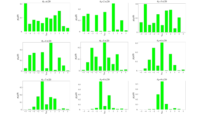
Figure 4: (Color online) Probability distributions $p(\mu|\theta)$ of outcome $\mu$ conditioned on different values of $\theta_{0}$ for the TACT state given by Eq. (7) in the main text. Here $N=10$ and outcomes of the PD measurement $\hat{\bm{M}}_{{\rm PD}}$ are thus $\mu=\left\{0,\,\pm 1,\,\pm 2\,\pm 3\,\pm 4\,\pm 5\right\}$.

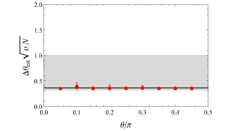
Figure 5: (Color online) Normalized phase sensitivity as a function of the phase shift $\theta$ for the TACT state of particle number $N=10$. The horizontal black line corresponds to the result of the QCRB. Red-filled circles are results of numerical simulations of Bayesian analysis with the number of measurements $\upsilon=100$. The error bars indicate the standard deviation of a single sequence. The black-solid line corresponds to the QCRB limited sensitivity. The shaded area represents the sub-shot-noise sensitivity region bounded by shot noise limit and Heisenberg limit.

Below, we numerically simulate a phase estimation experiment by employing the Bayesian estimation approach and demonstrate that the PD measurement $\hat{\bm{M}}_{{\rm PD}}$ is the optimal in the whole phase interval for achieving the ultimate sensitivity given by the TACT state. Considering the state $|\psi_{{\rm t}}\rangle_{z}$ given in Eq. (7) in the main text and the Ramsey interferometry process $R_{x}\left(\theta\right)$ depicted in Fig. (2) in the main text, the conditional probability with respect to outcomes $\mu$ of the measurement $\hat{\bm{M}}_{{\rm PD}}$ is given by

$$p\left(\mu|\theta\right)=\left|\langle\mu|R_{x}\left(\theta\right)|\psi_{{\rm t}}\rangle_{z}\right|^{2}.$$ (B2)

Here, we set the phase shift to $9$ known values $\theta_{0}/\pi=1/20,\,1/10,\ldots,9/20$. The conditional probabilities for different values of $\theta_{0}$ are plotted in Fig. (4). To simulate the experiment, for each $\theta_{0}$, we randomly draw $5000$ repetitions $\mu_{i}$ of this settings and divided them into sequences of length $\upsilon=100$ for each sequence. Using these outcome results, we implement a Bayesian phase estimation protocol as discussed above. It is known that for sufficiently large $\upsilon$, the phase posterior probability $p(\theta|\left\{\mu_{i}\right\}_{i=1}^{\upsilon})$ becomes a Gaussian distribution. The phase uncertainty is determined by the $68\%$ confidence interval around $\theta_{{\rm est}}$ which corresponds to the maximum of $p(\theta|\left\{\mu_{i}\right\}_{i=1}^{\upsilon})$. As plotted in Fig. (5), we show that the phase sensitivities provided by Bayesian analysis agree with the result obtained from the QCRB.

References

- Caves (1981) C. M. Caves, Phys. Rev. D 23, 1693 (1981).
- Yurke et al. (1986) B. Yurke, S. L. McCall, and J. R. Klauder, Phys. Rev. A 33, 4033 (1986).
- Wineland et al. (1992) D. J. Wineland, J. J. Bollinger, W. M. Itano, F. L. Moore, and D. J. Heinzen, Phys. Rev. A 46, R6797 (1992).
- Holland and Burnett (1993) M. J. Holland and K. Burnett, Phys. Rev. Lett. 71, 1355 (1993).
- Dowling (1998) J. P. Dowling, Phys. Rev. A 57, 4736 (1998).
- Giovannetti et al. (2004) V. Giovannetti, S. Lloyd, and L. Maccone, Science 306, 1330 (2004).
- Giovannetti et al. (2006) V. Giovannetti, S. Lloyd, and L. Maccone, Phys. Rev. Lett. 96, 010401 (2006).
- Giovannetti et al. (2011) V. Giovannetti, S. Lloyd, and L. Maccone, Nat Photon 5, 222 (2011).
- Helstrom (1976) C. W. Helstrom, Quantum Detection and Estimation Theory (Academic, New York, 1976).
- Holevo (1982) A. S. Holevo, Probabilistic and Statistical Aspects of Quantum Theory (North-Holland, Amsterdam, 1982).
- Braunstein and Caves (1994) S. L. Braunstein and C. M. Caves, Phys. Rev. Lett. 72, 3439 (1994).
- Durkin (2010) G. A. Durkin, New J. Phys. 12, 023010 (2010).
- Zhong et al. (2014) W. Zhong, X. M. Lu, X. X. Jing, and X. Wang, J. Phys.A: Math. & Theo. 47, 385304 (2014).
- Zhang et al. (2012) H. Zhang, R. McConnell, S. Ćuk, Q. Lin, M. H. Schleier-Smith, I. D. Leroux, and V. Vuletić, Phys. Rev. Lett. 109, 133603 (2012).
- Hume et al. (2013) D. B. Hume, I. Stroescu, M. Joos, W. Muessel, H. Strobel, and M. K. Oberthaler, Phys. Rev. Lett. 111, 253001 (2013).
- Monras (2006) A. Monras, Phys. Rev. A 73, 033821 (2006).
- Davis et al. (2016) E. Davis, G. Bentsen, and M. Schleier-Smith, Phys. Rev. Lett. 116, 053601 (2016).
- Fröwis et al. (2016) F. Fröwis, P. Sekatski, and W. Dür, Phys. Rev. Lett. 116, 090801 (2016).
- Macrì et al. (2016) T. Macrì, A. Smerzi, and L. Pezzè, Phys. Rev. A 94, 010102 (2016).
- Hofmann (2011) H. F. Hofmann, Phys. Rev. A 83, 022106 (2011).
- Hofmann et al. (2012) H. F. Hofmann, M. E. Goggin, M. P. Almeida, and M. Barbieri, Phys. Rev. A 86, 040102 (2012).
- Pang and Brun (2015) S. Pang and T. A. Brun, Phys. Rev. Lett. 115, 120401 (2015).
- Zhang et al. (2015) L. Zhang, A. Datta, and I. A. Walmsley, Phys. Rev. Lett. 114, 210801 (2015).
- Pezzé and Smerzi (2008) L. Pezzé and A. Smerzi, Phys. Rev. Lett. 100, 073601 (2008).
- Hofmann (2009) H. F. Hofmann, Phys. Rev. A 79, 033822 (2009).
- Pezzé and Smerzi (2013) L. Pezzé and A. Smerzi, Phys. Rev. Lett. 110, 163604 (2013).
- Krischek et al. (2011) R. Krischek, C. Schwemmer, W. Wieczorek, H. Weinfurter, P. Hyllus, L. Pezzé, and A. Smerzi, Phys. Rev. Lett. 107, 080504 (2011).
- Strobel et al. (2014) H. Strobel, W. Muessel, D. Linnemann, T. Zibold, D. B. Hume, L. Pezzè, A. Smerzi, and M. K. Oberthaler, Science 345, 424 (2014).
- Sanders and Milburn (1995) B. C. Sanders and G. J. Milburn, Phys. Rev. Lett. 75, 2944 (1995).
- Berry and Wiseman (2000) D. W. Berry and H. M. Wiseman, Phys. Rev. Lett. 85, 5098 (2000).
- Berry et al. (2009) D. W. Berry, B. L. Higgins, S. D. Bartlett, M. W. Mitchell, G. J. Pryde, and H. M. Wiseman, Phys. Rev. A 80, 052114 (2009).
- Afek et al. (2010) I. Afek, O. Ambar, and Y. Silberberg, Science 328, 879 (2010).
- Joo et al. (2011) J. Joo, W. J. Munro, and T. P. Spiller, Phys. Rev. Lett. 107, 083601 (2011).
- Liu et al. (2013) J. Liu, X. Jing, and X. Wang, Phys. Rev. A 88, 042316 (2013).
- Lang and Caves (2013) M. D. Lang and C. M. Caves, Phys. Rev. Lett. 111, 173601 (2013).
- Anisimov et al. (2010) P. M. Anisimov, G. M. Raterman, A. Chiruvelli, W. N. Plick, S. D. Huver, H. Lee, and J. P. Dowling, Phys. Rev. Lett. 104, 103602 (2010).
- Meyer et al. (2001) V. Meyer, M. A. Rowe, D. Kielpinski, C. A. Sackett, W. M. Itano, C. Monroe, and D. J. Wineland, Phys. Rev. Lett. 86, 5870 (2001).
- Pezzé and Smerzi (2009) L. Pezzé and A. Smerzi, Phys. Rev. Lett. 102, 100401 (2009).
- Bollinger et al. (1996) J. J. . Bollinger, W. M. Itano, D. J. Wineland, and D. J. Heinzen, Phys. Rev. A 54, R4649 (1996).
- Leibfried et al. (2004) D. Leibfried, M. D. Barrett, T. Schaetz, J. Britton, J. Chiaverini, W. M. Itano, J. D. Jost, C. Langer, and D. J. Wineland, Science 304, 1476 (2004).
- Lücke et al. (2011) B. Lücke, M. Scherer, J. Kruse, L. Pezzź, F. Deuretzbacher, P. Hyllus, O. Topic, J. Peise, W. Ertmer, J. Arlt, L. Santos, A. Smerzi, and C. Klempt, Science 334, 773 (2011).
- Bartlett et al. (2007) S. D. Bartlett, T. Rudolph, and R. W. Spekkens, Rev. Mod. Phys. 79, 555 (2007).
- Hyllus et al. (2010) P. Hyllus, L. Pezzé, and A. Smerzi, Phys. Rev. Lett. 105, 120501 (2010).
- Jarzyna and Demkowicz-Dobrzański (2012) M. Jarzyna and R. Demkowicz-Dobrzański, Phys. Rev. A 85, 011801 (2012).
- Uys and Meystre (2007) H. Uys and P. Meystre, Phys. Rev. A 76, 013804 (2007).
- Kitagawa and Ueda (1993) M. Kitagawa and M. Ueda, Phys. Rev. A 47, 5138 (1993).
- Liu et al. (2011) Y. C. Liu, Z. F. Xu, G. R. Jin, and L. You, Phys. Rev. Lett. 107, 013601 (2011).
- Shen and Duan (2013) C. Shen and L.-M. Duan, Phys. Rev. A 87, 051801 (2013).
- Zhang et al. (2014) J.-Y. Zhang, X.-F. Zhou, G.-C. Guo, and Z.-W. Zhou, Phys. Rev. A 90, 013604 (2014).
- Huang et al. (2015) W. Huang, Y.-L. Zhang, C.-L. Zou, X.-B. Zou, and G.-C. Guo, Phys. Rev. A 91, 043642 (2015).
- Kajtoch and Witkowska (2015) D. Kajtoch and E. Witkowska, Phys. Rev. A 92, 013623 (2015).
- Gietka et al. (2015) K. Gietka, P. Szańkowski, T. Wasak, and J. Chwedeńczuk, Phys. Rev. A 92, 043622 (2015).
- Hauke et al. (2016) P. Hauke, M. Heyl, L. Tagliacozzo, and P. Zoller, Nat Phys 12, 778 (2016).