$6\pi$ Josephson effect in Majorana box devices

Abstract

We study Majorana devices featuring a competition between superconductivity and multi-channel Kondo physics. Our proposal extends previous work on single-channel Kondo systems to a topologically nontrivial setting of non-Fermi liquid type, where topological superconductor wires (with gap $\Delta$) represent leads tunnel-coupled to a Coulomb-blockaded Majorana box. On the box, a spin degree of freedom with Kondo temperature $T_{K}$ is nonlocally defined in terms of Majorana states. For $\Delta\gg T_{K}$, the destruction of Kondo screening by superconductivity implies a $4\pi$-periodic Josephson current-phase relation. Using a strong-coupling analysis in the opposite regime $\Delta\ll T_{K}$, we find a $6\pi$-periodic Josephson relation for three leads, with critical current $I_{c}\approx e\Delta^{2}/\hbar T_{K}$, corresponding to the transfer of fractionalized charges $e^{*}=2e/3$.

Introduction.—An important goal of condensed matter physics and quantum information science is to implement, thoroughly understand, and usefully employ systems hosting topologically protected Majorana bound states (MBSs) Alicea2012 ; Leijnse2012 ; Beenakker2013 . These states are expected near the ends of topological superconductor (TS) wires, and experimental evidence for MBSs has been reported for semiconductor-superconductor heterostructures with proximitized InAs or InSb nanowires Mourik2012 ; Krogstrup2015 ; Higginbotham2015 ; Albrecht2016 ; Leo2016 . For a Coulomb-blockaded superconducting island containing more than two MBSs (‘Majorana box’), a spin operator is encoded by pairs of spatially separated MBSs. When normal leads are coupled to the MBSs, this spin is screened through cotunneling processes, culminating in the so-called topological Kondo effect (TKE) Beri2012 ; Altland2013 ; Beri2013 ; Crampe2013 ; Tsvelik2013 ; Zazunov2014 ; Altland2014 ; Eriksson2014 ; Galpin2014 ; Buccheri2015 ; Buccheri2016 ; Giuliano2016a ; Giuliano2016b which exhibits non-Fermi liquid physics below $T_{K}$. Unlike other overscreened multi-channel Kondo systems Gogolin1998 ; Potok2007 ; Pierre2015 ; Keller2015 , the TKE is intrinsically stable against anisotropies. Majorana devices could thus realize multi-channel Kondo effects without delicate fine tuning of parameters.

We here study the Josephson effect for a Majorana box with superconducting (instead of normal) leads as illustrated in Fig. 1. Previous theoretical work for Majorana systems contacted by superconducting electrodes has only addressed cases without TKE Zazunov2012 ; Peng2015 ; Ioselevich2016 ; Zazunov2016 ; Setiawan2016 . In our setup, a nontrivial competition between superconductivity and the Kondo effect arises because lead states below the superconducting gap $\Delta$ are not available anymore for screening the box spin. The simpler single-channel spin-$1/2$ Kondo case, which is of Fermi-liquid type and can be realized when two superconducting leads are connected to a quantum dot Alvaro2011 , was studied in detail both theoretically Glazman1989 ; Golub1996 ; Rozhkov1999 ; Vecino2003 ; Siano2004 ; Choi2004 ; Karrasch2008 ; Luitz2012 and experimentally Kasumov1999 ; VanDam2006 ; Cleuziou2006 ; Jorgensen2007 ; Eichler2009 ; Delagrange2015 . It has been established that a local quantum phase transition at $\Delta/T_{K}\simeq 1$ separates a so-called 0-phase (small $\Delta/T_{K}$) and a $\pi$-phase (large $\Delta/T_{K}$), where essentially the entire crossover is described by universal scaling functions of $\Delta/T_{K}$. Deep in the 0-phase, the Kondo resonance persists and yields the current-phase relation of a fully transparent superconducting junction, while in the $\pi$-phase the Kondo effect is almost completely quenched and one finds a negative supercurrent.

With the Majorana device proposed below, the rich interplay between superconductivity and multi-channel Kondo screening may also become experimentally accessible. The symmetry group of the TKE is here affected by even a tiny gap $\Delta$ due to the proliferation of crossed Andreev reflection processes. For $\Delta\ll T_{K}$ and $M=3$ attached leads, our nonperturbative strong-coupling theory predicts that two-channel Kondo physics is responsible for a $6\pi$-periodic Josephson effect with critical current $I_{c}\approx e\Delta^{2}/\hbar T_{K}$. This periodicity implies charge fractionalization in units of $e^{*}=2e/3$ for elementary transfer processes. On the other hand, for $\Delta\gg T_{K}$, we recover the well-known $4\pi$-periodic current-phase relation of parity-conserving topological Josephson junctions Alicea2012 ; Leijnse2012 ; Beenakker2013 . In view of the rapid experimental progress on Majorana states in semiconductor-superconductor devices Mourik2012 ; Krogstrup2015 ; Higginbotham2015 ; Albrecht2016 ; Leo2016 , our predictions can likely be tested soon, e.g., by the techniques recently employed to observe the $4\pi$ Josephson effect Bocquillon2016 .

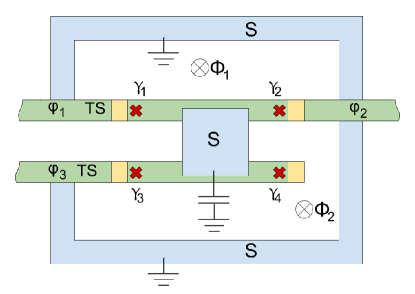
Figure 1: Schematic device setup with $M=3$ superconducting leads, using two long parallel InAs (or InSb) nanowires. Proximitized parts give TS wire regions (green) with Majorana end states (red crosses, shown only on the parts forming the Majorana box). Short non-proximitized sections (yellow) are used as gate-tunable tunnel contacts. The floating Majorana box with four MBSs ($\gamma_{j}$) is created by joining the two central TS parts through an $s$-wave superconducting bridge (blue). Superconducting leads are obtained from outer TS wire sections in contact with conventional superconductors (blue). By tuning magnetic fluxes ($\Phi_{1,2}$), the supercurrents $I_{j}$ can be studied as function of the phases $(\varphi_{1},\varphi_{2},\varphi_{3})$.

Model.—The superconducting leads attached to the Majorana box are described as semi-infinite TS wires of symmetry class $D$. For $M$ leads, the effectively spinless low-energy Hamiltonian is (we put $e=\hbar=v_{F}=1$) Alicea2012

$$H_{\rm leads}=\sum_{j=1}^{M}\int_{0}^{\infty}dx\Psi^{\dagger}_{j}(x)\left[-i\partial_{x}\sigma_{z}+\Delta_{j}e^{-i\varphi_{j}\sigma_{z}}\sigma_{y}\right]\Psi_{j}(x),$$ (1)

where $\Delta_{j}$ denotes the absolute value and $\varphi_{j}$ the phase of the respective proximity-induced superconducting gap, Pauli matrices $\sigma_{x,y,z}$ and unity $\sigma_{0}$ act in Nambu space, and the spinors $\Psi_{j}=(\psi_{j,R},\psi_{j,L}^{\dagger})^{T}$ are expressed in terms of right/left-moving fermion operators with boundary condition $\psi_{j,R}(0)=\psi_{j,L}(0)$. We mainly discuss results for identical gaps, $\Delta_{j}=\Delta$, but our theory applies to the general case SM1 . The reason why we did not assume conventional $s$-wave superconductors as leads is that different pairing symmetries for the box and the leads imply a supercurrent blockade Zazunov2012 , where only above-gap quasiparticle transport is possible under rather general conditions Peng2015 ; Ioselevich2016 ; Zazunov2016 ; Setiawan2016 . Fortunately, leads with effective $p$-wave pairing symmetry may be implemented in a natural way, see below and Fig. 1. At $x=0$, each lead fermion $\psi_{j}$ is then coupled by a tunnel amplitude $t_{j}$ to the respective Majorana operator $\gamma_{j}=\gamma_{j}^{\dagger}$ on the box, with anticommutator $\{\gamma_{j},\gamma_{k}\}=\delta_{jk}$. We study energy scales well below the proximity gap $\Delta_{\rm box}$ on the box, where $\Delta_{\rm box}$ and $\Delta\lesssim\Delta_{\rm box}$ are taken as independent parameters and above-gap quasiparticles on the box are neglected. For a large charging energy $E_{C}$, charge quantization implies a parity constraint for the Majorana states on the box and tends to suppress quasiparticle poisoning processes. Nonetheless, the ground state remains degenerate for $M>2$, where the Majorana bilinears $i\gamma_{j}\gamma_{k}$ represent the box spin Beri2012 ; Altland2014 . The projection to the Hilbert space sector with quantized box charge yields Beri2012

$$H_{\rm EC}=\sum_{j\neq k}^{M}\lambda_{jk}\psi^{\dagger}_{j}(0)\psi_{k}(0)\gamma_{k}\gamma_{j},$$ (2)

where the dimensionless exchange couplings $\lambda_{jk}=2t_{j}t^{\ast}_{k}/E_{C}$ describe elastic cotunneling between leads $j\leftrightarrow k$. For $\Delta=0$, Refs. Beri2012 ; Altland2013 ; Beri2013 show that $H_{\rm leads}+H_{\rm EC}$ gives a TKE of SO${}_{2}(M)$ symmetry with

$$T_{K}=E_{C}e^{-\pi/[2(M-2)\bar{\lambda}]},\quad\bar{\lambda}=\frac{1}{M(M-1)}\sum_{j\neq k}\lambda_{jk},$$ (3)

where the group relation SO${}_{2}(3)\sim$ SU${}_{4}(2)$ implies a four-channel Kondo effect for $M=3$ Fabrizio1994 . For $\Delta\neq 0$, the competition between Kondo physics and superconductivity is then controlled by the ratio $\Delta/T_{K}$. For $\varphi_{j}=0$, the above model also describes junctions of off-critical anisotropic spin chains Crampe2013 ; Tsvelik2013 ; Giuliano2016a ; Giuliano2016b .

Implementation.—Before turning to results, we briefly discuss how to realize this model for the simplest nontrivial case $M=3$, cf. Fig. 1. The floating box is defined by connecting two parallel TS wires by an $s$-wave superconductor. Nanowires can be fabricated with an epitaxial superconducting shell Krogstrup2015 , where a magnetic field simultaneously drives both wires into the TS phase Alicea2012 . We assume that the TS sections on the box are so long that overlap between different Majorana states is negligible. Non-proximitized wire parts yield gate-tunable tunnel barriers, and leads are defined by the outer TS wires in Fig. 1. Using available Majorana wires Albrecht2016 , it appears possible to realize the Kondo regime Beri2012 ; Zazunov2014 ; Altland2014 ; Beri2016 . In a loop geometry with magnetic fluxes Giazotto , one can change the phase differences between TS leads and measure the current-phase relation.

Josephson current.—It is often convenient to integrate out the lead fermion modes away from $x=0$. The Euclidean action, $S=S_{\rm leads}+S_{\rm box}+S_{\rm EC}$, is thereby expressed in terms of Majorana fields $\gamma_{j}(\tau)$ and boundary ($x=0$) Grassmann-Nambu spinor fields, $\Psi_{j}(\tau)=\left(\psi_{j},\bar{\psi}_{j}\right)^{T}$. With inverse temperature $\beta$, $H_{\rm leads}$ gives

$$S_{\rm leads}=-\frac{1}{2}\int_{0}^{\beta}d\tau d\tau^{\prime}\sum_{j}\bar{\Psi}_{j}(\tau)G^{-1}_{j}(\tau-\tau^{\prime})\Psi_{j}(\tau^{\prime}),$$ (4)

where the boundary Green’s function $G_{j}(\tau)$ has the Fourier transform Zazunov2016

$$G_{j}(\omega)=-i\ {\rm sgn}(\omega)\sqrt{1+\frac{\Delta_{j}^{2}}{\omega^{2}}}\ \sigma_{0}+\frac{\Delta_{j}e^{-i\varphi_{j}\sigma_{z}}}{i\omega}\sigma_{x}.$$ (5)

The box action is $S_{\rm box}=\frac{1}{2}\int d\tau\sum_{j}\gamma_{j}\partial_{\tau}\gamma_{j}$, and $S_{\rm EC}=\int d\tau H_{\rm EC}(\tau)$. Expressing the partition function as functional integral, $Z=e^{-\beta F}=\int{\cal D}(\Psi_{j},\gamma_{j})e^{-S}$, the supercurrent $I_{j}$ through lead no. $j$ (oriented towards the box) follows as phase derivative of the free energy, $I_{j}=(2e/\hbar)\partial_{\varphi_{j}}F,$ where current conservation implies $\sum_{j}I_{j}=0$. We discuss the zero-temperature limit in what follows.

Atomic limit: $\Delta\gg T_{K}$.—In the atomic limit, after gauging out the $\varphi_{j}$ phases from the bulk, Eq. (5) simplifies to $G_{j}(\omega)\simeq\frac{\Delta_{j}}{i\omega}(\sigma_{0}+\sigma_{x})$. As a consequence, the lead action (S2) becomes $S_{\rm leads}\simeq\frac{1}{2}\sum_{j}\int d\tau\ \eta_{j}\partial_{\tau}\eta_{j}$, where the boundary fermions define zero-energy Majorana operators, $\eta_{j}=(\psi_{j}+\psi_{j}^{\dagger})/\sqrt{2\Delta_{j}}$, and Eq. (2) yields the effective low-energy Hamiltonian $H_{\rm eff}=\frac{1}{2}\sum_{j\neq k}\sqrt{\Delta_{j}\Delta_{k}}\lambda_{jk}e^{i(\varphi_{j}-\varphi_{k})/2}\eta_{j}\eta_{k}\gamma_{k}\gamma_{j}.$ Since all mutually commuting products $2i\eta_{j}\gamma_{j}=\sigma_{j}=\pm 1$ are conserved, we arrive at the $4\pi$-periodic supercurrents

$$I_{j}=\frac{e\Delta}{\hbar}\sum_{k\neq j}\lambda_{jk}\sigma_{j}\sigma_{k}\sin\left(\frac{\varphi_{j}-\varphi_{k}}{2}\right),$$ (6)

where the $\{\sigma_{j}\}$ correspond to different fermion parity sectors and we put $\Delta_{j}=\Delta$. The Kondo effect is suppressed in the atomic limit since no low-energy quasiparticles in the leads are available to screen the box spin. In fact, Eq. (6) also describes topological Josephson junctions with featureless tunnel contacts Alicea2012 .

Renormalization group (RG) analysis.—To tackle the case of arbitrary $\Delta/T_{K}$, we start with the one-loop RG equations. Renormalizations appear for $\Delta$, for the $\lambda_{jk}$, and for the complex-valued crossed Andreev reflection amplitudes $\kappa_{jk}=\kappa_{kj}$ (with $j\neq k$). Such couplings are absent in the bare model but will be generated during the RG flow by an interplay of exchange processes ($\lambda$) and superconductivity ($\Delta$). They describe the creation (or annihilation) of two fermions in different leads by splitting (or forming) a Cooper pair on another lead, corresponding to the additional term

$$H_{\rm CAR}=\sum_{j<k}\kappa_{jk}\psi_{j}^{\dagger}(0)\psi_{k}^{\dagger}(0)\gamma_{k}\gamma_{j}+{\rm h.c.}$$ (7)

In the Supplementary Material SM1 , we provide a derivation of the RG equations for arbitrary $\Delta_{j}\ll D$, where the bandwidth is $D\simeq{\rm min}(E_{C},\Delta_{\rm box})$. For $\Delta_{j}=\Delta$, taking a gauge where the phase dependence only appears in $H_{\rm EC}+H_{\rm CAR}$, we obtain ($j\neq k$)

$$\frac{d\lambda_{jk}}{d\ell} = \frac{2}{\pi}\sum_{m\neq(j,k)}^{M}\Bigl{[}\sqrt{1+\delta^{2}}\left(\lambda_{jm}\lambda_{mk}+\kappa_{jm}\kappa_{mk}^{\ast}\right)$$ (8)

$$+ \delta\left(\lambda_{jm}\kappa_{mk}^{\ast}+\kappa_{jm}\lambda_{mk}\right)\Bigr{]},$$

$$\frac{d\kappa_{jk}}{d\ell} = \frac{2}{\pi}\sum_{m\neq(j,k)}^{M}\Bigl{[}\delta\left(\lambda_{jm}\lambda_{mk}^{\ast}+\kappa_{jm}\kappa_{mk}\right)$$

$$+ \sqrt{1+\delta^{2}}\left(\lambda_{jm}\kappa_{mk}+\kappa_{jm}\lambda_{mk}^{\ast}\right)\Bigr{]},$$

with $\delta(\ell)=e^{\ell}\Delta/D$ and initial conditions $\kappa_{jk}(0)=0$ and $\lambda_{jk}(0)=(2t_{j}t^{*}_{k}/E_{C})e^{i(\varphi_{j}-\varphi_{k})/2}$. The RG flow thus only depends on the gauge-invariant phase differences $\varphi_{j}-\varphi_{k}$.

RG solution for the unbiased case.—Putting all $\varphi_{j}=0$, the above RG equations can be solved analytically. The matrices $\Lambda_{jk}^{(\pm)}=\lambda_{jk}\pm\kappa_{jk}$ may now be chosen real symmetric and obey decoupled flow equations,

$$\frac{d\Lambda^{(\pm)}_{jk}}{d\ell}=\frac{2}{\pi}(\sqrt{1+\delta^{2}}\pm\delta)\sum_{m\neq(j,k)}^{M}\Lambda_{jm}^{(\pm)}\Lambda_{mk}^{(\pm)},$$ (9)

which (up to a rescaling) coincide with those for the TKE. The results of Refs. Beri2012 ; Altland2013 ; Beri2013 ; Zazunov2014 imply that anisotropies in the $\Lambda_{jk}^{(\pm)}$ are irrelevant perturbations, and both matrices scale towards isotropy, $\Lambda^{(\pm)}_{jk}(\ell)\to\Lambda_{\pm}(\ell)[1-\delta_{jk}]$. For an isotropic initial condition, $\Lambda_{\pm}(0)=\bar{\lambda}$, with the average coupling $\bar{\lambda}$ in Eq. (3), we find from Eq. (9)

$$\Lambda_{\pm}(\ell)=\lambda(\ell)\pm\kappa(\ell)=\frac{\bar{\lambda}}{1-\frac{2(M-2)\bar{\lambda}}{\pi}{\cal F}_{\pm}(\ell)},$$ (10)

with the monotonically increasing functions

$${\cal F}_{\pm}(\ell)=\left[\sqrt{1+\delta^{2}}+\ln\sqrt{\frac{\sqrt{1+\delta^{2}}-1}{\sqrt{1+\delta^{2}}+1}}\pm\delta\right]^{\delta(\ell)}_{\delta(0)}.$$ (11)

Hence $\Lambda_{\pm}(\ell)$ as well as $\delta(\ell)$ scale towards strong coupling (with $\Lambda_{+}>\Lambda_{-}$). For $\Delta\ll T_{K}$ with $T_{K}$ in Eq. (3), the energy scales $T_{\pm}$ where $\Lambda_{\pm}(\ell)$ enters the strong-coupling regime can be estimated as $T_{\pm}\simeq T_{K}e^{\pm\frac{\pi\Delta}{2(M-2)\bar{\lambda}E_{C}}}$. The renormalized couplings $\lambda\gtrsim\kappa$ are then of order unity when reaching the strong-coupling regime. Now any finite coupling $\kappa$ (as well as $\Delta$) is expected to destabilize the SO${}_{2}(M)$ Kondo fixed point and to induce a flow to a stable fixed point with symmetry group SO${}_{1}(M)$. For $M=3$, this has been shown in Ref. Giuliano2016a , where the relation SO${}_{1}(3)\sim$ SU${}_{2}(2)$ implies a two-channel (instead of the $\Delta=0$ four-channel Beri2012 ; Fabrizio1994 ) Kondo fixed point. On the other hand, for $\Delta\gg T_{K}$, the pairing variable $\delta(\ell)$ reaches the strong-coupling regime first and we are back to the atomic limit. In the remainder, we discuss the limit $\Delta\ll T_{K}$ for $M=3$ leads.

Phase-biased case.—For $\varphi_{j}\neq 0$, the RG equations (S14) are more difficult to solve. Numerical analysis of Eq. (S14) shows that for $\Delta\ll T_{K}$, the absolute values of the couplings $\lambda_{jk}$ and $\kappa_{jk}$ again flow towards isotropy but with a specific phase dependence. With the real positive couplings $\lambda(\ell)$ and $\kappa(\ell)$ in Eq. (10), we find $\lambda_{jk}(\ell)\to\lambda(\ell)e^{i(\varphi_{j}-\varphi_{k})/2}$ and $\kappa_{jk}(\ell)\to\kappa(\ell)e^{i\theta_{jk}}$ as one approaches the strong-coupling regime, where $\theta_{jk}=(\varphi_{j}+\varphi_{k})/2-\varphi_{0}$ with the center-of-mass phase $\varphi_{0}=(\varphi_{1}+\varphi_{2}+\varphi_{3})/3$. This result for $\theta_{jk}$ follows directly from gauge invariance and a stationarity condition SM1 . Finally, in what follows, it is convenient to remove the phase factors from $H_{\rm EC}+H_{\rm CAR}$ by the gauge transformation $\psi_{j,R/L}(x)\to e^{i(\varphi_{j}-\varphi_{0})/2}\psi_{j,R/L}(x)$.

Strong-coupling analysis for $M=3$ and $\Delta\ll T_{K}$.—We now turn to the asymptotic low-energy regime which can be accessed by perturbation theory around the two-channel Kondo fixed point Eriksson2014 ; Affleck1993 ; Coleman1995 . We first introduce chiral fermion fields for the TS leads by an unfolding transformation, $\Phi_{j}(x>0)=\psi_{j,R}(x)$ and $\Phi_{j}(x<0)=\psi_{j,L}(-x)$, and switch to their Majorana representations, $\Phi_{j}(x)=[\eta_{j}(x)+i\xi_{j}(x)]/\sqrt{2}$. Using the renormalized couplings $\Lambda_{\pm}=\lambda\pm\kappa$ in Eq. (10) with $\Lambda_{+}\gg\Lambda_{-}$, we then obtain

$$H_{\rm EC}+H_{\rm CAR}=\Lambda_{+}{\bf S}\cdot{\bf S}_{\eta}+\Lambda_{-}{\bf S}\cdot{\bf S}_{\xi},$$ (12)

where we define the spin-$1/2$ operators ${\bf S}=-\frac{i}{2}{\bm{\gamma}}\times{\bm{\gamma}}$, ${\bf S}_{\eta}=-\frac{i}{2}{\bm{\eta}}(0)\times{\bm{\eta}}(0)$, and ${\bf S}_{\xi}=-\frac{i}{2}{\bm{\xi}}(0)\times{\bm{\xi}}(0)$, with ${\bm{\gamma}}=(\gamma_{1},\gamma_{2},\gamma_{3})^{T}$ and similarly for the ${\bm{\eta}}$ and ${\bm{\xi}}$ Majorana triplets. The theory for $\Delta=\Lambda_{-}=0$ then describes the two-channel Kondo problem. The strong-coupling regime is accessible by employing the following rules Eriksson2014 ; Affleck1993 ; Coleman1995 : (i) Screening processes leading to a singlet state between ${\bm{S}}$ and ${\bm{S}}_{\eta}$ imply the replacement ${\bm{S}}\to iT_{K}^{-1/2}\gamma_{0}{\bm{\eta}}(0)$, where the Majorana operator $\gamma_{0}$ describes the residual unscreened spin. With time ordering ${\cal T}$, we have $\langle{\cal T}\gamma_{0}(\tau)\gamma_{0}(0)\rangle=\frac{1}{2}{\rm sgn}(\tau)$. (ii) The Majorana triplet ${\bm{\eta}}(x)$ obeys twisted boundary conditions, ${\bm{\eta}}(x)\to{\rm sgn}(x){\bm{\eta}}(x)$, while the ${\bm{\xi}}$ triplet remains unchanged. In terms of fermions, this implies perfect Andreev reflection, $\psi_{j,R}(0)=-\psi^{\dagger}_{j,L}(0)$. (iii) For $\Delta=\Lambda_{-}=0$, the leading irrelevant operator is given by $H_{\rm LIO}=2\pi T_{K}^{-1/2}\gamma_{0}\eta_{1}(0)\eta_{2}(0)\eta_{3}(0)$, with scaling dimension $d=3/2$. The perturbation $H_{-}$ due to $\Lambda_{-}$, see Eq. (12), is then also irrelevant with $d=3/2$.

We now have to include the bulk pairing term $\propto\Delta$ in the leads in a nonperturbative manner. In fact, the leading contribution to $I_{j}$ follows from second-order perturbation theory in $H^{\prime}=H_{\rm LIO}+H_{-}$. Since $H^{\prime}$ has scaling dimension $d=3/2$, one naively expects a linear temperature $(T$) dependence of $I_{j}$. However, $\Delta$ is RG-relevant and provides a $1/T$ factor, resulting in a finite supercurrent at $T=0$. We then need the boundary Green’s functions for the field combinations $[\psi_{j,R}(0)-\psi_{j,L}^{\dagger}(0)]/\sqrt{2}$ representing decoupled TS leads with twisted boundary conditions. Following the steps in Ref. Zazunov2016 , we thereby obtain the lead Majorana correlation functions at the boundary ($x=0^{+}$),

$$\langle{\cal T}\eta_{j}(\tau)\xi_{k}(0)\rangle=-i\delta_{jk}\Delta\cos(\varphi_{j}-\varphi_{0})f(\tau),$$ (13)

$$\langle{\cal T}\eta_{j}(\tau)\eta_{k}(0)\rangle=\langle{\cal T}\xi_{j}(\tau)\xi_{k}(0)\rangle=-\delta_{jk}\partial_{\tau}f(\tau),$$

$$f(\tau)=\int\frac{d\omega}{2\pi}\frac{1-e^{-\sqrt{\omega^{2}+\Delta^{2}}/T_{K}}}{\sqrt{\omega^{2}+\Delta^{2}}}\cos(\omega\tau).$$

The $T=0$ supercurrents $I_{j}$ then come from the second-order contribution to the free energy, $F^{(2)}=-\frac{1}{2}\int d\tau\langle{\cal T}H^{\prime}(\tau)H^{\prime}(0)\rangle$. Using Eq. (13) and Wick’s theorem SM1 , the phase derivatives of $F^{(2)}$ yield

$$I_{j}(\varphi_{1},\varphi_{2},\varphi_{3})=I_{0}\sum_{k\neq j}^{3}\Biggl{(}\sin(\varphi_{j}-\varphi_{k})$$ (14)

$$+\frac{1}{3}\sin\left(\frac{\varphi_{j}+\varphi_{k}-2\varphi_{p}}{3}\right)-\frac{1}{3}\sin\left(\frac{\varphi_{k}+\varphi_{p}-2\varphi_{j}}{3}\right)\Biggr{)},$$

where $p\neq(j,k)$. The current scale, and thus ultimately the critical current $I_{c}$, is set by

$$I_{0}=\zeta\frac{\Delta}{T_{K}}\frac{e\Delta}{\hbar},\quad\zeta=\frac{\Lambda_{-}(\Lambda_{-}-2\pi)}{3}f^{3}(0).$$ (15)

The dimensionless number $\zeta$ is of order unity and can be positive or negative. Compared to the conventional Kondo system with critical current $I_{c}=e\Delta/\hbar$ Glazman1989 , there is a suppression factor $\Delta/T_{K}\ll 1$ due to the residual unscreened spin encoded by $\gamma_{0}$. Equation (14) obeys current conservation, $\sum_{j}I_{j}=0$, and predicts a $6\pi$-periodic phase dependence which in turn implies charge fractionalization in units of $e^{*}=2e/3$ for charge transfer between TS leads. For finite $\Delta$, we have a two-channel instead of a four-channel Kondo problem, and hence this value of $e^{*}$ differs from the one for normal leads probed by shot noise Zazunov2014 ; Beri2016 . The $6\pi$ periodicity is due to the non-Fermi liquid nature of the two-channel Kondo fixed point and can be seen explicitly by putting $(\varphi_{1},\varphi_{2},\varphi_{3})=(\varphi,\varphi,0)$, where Eq. (14) gives $I_{1,2}/I_{0}=\sin\varphi+[\sin(\varphi/3)+\sin(2\varphi/3)]/3$. On the other hand, for $(\varphi_{1},\varphi_{2},\varphi_{3})=(\varphi/2,-\varphi/2,0)$, one gets a $4\pi$ periodicity, $I_{1,2}/I_{0}=\pm[\sin(\varphi)+2\sin(\varphi/2)]$, since the third terminal is now basically decoupled ($I_{3}=0$). In general, the $6\pi$ periodicity coexists with $2\pi$ and $4\pi$ effects. Finally, we note that for an observation of the $6\pi$ Josephson effect, one should probe the supercurrent at finite frequencies, cf. Ref. Bocquillon2016 .

Conclusions.—We have studied the Josephson effect through a multi-channel Kondo impurity. This problem could be realized using a Majorana box device with superconducting leads. The different periodicities in the atomic and the strong-coupling limit ($4\pi$ vs $6\pi$ for three leads) could indicate a quantum phase transition at $\Delta\approx T_{K}$. This point requires a detailed numerical study which can also clarify to what extent the crossover is universal in $\Delta/T_{K}$. It would also be interesting to study topologically trivial $p$-wave superconductors as leads, and to generalize our strong-coupling analysis to $M>3$ where one may encounter even higher periodicities in the current-phase relation.

Supplementary Material: $\bm{6\pi}$ Josephson effect in Majorana box devices

We here provide a detailed derivation of the RG equations and further discuss the strong-coupling solution described in the main text.

.1 Derivation of RG equations

In this part, we present a derivation of the RG equations, allowing for anisotropies in the gap values $\Delta_{j}$. Our approach holds for arbitrary $\Delta_{j}\ll D$, where $D$ denotes an effective bandwidth for the bulk fermions encapsulated by the boundary fields $\psi_{j}$. We first derive the one-loop RG equations without fixing a gauge, and then choose a convenient gauge where the RG equations depend on the phases $\varphi_{j}$ only through initial conditions. Eventually, the Josephson current-phase relation are expressed in terms of gauge-invariant phase differences $\varphi_{j}-\varphi_{k}$, where charge conservation requires that the action

$$S[\{\psi_{j},\gamma_{j}\}]=S_{\rm leads}+S_{\rm box}+S_{\rm EC}+S_{\rm CAR}$$ (S1)

is invariant under a global (time- and $j$-independent) gauge transformation, $\psi_{j}\to e^{i\theta}\psi_{j}$ and $\varphi_{j}\to\varphi_{j}-2\theta$, with arbitrary phase $\theta$.

The leads are described by [cf. Eqs. (4) and (5) in the main text]

$$S_{\rm leads} = -\frac{1}{2}\int_{0}^{\beta}d\tau d\tau^{\prime}\sum_{j}\bar{\Psi}_{j}(\tau)G^{-1}_{j}(\tau-\tau^{\prime})\Psi_{j}(\tau^{\prime}),$$

$$G_{j}(\omega) = -i\ {\rm sgn}(\omega)\sqrt{1+\frac{\Delta_{j}^{2}}{\omega^{2}}}\ \sigma_{0}+\frac{\Delta_{j}e^{-i\varphi_{j}\sigma_{z}}}{i\omega}\sigma_{x},$$ (S2)

with the boundary Grassmann fields $\psi_{j}(\tau)$ and $\bar{\psi}_{j}(\tau)$ determining the Nambu spinor $\Psi_{j}(\tau)=(\psi_{j},\bar{\psi}_{j})^{T}$. The box action describes the zero-energy Majorana fields, $S_{\rm box}=\frac{1}{2}\int d\tau\sum_{j}\gamma_{j}\partial_{\tau}\gamma_{j}$. The exchange action reads [cf. Eq. (2)]

$$S_{\rm EC}=\int d\tau\sum_{j\neq k}^{M}\lambda_{jk}\bar{\psi}_{j}\psi_{k}\gamma_{k}\gamma_{j},$$ (S3)

and the crossed Andreev reflection term is given by [cf. Eq. (8)]

$$S_{\rm CAR}=\frac{1}{2}\int\sum_{j\neq k}\left(\kappa_{jk}\bar{\psi}_{j}\bar{\psi}_{k}+\kappa_{jk}^{*}\psi_{j}\psi_{k}\right)\gamma_{k}\gamma_{j}.$$ (S4)

The $\lambda_{jk}$ and $\kappa_{jk}$ matrix elements (with $j\neq k$) obey the symmetry constraints

$$\lambda_{jk}=\lambda_{kj}^{*},\quad\kappa_{jk}=\kappa_{kj}.$$ (S5)

We start from the functional integral representation of the partition function, $Z=\int{\cal D}(\psi_{j},\bar{\psi}_{j},\gamma_{j})e^{-S}.$ Following standard steps S (1), we split $\psi_{j}(\tau)=\psi^{<}_{j}+\psi_{j}^{>}$ into slow ($\psi_{j}^{<}$) and fast ($\psi_{j}^{>}$) modes. The Majorana fields corresponding to the box spin degree of freedom represent a slow degree of freedom. (However, the same RG equations also follow if one splits the Majorana fields in the same manner as the $\psi_{j}$.) The fields $\psi^{<}_{j}$ and $\psi_{j}^{>}$ have non-zero Fourier components only for $|\omega|<D/b$ and $D/b<|\omega|<D$, respectively, with a rescaling parameter $b>1$. Correspondingly, the action $S=S_{s}+S_{f}+S_{\rm mix}$ separates into slow, $S_{s}[\psi^{<},\gamma]$, and fast, $S_{f}[\psi^{>}]$, pieces, plus a term $S_{\rm mix}[\psi^{>},\psi^{<},\gamma]$ which mixes both types of modes. Next we integrate out the fast modes, followed by renaming $\psi_{j}^{<}\to\psi_{j}$ and rescaling $\omega\to\omega/b$ such that $D$ stays invariant. Using a cumulant expansion, the renormalized effective action for the slow modes is $\tilde{S}=S_{s}[\psi,\gamma]-{1\over 2}\langle S_{\rm mix}^{2}\rangle_{>}$, where $\langle\ldots\rangle_{>}$ denotes the average over the fast modes and we used $\langle S_{\rm mix}\rangle_{>}=0$. With $S_{\rm mix}=S_{\rm mix,EC}+S_{\rm mix,CAR}$, by averaging over the fast modes, we obtain

$$\left\langle S_{\rm mix,EC}^{2}\right\rangle_{>}=-\int d\tau\sum_{j\neq n\neq k}\gamma_{k}\gamma_{j}\Bigl{(}2\lambda_{jn}\lambda_{nk}X_{n}\bar{\psi}_{j}\psi_{k}$$

$$\quad+\lambda_{jn}\lambda_{nk}^{\ast}Y_{n}\bar{\psi}_{j}\bar{\psi}_{k}+\lambda_{jn}^{\ast}\lambda_{nk}Y_{n}^{\ast}\psi_{j}\psi_{k}\Bigr{)},$$ (S6)

$$\left\langle S_{\rm mix,CAR}^{2}\right\rangle_{>}=-\int d\tau\sum_{j\neq n\neq k}\gamma_{k}\gamma_{j}\Bigl{(}2\kappa_{jn}\kappa_{nk}^{\ast}X_{n}\bar{\psi}_{j}\psi_{k}$$

$$\quad+\kappa_{jn}\kappa_{nk}Y_{n}^{\ast}\bar{\psi}_{j}\bar{\psi}_{k}+\kappa_{jn}^{\ast}\kappa_{nk}^{\ast}Y_{n}\psi_{j}\psi_{k}\Bigr{)},$$

$$\left\langle S_{\rm mix,EC}S_{\rm mix,CAR}\right\rangle_{>}=-\int d\tau\sum_{j\neq n\neq k}\gamma_{k}\gamma_{j}\ \times$$

$$\quad\times\Bigl{[}\left(\kappa_{jn}\lambda_{nk}Y_{n}^{\ast}+\lambda_{jn}\kappa_{nk}^{\ast}Y_{n}\right)\bar{\psi}_{j}\psi_{k}$$

$$\qquad+\ \lambda_{jn}\kappa_{nk}X_{n}\bar{\psi}_{j}\bar{\psi}_{k}+\kappa_{jn}^{\ast}\lambda_{nk}X_{n}\psi_{j}\psi_{k}\Bigr{]}.$$

Here we have defined the quantities

$$X_{j} = \int d\tau\,{\rm sgn}(\tau)\left[G_{j}^{>}(-\tau)\right]_{11},$$ (S7)

$$Y_{j} = \int d\tau\,{\rm sgn}(\tau)\left[G_{j}^{>}(-\tau)\right]_{12},$$

where $\left[G_{j}^{>}(-\tau)\right]_{ab}$ is the ($ab$) Nambu matrix component of the Green function $G_{j}^{>}$ for the fast modes. The latter has the same Fourier components as in Eq. (S2) but is restricted to the frequency shell $D/b<|\omega|<D$. The sign function in Eq. (S7) arises from the time ordering of Majorana operators, $T_{\tau}\gamma_{j}(\tau)\gamma_{j}(\tau^{\prime})\to\frac{1}{2}{\rm sgn}(\tau-\tau^{\prime})$ for $|\tau-\tau^{\prime}|\lesssim 1/D$. Using $\int d\tau e^{i\omega\tau}{\rm sgn}(\tau)=2i/\omega$ for $\omega\neq 0$, we obtain

$$X_{j}\simeq\frac{2}{\pi}\sqrt{1+\delta_{j}^{2}}\,\ln b,\quad Y_{j}\simeq\frac{2}{\pi}\delta_{j}e^{-i\varphi_{j}}\,\ln b,$$ (S8)

where we define the real-valued dimensionless gap parameters $\delta_{j}=\Delta_{j}/D$.

The rescaling step is completed by renormalizing the scaling variables of the theory. From Eqs. (S6) and (S8), the renormalized couplings $\lambda_{jk}\to\lambda_{jk}+\delta\lambda_{jk}$ and $\kappa_{jk}\to\kappa_{jk}+\delta\kappa_{jk}$ acquire the running coupling corrections

$$\delta\lambda_{jk} = \frac{\ln b}{\pi}\left(\lambda\rho\lambda+\kappa\rho\kappa^{\ast}+\kappa\tilde{\delta}^{\ast}\lambda+\lambda\tilde{\delta}\kappa^{\ast}+{\rm h.c.}\right)_{jk},$$

$$\delta\kappa_{jk} = \frac{\ln b}{\pi}\left(\lambda\tilde{\delta}\lambda^{\ast}+\kappa\tilde{\delta}^{\ast}\kappa+2\lambda\rho\kappa\right)_{jk}+(j\leftrightarrow k),$$ (S9)

which evidently satisfy the symmetry constraints in Eq. (S5). Here, the matrices $\lambda=\lambda^{\dagger}$ and $\kappa=\kappa^{T}$ are $M\times M$ matrices in lead space with vanishing diagonal elements. In addition, we have used the diagonal matrices $\tilde{\delta}$ and $\rho$ with

$$\tilde{\delta}_{jj}=e^{-i\varphi_{j}}\delta_{j},\quad\quad\rho_{jj}=\sqrt{1+\delta_{j}^{2}}.$$ (S10)

Rescaling $\omega\to\omega/b$ in $S_{\rm leads}$ gives $\delta_{j}\to b\delta_{j}$, resulting in the scaling equation $d\delta_{j}/d\ell=\delta_{j}$ with initial value $\delta_{j}(0)=\Delta_{j}/D$ and the flow parameter $\ell=\ln b$. Recalling that $D$ is invariant, the solution is given by

$$\delta_{j}(\ell)=e^{\ell}\frac{\Delta_{j}}{D}.$$ (S11)

The bulk pairing gaps in the leads thus represent relevant couplings, which compete with the Kondo screening processes encoded by $\lambda$ and $\kappa$. With Eq. (S9), their RG equations are given by

$$\frac{d\lambda}{d\ell} = \frac{2}{\pi}\left(\lambda\rho\lambda+\kappa\rho\kappa^{\ast}+\lambda\tilde{\delta}\kappa^{\ast}+\kappa\tilde{\delta}^{\ast}\lambda\right),$$ (S12)

$$\frac{d\kappa}{d\ell} = \frac{2}{\pi}\left(\lambda\tilde{\delta}\lambda^{\ast}+\kappa\tilde{\delta}^{\ast}\kappa+\lambda\rho\kappa+\kappa\rho\lambda^{\ast}\right).$$

The equations for $\lambda$ and $\kappa$ are thus coupled through the RG flow of the $\delta_{j}$. For $\delta_{j}=0$ (normal leads), one recovers the well-known RG equations for the topological Kondo effect, $d\lambda/d\ell=(2/\pi)\lambda^{2}$ with $\kappa=0$, where the system flows towards an isotropic strong-coupling fixed point.

We next observe that the RG equations (S12) are invariant under local ($j$-dependent) gauge transformations,

$$\lambda\to e^{i\theta/2}\lambda e^{-i\theta/2},\quad\kappa\to e^{i\theta/2}\kappa e^{i\theta/2},\quad\tilde{\delta}\to e^{i\theta}\tilde{\delta},$$ (S13)

with an arbitrary diagonal (in lead space) matrix $\theta={\rm diag}\left\{\theta_{j}\right\}$. It is convenient to choose $\theta_{j}=\varphi_{j}$ in order to remove the superconducting phases $\varphi_{j}$ from the bulk couplings $\tilde{\delta}_{j}$ in the RG equations (S12). We then arrive at

$$\frac{d\lambda}{d\ell} = \frac{2}{\pi}\left(\lambda\rho\lambda+\kappa\rho\kappa^{\ast}+\lambda\delta_{\Delta}\kappa^{\ast}+\kappa\delta_{\Delta}\lambda\right),$$ (S14)

$$\frac{d\kappa}{d\ell} = \frac{2}{\pi}\left(\lambda\delta_{\Delta}\lambda^{\ast}+\kappa\delta_{\Delta}\kappa+\lambda\rho\kappa+\kappa\rho\lambda^{\ast}\right),$$

with $\delta_{\Delta}={\rm diag}(\delta_{j})$ and $\delta_{j}(\ell)$ in Eq. (S11). The RG equations (S14) have the initial conditions $\kappa_{jk}(0)=0$ and $\lambda_{jk}(0)=(2t_{j}t^{\ast}_{k}/E_{C})e^{i(\varphi_{j}-\varphi_{k})/2}$. Putting all $\Delta_{j}=\Delta$, we arrive at Eq. (9) in the main text.

.2 Phase-biased RG solution

In this part, we show analytically that for $\Delta\ll T_{K}$ and $M=3$, the gauge-invariant phases $\theta_{jk}=\frac{1}{2}(\varphi_{j}+\varphi_{k})-\varphi_{0}$ with $\varphi_{0}=(\varphi_{1}+\varphi_{2}+\varphi_{3})/3$ govern the phase dependence of the crossed Andreev reflection couplings $\kappa_{jk}(\ell)$ when the RG flow approaches the strong-coupling regime. Here, $j\neq k$ with $j,k=1,2,3$. We consider the general case with possibly different gaps $\Delta_{j}$ in the TS leads, where we require only that at least one of those gaps is different from zero. By numerical integration of the RG equations, we then find a flow towards the configurations $\lambda_{jk}\to\lambda(\ell)e^{i(\varphi_{j}-\varphi_{k})/2}$ and $\kappa_{jk}(\ell)\to\kappa(\ell)e^{i\theta_{jk}}$, with the renormalized scalar amplitudes $\lambda(\ell)$ and $\kappa(\ell)$ in Eq. (11).

We now determine the phase $\theta_{jk}$ using an analytical argument valid in the regime $\lambda\gtrsim\kappa\gg\lambda\delta$, which is realized when $\Delta_{j}\ll T_{K}$ holds for all TS leads. First, we note that the saturation condition $d\theta_{jk}/d\ell={\rm Im}(d\ln\kappa_{jk}(\ell)/d\ell)=0$ holds when approaching the strong-coupling regime. Using the RG equations [see Eq. (9)], with the index $p\neq(j\neq k)$, this gives the conditions

$$\sin\left(\frac{\varphi_{j}-\varphi_{p}}{2}+\theta_{pk}-\theta_{jk}\right)+$$ (S15)

$$+\sin\left(\theta_{jp}-\frac{\varphi_{p}-\varphi_{k}}{2}-\theta_{jk}\right)=0.$$

These conditions are met by $\theta_{jp}-\theta_{pk}=\frac{\varphi_{j}-\varphi_{k}}{2}+\pi n_{p}$, where the integers $n_{p}$ sum to zero, $\sum_{p=1}^{3}n_{p}=0$. Without loss of generality, we may put $n_{p}=0$. Hence Eq. (S15) is satisfied by the solution

$$\theta_{jk}=\frac{\varphi_{j}+\varphi_{k}}{2}-\varphi_{0}.$$ (S16)

Next, the global phase $\varphi_{0}$ is determined by a gauge invariance argument. Indeed, the RG equations have gauge-invariant initial conditions and preserve gauge invariance. To ensure that $\theta_{jk}$ remains unchanged under a global shift of all three phases, we must have $\varphi_{0}=\sum_{j}a_{j}\varphi_{j}$ with real-valued coefficients $a_{j}$ subject to the condition $\sum_{j}a_{j}=1$. When none of the gaps $\Delta_{j}$ vanishes, the RG solution depends only on the phase differences $\varphi_{j}-\varphi_{k}$ upon choosing $a_{1}=a_{2}=a_{3}=1/3$. In the end, we arrive at the center-of-mass phase, $\varphi_{0}=(\varphi_{1}+\varphi_{2}+\varphi_{3})/3$, as stated in the main text. However, if one of the leads represents a normal conductor, say, $\Delta_{3}=0$, we have $a_{3}=0$ and $a_{1}=a_{2}=1/2$.

.3 Strong-coupling solution

In this part, we provide details concerning the strong-coupling solution near the two-channel Kondo fixed point for $\Delta_{j}\ll T_{K}$ (where at least one $\Delta_{j}$ must be finite) and $M=3$. The partition function can be written in the interaction picture as

$$Z=e^{-\beta F}=Z_{0}\left\langle{\cal T}e^{-\int_{0}^{\beta}d\tau H^{\prime}(\tau)}\right\rangle,$$ (S17)

where the free part $Z_{0}=e^{-\beta F_{0}}$ is defined by the leads alone, i.e., without the interaction term

$$H^{\prime} = H_{\rm LIO}+H_{-}=2\pi T_{K}^{-1/2}\gamma_{0}\eta_{1}(0)\eta_{2}(0)\eta_{3}(0)$$ (S18)

$$+ \frac{\Lambda_{-}}{2}T_{K}^{-1/2}\gamma_{0}{\bm{\eta}}(0)\cdot[{\bm{\xi}}(0)\times{\bm{\xi}}(0)].$$

The perturbation $H^{\prime}$ is RG-irrelevant with scaling dimension $d=3/2$. To zeroth order, the leads are completely decoupled and gauge invariance ensures that the currents $I_{j}$ do vanish. The respective Majorana correlation functions for the leads are given by [see Eq. (14) for $\Delta_{j}=\Delta$]

$$\langle{\cal T}\eta_{j}(\tau)\xi_{k}(0)\rangle=-i\delta_{jk}\Delta_{j}\cos(\varphi_{j}-\varphi_{0})f_{j}(\tau),$$ (S19)

$$\langle{\cal T}\eta_{j}(\tau)\eta_{k}(0)\rangle=\langle{\cal T}\xi_{j}(\tau)\xi_{k}(0)\rangle=-\delta_{jk}\partial_{\tau}f_{j}(\tau),$$

$$f_{j}(\tau)=\int\frac{d\omega}{2\pi}\frac{1-e^{-\sqrt{\omega^{2}+\Delta_{j}^{2}}/T_{K}}}{\sqrt{\omega^{2}+\Delta_{j}^{2}}}\cos(\omega\tau).$$

Since we have to contract $\gamma_{0}$ operators, the first non-vanishing contribution to the free energy arises at second order in $H^{\prime}$. Furthermore, $\eta$ contractions by themselves do not generate a phase dependence, see Eq. (S19), and we therefore omit the $\langle{\cal T}H_{\rm LIO}(\tau)H_{\rm LIO}(0)\rangle$ contribution below. We then arrive at the perturbation expansion

$$F^{(2)} = -\int d\tau\langle{\cal T}H_{\rm LIO}(\tau)H_{-}(0)\rangle$$ (S20)

$$- \frac{1}{2}\int d\tau\langle{\cal T}H_{-}(\tau)H_{-}(0)\rangle$$

$$= -\sum_{j<k}A_{jk}\cos(\varphi_{j}-\varphi_{0})\cos(\varphi_{k}-\varphi_{0}),$$

where the coefficients $A_{jk}$, with $p\neq(j,k)$, are given by

$$A_{jk}=-\Lambda_{-}(\Lambda_{-}-2\pi)\frac{\Delta_{j}\Delta_{k}}{T_{K}}\int_{0}^{\beta}d\tau f_{j}(\tau)f_{k}(\tau)\partial_{\tau}f_{p}(\tau).$$ (S21)

Putting all $\Delta_{j}=\Delta$ and taking the phase derivatives of $F^{(2)}$, we arrive at the current-phase relation in Eq. (15) with the current scale $I_{0}$ in Eq. (16).

Finally, let us briefly discuss the case $\Delta_{3}=0$, where the lead $j=3$ represents a normal conductor and $I_{3}=0$ in equilibrium. Putting $\Delta_{1}=\Delta_{2}=\Delta$, the Josephson current flowing in the two TS leads then follows from Eq. (S20) as

$$I_{1}=-I_{2}=A_{12}\sin(\varphi_{1}-\varphi_{2}).$$ (S22)

The $2\pi$ periodicity arises since the normal lead can induce transitions between different parity sectors, in contrast to a standard $4\pi$-periodic topological Josephson junction.

References

(1)
J. Alicea, Rep. Prog. Phys. 75, 076501 (2012).
(2)
M. Leijnse and K. Flensberg, Semicond. Sci. Techn. 27, 124003 (2012).
(4)
V. Mourik, K. Zuo, S.M. Frolov, S.R. Plissard, E.P.A. Bakkers, and L.P. Kouwenhoven,
Science 336, 1003 (2012).
(5)
P. Krogstrup, N.L.B. Ziino, W. Chang, S.M. Albrecht, M.H. Madsen, E. Johnson, J. Nygård, C.M. Marcus, and T.S. Jespersen,
Nature Mat. 14, 400 (2015).
(6)
A.P. Higginbotham, S.M. Albrecht, G. Kirsanskas, W. Chang, F. Kuemmeth, T.S. Jespersen, J. Nygård, K. Flensberg, and C.M. Marcus,
Nature Phys. 11, 1017 (2015).
(7)
S.M. Albrecht, A.P. Higginbotham, M. Madsen, F. Kuemmeth, T.S. Jespersen,
J. Nygård, P. Krogstrup,
and C.M. Marcus, Nature 531, 206 (2016).
(8)
H. Zhang et al., arXiv:1603.04069.
(9)
B. Béri and N.R. Cooper, Phys. Rev. Lett. 109, 156803 (2012).
(10)
A. Altland and R. Egger, Phys. Rev. Lett. 110, 196401 (2013).
(11)
B. Béri, Phys. Rev. Lett. 110, 216803 (2013).
(12)
N. Crampé and A. Trombettoni, Nucl. Phys. B 871, 526 (2013).
(13)
A.M. Tsvelik, Phys. Rev. Lett. 110, 147202 (2013).
(14)
A. Zazunov, A. Altland, and R. Egger, New J. Phys. 16, 015010 (2014).
(15)
A. Altland, B. Béri, R. Egger, and A.M. Tsvelik, Phys. Rev. Lett. 113, 076401 (2014).
(16)
E. Eriksson, C. Mora, A. Zazunov, and R. Egger, Phys. Rev. Lett. 113, 076404 (2014).
(17)
M.R. Galpin, A.K. Mitchell, J. Temaismithi, D.E. Logan, B. Béri, and
N.R. Cooper, Phys. Rev. B 89, 045143 (2014).
(18)
F. Buccheri, H. Babujian, V.E. Korepin, P. Sodano, A. Trombettoni, Nucl. Phys. B 896, 52 (2015).
(19)
F. Buccheri, G.D. Bruce, A. Trombettoni, D. Cassettari, H. Babujian, V.E. Korepin, and P. Sodano, New. J. Phys. 18, 075012 (2016).
(20)
D. Giuliano, P. Sodano, A. Tagliacozzo, and A. Trombettoni, Nucl. Phys. B 909, 135 (2016).
(21)
D. Giuliano, G. Campagnano, and A. Tagliacozzo, Eur. Phys. J. B 89, 251 (2016).
(22)
A.O. Gogolin, A.A. Nersesyan, and A.M. Tsvelik, Bosonization and Strongly Correlated Systems (Cambridge University Press, Cambridge, England, 1998).
(23)
R.M. Potok, I.G. Rau, H. Shtrikman, Y. Oreg, and D. Goldhaber-Gordon,
Nature 446, 167 (2007).
(24)
Z. Iftikhar, S. Jezouin, A. Anthore, U. Gennser, F.D. Parmentier, A. Cavanna, and
F. Pierre, Nature 526, 233 (2015).
(25)
A.J. Keller, L. Peeters, C.P. Moca, I. Weymann, D. Mahalu, V. Umansky, G. Zarand, and
D. Goldhaber-Gordon, Nature 526, 237 (2015).
(26)
A. Zazunov and R. Egger, Phys. Rev. B 85, 104514 (2012).
(27)
Y. Peng, F. Pientka, Y. Vinkler-Aviv, L.I. Glazman, and F. von Oppen, Phys. Rev. Lett. 115, 266804 (2015).
(28)
P.A. Ioselevich, P.M. Ostrovsky, and M.V. Feigel’man, Phys. Rev. B 93, 125435 (2016).
(29)
A. Zazunov, R. Egger, and A.L. Yeyati, Phys. Rev. B 94, 014502 (2016).
(30)
F. Setiawan, W.S. Cole, J.D. Sau, and S. Das Sarma, Phys. Rev. B 95, 020501 (2017).
(31)
A. Martín-Rodero and A.L. Yeyati, Adv. Phys. 60, 899 (2011).
(32)
L.I. Glazman and K.A. Matveev, Pis’ma Zh. Eksp. Teor. Fiz. 49, 570 (1989) [JETP Lett. 49, 659 (1989)].
(33)
A. Golub, Phys. Rev. B 54, 3640 (1996).
(34)
A.V. Rozhkov and D.P. Arovas, Phys. Rev. Lett. 82, 2788 (1999).
(35)
E. Vecino, A. Martín-Rodero, and A.L. Yeyati, Phys. Rev. B 68, 035105 (2003).
(36)
F. Siano and R. Egger, Phys. Rev. Lett. 93, 047002 (2004).
(37)
M.S. Choi, M. Lee, K. Kang, and W. Belzig, Phys. Rev. B 70, 020502 (2004).
(38)
C. Karrasch, A. Oguri, and V. Meden, Phys. Rev. B 77, 024517 (2008)
(39)
D.J. Luitz, F.F. Assaad, T. Novotný, C. Karrasch, and V. Meden,
Phys. Rev. Lett. 108, 227001 (2012).
(40)
A.Y. Kasumov, R. Deblock, M. Kociak, B. Reulet, H. Bouchiat, I.I. Khodos, Y.B.
Gorbatov, V.T. Volkov, C. Journet, and M. Burghard, Science 284, 1508 (1999).
(41)
J.A. van Dam, Y.V. Nazarov, E.P.A.M. Bakkers, S. De Franceschi, and L.P. Kouwenhoven, Nature 442, 7103 (2006).
(42)
J.P. Cleuziou, W. Wernsdorfer, V. Bouchiat, T. Ondarcuhu, and M. Monthioux, Nature Nanotech. 1, 53 (2006).
(43)
H. Ingerslev Jørgensen, T. Novotný, K. Grove-Rasmussen, K. Flensberg, and P.E. Lindelof, Nano Lett. 7, 2441 (2007).
(44)
A. Eichler, R. Deblock, M. Weiss, C. Karrasch, V. Meden, C. Schönenberger,
and H. Bouchiat, Phys. Rev. B 79, 161407 (2009).
(45)
R. Delagrange, D.J. Luitz, R. Weil, A. Kasumov, V. Meden, H. Bouchiat, and
R. Deblock, Phys. Rev. B 91, 241401 (2015)
(46)
E. Bocquillon, R.S. Deacon, J. Wiedenmann, P. Leubner, T.M. Klapwijk, C. Brüne, K. Ishibashi, H. Buhmann, and L.W. Molenkamp, Nature Nanotech. (in press);
doi:10.1038/nnano.2016.159.
(47)
See the accompanying Supplemental Material [URL], which includes Ref. S (1).
(48)
B. Béri, arXiv:1610.03064.
(49)
E. Strambini, S. D’Ambrosio, F. Vischi, F.S. Bergeret, Yu.V. Nazarov, and F. Giazotto,
Nature Nanotech. 11, 1055 (2016).
(50)
M. Fabrizio and A.O. Gogolin, Phys. Rev. B 50, 17732(R) (1994).
(51)
I. Affleck and A.W.W. Ludwig, Phys. Rev. B 48, 7297 (1993).
(52)
P. Coleman, L.B. Ioffe, and A.M. Tsvelik, Phys. Rev. B 52, 6611 (1995).
(53)
J. Cardy, Scaling and Renormalization in Statistical Physics
(Cambrige University Press, Cambridge UK, 1996).

References

S (1) J. Cardy, Scaling and Renormalization in Statistical Physics (Cambrige University Press, Cambridge UK, 1996).