Anomaly in $\mathcal{RTT}$ relation for DIM algebra
and network matrix models

Abstract

We discuss the recent proposal of arXiv:1608.05351 about generalization of the $RTT$ relation to network matrix models. We show that the $RTT$ relation in these models is modified by a nontrivial, but essentially abelian anomaly cocycle, which we explicitly evaluate for the free field representations of the quantum toroidal algebra. This cocycle is responsible for the braiding, which permutes the external legs in the $q$-deformed conformal block and its $5d/6d$ gauge theory counterpart, i.e. the non-perturbative Nekrasov functions. Thus, it defines their modular properties and symmetry. We show how to cancel the anomaly using a construction somewhat similar to the anomaly matching condition in gauge theory. We also describe the singular limit to the affine Yangian ($4d$ Nekrasov functions), which breaks the spectral duality.

^a Graduate School of Mathematics, Nagoya University, Nagoya, 464-8602, Japan
^b KMI, Nagoya University, Nagoya, 464-8602, Japan
^c Lebedev Physics Institute, Moscow 119991, Russia
^d ITEP, Moscow 117218, Russia
^e Institute for Information Transmission Problems, Moscow 127994, Russia
^f National Research Nuclear University MEPhI, Moscow 115409, Russia
^g Laboratory of Quantum Topology, Chelyabinsk State University, Chelyabinsk 454001, Russia
^h Institute of Nuclear Research, Moscow 117312, Russia
ⁱ Physics Department, Moscow State University, Moscow 117312, Russia
^j Dipartimento di Fisica, Università di Milano-Bicocca, Piazza della Scienza 3, I-20126 Milano, Italy
^k INFN, sezione di Milano-Bicocca, I-20126 Milano, Italy

1. The Ding-Iohara-Miki algebra (DIM),

a quantum deformation of the toroidal algebra with two central charges [1]-[11] is known to be the underlying symmetry of network matrix models [12]-[15], which describes the Seiberg-Witten-Nekrasov theory [16, 17, 18] at the maximally general topological string level [19]-[21]. It also plays the central role in the AGT correspondence [22]-[24]. In this work we will focus on the simplest free field representations of the DIM algebra for which a detailed description is known [3]. Technically, the main objects in this approach are the triple vertices: the intertwiners of the DIM algebra [8]:

$$\Psi^{\lambda}(N,u|z) =\parbox{85.35826pt}{\includegraphics[width=85.35826pt]{figures/Psi-crop}}\sim\ :e^{\Phi(z)}\prod_{\Box\in\lambda}e^{\phi(z_{\Box})-\phi(z_{\Box}/t)}:$$

$$\Psi^{*}_{\lambda}(N,-uw|w) =\parbox{85.35826pt}{\includegraphics[width=85.35826pt]{figures/Psistar-crop}}\sim\ :e^{-\Phi^{*}(w)}\prod_{\Box\in\lambda}e^{-\phi^{*}(w_{\Box})+\phi^{*}(w_{\Box}/t)}:$$ (1)

which are made from the free fields

$$\phi(z)=\sum_{n\geq 1}\frac{1}{n}\Big{(}a_{-n}z^{n}-a_{n}z^{-n}\Big{)},\qquad\qquad\phi^{*}(z)=\sum_{n\geq 1}\frac{1}{n}\Big{(}a_{-n}^{*}z^{n}-a_{n}^{*}z^{-n}\Big{)}$$ (2)

and act as operators on the Fock space in the “horizontal” direction. Here $z_{\Box}$ means that the spectral parameter $z$ is scaled with powers of $q$ and $t$ in a way depending on the box of the Young diagram $\lambda$, see Appendix A. The difference between annihilation/creation operators $a_{\pm n}$ and $a^{*}_{\pm n}$ disappears in the $4d$ limit $q,t\to 1$, which, however, is a little tricky, see Appendices A and D at the end of this paper. Most importantly, $\Psi$ and $\Psi^{*}$ contain ordinary vertex operators together with all the necessary screening charges.

Each leg in the picture corresponds to a Fock representation $\mathcal{F}_{u}^{(k,l)}$ of the DIM algebra. The representations are labeled by the complex spectral parameters and the integer-valued slope vectors, which determine the values of two DIM central charges. Both the slope vectors and the spectral parameters satisfy the obvious balancing conditions at every vertex. The intertwiner $\Psi(N,u|z)$ (resp. $\Psi^{*}(N,-uz|z)$) maps from the tensor product of two Fock representations $\mathcal{F}_{u}^{(1,N)}\otimes\mathcal{F}_{z}^{(0,1)}$ into a single Fock representation $\mathcal{F}_{-uz}^{(1,N+1)}$ (resp. vice versa). We call Fock representations with slopes of the form $(1,N)$ “horizontal” and those with the slope $(0,1)$ “vertical” and draw them accordingly. To make the presentation simpler, we do not distinguish between the horizontal representations with different slopes in our pictures (as shown e.g. in Eq. (3)). We also omit the slope argument $N$ in the intertwiners when it is clear on which representation the operator acts.

2. Balanced network matrix model

is a correlator (matrix element in the product of Fock spaces) of the $T$-operators — the bilinear combinations of $\Psi$-intertwiners — which geometrically correspond to resolved conifolds:

$$\mathcal{T}^{\alpha}_{\mu}(u|z,w)=\Psi^{*}_{\mu}(0,-uz|w)\Psi^{\alpha}(0,u|z)=\parbox{227.62204pt}{ \includegraphics[width=227.62204pt]{figures/toric-basics-crop} }$$ (3)

As already mentioned, we use the second picture where all non-vertical slopes are drawn horizontally to emphasize that the free field (the Fock space, drawn in blue in Eq. (3)) remains the same along the entire horizontal line.

Composing the $T$-operators, one can build vertical “strip” geometries $\mathcal{V}$. The simplest strip contains two $T$-operators and corresponds to the screened vertex operator of the $q$-deformed Virasoro algebra:

$$\mathcal{V}^{\alpha}_{\beta}(u,v|z_{1},z_{2},z_{3})=\parbox{128.0374pt}{\includegraphics[width=128.0374pt]{figures/V2-crop}}=\sum_{\lambda}\begin{array}[]{c}\mathcal{T}^{\alpha}_{\lambda}(u|z_{1},z_{2})\\ \otimes\\ \mathcal{T}^{\lambda}_{\beta}(v|z_{2},z_{3})\end{array}=\sum_{\lambda}\begin{array}[]{c}\Psi^{*}_{\lambda}(-uz_{1}|z_{2})\Psi^{\alpha}(u|z_{1})\\ \otimes\\ \Psi^{*}_{\beta}(-vz_{2}|z_{3})\Psi^{\lambda}(v|z_{2})\end{array}$$ (4)

Longer combinations contain $m$ $T$-operators and reproduce the screened vertex operators of the $q$-deformed $W_{m}$-algebra:

$$\mathcal{V}^{(m)}{}^{\alpha}_{\beta}(u_{1},\ldots,u_{m}|z_{1},z_{2},\ldots,z_{m+1})=\parbox{142.26378pt}{\includegraphics[width=142.26378pt]{figures/Vm-crop}}=\sum_{\lambda_{1},\ldots,\lambda_{m-1}}\begin{array}[]{c}\mathcal{T}^{\alpha}_{\lambda_{1}}(u_{1}|z_{1},z_{2})\\ \otimes\\ \mathcal{T}^{\lambda_{1}}_{\lambda_{2}}(u_{2}|z_{2},z_{3})\\ \otimes\\ \vdots\\ \otimes\\ \mathcal{T}^{\lambda_{m-1}}_{\beta}(u_{m}|z_{m},z_{m+1})\end{array}$$ (5)

$\mathcal{V}^{(m)}{}^{\alpha}_{\beta}$ acts on the products of $m$ Fock spaces. The operators of the $W_{m}$-algebra are generated from the $(m-1)$-coproduct of a single rasing operator $x^{+}(z)$ of DIM [4].

3. $R$-matrices.

As in any quantum group [25, 26, 27], in the DIM case, there exists the group element $g$ satisfying the $RTT$ relation [28]

$$(I\otimes g)(g\otimes I)={\cal R}(g\otimes I)(I\otimes g){\cal R}^{-1}$$ (6)

where the universal $R$-matrix ${\cal R}$ satisfies the Yang-Baxter relations

$$\mathcal{R}^{(12)}\mathcal{R}^{(13)}\mathcal{R}^{(23)}=\mathcal{R}^{(23)}\mathcal{R}^{(13)}\mathcal{R}^{(12)}$$ (7)

The universal $R$-matrix is triangular in the sense that it is an element of the product of the universal enveloping algebras $U_{q}(\mathfrak{b}_{+})\otimes U_{q}(\mathfrak{b}_{-})$, where $\mathfrak{b}_{\pm}$ are positive and negative Borel subalgebras.

When one defines the $R$-matrix, there are two sources of confusion, which we discuss in turn:

1. The choice of the positive and negative Borel subalgebras $\mathfrak{b}_{\pm}$ is irrelevant for most ordinary situations, since different choices are conjugate to each other. However, in the DIM algebra case this equivalence requires a more careful treatment.

   To see this, let us start with a simplifier example of quantum affine algebra [25] $U_{q}(\widehat{\mathfrak{sl}}_{2})$. The roots of the algebra are $E_{m}$, $F_{m}$ and $H_{m}$ for $m\in\mathbb{Z}$ ($H_{0}$ is not included). There are two natural choices of the Borel subalgebras. The first one is $\mathfrak{b}_{+}=\langle E_{m},m\geq 0,H_{n},n\geq 1,F_{k},k\geq 1\rangle$. This leads to the standard universal $R$-matrix [27], which in the evaluation representation [29] associated with the fundamental representation of the finite-dimensional algebra $\mathfrak{sl}_{2}$ looks like [30]

   $$\mathcal{R}(x)=\left(\begin{array}[]{cccc}1&0&0&0\\ 0&\frac{q(1-x)}{1-q^{2}x}&\frac{(1-q^{2})x}{1-q^{2}x}&0\\ 0&\frac{(1-q^{2})}{1-q^{2}x}&\frac{q(1-x)}{1-q^{2}x}&0\\ 0&0&0&1\end{array}\right)$$ (8)

   This is not triangular in the sense of conventional $\mathfrak{sl}_{2}$ (as a finite matrix), because the positive roots of the affine algebra contain the modes of both positive and negative roots of $\mathfrak{sl}_{2}$. There is also a different choice of the Borel subalgebras $\mathfrak{b}^{\perp}_{\pm}$, in the spirit of Drinfeld’s “new realization” [31] of $U_{q}(\widehat{\mathfrak{sl}}_{2})$. If we set $\mathfrak{b}_{+}^{\perp}=\langle H_{m},m\geq 1,E_{n},n\in\mathbb{Z}\rangle$, then the resulting $R$-matrix is upper-triangular in the conventional sense. The two $R$-matrices are conjugate to each other, with the conjugation matrix being given by $\prod_{\alpha}"\exp"\Big{(}E_{\alpha}\otimes F_{\alpha}\Big{)}$, where the product is taken over the roots $E_{n}$ with $n<0$. For more details see Appendix E.

   In the DIM algebra case, the two choices of the Borel subalgebra, “vertical” and “horizontal” are related by the spectral duality automorphism $\mathcal{S}$ [2, 32] (a proof is given in Lemma A.5 of [10] and below we give explicit examples).

   The $T$-operator in this construction should be considered as the universal $R$-matrix taken in the tensor product of the horizontal and vertical representations. The operators thus constructed automatically satisfy the $RTT$ relations. However, the $T$-operator, which we consider is obtained from an altogether different considerations: it is the topological string amplitude on resolved conifold, the basic building block of the network matrix model, and is given by the combination of two DIM intertwiners. There is a priori no guarantee that this $T$-operator will satisfy the $RTT$ relations. Indeed the relations become anomalous. However, as we will see in the next section, the anomaly is very “mild”: it is just a scalar multiplier depending on the spectral parameters.

   Most importantly, the choice of $R$-matrix is connected with the choice of the type of the Fock representations on which the matrix acts. The “vertical” $R$-matrix acts on the vertical Fock representations, while its action on the horizontal Fock spaces is undefined, since the $R$-matrix contains an infinite number of both positive and negative (from the horizontal point of view) roots and there is no way to make the action finite. Of course, for the “horizontal” $R$-matrix the situation is reversed and it can safely act on the horizontal Fock modules, while the vertical representations are off-limits to it.

   The “vertical” $R$-matrix $\mathcal{R}$ was studied in [10] (see also [9, 33]), and the “horizontal” one $\hat{\mathcal{R}}$ was written out in [11] using the generalized Macdonald polynomials (note that we used there the $RTT$-relation normalized to the contribution of the empty Young diagrams, or of the highest weight vectors, thus the anomaly was not visible). In this paper, we use both of these $R$-matrices (though in different situations, see pictures in the next sections).

2. As any universal $R$-matrix, the DIM $R$-matrix tends to identity as the quantization parameter tends to identity. There is also a different convention on numbering the tensor indices in the $R$-matrix. One can multiply the original universal $R$-matrix by the permutation operator acting on the tensor indices of representations (but not on the spectral parameters):

   $$R=P{\cal R}$$ (9)

   The new $R$-matrix tends to the permutation in the classical limit and satisfies the Reidemeister (Hecke- or braid-algebra)-like relations

   $$R^{(12)}\left(\frac{z_{1}}{z_{2}}\right)R^{(23)}\left(\frac{z_{1}}{z_{3}}\right)R^{(12)}\left(\frac{z_{2}}{z_{3}}\right)=R^{(23)}\left(\frac{z_{2}}{z_{3}}\right)R^{(12)}\left(\frac{z_{1}}{z_{3}}\right)R^{(23)}\left(\frac{z_{1}}{z_{2}}\right)$$ (10)

   Notice that the indices of the spectral parameters do not match with the tensor indices. One can also introduce two more $R$-matrices, where the permutation acts on the spectral parameters and possibly on the tensor indices.

   The original $R$-matrix computed in [11] was of the universal type (i.e. tended to identity as $q\to 1$). This is related to the choice of basis in the tensor product of Fock representations. Correspondingly, there are two ways to write the $RTT$ relations. In the next section, we will write the $RTT$ relations assuming that the $R$-matrix is of the “braid” type. In the language of pictures, the $R$-matrix exchanges the two parallel legs. Then, it depends on whether we order all indices according to the ordering of the legs on the diagram, or according to the ordering of the places on which the legs reside, i.e. when the two legs are exchanged, the corresponding indices are either exchanged or stay at their places (see e.g. Eq. (12)).

4. The claim of [11]

was that the role of the universal group element $g$ in the Fock representations is played by the $\Psi$-bilinear combination $\mathcal{T}^{\alpha}_{\mu}$, moreover, in this case, as a manifestation of the spectral duality, there are two spectral dual $R$-matrices. The first one acts in the vertical channel and is a matrix explicitly depending on four Young-diagrams

(11)

$$\sum_{\gamma,\delta}{\cal R}^{\alpha\beta}_{\delta\gamma}\left(\frac{z_{2}}{z_{1}}\right)\mathcal{T}^{\delta}_{\nu}\left(\frac{uz_{1}}{w_{1}}\Big{|}z_{2},w_{2}\right)\mathcal{T}^{\gamma}_{\mu}(u|z_{1},w_{1})\stackrel{{\scriptstyle?}}{{=}}\sum_{\xi,\eta}\mathcal{T}^{\alpha}_{\eta}\left(\frac{uz_{2}}{w_{2}}\Big{|}z_{1},w_{1}\right)\mathcal{T}^{\beta}_{\xi}(u|z_{2},w_{2}){\cal R}^{\eta\xi}_{\nu\mu}\left(\frac{w_{2}}{w_{1}}\right)$$ (12)

The second $R$-matrix, which we denote through $\hat{\mathcal{R}}$ acts in the horizontal channel and is an operator in the tensor product of two Fock spaces:

(13)

$$\mathcal{V}^{\alpha}_{\beta}(u,v|z_{1},z_{2},z_{3})\hat{\cal R}\left(\frac{u}{v}\right)=\sum_{\lambda}\begin{array}[]{c}\mathcal{T}^{\alpha}_{\lambda}(u|z_{1},z_{2})\\ \otimes\\ \mathcal{T}^{\lambda}_{\beta}(v|z_{2},z_{3})\end{array}\hat{\cal R}\left(\frac{u}{v}\right)\stackrel{{\scriptstyle?}}{{=}}\hat{\mathcal{R}}\left(\frac{uz_{1}z_{3}}{vz_{2}^{2}}\right)\sum_{\lambda}\begin{array}[]{c}\mathcal{T}^{\alpha}_{\lambda}(v|z_{1},\frac{z_{1}z_{3}}{z_{2}})\\ \otimes\\ \mathcal{T}^{\lambda}_{\beta}(u|\frac{z_{1}z_{3}}{z_{2}},z_{3})\end{array}=\\ =\hat{\mathcal{R}}\left(\frac{uz_{1}z_{3}}{vz_{2}^{2}}\right)\mathcal{V}^{\alpha}_{\beta}\left(v,u\Big{|}z_{1},\frac{z_{1}z_{3}}{z_{2}},z_{3}\right)$$ (14)

These two matrices are dual in the sense that matrix elements of $\hat{{\cal R}}$ coincide with those of ${\cal R}$ in another basis. In the next section we will see that equalities (11) and (13) are actually valid up to a nontrivial abelian cocycle, the anomaly.

5. Evaluation of the $R$-matrix and anomaly. Vertical representations.

As explained in [11], the $R$-matrix is simple in the basis of generalized Macdonald polynomials [6, 34, 35, 36, 37], where it only permutes the two Young diagrams, the spectral parameters and the Fock spaces. In an appropriate normalization (without tilde in the notations of [11]), the commutation relations read as follows:

$$\boxed{{\cal R}_{\alpha\beta}\left(\frac{z_{1}}{z_{2}}\right)\mathcal{T}^{\alpha}_{\mu}\left(\frac{uz_{2}}{w_{2}}\Big{|}z_{1},w_{1}\right)\mathcal{T}^{\beta}_{\nu}(u|z_{2},w_{2})=\mathcal{T}^{\beta}_{\nu}\left(\frac{uz_{1}}{w_{1}}\Big{|}z_{2},w_{2}\right)\mathcal{T}^{\alpha}_{\mu}(u|z_{1},w_{1}){\cal R}_{\mu\nu}\left(\frac{w_{1}}{w_{2}}\right)E_{q,t}(z_{1},w_{1},z_{2},w_{2})}$$ (15)

where $\mathcal{R}_{\alpha\beta}(x)$ are the diagonal elements of the $R$-matrix in the basis of generalized Macdonald polynomials:

$$\mathcal{R}^{\alpha\beta}_{\gamma\delta}(x)=\delta^{\alpha}_{\delta}\delta^{\beta}_{\gamma}\mathcal{R}_{\beta\alpha}(x)$$ (16)

given by

$${\cal R}_{\alpha\beta}(x)=\left(\frac{q}{t}\right)^{\frac{1}{2}(|\alpha|+|\beta|)}\frac{G_{\alpha\beta}(x)}{G_{\alpha\beta}\left(\frac{q}{t}x\right)},$$ (17)

$$G_{\alpha\beta}(x)=\prod_{(i,j)\in\alpha}\left(1-xq^{\alpha_{i}-j}t^{i-\beta^{\mathrm{T}}_{j}+1}\right)\prod_{(i,j)\in\beta}\left(1-xq^{-\beta_{i}+j-1}t^{-\alpha^{\mathrm{T}}_{j}+i}\right)=$$

$$=\exp\left[\sum_{n\geq 1}\frac{1-t^{n}}{n(1-q^{n})}x^{n}\sum_{i,j}(q^{n(\alpha_{i}-\beta_{j})}-1)t^{n(j-i)}\right]$$ (18)

and the “anomalous” factor $E$ reads

$$E_{q,t}(z_{1},w_{1},z_{2},w_{2})=\frac{\Upsilon_{q,t}\left(\frac{q}{t}\Big{|}\frac{z_{1}}{z_{2}}\right)\Upsilon_{q,t}\left(1\Big{|}\frac{w_{1}}{w_{2}}\right)}{\Upsilon_{q,t}\left(\sqrt{\frac{q}{t}}\Big{|}\frac{z_{1}}{w_{2}}\right)\Upsilon_{q,t}\left(\sqrt{\frac{q}{t}}\Big{|}\frac{w_{1}}{z_{2}}\right)},$$ (19)

$$\Upsilon_{q,t}(\alpha|x)\stackrel{{\scriptstyle\mathrm{def}}}{{=}}\exp\left\{\sum_{n\geq 1}\frac{1}{n}\frac{\alpha^{n}}{(1-q^{n})(1-t^{-n})}(x^{n}-x^{-n})\right\}$$ (20)

Some elementary properties of the function $\Upsilon_{q,t}$ are

$$\Upsilon_{t^{-1},q^{-1}}(\alpha|x)=\Upsilon_{q,t}(\alpha|x),\ \ \ \ \ \Upsilon_{q,t}(\alpha|tx)=\frac{\Upsilon_{q,t}(\alpha|x)}{(\alpha tx;q)_{\infty}(\alpha x^{-1};q)_{\infty}},\ \ \ \ \ \Upsilon_{q,t}(\alpha|x^{-1})=\frac{1}{\Upsilon_{q,t}(\alpha|x)}$$

The anomaly did not appear in our previous work [11] because we normalized all the correlators there so that the vacuum matrix elements were trivial on both sides of the $RTT$ relations. We therefore studied only the dependence of the $R$-matrix and the $RTT$ relations on the Young diagram, in which the overall scalar factor plays no role.

The $R$-matrix satisfies the usual identity

$${\cal R}_{\beta\alpha}(x^{-1})=\frac{1}{{\cal R}_{\alpha\beta}(x)}.$$ (21)

and turns into unity in the unrefined limit, ${\cal R}_{\alpha\beta}(x)|_{t=q}=1$. Let us also mention that for certain values of the spectral parameters the anomaly does not arise. For instance,

$$E_{q,t}\left(z_{1},\sqrt{\frac{t}{q}}z_{1},z_{2},\sqrt{\frac{t}{q}}z_{2}\right)=E_{q,t}\left(z_{1},\sqrt{\frac{q}{t}}z_{1},z_{2},\sqrt{\frac{q}{t}}z_{2}\right)=1$$ (22)

Notice that the values of $z_{1,2}$ and $w_{1,2}$ in Eq. (22) coincide with the two special lines on the factorization loci of generalized Macdonald polynomials [38].

6. Vertical $R$-matrix from the universal DIM $R$-matrix.

Let us show how the diagonal matrix $\mathcal{R}_{\alpha\beta}(x)$ (17) can be obtained from the formula for the universal DIM $R$-matrix considered in [10]. As we have mentioned in sec. 3 and Appendix E, the universal $R$-matrix in principle depends on the choice of Borel subalgebra. The vertical $R$-matrix is obtained from the “vertical” Borel subalgebra in the DIM algebra. Similarly to the quantum affine algebra (again, see Appendix E for a simplified example), the formula for the universal DIM $R$-matrix in this case is given by:

$$\mathcal{R}^{\perp}=\mathcal{K}\mathcal{R}_{\sim\delta}$$ (23)

where

$$\mathcal{K}=\left(\frac{q}{t}\right)^{\frac{1}{2}(c_{\perp}\otimes d_{\perp}+d_{\perp}\otimes c_{\perp})},\qquad\mathcal{R}_{\sim\delta}=\exp\left[-\sum_{n\geq 1}n(1-q^{n})(1-t^{-n})\left(1-\left(\frac{t}{q}\right)^{n}\right)h_{n}\otimes h_{-n}\right],$$ (24)

$c_{\perp}$ is the “vertical” central charge (in our normalization $c_{\perp}=1$ for the vertical Fock module) and $d_{\perp}$ is the “vertical” grading operator. $h_{n}$ in Eq. (24) are the modes of the DIM generators $\psi^{\pm}(y)$:

$$\psi^{\pm}(y)=\left(\frac{q}{t}\right)^{\pm\frac{1}{2}c_{\perp}}\exp\left[\sum_{n\geq 1}(1-q^{n})(1-t^{-n})\left(1-\left(\frac{t}{q}\right)^{n}\right)h_{\pm n}y^{\mp n}\right].$$ (25)

Let us evaluate the $\mathcal{R}^{\perp}$ factor on the tensor product of two vertical Fock modules with the spectral parameters $z_{1}$ and $z_{2}$. The action of $\psi^{\pm}(y)$ is diagonal in the basis of Macdonald polynomials [8]:

$$\rho^{(0,1)}_{z}(\psi^{\pm}(y))|M_{\lambda},u\rangle=\left(\frac{q}{t}\right)^{\pm\frac{1}{2}}\prod_{i\geq 1}\frac{\left(1-\left(\frac{z}{y}x_{i}\right)^{\pm 1}\right)\left(1-\left(\frac{t^{2}}{q}\frac{z}{y}x_{i}\right)^{\pm 1}\right)}{\left(1-\left(t\frac{z}{y}x_{i}\right)^{\pm 1}\right)\left(1-\left(\frac{t}{q}\frac{z}{y}x_{i}\right)^{\pm 1}\right)}|M_{\lambda},u\rangle$$ (26)

where $x_{i}=q^{\lambda_{i}}t^{-i}$. We thus find that

$$\rho_{z}^{(0,1)}(h_{\pm n})|M_{\lambda},z\rangle=\pm\frac{z^{\pm n}t^{\pm n}}{n(1-q^{\pm n})}\sum_{i\geq 1}x_{i}^{\pm n}|M_{\lambda},z\rangle$$ (27)

and

$$\rho_{z_{1}}^{(0,1)}\otimes\rho_{z_{2}}^{(0,1)}\mathcal{R}^{\perp}|M_{\alpha},z_{1}\rangle\otimes|M_{\beta},z_{2}\rangle=\\ =\left(\frac{q}{t}\right)^{\frac{1}{2}(|\alpha|+|\beta|)}\exp\left[-\sum_{n\geq 1}\frac{(1-t^{n})\left(1-\left(\frac{q}{t}\right)^{n}\right)}{n(1-q^{n})}\left(\frac{z_{1}}{z_{2}}\right)^{n}\sum_{i,j}q^{n(\alpha_{i}-\beta_{j})}t^{n(j-i)}\right]|M_{\alpha},z_{1}\rangle\otimes|M_{\beta},z_{2}\rangle=\\ =f\left(\frac{z_{1}}{z_{2}}\right)\mathcal{R}_{\alpha\beta}\left(\frac{z_{1}}{z_{2}}\right)|M_{\alpha},z_{1}\rangle\otimes|M_{\beta},z_{2}\rangle.$$ (28)

with $\mathcal{R}_{\alpha\beta}(x)$ given by Eq. (17). The prefactor $f(x)$ coincides with the one from [10] (we therefore have ${\cal R}_{\text{our}}=\bar{R}$ from [10]):

$$f(x)=\exp\left[-\sum_{n\geq 1}\frac{(1-t^{n})\left(1-\left(\frac{q}{t}\right)^{n}\right)}{n(1-q^{n})}x^{n}\right].$$ (29)

This calculation shows that the vertical $R$-matrix indeed can be obtained from the universal DIM $R$-matrix for the vertical choice of the Borel subalgebra. Moreover, this choice makes the $R$-matrix diagonal in the basis of Macdonald polynomials, which are the spectral duals of generalized Macdonald polynomials.

7. Evaluation of the $R$-matrix and anomaly. Horizontal representations.

The computation we have done in sec. 5 for the vertical representations can be as well done for the horizontal ones. To this end, consider the matrix element of the $RTT$ relations in the horizontal channel (14) between two generalized Macdonald polynomials:

$$\left\langle M_{Y_{1}Y_{2}}\left(u\frac{z_{1}}{z_{2}},v\frac{z_{2}}{z_{3}}\right)\Big{|}\mathcal{V}^{\alpha}_{\beta}(u,v|z_{1},z_{2},z_{3})\hat{\cal R}\left(\frac{u}{v}\right)\Big{|}M_{W_{2}W_{1}}(v,u)\right\rangle\stackrel{{\scriptstyle?}}{{=}}\\ \stackrel{{\scriptstyle?}}{{=}}\left\langle M_{Y_{1}Y_{2}}\left(u\frac{z_{1}}{z_{2}},v\frac{z_{2}}{z_{3}}\right)\Big{|}\hat{\mathcal{R}}\left(\frac{uz_{1}z_{3}}{vz_{2}^{2}}\right)\mathcal{V}^{\alpha}_{\beta}\left(v,u\Big{|}z_{1},\frac{z_{1}z_{3}}{z_{2}},z_{3}\right)\Big{|}M_{W_{2}W_{1}}(v,u)\right\rangle$$ (30)

The action of $\hat{\mathcal{R}}$ on the generalized Macdonald polynomials is simple: up to a constant $\mathcal{R}_{Y_{1}Y_{2}}$, it just exchanges two variables, two spectral parameters and two Young diagrams. The value of this constant can be derived by requiring the Yang-Baxter equation and factorization of the $R$-matrices acting on three representations to hold. The detailed calculation is presented in Appendix B. We have

$$\left\langle M_{Y_{1}Y_{2}}\left(u\frac{z_{1}}{z_{2}},v\frac{z_{2}}{z_{3}}\right)\Big{|}\mathcal{V}^{\alpha}_{\beta}(u,v|z_{1},z_{2},z_{3})\Big{|}M_{W_{1}W_{2}}(u,v)\right\rangle\mathcal{R}_{W_{1}W_{2}}\left(\frac{u}{v}\right)\stackrel{{\scriptstyle?}}{{=}}\\ \stackrel{{\scriptstyle?}}{{=}}\mathcal{R}_{Y_{1}Y_{2}}\left(\frac{uz_{1}z_{3}}{vz_{2}^{2}}\right)\left\langle M_{Y_{2}Y_{1}}\left(v\frac{z_{2}}{z_{3}},u\frac{z_{1}}{z_{2}}\right)\Big{|}\mathcal{V}^{\alpha}_{\beta}\left(v,u\Big{|}z_{1},\frac{z_{1}z_{3}}{z_{2}},z_{3}\right)\Big{|}M_{W_{2}W_{1}}(v,u)\right\rangle$$ (31)

The remaining matrix elements can be evaluated with the help of the matrix model techniques. One can write them as the $q$-deformed Selberg averages of the skew generalized Macdonald polynomials (see [12] for the details):

$$\left\langle M_{Y_{1}Y_{2}}\left(u\frac{z_{1}}{z_{2}},v\frac{z_{2}}{z_{3}}\right)\Big{|}\mathcal{V}^{\alpha}_{\beta}(u,v|z_{1},z_{2},z_{3})\Big{|}M_{W_{1}W_{2}}(u,v)\right\rangle=\\ =\left\langle\varnothing\Big{|}\mathcal{V}^{\alpha}_{\beta}(u,v|z_{1},z_{2},z_{3})\Big{|}\varnothing\right\rangle\times\\ \times\left\langle\sum_{Z_{1},Z_{2}}\left(\frac{q}{t}\right)^{|Z_{1}|+|Z_{2}|}\frac{1}{||M_{Z_{1}}||^{2}||M_{Z_{2}}||^{2}}M_{Y_{1}Y_{2}/Z_{1}Z_{2}}\left(u\frac{z_{1}}{z_{2}},v\frac{z_{2}}{z_{3}}\right)M_{W_{1}W_{2}/Z_{1}Z_{2}}(u,v)\right\rangle_{q\text{-Selberg}}$$ (32)

The $q$-Selberg average gives the bifundamental Nekrasov function $z_{\mathrm{bif}}(\vec{Y},\vec{W})$ and some additional factors $G_{Y_{1}Y_{2}}$. The bifundamental part turns out to be the same on both sides of Eq. (31), and the additional factors exactly cancel the $R$-matrices $\mathcal{R}_{Y_{1}Y_{2}}$ (see [11] for more details of this calculation). This proves the horizontal $RTT$ relations up to a scalar factor, $\langle\varnothing|\mathcal{V}^{\alpha}_{\beta}(u,v|z_{1},z_{2},z_{3})|\varnothing\rangle$.

This scalar factor comes from the vacuum matrix elements of $\mathcal{V}^{\alpha}_{\beta}$, which are different in the r.h.s. and l.h.s. of Eq. (31). For brevity, we provide the calculation for $\alpha=\beta=\varnothing$, the general case being completely analogous. Computing the matrix elements of $T$-operators explicitly in this case, we get

$$\left\langle\varnothing\Big{|}\mathcal{V}^{\varnothing}_{\varnothing}(u,v|z_{1},z_{2},z_{3})\Big{|}\varnothing\right\rangle=\begin{array}[]{c}\langle\varnothing|\mathcal{T}^{\varnothing}_{\lambda}(u|z_{1},z_{2})|\varnothing\rangle\\ \otimes\\ \langle\varnothing|\mathcal{T}^{\lambda}_{\varnothing}(v|z_{2},z_{3})|\varnothing\rangle\end{array}=\\ =\sum_{\lambda}\left(-\frac{uz_{3}}{vz_{2}}\right)^{|\lambda|}M_{\lambda}^{(q,t)}\left(\frac{t^{\frac{n}{2}}\left(1-\left(\sqrt{\frac{t}{q}}\frac{z_{1}}{z_{2}}\right)^{n}\right)}{1-t^{n}}\right)M_{\lambda^{\mathrm{T}}}^{(t,q)}\left(\frac{q^{\frac{n}{2}}\left(1-\left(\sqrt{\frac{q}{t}}\frac{z_{2}}{z_{3}}\right)^{n}\right)}{1-q^{n}}\right)=\\ =\exp\left[\sum_{n\geq 1}\frac{1}{(1-q^{n})(1-t^{-n})}\left(\sqrt{\frac{q}{t}}\frac{uz_{3}}{vz_{2}}\right)^{n}\left(1-\left(\sqrt{\frac{t}{q}}\frac{z_{2}}{z_{3}}\right)^{n}-\left(\sqrt{\frac{q}{t}}\frac{z_{1}}{z_{2}}\right)^{n}+\left(\frac{z_{1}}{z_{3}}\right)^{n}\right)\right]$$ (33)

Dividing the vacuum matrix elements in the left and right hand sides of the $RTT$ relations (31) we get precisely the anomaly coefficient:

$$\frac{\left\langle\varnothing\Big{|}\mathcal{V}^{\varnothing}_{\varnothing}(u,v|z_{1},z_{2},z_{3})\Big{|}\varnothing\right\rangle}{\left\langle\varnothing\Big{|}\mathcal{V}^{\varnothing}_{\varnothing}\left(v,u\Big{|}z_{1},\frac{z_{1}z_{3}}{z_{2}},z_{3}\right)\Big{|}\varnothing\right\rangle}=E_{q,t}(z_{1}^{\perp},w_{1}^{\perp},z_{2}^{\perp},w_{2}^{\perp})$$ (34)

where the “perpendicular” variables can be read off from the pictures in Eq. (13):

$$z_{1}^{\perp}=u,\qquad z_{2}^{\perp}=v,$$ (35)

$$w_{1}^{\perp}=u\frac{z_{1}}{z_{2}},\qquad w_{2}^{\perp}=v\frac{z_{2}}{z_{3}}.$$ (36)

Finally, we have the horizontal $RTT$ relation:

$$\boxed{\mathcal{V}^{\alpha}_{\beta}(u,v|z_{1},z_{2},z_{3})\hat{\cal R}\left(\frac{u}{v}\right)=\hat{\mathcal{R}}\left(\frac{uz_{1}z_{3}}{vz_{2}^{2}}\right)\mathcal{V}^{\alpha}_{\beta}\left(v,u\Big{|}z_{1},\frac{z_{1}z_{3}}{z_{2}},z_{3}\right)E_{q,t}\left(u,u\frac{z_{1}}{z_{2}},v,v\frac{z_{2}}{z_{3}}\right)}$$ (37)

It is completely equivalent to the vertical $RTT$ relations (15), which are obtained by the action of the spectral duality.

8. Anomaly cancellation and group element.

As the $RTT$ relations are anomalous, the $T$-operator is not the true group element of the DIM algebra. However, it is possible to build such an element, which would satisfy the usual $RTT$ relations without the anomaly. In fact, one can remove the anomaly factor by the recipe somewhat similar to ’t Hooft’s anomaly matching. In this approach the gauge anomalies of the system of interest are cancelled by introducing an auxiliary weakly coupled sector charged under the same gauge group. This new sector is engineered so as to produce the anomaly exactly opposite to that of the original system. Hence, the total system becomes non-anomalous.

We construct our auxiliary system as follows (see Appendix C for details). The function $E_{q,t}$ is nothing but the four-point free field correlator of the form

$$E_{q,t}(z_{1},w_{1},z_{2},w_{2})\sim\langle\varnothing|\Psi^{*}_{\varnothing}(w_{1})\Psi^{\varnothing}(z_{1})\Psi^{*}_{\varnothing}(w_{2})\Psi^{\varnothing}(z_{2})|\varnothing\rangle$$ (38)

and the function $\Upsilon_{q,t}$ plays the role of the pair correlator of $\Psi$-fields. We introduce auxiliary Fock spaces living on each horizontal leg of the toric diagram and multiply the intertwiners with auxiliary operators $\widetilde{\Psi}^{\varnothing}$ and $\widetilde{\Psi}^{*}_{\varnothing}$ acting on these extra Fock spaces as free field exponentials:

$$\Psi^{\lambda}(z)\to e^{i\tilde{\Phi}(z)}\Psi^{\lambda}(z)$$ (39)

$$\Psi^{*}_{\lambda}(z)\to e^{-i{\tilde{\Phi}^{*}}(z)}\Psi^{*}_{\lambda}(z)$$ (40)

Naturally these extra operators commute with the original intertwiners as well as with the whole DIM algebra. However, they do not commute among themselves, and, as we show in Appendix C, produce the inverse of the anomaly factor $E_{q,t}$, thus cancelling the total anomaly.

Unfortunately, this recipe works only for the vertical $RTT$ relations (sec. 5). To deal with the anomaly in the horizontal $RTT$ relations (sec. 7), one adds one more Fock space living on the vertical legs as well as some horizontal legs and multiplies the intertwiners with extra factors $\widetilde{\widetilde{\Psi}}{}^{\mu}$ and $\widetilde{\widetilde{\Psi}}{}^{*}_{\mu}$ (again we refer to Appendix C for details). With this somewhat contrived construction one indeed can cancel the anomalies in all the $RTT$ relations, though the price to pay are extra complications.

The resulting $T$-operator plays the role of the DIM group element satisfying the usual non-anomalous $RTT$ relations. Let us mention that one obtains in this way the $R$-matrix that coincides with the normalized $\bar{R}$-matrix from [10], the resulting $T$-operator should be associated with the normalized $\bar{T}$-operator from [10].

9. The “vacuum” case.

When two of the Young-diagram indices are empty, the $R$-matrix ${\cal R}_{\emptyset\emptyset}^{\gamma\delta}$ trivializes, but the corresponding $T$-operators with empty vertical legs still do not commute due to the anomaly:

$$\mathcal{T}^{\varnothing}_{\varnothing}\left(\frac{uz_{2}}{w_{2}}\Big{|}z_{1},w_{1}\right)\mathcal{T}^{\varnothing}_{\varnothing}(u|z_{2},w_{2})=\mathcal{T}^{\varnothing}_{\varnothing}\left(\frac{uz_{1}}{w_{1}}\Big{|}z_{2},w_{2}\right)\mathcal{T}^{\varnothing}_{\varnothing}(u|v_{1},u_{1})E_{q,t}(z_{1},w_{1},z_{2},w_{2})$$ (41)

Then, (12) implies that the operators $\mathcal{V}^{\varnothing}_{\varnothing}$ defined in Eq. (4), also commute in a similar way:

$$\mathcal{V}^{\varnothing}_{\varnothing}\left(\frac{uz_{2}}{w_{2}},\frac{vw_{2}}{y_{2}}\Big{|}z_{1},w_{1},y_{1}\right)\mathcal{V}^{\varnothing}_{\varnothing}(u,v|z_{2},w_{2},y_{2})=\\ =\mathcal{V}^{\varnothing}_{\varnothing}\left(\frac{uz_{1}}{w_{1}},\frac{vw_{1}}{y_{1}}\Big{|}z_{2},w_{2},y_{2}\right)\mathcal{V}^{\varnothing}_{\varnothing}(u,v|z_{1},w_{1},y_{1})E_{q,t}(z_{1},w_{1},z_{2},w_{2})E_{q,t}(w_{1},y_{1},w_{2},y_{2})$$ (42)

This is a trivial implication of generic quantum group theory to the DIM algebra. A direct consequence is a drastic simplification of the modular properties. It is not directly seen at the level of ordinary $5d$ Nekrasov functions, because these are only coefficients of the formal series, while the $RTT$ relations describe properties of the full Nekrasov functions ($5d$ conformal blocks) obtained by appropriate summation of the series.

The $4d$ limit of the function $E_{q,t}$ is very simple: it just becomes a combination of powers (as we mention in Appendix D, it is important to scale the vertical parameters appropriately):

$$E_{q,t}(z_{1},w_{1},z_{2},w_{2})|_{q\to 1,t=q^{\beta},z_{1}/w_{1}=q^{\alpha_{1}},z_{2}/w_{2}=q^{\alpha_{2}}}\to(1-z_{1})^{\alpha_{1}\alpha_{2}}(1-z_{2})^{\alpha_{1}\alpha_{2}}$$ (43)

Notice that the ratio of $z$ and $w$ in each vertex operator scales as $q^{\alpha}$, where $\alpha$ corresponds to Liouville momentum of the field. The $4d$ anomaly function (43) is responsible for the commutation relations of the unscreened CFT vertex operators.

10. Integrals of motion and $6d$ theories.

Usually, if there are the $RTT$ relations, the integrals of motion immediately follow. To this end, one simply takes the trace in the appropriate spaces, which provides the commutativity of the transfer matrices ${\rm tr}\,\mathcal{T}(z)$. However, the anomaly introduces additional complications.

One can take the trace over the vertical lines in Eq. (11) and additionally shift the spectral parameters of all the vertical representations by an arbitrary parameter $Q_{B}$, i.e. set $w_{1,2}=Q_{B}z_{1,2}$. Then, the commutation relation for the traces of the $T$-operators follows from (15) and looks as follows (with an arbitrary weight parameter $Q_{F}$):

$$\sum_{\alpha,\beta}Q_{F}^{|\alpha|+|\beta|}\mathcal{T}^{\alpha}_{\alpha}(uQ_{B}^{-1}|z_{1},Q_{B}z_{1})\mathcal{T}^{\beta}_{\beta}(u|z_{2},Q_{B}z_{2})=\\ =\sum_{\alpha,\beta}Q_{F}^{|\alpha|+|\beta|}\mathcal{T}^{\beta}_{\beta}(uQ_{B}^{-1}|z_{2},Q_{B}z_{2})\mathcal{T}^{\alpha}_{\alpha}(u|z_{1},Q_{B}z_{1})E_{q,t}(z_{1},Q_{B}z_{1},z_{2},Q_{B}z_{2})$$ (44)

One can see, that the operators $t_{Q_{B},Q_{F}}(u|z)=\sum_{\alpha}Q_{F}^{|\alpha|}\mathcal{T}^{\alpha}_{\alpha}(u|z,Q_{B}z)$ do not commute because of the anomaly factor. However, due to the identities (22) for particular values $Q_{B}=\left(\frac{q}{t}\right)^{\pm\frac{1}{2}}$ the traces are in fact commutative.

To get a gauge theory interpretation of these results, we take the vacuum matrix element of Eq. (44):

$$Z(z_{1},z_{2},Q_{B},Q_{F})=\langle\varnothing|\sum_{\beta}Q_{F}^{|\alpha|}\mathcal{T}^{\alpha}_{\alpha}(uQ_{B}^{-1}|z_{2},Qz_{2})\sum_{\beta}Q_{F}^{|\beta|}\mathcal{T}^{\beta}_{\beta}(u|z_{1},Q_{B}z_{1})|\varnothing\rangle$$ (45)

$$Z(z_{2},z_{1},Q_{B},Q_{F})=Z(z_{1},z_{2},Q_{B},Q_{F})E_{q,t}(z_{1},Q_{B}z_{1},z_{2},Q_{B}z_{2})$$ (46)

The partition function $Z(z_{1},z_{2},Q_{B},Q_{F})$ corresponding to the traces of $T$-operators has two different gauge theory interpretations connected by the spectral duality. One of them is the $5d$ $U(2)$ adjoint theory, where $Q_{B}$ plays the role of the adjoint mass, $z_{1,2}$ are Coulomb moduli and $Q_{F}$ is the coupling constant. Eq. (46) can be understood as an anomaly in the Weyl group of the gauge group, which makes a transformation $z_{1}\leftrightarrow z_{2}$ nontrivial (though in a controllable way). Let us mention that the anomaly actually arises from the $U(1)$ factor, and this is the reason why its contribution in Eq. (46) is factorized.

The second interpretation of $Z(z_{1},z_{2},Q_{B},Q_{F})$ is the $6d$ $U(1)$ theory with one fundamental and one antifundamental hypermultiplet. In this setting, $Q_{B}$ is the exponentiated radius of the sixth dimension, $\Lambda=\frac{z_{1}}{z_{2}}$ is the exponentiated coupling constant and $Q_{F}$ controls the masses of the hypermultiplets, which are constrained to add up to zero in $6d$ theory to cancel the gauge anomaly. Eq. (46) then describes the braiding properties of the partition function under the transformations $\Lambda\leftrightarrow\Lambda^{-1}$.

Let us also mention that the traces of $T$-operators are related to the spectrum of certain integrable $2d$ field theories, like the difference version of the ILW hierarchy [39]. More concretely, the traces are intertwining operators of the elliptic DIM currents, which are known to contain the ILW Hamiltonians as zero modes. This fact points out a remarkable connection between the affine and elliptic systems. We will elaborate on this subject in a future work.

11. Anomaly as the origin of braiding of conformal blocks.

The anomaly in the $RTT$ relations manifests itself as a nontrivial commutation relation for the screened vertex operators of $q$-Virasoro algebra. To see this connection, one should recall how the conformal block arises from correlators of topological vertices. The spectral parameters of the vertical representations correspond to the positions of the vertex operator insertions. The $R$-matrix exchanges $z_{1}\leftrightarrow z_{2}$, which in the language of CFT means exchanging positions of the two vertex operators and their dimensions, i.e. making the braiding transformation.

The conformal block is the vacuum matrix element of the combination of $T$-operators. For example, for the four-point Virasoro block one has:

$$B_{4}=\langle\varnothing|\mathcal{V}^{\varnothing}_{\varnothing}\left(\frac{uz_{1}}{w_{1}},\frac{vw_{1}}{y_{1}}\Big{|}z_{2},w_{2},y_{2}\right)\mathcal{V}^{\varnothing}_{\varnothing}(u,v|z_{1},w_{1},y_{1})|\varnothing\rangle$$ (47)

Eq. (42) demonstrates that if there was no anomaly, the braiding transformation would act trivially on the block. Thus, one naturally relates the anomaly function with the braiding kernel in $q$-deformed CFT. Development along this line will be reported elsewhere.

12. Knot invariants and $R$-matrix.

Let us discuss the construction of knot and link invariants from an $R$-matrix [40]. Each knot can be represented (not uniquely) as a closure of a braid. To each crossing of strands, one associates the $R$-matrix and the closure is given by the (quantum) trace over the representation space of the $R$-matrix. For this construction [41] to work, the $R$-matrix should satisfy the braid group relations and the trace should be well defined.

As we have seen, the $R$-matrix (8) satisfies the braid group relations (10). The ordering of the spectral parameters might seem strange, since it does not agree with the ordering of the tensor indices. However, one can look at the spectral parameter residing on a given strand simply as an additional parameter of the representation (which it really is, since the representations in question are evaluation representations of the quantum affine algebras). The trace on the evaluation representations is also easy to define.

One can wonder why then there are no knot invariants associated with the $R$-matrices with spectral parameters? The answer lies in the special property of the $R$-matrices, which in fact can be linked to its analytic structure. Consider the $R$-matrix acting on two strands with spectral parameters $z_{1}$ and $z_{2}$ respectively. In our case, the definition of the opposite $R$-matrix $R^{*}$, which corresponds to the crossing opposite to that of $R$ is

$$R^{*}(z_{1},z_{2})=R^{-1}(z_{2},z_{1})$$ (48)

This is a simple consequence of the second Reidemeister move (see, e.g., [42]). However, the usual $R$-matrix with spectral parameter has a very special property (21), that is,

$$R^{-1}(z_{2},z_{1})=R(z_{1},z_{2})$$ (49)

Combining Eqs. (48) and (49), one gets a remarkable result

$$R^{*}(z_{1},z_{2})=R(z_{1},z_{2})$$ (50)

Thus, the $R$-matrix does not depend on the way the strands are crossed: the opposite crossings produce the same result. As a simple example, the Hopf link and two unknots have the same trivial invariant, since $R^{2}=RR^{-1}=1$.

There is one more way to understand the relation (50). The $R$-matrix actually depends on the ratio of the two spectral parameters. Thus, the two sides of Eq. (50) are series in different variables: $\frac{z_{1}}{z_{2}}$ and $\frac{z_{2}}{z_{1}}$. One of them is valid in the vicinity of $\frac{z_{1}}{z_{2}}=0$ and the other one in the neighbourhood of $\frac{z_{1}}{z_{2}}=\infty$. The statement of Eq. (50) is that these series actually agree with each other, i.e. that $R^{-1}$ is the analytic continuation of $R$ from small to large values of the spectral parameters. It can in fact happen that the $R$-matrix contains extra singularities so that the analytic continuation does not work in a naive way. If this is the case, Eq. (50) will no longer hold and it is in principle possible to obtain a nontrivial knot invariant from such an $R$-matrix. The paper [45] hints that the analytic continuation in some cases is in fact nontrivial.

Conclusion.

We have studied the intertwining properties of two $T$-operators, which are the liftings of DF-screened CFT vertex operators to network matrix models. Correlators of $\mathcal{T}$ satisfy $qq$-character equations (the lift of the matrix model/$\beta$-ensemble Virasoro constraints). As noticed in [11], these operators satisfy the $RTT$ relations with the DIM-algebra $R$-matrix, which we explicitly calculate (in the simplest representations) in both the horizontal and vertical channels. However, the $RTT$ relations turn out to hold only modulo an abelian anomaly factor (which is the same in both channels, in full accordance with expectations from the spectral duality of [32]). Algebraically, the anomaly means that our (network model) $T$-operator is not quite a true group element. However, since the anomaly is pure abelian, it can be easily eliminated by multiplying the $T$-operator with additional factors made from extra free fields, the mechanism being similar to the anomaly matching condition in gauge theory. However, physically this anomaly seems to be absolutely relevant, because it is needed to reproduce the non-commutative operator product expansion (OPE) of CFT vertex operators.

Our results are consistent with the previous calculations of universal $R$-matrix in [10] and non-trivially extend them from vertical to horizontal channel, where the generalized Macdonald polynomial technique of [34, 36, 37] is needed and successfully applied. We also explain, why the emerging DIM $R$-matrix can not be used in knot theory calculations: this is not because it depends on a spectral parameter, but because of a peculiar symmetry (48) in this dependence, which, however, can disappear in more general representations of DIM (currently described only in sophisticated combinatorial terms of 3d partitions). This possibility adds to the motivations for further investigations of the $RTT$ relations, which can require a development of the non-abelian free field techniques for the toroidal algebras, similar to those from [46] for the affine ones.

Appendix A: Details of the free field formalism.

In the horizontal representation, elements of the DIM algebra act as the exponentiated currents $\eta(z)$ and $\xi(z)$ built from the free bosonic field $\phi(z)$. For vertical representations, the DIM action on the basis of Macdonald polynomials $|M_{\lambda}^{(q,t)}\rangle$ is realized combinatorially. $\Psi^{\lambda}$ and $\Psi^{*}_{\lambda}$ defined in Eq. (1. The Ding-Iohara-Miki algebra (DIM),) are partial matrix elements of the intertwiners obtained by plugging the vector $|M_{\lambda}^{(q,t)}\rangle$ from the vertical representation into the intertwiner $\Psi$ (or $\Psi^{*}$) acting in the tensor product of the horizontal and vertical representations, $\Psi^{\lambda}=\Psi|M_{\lambda}\rangle^{\mathrm{vert}}\otimes\,\cdot\,$. The concrete expressions for the intertwiners are given by

$$=(-zu)^{|\lambda|}(-z)^{-(N+1)|\lambda|}f_{\lambda}^{-N-1}\frac{q^{n(\lambda^{\mathrm{T}})}}{C_{\lambda}}:\Psi_{\varnothing}(z)\prod_{(i,j)\in\lambda}\eta(zq^{j-1}t^{1-i}):$$ (51)

$$=(q^{-1}u)^{-|\lambda|}(-w)^{N|\lambda|}f_{\lambda}^{N}\frac{q^{n(\lambda^{\mathrm{T}})}}{C_{\lambda}}:\Psi^{*}_{\varnothing}(w)\prod_{(i,j)\in\lambda}\xi(wq^{j-1}t^{1-i}):$$ (52)

where the superscript T means the transposed Young diagram. The normal ordered combinations of operators in the vertices act in the “horizontal” Fock space and are defined in terms of the $q$-deformed free field

$$\phi(z)=\phi_{-}(z)+\phi_{+}(z)=\sum_{n\geq 1}\frac{1}{n}a_{-n}z^{n}-\sum_{n\geq 1}\frac{1}{n}a_{n}z^{-n}$$

$$\phi^{*}(z)=\phi_{-}\left(\sqrt{\frac{t}{q}}z\right)+\phi_{+}\left(\sqrt{\frac{q}{t}}z\right)=\sum_{n\geq 1}\frac{1}{n}a^{*}_{-n}z^{n}-\sum_{n\geq 1}\frac{1}{n}a^{*}_{n}z^{-n}=\sum_{n\geq 1}\frac{1}{n}\left(\frac{t}{q}\right)^{\frac{n}{2}}a_{-n}z^{n}-\sum_{n\geq 1}\frac{1}{n}\left(\frac{t}{q}\right)^{\frac{n}{2}}a_{n}z^{-n}$$

$$\left[a_{n},a_{m}\right]=n\frac{1-q^{|n|}}{1-t^{|n|}}\delta_{m+n,0},\qquad\qquad\left[a_{n}^{*},a_{m}^{*}\right]=n\left(\frac{t}{q}\right)^{|n|}\frac{1-q^{|n|}}{1-t^{|n|}}=n\frac{1-q^{-|n|}}{1-t^{-|n|}}\delta_{m+n,0}$$ (53)

by the following formulas:

$$\eta(z)=:e^{\phi(z)-\phi(z/t)}:$$

$$\xi(w)=:e^{-\phi^{*}(w)+\phi^{*}(w/t)}:$$

$$\Psi_{\varnothing}(z)=:\prod_{k\geq 0}e^{-\phi(q^{k}z)}:$$

$$\Psi^{*}_{\varnothing}(w)=:\prod_{k\geq 0}e^{\phi^{*}(q^{k}w)}:$$ (54)

The infinite products here should be carefully regularized, so that the resulting operators make sense. We do not concentrate on this subtlety and only mention that the regularization indeed can be performed.

These vertices are invariant under the simultaneous exchange of $\lambda\to\lambda^{\mathrm{T}}$ and $q\to t^{-1}$. The spectral parameter of the representation can also be understood as the eigenvalue of the zero mode of the free field $\phi(z)$. The framing factors are

$$f_{\lambda}(q,t)=(-1)^{|\lambda|}q^{n(\lambda^{\mathrm{T}})+\frac{|\lambda|}{2}}t^{-n(\lambda)-\frac{|\lambda|}{2}}$$

$$C_{\lambda}(q,t)=\prod_{(i,j)\in\lambda}\left(1-q^{\lambda_{i}-j}t^{\lambda^{\mathrm{T}}_{j}-i+1}\right)$$

$$n(\lambda)=\sum_{(i,j)\in\lambda}(i-1).$$ (55)

Using the coproduct of the DIM algebra, one can take tensor products of several parallel horizontal representations. In this tensor product acts the $W_{m}$ algebra, which can be thought of as a subalgebra of DIM. More concretely [4], from the generators of the DIM algebra one can build a dressed current $t(z)$, which in the tensor product of $m$ Fock representations acts as $\Delta^{m-1}(t(z))$ and produces the energy-momentum tensor of the $W_{m}$-algebra. Higher spin currents can be obtained by the Miura transform.

Appendix B: DIM $R$-matrix and the integral form of generalized Macdonald polynomial.

Let us rederive the formulas of sec. 7 directly within the framework of the generalized Macdonald polynomials. Recall that the DIM $R$-matrix acts on the generalized Macdonald polynomials as [6, 34, 35, 36]

$${\cal\hat{R}}\left(M_{\lambda\mu}(u_{1},u_{2}|q,t|p^{(1)},p^{(2)})\right)=\mathcal{R}_{\lambda\mu}M_{\lambda\mu}^{\rm op}(u_{1},u_{2}|q,t|p^{(1)},p^{(2)})~{},$$ (56)

where

$$M_{\lambda\mu}^{\rm op}(u_{1},u_{2}|q,t|p^{(1)},p^{(2)}):=M_{\mu\lambda}(u_{2},u_{1}|q,t|p^{(2)},p^{(1)}).$$ (57)

Our initial normalization of the generalized Macdonald polynomial is

$$M_{\lambda\mu}(u_{1},u_{2}|q,t|p^{(1)},p^{(2)})=m_{\lambda}(p^{(1)})m_{\mu}(p^{(2)})+\cdots,$$ (58)

where $m_{\lambda}$ is the monomial symmetric function. When we compute the $R$-matrix by (56), it is important to fix the proportionality constant $\mathcal{R}_{\lambda\mu}=\mathcal{R}_{\lambda\mu}(u_{1},u_{2}|q,t)$, which can be obtained by the method of [11, Appendix A]. By computing $\mathcal{R}_{\lambda\mu}$ explicitly for lower levels $(|\lambda|+|\mu|\leq 3)$, we arrive at the following formula (see (17))

$$\mathcal{R}_{\lambda\mu}=\left(\frac{q}{t}\right)^{\frac{1}{2}(|\lambda|+|\mu|)}\frac{G_{\lambda\mu}\left(\frac{u_{1}}{u_{2}};q,t\right)}{G_{\lambda\mu}\left(\frac{qu_{1}}{tu_{2}};q,t\right)}=\left(\frac{t}{q}\right)^{\frac{1}{2}(|\lambda|+|\mu|)}\frac{G_{\mu\lambda}\left(\frac{qu_{2}}{tu_{1}};q,t\right)}{G_{\mu\lambda}\left(\frac{u_{2}}{u_{1}};q,t\right)}~{},$$ (59)

where $G_{\lambda\mu}(Q;q,t)$ defined in (18) is the factor appearing in the vector multiplet part of the Nekrasov partition function. The second equality follows from the formula ([21, Eq.(2.34)], [12, Eq.(102)])

$$G_{\lambda\mu}\left(\sqrt{\frac{q}{t}}Q;q,t\right)=G_{\mu\lambda}\left(\sqrt{\frac{q}{t}}Q^{-1};q,t\right)Q^{|\lambda|+|\mu|}\frac{f_{\lambda}(q,t)}{f_{\mu}(q,t)},$$ (60)

where $f_{\lambda}(q,t)$ is the framing factor (55), [47]. Employing the same formula, we also obtain

$$\mathcal{R}_{\lambda\mu}=\beta_{\lambda\mu}\frac{N_{\mu\lambda}\left(u_{2},u_{1};q,t\right)}{N_{\lambda\mu}\left(u_{1},u_{2};q,t\right)}~{},$$ (61)

where

$$\beta_{\lambda\mu}(u_{1},u_{2}|q,t)=\left(\frac{u_{2}}{u_{1}}\right)^{|\lambda|+|\mu|}\frac{f_{\mu}(q,t)}{f_{\lambda}(q,t)}~{},$$ (62)

and

$$N_{\lambda\mu}(u_{1},u_{2};q,t):=G_{\mu\lambda}(\frac{u_{2}}{u_{1}};q,t)C_{\lambda}(q,t)C_{\mu}(q,t)$$ (63)

is the normalization of the generalized Macdonald polynomial in [37] ($C_{\lambda}$ is defined in (55)). In [11], we normalized $\beta_{\lambda\mu}\equiv 1$ (see Eq.(74)). Here in (62) we restore the full normalization. Note that (59) satisfies the consistency condition

$$\mathcal{R}_{\lambda\mu}(u_{1},u_{2}|q,t)\mathcal{R}_{\mu\lambda}(u_{2},u_{1}|q,t)=1,$$ (64)

which means $P_{12}{\cal R}(u_{2},u_{1})P_{12}{\cal R}(u_{1},u_{2})={\cal R}^{\rm op}(u_{1},u_{2}){\cal R}(u_{1},u_{2})=1$, where $P_{12}$ exchanges $p^{(1)}$ and $p^{(2)}$;

$$P_{12}M_{\lambda\mu}(u_{1},u_{2}|q,t|p^{(2)},p^{(1)})=M_{\lambda\mu}(u_{1},u_{2}|q,t|p^{(1)},p^{(2)})~{}.$$ (65)

One can make $\mathcal{R}_{AB}$ in (56) trivial in the following way. Let us introduce

$$\widetilde{N}_{\lambda\mu}(u_{1},u_{2},q,t):=(-1)^{|\lambda|}u_{1}^{|\lambda|+|\mu|}(q/t)^{\frac{|\mu|}{2}}q^{-n(\mu^{T})-|\mu|}t^{-n(\lambda)-|\lambda|}N_{\lambda\mu}(u_{1},u_{2},q,t),$$ (66)

which satisfies

$$\frac{\widetilde{N}_{\mu\lambda}\left(u_{2},u_{1};q,t\right)}{\widetilde{N}_{\lambda\mu}\left(u_{1},u_{2};q,t\right)}=\mathcal{R}_{\lambda\mu}.$$ (67)

Then, in the special normalization

$$K_{\lambda\mu}(u_{1},u_{2}|q,t|p^{(1)},p^{(2)}):=\widetilde{N}_{\lambda\mu}\left(\frac{u_{1}}{u_{2}},q,t\right)M_{\lambda\mu}(u_{1},u_{2}|q,t|p^{(1)},p^{(2)}),$$ (68)

one gets

$${\cal\hat{R}}\left(K_{\lambda\mu}(u_{1},u_{2}|q,t|p^{(1)},p^{(2)})\right)=K_{\lambda\mu}^{\rm op}(u_{1},u_{2}|q,t|p^{(1)},p^{(2)}).$$ (69)

We have explicitly checked for lower levels that $K_{\lambda\mu}$ agrees with the integral form of the generalized Macdonald polynomials [6] defined by the PBW type basis of the DIM algebra:

$$\left|X_{\vec{\lambda}}\right\rangle=X^{(1)}_{-\lambda^{(1)}_{1}}X^{(1)}_{-\lambda^{(1)}_{2}}\cdots X^{(2)}_{-\lambda^{(2)}_{1}}X^{(2)}_{-\lambda^{(2)}_{2}}.\cdots\left|0\right\rangle,$$ (70)

with

$$X^{(1)}(z) := (\rho_{u_{1}}\otimes\rho_{u_{2}})(\Delta(x^{+}(z))=u_{1}\Lambda_{1}(z)+u_{2}\Lambda_{2}(z)~{},$$ (71)

$$X^{(2)}(z) := u_{1}u_{2}:\Lambda_{1}(z)\Lambda_{2}((q/t)z):.$$ (72)

The representation matrix ${\cal R}_{\vec{\lambda},\vec{\mu}}$ in the basis of the integral form can be expressed as

$${\cal R}_{\vec{\lambda},\vec{\mu}}{=}\frac{1}{\left\langle K^{*}_{\vec{\mu}}|K_{\vec{\mu}}\right\rangle}\left\langle K^{*}_{\vec{\mu}}|K^{\mathrm{op}}_{\vec{\lambda}}\right\rangle,$$ (73)

where $K^{*}_{\vec{\lambda}}$ is the dual basis with respect to the inner product defined in terms of the power sum polynomial $p_{\vec{\lambda}}$;

$$\left\langle p_{\vec{\lambda}}|p_{\vec{\mu}}\right\rangle:=\delta_{\vec{\lambda},\vec{\mu}}\prod_{i=1}^{N}z_{\lambda^{(i)}}\prod_{k=1}^{\ell(\lambda^{(i)})}\frac{1-q^{\lambda_{k}^{(i)}}}{1-t^{\lambda_{k}^{(i)}}},\qquad z_{\lambda^{(i)}}\mathbin{:=}\prod_{k\geq 1}k^{m_{k}}\,m_{k}!.$$ (74)

Let us introduce the transition matrix from the (tensor) product of the power sum polynomials to the integral form of the generalized Macdonald polynomials

$$K_{\vec{\lambda}}(u_{1},u_{2}|q,t|p^{(1)},p^{(2)})=\sum_{\vec{\mu}}\mathcal{A}_{\vec{\lambda},\vec{\mu}}(u_{1},u_{2}|q,t)p_{\vec{\mu}}$$ (75)

and its opposite version

$$\mathcal{A}^{\mathrm{op}}_{(\lambda^{(1)},\lambda^{(2)}),(\mu^{(1)},\mu^{(2)})}(u_{1},u_{2}):=\mathcal{A}_{(\lambda^{(2)},\lambda^{(1)}),(\mu^{(2)},\mu^{(1)})}(u_{2},u_{1})~{}.$$ (76)

Then, formula (73) implies

$${\cal R}_{\vec{\lambda},\vec{\mu}}(u_{1},u_{2}|q,t)=\sum_{\vec{\nu}}\mathcal{A}^{\mathrm{op}}_{\vec{\nu},\vec{\lambda}}(u_{1},u_{2})\mathcal{A}^{-1}_{\vec{\mu},\vec{\nu}}(u_{1},u_{2}).$$ (77)

We have calculated the $R$-matrix using (77) up to $|\vec{\lambda}|\leq 3$ and checked that the Yang-Baxter equation is satisfied.

More generally if we employ the original normalization of the generalized Macdonald function, $k_{\lambda\mu}$ in (56) are regarded as the diagonal elements of the $R$-matrix. In this case, we have the following formula:

$${\cal R}_{\vec{\lambda},\vec{\mu}}(u_{1},u_{2}|q,t)=\sum_{\vec{\nu}}\mathcal{A}^{\mathrm{op}}_{\vec{\nu},\vec{\lambda}}(u_{1},u_{2}){\cal R}_{\vec{\nu}}^{\rm diag}\mathcal{A}^{-1}_{\vec{\mu},\vec{\nu}}(u_{1},u_{2}),$$ (78)

where ${\cal R}_{\vec{\nu}}^{\rm diag}=k_{\vec{\nu}}$ is a diagonal $R$-matrix. (78) means the generalized Macdonald polynomial diagonalizes the DIM $R$-matrix. The formula (78) should be compared with the factorization of the universal $R$-matrix of the quantum affine algebra (103) in Appendix E.

Appendix C: Anomaly cancellation by weaving.

In this Appendix, we describe in detail how to modify the intertwiners of the DIM algebra to cancel the anomaly. As we mentioned in sec. 8, the necessary modification involves tensor products with extra factors, which we denote by $\widetilde{\Psi}^{\varnothing}$ and $\widetilde{\Psi}^{*}_{\varnothing}$, depending on extra scalar fields. These factors are given by the formulas similar to Eq. (54) with the only difference being the factor of $i$ in the exponential:

$$\widetilde{\Psi}_{\varnothing}(z)=:\prod_{k\geq 0}e^{-i\widetilde{\phi}(q^{k}z)}:\qquad\qquad\widetilde{\Psi}^{*}_{\varnothing}(w)=:\prod_{k\geq 0}e^{i\widetilde{\phi}^{*}(q^{k}w)}:$$ (79)

Indeed, tensoring the intertwiners of the DIM algebra with auxiliary $\Psi$-factors,

$$\parbox{42.67912pt}{\includegraphics[width=42.67912pt]{figures/Psi-simp-crop}}=\Psi^{\lambda}(z)\to\Psi^{\lambda}(z)\otimes\widetilde{\Psi}^{\varnothing}(z) =\parbox{227.62204pt}{\includegraphics[width=227.62204pt]{figures/Psi-tilde-crop}}$$ (80)

$$\parbox{42.67912pt}{\includegraphics[width=42.67912pt]{figures/Psi-star-simp-crop}}=\Psi^{*}_{\lambda}(w)\to\Psi^{*}_{\lambda}(w)\otimes\widetilde{\Psi}^{*}_{\varnothing}(w) =\parbox{227.62204pt}{\includegraphics[width=227.62204pt]{figures/Psi-star-tilde-crop}}$$ (81)

and constructing the $T$-operator via the same formula (3), one cancels the scalar factor $E_{q,t}(z_{1},w_{1},z_{2},w_{2})$. Thus, this new $T$-operator satisfies the standard $RTT$ relation and is a true group element in the Fock representation.

This modification does not eliminate the anomaly in the perpendicular channel, in which the additional $\widetilde{\Psi}$-operators have no effect. To cancel this perpendicular anomaly, one has to introduce one more tensor factor, spectral dual of the first one, to the intertwiner. Eventually, we have:

$$\Psi^{\lambda}(u|z)\to\Psi^{\lambda,\mu}_{\mathrm{tot}}(u|z)=\Psi^{\lambda}(u|z)\otimes\widetilde{\Psi}^{\varnothing}(u|z)\otimes\left(\widetilde{\widetilde{\Psi}}{}^{\mu}(u|z)|\varnothing\rangle\right)=$$ (82)

$$=\parbox{312.9803pt}{\includegraphics[width=312.9803pt]{figures/Psi-tilde-tilde-crop}}$$ (83)

$$\Psi^{*}_{\lambda}(-uw|w)\to\Psi^{\mathrm{tot}*}_{\lambda,\mu}(-uw|w)=\Psi^{*}_{\lambda}(-uw|w)\otimes\widetilde{\Psi}^{*}_{\varnothing}(-uw|w)\otimes\left(\langle\varnothing|\widetilde{\widetilde{\Psi}}{}^{*}_{\mu}(-uw|w)\right)=$$ (84)

$$=\parbox{312.9803pt}{\includegraphics[width=312.9803pt]{figures/Psi-star-tilde-tilde-crop}}$$ (85)

Notice that here the DIM algebra elements act only in the first tensor component, as $\widetilde{\Psi}$ and $\widetilde{\widetilde{\Psi}}$ do not satisfy the intertwining property because of the $i$ in the exponential.

One can picture the extra tensor factors added to the network matrix model as a woven fabric with $\widetilde{\Psi}$ forming the horizontal threads (warp) and $\widetilde{\widetilde{\Psi}}$ forming the vertical ones (weft). The non-anomalous $RTT$ relations in both the horizontal and vertical channels hold due to the commutation relations on each thread, while the threads themselves trivially commute, i.e. can be interwoven using just the permutation operator.

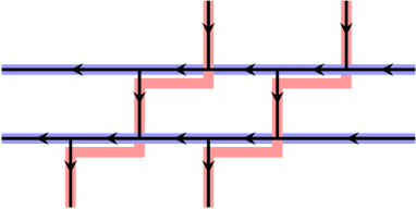
Figure 1: The modified network matrix model as a weave with extra tensor factors shown in blue (warp threads) and red (weft threads).

Summarizing, the anomaly in the $RTT$ relations can be cancelled at the expense of adding extra factors, which do not transform under the DIM algebra, to each Fock representation.

Appendix D: The $4d$ limit.

To understand the relation between network matrix models and familiar objects in CFT, we discuss in this Appendix the “$4d$ limit”: $q=e^{\hbar}\to 1$, $t=q^{\beta}$, $\beta$ fixed. Algebraically, it is described by the affine Yangian, [48]–[53]. In this limit, the intertwiners should turn into the screened vertex operators of the ordinary Virasoro or $\mathcal{W}_{m}$-algebra. We demonstrate here how this happens in detail.

In the $4d$ limit, the $q$-deformation of the free field disappears and one has

$$\left[a_{n},a_{m}\right]=\frac{n}{\beta}\delta_{m+n,0}$$ (86)

The DIM currents $\eta(z)$ and $\xi(z)$ (for fixed $z$) turn into exponentials of the ordinary Heisenberg currents:

$$\eta(z)\to:e^{\hbar\beta z\partial_{z}\phi(z)}:$$ (87)

$$\xi(z)\to:e^{-\hbar\beta z\partial_{z}\phi(z)}:$$ (88)

To get a nontrivial result for the vertices $\Psi_{\lambda}$ and $\Psi^{*}_{\lambda}$, one has to assume that the rows $\lambda_{i}$ of the Young diagram become longer and longer in the limit of $\hbar\to 0$, so that $\hbar\lambda_{i}$ is finite. It is also important that the number of rows $l(\lambda)$ remains finite. Then, the products over rows in Eqs. (51), (52) become exponentials of integrals:

$$:\prod_{(i,j)\in\lambda}\eta(zq^{j-1}t^{1-i}):\to:\prod_{i=1}^{l(\lambda)}\exp\left(\beta\int_{1}^{pe^{\hbar\lambda_{i}}}z\partial_{z}\phi(zw)\frac{dw}{w}\right):=:\prod_{i=1}^{l(\lambda)}e^{\beta\phi(x_{i})-\beta\phi(z)}:$$ (89)

$$:\prod_{(i,j)\in\lambda}\xi(zq^{j-1}t^{1-i}):\to:\prod_{i=1}^{l(\lambda)}e^{-\beta\phi(x_{i})+\beta\phi(z)}:$$ (90)

where $x_{i}=ze^{\hbar\lambda_{i}}$. Thus, the essential part of the vertex is just a product of the Dotsenko-Fateev (DF) screening currents. Notice that the number of screening currents is not fixed, but can be arbitrary, depending on the height of $\lambda$. In the end, when computing the topological string partition function, or the conformal block, one should sum over $\lambda$. In the $4d$ limit, the role of this sum is twofold: it produces a multiple integral over $x_{i}$, but also gives a sum over the number of the DF screening charges. This sum is customary in the DF formalism, since one has to accommodate for any external and internal dimensions in the conformal block.

The part of the vertex independent of the Young diagram $\Psi_{\varnothing}(z)$ diverges in the $4d$ limit. More precisely, one gets:

$$\Psi_{\varnothing}(z) \to\exp\left(\frac{1}{\hbar}\int_{0}^{z}\phi(w)\frac{dw}{w}+\frac{1}{2}\phi(z)+\mathcal{O}(\hbar)\right),$$ (91)

$$\Psi_{\varnothing}^{*}(z) \to\exp\left(-\frac{1}{\hbar}\int_{0}^{z}\phi(w)\frac{dw}{w}-\left(\beta-\frac{1}{2}\right)\phi_{-}(z)-\left(\frac{3}{2}-\beta\right)\phi_{+}(z)+\mathcal{O}(\hbar)\right),$$ (92)

The origin of this divergence can be traced back to our assumption that the position of the vertex $z$ remains finite. It turns out that one has to modify this assumption to get a meaningful operator in the $4d$ limit. The only way to cancel the divergence is to combine $\Psi(z)$ and $\Psi^{*}(w)$ pairwise on each leg, and send the spectral parameters inside the pairs towards each other, e.g. $\frac{z}{w}=q^{\alpha}$ with $\alpha$ finite. Then, the divergent parts in Eqs. (91) (92) cancel each other and we are left with the following vertex operator:

$$\Psi_{\varnothing}(z)\Psi_{\varnothing}^{*}(zq^{\alpha})\to\exp\left[(1-\beta-\alpha)\phi_{-}(z)+(\beta-1-\alpha)\phi_{+}(z)\right]$$ (93)

Notice that positive and negative modes enter with slightly different coefficients in the vertex operator (93). This leads to the special form of the so-called $U(1)$ vertex operators [54]. The pairwise arrangement of the intertwiners implies that the whole network is balanced, i.e. it is composed of the blocks of intertwiners, which conserve the slopes of the lines. The simplest block of this form is the four-leg block, which will play the role of the $T$-operator in the main text.

Let us also mention that for a special choice of the spectral parameters (a la DF, which we will use henceforth) the width of the Young diagram $\lambda$ is limited. To see this consider the product of two intertwiners:

$$\parbox{99.58464pt}{\includegraphics[width=99.58464pt]{figures/Tzero-crop}}=\Psi^{\lambda}(u|z)\Psi^{*}_{\varnothing}(-uz|w)$$ (94)

featuring as the main element of the conformal blocks. For concrete calculations the two operators should be normal ordered, which gives rise to an OPE coefficient. This coefficient contains a multiplicative factor

$$\prod_{(i,j)\in\lambda}\left(1-\sqrt{\frac{q}{t}}\frac{w}{z}q^{j-1}t^{1-i}\right)$$ (95)

If we set $\sqrt{\frac{q}{t}}\frac{w}{z}=t^{N}$ with positive integer $N$, the contribution of Young diagrams wider than $N$ is exactly zero because of the factor with $j=1$ and $i=N+1$ in the product. For example we can set $N=1$ and observe that there can only be either one or no screening currents around a given vertex operator. This is the reflection of the situation in the original DF setup for conformal block, where the possible number of screenings is governed by the dimensions of the (degenerate) external fields. In Eq. (94) we have set one of vertical Young diagrams empty. If we consider general pairs of diagrams $\lambda$ and $\mu$ the situation is analogous and there is a constraint on their relative widths.

Let us summarize what we obtained in this Appendix. In the $4d$ limit one is forced to consider asymptotically large partitions sitting on the vertical legs. This introduces asymmetry in the originally symmetric description of the network of intertwiners and breaks the spectral duality symmetry. The sums over vertical Young diagrams turn into multiple integrals, while horizontal lines still carry free field (Fock) representations. The original DIM intertwiners make no sense, unless considered in balanced pairs with coalescing spectral parameters. The pair of vertices turns into a prototype of the vertex operator with the product of screening currents as follows (we omit some normalization factors in front of the operators):

$$\parbox{99.58464pt}{\includegraphics[width=99.58464pt]{figures/T-crop}}\xrightarrow{q\to 1,t=q^{\beta},w=zq^{-\alpha}}:e^{(1-\beta-\alpha)\phi_{-}(z)+(\beta-1-\alpha)\phi_{+}(z)}\prod_{i=1}^{l(\mu)}e^{-\beta\phi(x_{i})+\beta\phi(z)}\prod_{i=1}^{l(\lambda)}e^{\beta\phi(x_{i})-\beta\phi(z)}:$$ (96)

Appendix E: Horizontal and vertical $R$-matrices.

In this Appendix, we give a simplified and hopefully elucidating example, in which horizontal and vertical $R$-matrices occur.

The horizontal and vertical $R$-matrices correspond to directions in the root space of the algebra, which parameterize the choice of the Borel subalgebra. Thus, the change from one $R$-matrix to another is associated with different choices of the Borel subalgebra.

Consider first the finite dimensional quantum algebra $U_{q}(\mathfrak{sl}_{n})$. The universal $R$-matrix is given by the product over positive roots (and the Cartan subalgebra):

$$\mathcal{R}=e^{\frac{1}{2}\sum_{i,j}\alpha^{-1}_{ij}\alpha_{ii}\alpha_{jj}H_{i}\otimes H_{j}}\prod_{\alpha\in\Delta_{+}}\exp_{q^{(\alpha,\alpha)}}\left((q-q^{-1})E_{\alpha}\otimes E_{-\alpha}\right)$$ (97)

where $\alpha_{ij}$ is the Cartan matrix of $A_{n-1}$ and the $q$-exponential is given by

$$\exp_{q}(x)=\sum_{n\geq 0}\frac{(1-q)^{n}}{\prod_{k=1}^{n}(1-q^{k})}x^{n}$$ (98)

This $R$-matrix belongs to the tensor product of positive and negative Borel subalgebras $U_{q}(\mathfrak{b}_{+})\otimes U_{q}(\mathfrak{b}_{-})$ and in this sense is a triangular matrix. In the fundamental representation, one gets the matrix (up to an overall constant):

$$\mathcal{R}_{\square,\square}=(\rho_{\square}\otimes\rho_{\square})\mathcal{R}=q\sum_{i=1}^{n}E_{ii}\otimes E_{ii}+\sum_{i\neq j}E_{ii}\otimes E_{jj}+(q-q^{-1})\sum_{i<j}E_{ij}\otimes E_{ji}$$ (99)

Notice the $i<j$ constraint in the last sum, which defines $\mathfrak{b}_{\pm}$.

If we change the Borel subalgebras $\mathfrak{b}_{\pm}$ that enter the definition of the universal $R$-matrix, i.e. rotate the hyperplane separating positive and negative roots, we get a different $R$-matrix:

$$\mathcal{R}^{\text{rot}}=e^{\frac{1}{2}\sum_{i,j}\alpha^{-1}_{ij}\alpha_{ii}\alpha_{jj}H_{i}\otimes H_{j}}\prod_{\alpha\in\Delta^{\text{rot}}_{+}}\exp_{q^{(\alpha,\alpha)}}\left((q-q^{-1})E_{\alpha}\otimes E_{-\alpha}\right)$$ (100)

However, this $R$-matrix is obtained from $\mathcal{R}$ by a simple transformation. One should conjugate $\mathcal{R}$ with the element of the Weyl group, which performs the rotation of the hyperplane in root space:

$$\mathcal{R}^{\text{rot}}=\mathcal{R}^{(\sigma)}=(\sigma\otimes\sigma)\mathcal{R}(\sigma^{-1}\otimes\sigma^{-1})$$ (101)

In the fundamental representation, the rotated $R$-matrix reads

$$\mathcal{R}^{\text{rot}}_{\square,\square}=(\rho_{\square}\otimes\rho_{\square})\mathcal{R}^{\text{rot}}=q\sum_{i=1}^{n}E_{ii}\otimes E_{ii}+\sum_{i\neq j}E_{ii}\otimes E_{jj}+(q-q^{-1})\sum_{i<j}E_{\sigma(i)\sigma(j)}\otimes E_{\sigma(j)\sigma(i)}$$ (102)

Obviously $\mathcal{R}^{\text{rot}}$ is equivalent to $\mathcal{R}$ in all respects, in particular, if $\mathcal{R}$ satisfies the Yang-Baxter equation, so does $\mathcal{R}^{\text{rot}}$.

In the case of quantum affine algebras, the situation is a bit more subtle. The $R$-matrix is again given by the product over positive roots belonging to the Borel subalgebra $\mathfrak{b}_{+}$ shown in Fig. 2, a), though now the product is infinite:

$$\mathcal{R}=\mathcal{K}\mathcal{R}_{>\delta}\mathcal{R}_{\sim\delta}\mathcal{R}_{<\delta}$$ (103)

where

$$\mathcal{K}=e^{\frac{1}{2}\sum_{i,j}\alpha^{-1}_{ij}\alpha_{ii}\alpha_{jj}H_{i}\otimes H_{j}}$$ (104)

$$\mathcal{R}_{>\delta}=\prod_{\alpha\in\Delta_{+}}\prod_{n\geq 0}\exp_{q^{(\alpha,\alpha)}}\left((q-q^{-1})E_{\alpha+n\delta}\otimes E_{-\alpha-n\delta}\right)$$ (105)

$$\mathcal{R}_{\sim\delta}=\exp\left((q-q^{-1})\sum_{n\geq 1}\sum_{i,j}u_{n,i,j}E_{n\delta,i}\otimes E_{-n\delta,j}\right)$$ (106)

$$\mathcal{R}_{<\delta}=\prod_{\alpha\in\Delta_{-}}\prod_{n\geq 1}\exp_{q^{(\alpha,\alpha)}}\left((q-q^{-1})E_{\alpha+n\delta}\otimes E_{-\alpha-n\delta}\right)$$ (107)

and $u_{n}$ is inverse of the matrix $(-1)^{n(1-\delta_{ij})}[na_{ij}]_{q}n^{-1}$. In the fundamental evaluation representation of $U_{q}(\widehat{\mathfrak{sl}}_{2})$, the parts of $R$-matrix up to a scalar multiple look as follows:

$$\rho_{z,\square}\otimes\rho_{w,\square}(\mathcal{K})=\left(\begin{array}[]{cccc}1&0&0&0\\ 0&q^{-1}&0&0\\ 0&0&q^{-1}&0\\ 0&0&0&1\\ \end{array}\right),\qquad\qquad\rho_{z,\square}\otimes\rho_{w,\square}(\mathcal{R}_{>\delta})=\left(\begin{array}[]{cccc}1&0&0&0\\ 0&1&\frac{q-q^{-1}}{1-\frac{z}{w}}&0\\ 0&0&1&0\\ 0&0&0&1\\ \end{array}\right)$$ (116)

$$\rho_{z,\square}\otimes\rho_{w,\square}(\mathcal{R}_{\sim\delta})=\left(\begin{array}[]{cccc}1&0&0&0\\ 0&\frac{1-q^{2}\frac{z}{w}}{1-\frac{z}{w}}&0&0\\ 0&0&\frac{1-\frac{z}{w}}{1-\frac{z}{q^{2}w}}&0\\ 0&0&0&1\\ \end{array}\right),\qquad\rho_{z,\square}\otimes\rho_{w,\square}(\mathcal{R}_{<\delta})=\left(\begin{array}[]{cccc}1&0&0&0\\ 0&1&0&0\\ 0&\frac{(q-q^{-1})\frac{z}{w}}{1-\frac{z}{w}}&1&0\\ 0&0&0&1\\ \end{array}\right)$$ (125)

Thus, the whole $R$-matrix is of the familiar form:

$$R\left(\frac{z}{w}\right)=\rho_{z,\square}\otimes\rho_{w,\square}(\mathcal{R})=\left(\begin{array}[]{cccc}1&0&0&0\\ 0&\frac{w-z}{qw-q^{-1}z}&\frac{(q-q^{-1})w}{qw-q^{-1}z}&0\\ 0&\frac{(q-q^{-1})z}{qw-q^{-1}z}&\frac{w-z}{qw-q^{-1}z}&0\\ 0&0&0&1\\ \end{array}\right)$$ (126)

Of course, the form of the $R$-matrix again depends on the choice of the Borel subalgebra $\mathfrak{b}_{+}$. First of all, there is an infinite set of $R$-matrices $\mathcal{R}^{\mathrm{rot}}$ obtained from a given one by action of the affine Weyl group. They are given by expressions similar to Eq. (101).

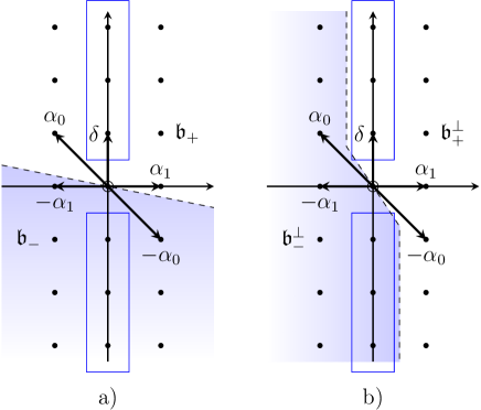
Figure 2: a) The root system of $U_{q}(\widehat{\mathfrak{sl}}_{2})$ with the standard choice of positive roots $\alpha_{1}$ and $\alpha_{0}=\delta-\alpha_{1}$ and the corresponding “vertical” Borel subalgebras $\mathfrak{b}_{-}$ (shaded) and $\mathfrak{b}_{+}$. b) The “horizontal” Borel subalgebras $\mathfrak{b}^{\perp}_{\pm}$. The modes of the Cartan current $H(z)$ are shown in blue boxes.

Most importantly, there is one distinct choice of the Borel subalgebra denoted by $\mathfrak{b}^{\perp}$ which cannot be obtained from the standard one by the action of the Weyl group: one can choose the subalgebra “in the perpendicular direction” (see Fig. 2, b)). This choice is natural in Drinfeld’s “new realization” of quantum affine algebras and can be thought of as a limiting case, when one acts with the $T_{\theta}^{n}$ generator of the affine Weyl group with a sufficiently high power $n$. Let us compute this “perpendicular” $R$-matrix in the evaluation representation. What we need is just a minor variation of the Khoroshkin-Tolstoy expression (103). The $R$-matrix is given by the product

$$\mathcal{R}^{\perp}=\mathcal{K}\mathcal{R}_{>\delta}^{\prime}\mathcal{R}_{\sim\delta}$$ (127)

Notice that there is no usual $R_{<\delta}$ term in the product and instead, the $R_{>\delta}$ term is modified:

$$\mathcal{R}^{\prime}_{>\delta}=\prod_{\alpha\in\Delta_{+}}\prod_{n\in\mathbb{Z}}\exp_{q^{(\alpha,\alpha)}}\left((q-q^{-1})E_{\alpha+n\delta}\otimes E_{-\alpha-n\delta}\right)$$ (128)

Performing the calculation, we find

$$\rho_{z,\square}\otimes\rho_{w,\square}(\mathcal{R}_{>\delta}^{\prime})=\left(\begin{array}[]{cccc}1&0&0&0\\ 0&1&(q-q^{-1})\delta\left(\frac{z}{w}\right)&0\\ 0&0&1&0\\ 0&0&0&1\\ \end{array}\right)$$ (133)

where $\delta(x)=\sum_{n\in\mathbb{Z}}x^{n}$. Multiplying this modified matrix with $\mathcal{R}_{\sim\delta}$, one finds that the $\delta$-function term is annihilated since $(1-x)\delta(x)=0$ and the perpendicular $R$-matrix is diagonal:

$$R^{\perp}\left(\frac{z}{w}\right)=\rho_{z,\square}\otimes\rho_{w,\square}(\mathcal{R}^{\perp})=\rho_{z,\square}\otimes\rho_{w,\square}(\mathcal{K}\mathcal{R}_{\sim\delta})=\left(\begin{array}[]{cccc}1&0&0&0\\ 0&\frac{q^{-1}w-qz}{w-z}&0&0\\ 0&0&\frac{w-z}{qw-q^{-1}z}&0\\ 0&0&0&1\\ \end{array}\right)$$ (134)

$\mathcal{R}^{\perp}$ trivially satisfies the Yang-Baxter equation and the relation $\mathcal{R^{\perp}}(x^{-1})=P(\mathcal{R}^{\perp}(x))^{-1}P$. The $R$-matrix (134) differs from the familiar one (126) by a twist, which is nothing, but the product over a “quarter” of the roots [31, 55].

There are several lessons to learn from this example. $\mathcal{R}$ and $\mathcal{R}^{\perp}$ are very similar to the $R$-matrices of the DIM algebra taken in the basis of Macdonald and generalized Macdonald polynomials respectively. The natural basis of weight vectors $\left|z,\pm\frac{1}{2}\right\rangle$ in the evaluation representation is a counterpart of the generalized Macdonald basis. Indeed, generalized Macdonald polynomials are eigenvalues of $\Delta(x^{+}_{0})$, which can be thought of as a Cartan generator of DIM. Similarly, we have

$$\rho_{z,\square}\otimes\rho_{w,\square}(\Delta^{D}(H_{1}))\left|z,\pm\frac{1}{2}\right\rangle\otimes\left|w,\pm\frac{1}{2}\right\rangle=(\pm z\pm w)\left|z,\pm\frac{1}{2}\right\rangle\otimes\left|w,\pm\frac{1}{2}\right\rangle$$ (135)

where $H_{1}$ is the first mode of the Drinfeld current $H(z)$, which is the Cartan generator. Notice that here $\Delta^{D}$ is not the standard coproduct $\Delta$, which would have led to the standard $R$-matrix (126), but the second coproduct [31, 56], which is also known as the Drinfeld coproduct.

The evaluation representation can be thus interpreted as “vertical”, since we can diagonalize the “vertical” Cartan generators $H(z)$ in it. What are the “horizontal” representations? It seems natural that those are the highest weight representations of the affine algebra. It is technically difficult to derive the $R$-matrix in these representations. However, we hope that if computed, this $R$-matrix, among other things, can be used to obtain new and interesting knot invariants.

References

• [1] J. Ding, K. Iohara, Lett. Math. Phys. 41 (1997) 181–193, q-alg/9608002
• [2] K. Miki, J. Math. Phys. 48 (2007) 123520
• [3] B. Feigin and A. Tsymbaliuk, Kyoto J. Math. 51 (2011) 831-854, arXiv:0904.1679
B. Feigin, E. Feigin, M. Jimbo, T. Miwa and E. Mukhin, Kyoto J. Math. 51 (2011) 337-364, arXiv:1002.3100
B. Feigin, K. Hashizume, A. Hoshino, J. Shiraishi and S. Yanagida, J. Math. Phys. 50 (2009) 095215, arXiv:0904.2291
• [4] B. Feigin, A. Hoshino, J. Shibahara, J. Shiraishi and S. Yanagida, arXiv:1002.2485
• [5] B. Feigin, E. Feigin, M. Jimbo, T. Miwa and E. Mukhin, Kyoto J. Math. 51 (2011) 365-392, arXiv:1002.3113
• [6] H. Awata, B. Feigin, A. Hoshino, M. Kanai, J. Shiraishi and S. Yanagida, RIMS kōkyūroku 1765 (2011) 12 – 32; arXiv:1106.4088
• [7] B. Feigin, M. Jimbo, T. Miwa and E. Mukhin, Kyoto J. Math. 52, no. 3 (2012), 621-659, arXiv:1110.5310
• [8] H. Awata, B. Feigin and J. Shiraishi, arXiv:1112.6074
• [9] B. Feigin, M. Jimbo, T. Miwa and E. Mukhin, arXiv:1502.07194
• [10] B. Feigin, M. Jimbo, T. Miwa and E. Mukhin, arXiv:1603.02765
• [11] H. Awata, H. Kanno, A. Mironov, A. Morozov, A. Morozov, Y. Ohkubo and Y. Zenkevich, JHEP, 10 (2016) 047, arXiv:1608.05351
• [12] A. Morozov and Y. Zenkevich, JHEP 1602 (2016) 098, arXiv:1510.01896
• [13] T. Kimura and V. Pestun, arXiv:1512.08533
J. E. Bourgine, M. Fukuda, Y. Matsuo, H. Zhang and R. D. Zhu, arXiv:1606.08020
• [14] A. Mironov, A. Morozov, Y. Zenkevich, Phys. Lett. B756 (2016) 208-211, arXiv:1512.06701; JHEP, 05 (2016) 121, arXiv:1603.00304; Phys.Lett. B762 (2016) 196-208, arXiv:1603.05467
• [15] H. Awata, H. Kanno, T. Matsumoto, A. Mironov, A. Morozov, An. Morozov, Y. Ohkubo and Y. Zenkevich, JHEP, 07 (2016) 103, arXiv:1604.08366
• [16] N. Seiberg and E. Witten, Nucl. Phys. B426 (1994) 19-52, hep-th/9407087; Nucl. Phys. B431 (1994) 484-550, hep-th/9408099
• [17] A.Gorsky, I.Krichever, A.Marshakov, A.Mironov, A.Morozov, Phys.Lett. B355 (1995) 466, hep-th/9505035
R. Donagi and E. Witten, Nucl. Phys. B460 (1996) 299-334, hep-th/9510101
E. Martinec, Phys. Lett. B367 (1996) 91-96, hep-th/9510204
E. Martinec and N. Warner, Nucl. Phys. 459 (1996) 97, hep-th/9511052
• [18] N. Nekrasov, Adv. Theor. Math. Phys. 7 (2004) 831-864, hep-th/0206161
R. Flume and R. Pogossian, Int. J. Mod. Phys. A18 (2003) 2541, hep-th/0208176
N. Nekrasov and A. Okounkov, hep-th/0306238
• [19] A. Iqbal, hep-th/0207114
M. Aganagic, A. Klemm, M. Marino and C. Vafa, Commun. Math. Phys. 254 (2005) 425 hep-th/0305132
A. Okounkov, N. Reshetikhin and C. Vafa, hep-th/0309208
T. Eguchi and H. Kanno, JHEP 0312 (2003) 006, hep-th/0310235
A. Iqbal, N. Nekrasov, A. Okounkov and C. Vafa, JHEP 0804 (2008) 011, hep-th/0312022
H. Awata and H. Kanno, JHEP 0505 (2005) 039, hep-th/0502061
• [20] A. Iqbal, C. Kozcaz and C. Vafa, JHEP 0910 (2009) 069, hep-th/0701156
• [21] H. Awata and H. Kanno, Int. J. Mod. Phys. A 24, 2253 (2009), arXiv:0805.0191
• [22] L. Alday, D. Gaiotto and Y. Tachikawa, Lett. Math. Phys. 91 (2010) 167–197, arXiv:0906.3219
N. Wyllard, JHEP 0911 (2009) 002, arXiv:0907.2189
A. Mironov and A. Morozov, Nucl. Phys. B825 (2009) 1–37, arXiv:0908.2569
• [23] N. Nekrasov and S. Shatashvili, arXiv:0908.4052
A. Mironov and A. Morozov, JHEP 04 (2010) 040, arXiv:0910.5670; J. Phys. A43 (2010) 195401, arXiv:0911.2396
A. Marshakov, A. Mironov and A. Morozov, J. Geom. Phys. 61 (2011) 1203-1222, arXiv:1011.4491
• [24] H. Awata and Y. Yamada, JHEP 1001 (2010) 125, arXiv:0910.4431; Prog. Theor. Phys.  124 (2010) 227, arXiv:1004.5122
S. Yanagida, arXiv:1005.0216
A. Mironov, A. Morozov, S. Shakirov and A. Smirnov, Nucl. Phys. B855 (2012) 128, arXiv:1105.0948
F. Nieri, S. Pasquetti and F. Passerini, arXiv:1303.2626
F. Nieri, S. Pasquetti, F. Passerini and A. Torrielli, arXiv:1312.1294
M.-C. Tan, JHEP 12 (2013) 031, arXiv:1309.4775; arXiv:1607.08330
H. Itoyama, T.Oota and R. Yoshioka, arXiv:1408.4216, arXiv:1602.01209
A. Nedelin and M. Zabzine, arXiv:1511.03471
R. Yoshioka, arXiv:1512.01084
Y. Ohkubo, H. Awata and H. Fujino, arXiv:1512.08016
S. Pasquetti, arXiv:1608.02968
• [25] V. Drinfeld, Doklady Akad. Nauk SSSR 283 (1985) 1060
M. Jimbo, Lett. Math. Phys. 10 (1985) 63-69; ibid. 11 (1986) 247-252; Commun. Math. Phys. 102 (1986) 537-547
• [26] N.Yu. Reshetikhin, L.A. Takhtadjan and L.D. Faddeev, Algebra and Analysis, 1 (1989) 178-206
• [27] V. Drinfeld, Quantum groups, in: Proceedings of the International Congress of Mathematicians, Berkeley, (1986), Ed. by A. M. Gleason (AMS, Providence, 1987), pp. 798-820; Algebra Anal. 1 (1989) 30-46
• [28] C. Fronsdal and A. Galindo, The Universal T-Matrix, preprint UCLA/93/TEP/2, Jan. 1993, 16p.
A. Morozov, L. Vinet, hepth/9409093
A. Mironov, Theor.Math.Phys. 114 (1998) 127, q-alg/9711006; hep-th/9409190
• [29] See a review and references, e.g., in:
M. Jimbo, Topics from Representations of $U_{q}(g)$. An Introductory Guide to Physicists, Nankai Lectures on Mathematical Physics, 1992: World Scientific, Singapore, pp. 1-61
• [30] H. Boos, F. Göhmann, A. Klümper, Kh. Nirov, A. Razumov, J.Phys. A: Math.Theor. 43 (2010) 415208, arXiv:1004.5342
• [31] V.G. Drinfeld, Soviet Math. Doklady, 36 (1988) 212-216
• [32] E. Mukhin, V. Tarasov and A. Varchenko, math/0510364; Adv. Math. 218 (2008) 216-265, math/0605172
A. Mironov, A. Morozov, Y. Zenkevich and A. Zotov, JETP Lett. 97 (2013) 45, arXiv:1204.0913
A. Mironov, A. Morozov, B. Runov, Y. Zenkevich and A. Zotov, Lett. Math. Phys. 103 (2013) 299, arXiv:1206.6349; JHEP 1312 (2013) 034, arXiv:1307.1502
L. Bao, E. Pomoni, M. Taki and F. Yagi, JHEP 1204 (2012) 105, arXiv:1112.5228
• [33] A. Okounkov and A. Smirnov, arXiv:1602.09007
• [34] A. Morozov and A. Smirnov, Lett.Math.Phys. 104 (2014) 585, arXiv:1307.2576
• [35] S. Mironov, A. Morozov and Y. Zenkevich, JETP Lett.  99 (2014) 109, arXiv:1312.5732
• [36] Y. Ohkubo, arXiv:1404.5401
• [37] Y. Zenkevich, JHEP 1505 (2015) 131, arXiv:1412.8592
• [38] Y. Kononov and A. Morozov, Eur.Phys.J. C76 (2016) 424 arXiv:1607.00615
Y. Zenkevich, to appear
• [39] A. V. Litvinov, JHEP 1311 (2013) 155, arXiv:1307.8094
M. N. Alfimov and A. V. Litvinov, JHEP 1502 (2015) 150, arXiv:1411.3313
G. Bonelli, A. Sciarappa, A. Tanzini and P. Vasko, JHEP 7 (2014) 141, arXiv:1403.6454; arXiv:1505.07116
P. Koroteev and A. Sciarappa, arXiv:1510.00972; arXiv:1601.08238
• [40] E. Guadagnini, M. Martellini and M. Mintchev, In Clausthal 1989, Proceedings, Quantum groups, 307-317; Phys.Lett. B235 (1990) 275;
N.Yu. Reshetikhin and V.G. Turaev, Comm. Math. Phys. 127 (1990) 1-26
• [41] A. Mironov, A. Morozov and An. Morozov, in: Strings, Gauge Fields, and the Geometry Behind: The Legacy of Maximilian Kreuzer, edited by A. Rebhan, L. Katzarkov, J. Knapp, R. Rashkov, E. Scheidegger (World Scietific Publishins Co.Pte.Ltd. 2013) pp.101-118, arXiv:1112.5754; JHEP 03 (2012) 034, arXiv:1112.2654
A. Anokhina, A. Mironov, A. Morozov and An. Morozov, Nucl.Phys. B868 (2013) 271-313, arXiv:1207.0279
• [42] K. Murasugi, Knot Theory and Its Applications, Birkhauser, Boston MA, 1996
• [43] E. Witten, arXiv:1611.00592
• [44] K. Costello, arXiv:1303.2632; arXiv:1308.0370
• [45] M. Aganagic and A. Okounkov, arXiv:1604.00423
• [46] M. Wakimoto, Commun. Math. Phys. 104 (1986) 605-609
A. Gerasimov, A. Marshakov, A. Morozov, M. Olshanetsky, S. Shatashvili, Int.J.Mod.Phys. A5 (1990) 2495
B. Feigin and E. Frenkel Phys. Lett. B246 (1990) 75-81
• [47] M. Taki, JHEP 0803 (2008) 048, arXiv:0710.1776
• [48] N. Guay, Adv. Math. 211 (2007) 436-484
N. Arbesfeld and O. Schiffmann, arXiv:1209.0429
A. Tsymbaliuk, arXiv:1404.5240
M. Bernshtein and A. Tsymbaliuk, arXiv:1512.09109
T. Prochazka, arXiv:1512.07178
• [49] O. Schiffmann and E. Vasserot, Compositio Mathematica 147 (2011) 188-234, arXiv:0802.4001; Duke Mathematical Journal 162 (2013) 279–366, arXiv:0905.2555; arXiv:1202.2756
• [50] D. Maulik and A. Okounkov, arXiv:1211.1287
• [51] A. Smirnov, arXiv:1302.0799, arXiv:1404.5304
• [52] R.-D. Zhu and Y. Matsuo, Prog. Theor. Exp. Phys. (2015) 093A01, arXiv:1504.04150
M. Fukuda, S. Nakamura, Y. Matsuo and R.-D. Zhu, arXiv:1509.01000
• [53] J.-E. Bourgine, Y. Matsuo and H. Zhang, arXiv:1512.02492
• [54] E. Carlsson and A. Okounkov, arXiv:0801.2565
• [55] B. Enriquez, S. Khoroshkin and S. Pakuliak, Commun.Math.Phys. 276 (2007) 691-725, math/0610398
• [56] B. Feigin, M. Jimbo, T. Miwa and E. Mukhin, arXiv:1609.05724