Derivation of human chromatic discrimination ability from an information-theoretical notion of distance in color space

Abstract

The accuracy with which humans can detect small chromatic differences varies throughout color space. For example, we are far more precise when discriminating two similar orange stimuli than two similar green stimuli. In order for two colors to be perceived as different, the neurons representing chromatic information must respond differently, and the difference must be larger than the trial-to-trial variability of the response to each separate color. Photoreceptors constitute the first stage in the processing of color information; many more stages are required before humans can consciously report whether two stimuli are perceived as chromatically distinguishable or not. Therefore, although photoreceptor absorption curves are expected to influence the accuracy of conscious discriminability, there is no reason to believe that they should suffice to explain it. Here we develop information-theoretical tools based on the Fisher metric that demonstrate that photoreceptor absorption properties explain $\approx~{}87$% of the variance of human color discrimination ability, as tested by previous behavioral experiments. In the context of this theory, the bottleneck in chromatic information processing is determined by photoreceptor absorption characteristics. Subsequent encoding stages modify only marginally the chromatic discriminability at the photoreceptor level.

1 Introduction

Perception is the subjective experience that results from the entire brain, not just photoreceptors. Color discrimination tasks rely on the ability to detect small differences in the activity of higher brain areas when two stimuli of similar chromatic composition are presented. Human color discrimination ability has been measured by several authors with behavioral experiments first performed by Wright and Pitt (1934). In these studies, a bipartite field was presented to a human subject. One half of the field, here called the reference field, was illuminated by a monochromatic beam, constructed by filtering a broad-band light source. The second half, the test field, was also monochromatic, and its wavelength was controlled by the observer. Initially, the two beams had the same wavelength and luminosity. The observer was instructed to displace the wavelength of the test field, until the first noticeable difference in hue was perceived. At this point, the difference $\Delta\lambda$ between the reference and test wavelengths was calculated. This difference constitutes the discrimination error, that is, the interval in wavelengths below which the two colors cannot be perceptually discriminated. The discrimination error was reported to be a W-shaped function of wavelength, as displayed in Fig.1A (Wright and Pitt 1934; Pokorny and Smith, 1970).

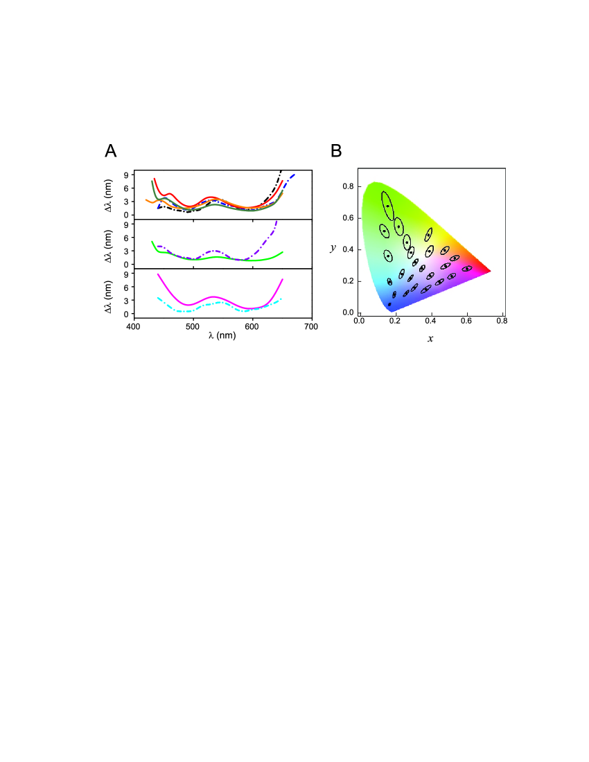
Figure 1: Previous experimental results of human color discrimination ability. A: Discrimination error $\Delta\lambda$ as a function of the wavelength $\lambda$ of the reference beam, measured in behavioral experiments for 9 different subjects. All subjects exhibit a local maximum at $\lambda\approx 550$ nm. Subjects are separated in 3 groups, depending on the shape of the curve at $\lambda\approx 450$ nm. Top: Subjects exhibiting a local maximum. Middle: Subjects exhibiting a shoulder. Bottom: Subjects with monotonically decreasing errors. Data from Wright and Pitt (1934) and Pokorny and Smith (1970). B: MacAdam ellipses (MacAdam 1942) in the CIE 1931 $xy$ chromaticity diagram, reporting the region in color space that is confounded with the center. As customary, each ellipse is enlarged 10 times in each dimension for better visualization.

Different curves correspond to different subjects. For all subjects, discrimination errors were large towards the two borders of the visible spectrum, and at around 550 nm, roughly at the center of the visible spectrum where luminosity sensitivity is maximal (Sharpe et al. 2005). At short wavelengths, the data show some variability across subjects. We have therefore separated the 9 curves into 3 groups (displayed in different panels), depending on whether the discrimination error exhibited an additional maximum at approximately 450 nm (top panel), only a shoulder (middle panel), or a monotonic behavior (bottom panel).

In 1942, David MacAdam (1942) broadened these discriminability experiments testing the ability to distinguish any two neighboring points in the entire color space, not just the subset of light beams composed of a single wavelength. The concept of color, in fact, cannot be restricted to wavelength. Blends of wavelengths produce a new chromatic sensation that emerges exclusively from the mixture, the hue of which differs from the hues of the individual components. In order to test human chromatic discrimination ability in the entire color space, MacAdam measured ellipses in the CIE 1931 $xy$ chromaticity diagram, here shown in Fig. 1B. Points in this space represent hue and saturation, and are independent of the total luminosity. Each ellipse in the diagram indicates the area in color space (multiplied by 10, for better visualization) inside which two different stimuli cannot be discriminated.

In this study, we test how much of the results in Fig. 1 can be explained from a given noise model. The basic assumption is that two colors can be discriminated when the trial-to-trial variability of their neural representations is smaller than the difference of the corresponding means. The discriminability $d^{\prime}$ of two colors is proportional to the square root of the Fisher information (Seung and Sompolinsky, 1993). The Fisher information, in turn, introduces a notion of distance in color space. Hence, our working hypothesis is that two colors become distinguishable when the Fisher distance between them is larger than a given fixed minimum: the detection threshold.

Fisher Information has been successfully used as a tool to disclose computational strategies in the nervous system for decades (see for example Abbot and Dayan 1999, Dayan and Abbot 2001, Brunel and Nadal 1998) and continues to be widely employed (Ganguli and Simoncelli 2014, Wei and Stocker 2015). Within the Fisher framework, two previous studies (Clark and Skaff 2009; Zhaoping et al. 2011) have derived the discrimination accuracy expected by an ideal observer that only has access to the number of photons absorbed by the three types of cones. Both studies were restricted to light beams composed of a single wavelength, and succeeded in explaining the W-shaped function of Fig. 1A. Our starting point is the work of Zhaoping et al. (2011). We first express the main result of their work in terms of an analytical expression for the discrimination error. We use the theory to speculate how putative tetrachromat subjects perceive the chromatic space. In the case of trichromats, we interpret the subject-to-subject variations in Fig. 1A as resulting from the reported variability in the composition of the human retina. More importantly, we derive new information-theoretical tools that expand the analysis to the entire chromatic space, beyond monochromatic light beams. By considering mixtures of wavelengths, we provide a theoretical framework to also explain Fig. 1B. By focusing our attention on the curved border of the chromatic space of Fig. 1B, we also recover the previous result with monochromatic light beams of Fig. 1A.

Our analysis concludes that 87% of the variance of MacAdam’s data can be explained by properties of photoreceptors alone. Discrimination errors reported in behavioral experiments are the result of the entire chain of hue-dependent computations intervening in chromatic perception. Therefore, the agreement between experiment and theory implies that the bottleneck in chromatic information processing seems to be mainly determined by photoreceptor activity. Subsequent encoding stages either operate optimally or, if they do not, loose information in a color-independent manner.

2 Representations of color space

Color is the subjective sensation that results when a light beam of spectrum $I(\lambda)$ impinges the eye. The set of all possible spectra has infinite dimension, since for a continuum of wavelengths $\lambda$ the intensity $I(\lambda)$ can vary arbitrarily. The human visual system, however, is insensitive to most of these dimensions. Classical behavioral color-matching experiments demonstrated that for most observers, three monochromatic light sources, conveniently mixed, suffice to reproduce all visible colors. Therefore, the human visual system projects the space of all possible spectra on a 3-dimensional subspace. All spectra sharing the same projection are metamers, that is, are perceived as indistinguishable. To represent colors as 3-dimensional vectors, here we use the coordinates $(X,Y,Z)$ defined in the CIE 1931 (Appendix A1). When two color vectors $(X_{1},Y_{1},Z_{1})$ and $(X_{2},Y_{2},Z_{2})$ only differ in their length (they are proportional to one another), they share the same hue and saturation, and can only be distinguished by their luminosity. In some applications, it is desirable to discard the luminosity dimension, and only retain the two remaining features. The CIE 1931 meeting also established a convention to carry out this reduction, by transforming the coordinates $(X,Y,Z)$ into a new set of coordinates $(x,y,Y)$ defined by

$$\begin{array}[]{lll}x=\frac{X}{X+Y+Z},&y=\frac{Y}{X+Y+Z},&Y=Y.\end{array}$$ (1)

The components $x$ and $y$ do not vary if $X,Y$ and $Z$ are all multiplied by the same factor, so $x$ and $y$ no longer contain the luminosity dimension. The variable $Y$ is associated with the sensation of brightness, since for monochromatic spectra, the wavelength dependence of $Y$ closely resembles the apparent luminosity curve (Sharpe et al, 2005). MacAdam’s experiment was reported in CIE $xy$ chromatic space (Fig. 1).

3 Statistics of the photon shower

For monochromatic light sources of mean intensity $I$ and wavelength $\lambda$, the probability $P(\overrightarrow{K}|\lambda)$ that $\overrightarrow{K}=(K_{S},K_{M},K_{L})$ photons are absorbed by $S,M$ and $L$ cones is (Appendix A2)

$$P[\overrightarrow{K}|\lambda]=\prod_{i\in\{S,M,L\}}{\rm Poisson}[K_{i}|Iq_{i}(\lambda)],$$ (2)

where ${\rm Poisson}(x|y)$ represents a Poisson distribution of the random variable $x$ with mean $y$, $q_{i}(\lambda)=\beta_{i}h_{i}(\lambda)$, the functions $h_{i}(\lambda)$ are the spectral sensitivities of cones of type $i$ illustrated in Fig. 2,

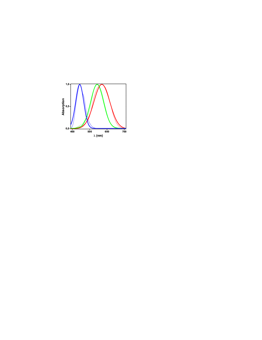
Figure 2: Quantal cone fundamentals for $S$ (blue), $M$ (green) and $L$ (red) cones, and their analytic approximations. Thin lines: Data from Stockman and Brainard (2009). Thick lines: fitted equation $h_{i}(\lambda)=\exp[-(\lambda-\lambda_{i})^{2}/\sigma_{i}^{2}]$ with $\lambda_{S}=442.1$ nm, $\lambda_{M}=542.8$ nm, $\lambda_{L}=568.2$ nm, $\sigma_{S}=32.96$ nm, $\sigma_{M}=52.8$ nm, and $\sigma_{L}=64.76$ nm.

and the parameters $\beta_{i}$ are the normalized cross sections associated with each fate of the photon. If $A_{0}$ is the retinal area not covered by cones,

$$\beta_{i}=\frac{W_{i}A_{i}}{A_{0}+\sum_{j\in\{S,M,L\}}W_{j}A_{j}}\ \ {\rm for}\ i\in\{S,M,L\},\ \ \ \beta_{0}=\frac{A_{0}}{A_{0}+\sum_{j\in\{S,M,L\}}W_{j}A_{j}}$$ (3)

where $W_{i}$ is the number of photoreceptors of type $i$, and $A_{i}$ is the cross section of each cone.

The light source is now assumed to have an arbitrary spectrum $I(\lambda)$. Defining the coefficients

$$\alpha_{i}=\int I(\lambda)\ q_{i}(\lambda)\ {\rm d}\lambda,\ \ \ {\rm for}\ i\in\{S,M,L\},$$ (4)

we show in Appendix A2 that

$$P[\overrightarrow{K}|I(\lambda)]=\prod_{\ell\in\{S,M,L\}}\ {\rm Poisson}(K_{i}|\alpha_{i}).$$ (5)

As expected, Eq. 5 reduces to Eq. 2 when the spectrum $I(\lambda)$ represents a monochromatic source, that is, for $I(\lambda)=I\ \delta(\lambda-\lambda_{0})$.

4 The geometry of color space

In simple discrimination experiments, the perceptual properties of color are contained in the number of photons absorbed by $S$, $M$ and $L$ cones. The probability that $S$, $M$ or $L$ cones absorb $K_{S}$, $K_{M}$ and $K_{L}$ photons, respectively, depends on the properties of the impinging light beam. Here we consider two types of experiments: Monochromatic beams of fixed intensity and varying wavelength, and light sources composed of arbitrary spectra. In the first case the light beam is characterized by the wavelength $\lambda$, and in the second case, by the vector $(\alpha_{S},\alpha_{M},\alpha_{L})$. Distances in color space—in $\lambda$ space, or in $(\alpha_{S},\alpha_{M},\alpha_{L})$ space—are defined by the effect on the number of absorbed photons $\overrightarrow{K}$ caused by changes in the composition of the light source. The Fisher information $J$ is a metric tensor (Appendix A3) that defines scalar products and distances in color space. In the monochromatic case, since $\lambda$ is a 1-dimensional parameter, the Fisher tensor reduces to the scalar

$$J(\lambda)=-\left\langle\frac{\partial^{2}}{\partial\lambda^{2}}\ln P\left(\overrightarrow{K}|\lambda\right)\right\rangle_{P\left(\overrightarrow{K}|\lambda\right)},$$ (6)

where the angular brackets indicate average with respect to the indicated distribution. In the case of arbitrary mixtures of wavelengths, $J$ is a tensor represented by a $3\times 3$ matrix. In coordinates $\overrightarrow{\alpha}=(\alpha_{S},\alpha_{M},\alpha_{L})$ its components are

$$J_{ij}=-\left\langle\frac{\partial^{2}}{\partial\alpha_{i}\partial\alpha_{j}}\ln P\left(\overrightarrow{K}|\overrightarrow{\alpha}\right)\right\rangle_{P\left(\overrightarrow{K}|\overrightarrow{\alpha}\right)}.$$ (7)

The Cramér-Rao bound relates the Fisher tensor to the accuracy with which the random vector $\overrightarrow{K}$ can be used to estimate the coordinates of color space. Formally, this means that the mean quadratic error of any unbiased estimator of the wavelength $\lambda$ or the coordinates $(\alpha_{S},\alpha_{M},\alpha_{L})$ from the absorbed photons $\overrightarrow{K}$ is bounded from below (Appendix A3).

Metric tensors define scalar products. In Fig. 3A

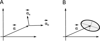
Figure 3: Scalar products in the space of parameters. A: The Fisher information metric tensor defines scalar products between two vectors $\overrightarrow{\alpha}^{a}$ and $\overrightarrow{\alpha}^{b}$ with common origin at location $\overrightarrow{\alpha}$ (Eq. 8). B: The set of all vectors at a constant distance from location $\overrightarrow{\alpha}$ defines an ellipsoid, whose principal axes are displayed with dashed lines.

we see how such products operate in the parameter space. The scalar product between two vectors $\overrightarrow{\alpha}^{a}$ and $\overrightarrow{\alpha}^{b}$ is

$$\langle\overrightarrow{\alpha}^{a},\overrightarrow{\alpha}^{b}\rangle=(\overrightarrow{\alpha}^{a})^{T}\ J(\overrightarrow{\alpha})\ \overrightarrow{\alpha}^{b},$$ (8)

where the supra-script $T$ represents vector transposition. The length of a vector $\overrightarrow{\alpha}^{a}$ originated at $\overrightarrow{\alpha}$ is then

$$\left|\overrightarrow{\alpha}^{a}\right|=\sqrt{\langle\overrightarrow{\alpha}^{a},\overrightarrow{\alpha}^{a}\rangle}=\sqrt{(\overrightarrow{\alpha}^{a})^{T}\ J(\overrightarrow{\alpha})\ \overrightarrow{\alpha}^{a}}.$$ (9)

Equation 9 implies that the set of vectors at a constant distance of a certain $\overrightarrow{\alpha}$ is a conic. Since the eigenvalues of the Fisher tensor are always non-negative, the conic is an ellipsoid (Fig. 3B). The directions of the principal axes of the ellipse are the eigenvectors of $J(\overrightarrow{\alpha})$, which are also the eigenvectors of $[J(\overrightarrow{\alpha})]^{-1}$. The lengths of those axes are proportional to the inverse of the square root of the corresponding eigenvalues of $J(\overrightarrow{\alpha})$, or equivalently, to the square root of the eigenvalues of $[J(\overrightarrow{\alpha})]^{-1}$. Since $J$ depends on $\overrightarrow{\alpha}$, the size, excentricity and orientation of the ellipse may well vary from point to point.

In Fig. 1B, the CIE 1931 $xy$ chromatic space has coordinates $(x,y)$. Each ellipse measured by MacAdam represents the set of points in color space where the first detectable chromatic difference with the point at the center is perceived. The ellipses represent the points at distance $\delta$ from the center, where $\delta$ is the detection threshold. In this paper we aim at evaluating up to which point the ellipses measured by MacAdam can be derived from the properties of photoreceptors.

We now consider two different coordinate systems $\overrightarrow{\alpha}$ and $\overrightarrow{\alpha}^{\prime}$ to represent colors. Let $\overrightarrow{F}$ be the vectorial function involved in the mapping between them:

$$\overrightarrow{\alpha}^{\prime}=\overrightarrow{F}(\overrightarrow{\alpha}).$$ (10)

The matrix representation of the Fisher tensor transforms as (Appendix A3)

$$J(\overrightarrow{\alpha})=C^{T}\ J^{\prime}(\overrightarrow{\alpha}^{\prime})\ C,$$ (11)

with $C$ defined by the Jacobian matrix

$$C=\left(\begin{array}[]{ccc}\frac{\partial F_{1}}{\partial\alpha_{1}}&\dots&\frac{\partial F_{1}}{\partial\alpha_{d}}\\ \vdots&&\vdots\\ \frac{\partial F_{d}}{\partial\alpha_{1}}&\dots&\frac{\partial F_{d}}{\partial\alpha_{d}}\end{array}\right).$$ (12)

5 Discrimination of two similar wavelengths

For a monochromatic light beam of fixed intensity $I$, Eq. 2 establishes a probabilistic mapping between each wavelength $\lambda$ and the vector $\overrightarrow{K}$. The components $K_{S},K_{M}$ and $K_{L}$ are converted to electrical signals by photoreceptors, and then processed by the rest of the brain. From the information-theoretic point of view, the data processing inequality (Amari and Nagaoka, 2000) ensures that the chromatic information encoded in later processing stages cannot exceed the amount of chromatic information contained in $\overrightarrow{K}$. A conscious subject, therefore, cannot have better discrimination ability than that of an optimal estimator inferring the wavelength $\lambda$ from photoreceptor activity, that is, from $\overrightarrow{K}$. The optimal estimator is usually referred to as the ideal observer. The Cramér-Rao bound in this case reduces to its 1-dimensional form (Cramér, 1946), $\Delta\lambda\geq 1/\sqrt{J(\lambda)}$, implying that the minimal error of the ideal observer is the inverse of the square root of the Fisher information $J(\lambda)$.

Throughout the paper, spectral sensitivity curves were taken from the cone fundamentals reported by Stockman and Brainard (2009). In order to work with differentiable functions, the experimental curves were approximated by functions $h_{i}(\lambda)=\exp[-(\lambda-\lambda_{i})^{2}/\sigma_{i}^{2}]$, with fitting parameters $\lambda_{i}$ and $\sigma_{i}$, coinciding with the position of the peak and the width of the data. Both the original and the fitted curves are displayed in Fig. 2 (fitted parameters in the figure caption). Using this approximation, we insert Eq. 2 in Eq. 7 and get

$$J(\lambda)=I\sum_{i\in\{S,M,L\}}\frac{\left[q_{i}^{\prime}(\lambda)\right]^{2}}{q_{i}(\lambda)}\\ =4I\sum_{i\in\{S,M,L\}}\ \frac{(\lambda-\lambda_{i})^{2}}{\sigma_{i}^{4}}\ {\rm e}^{-(\lambda-\lambda_{i})^{2}/\sigma_{i}^{2}}.$$ (13)

The formal expression of Eq. 13 was derived by Dayan and Abbot (2001), and was first applied to the chromatic context by Zhaoping et al (2011). Here we provide the analytical expression at the right of Eq. 13. Note that the amount of Fisher information is proportional to the intensity of the light source, in Eq. 13 represented by the mean number of photons $I$.

In Fig. 4, we display the minimal estimation error $\Delta\lambda=1/\sqrt{J(\lambda)}$

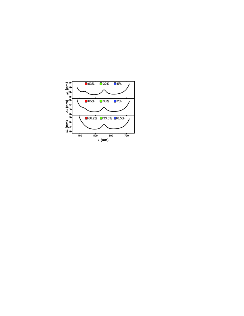
Figure 4: Minimal discrimination error $\Delta\lambda$ as a function of the reference wavelength $\lambda$, obtained from Eq. 13. Different curves correspond to different proportions of $S$ (blue), $M$ (green) and $L$ (red) cones, as indicated in the legends. For all wavelengths, the mean number of photons was taken as $I=1000$.

obtained with Eq. 13, for subjects whose retinas contain different proportions of $S$, $M$ and $L$ cones. To draw the figure, we set the mean number of photons to $1000$, in order to match the experimental conditions, where weak photopic illumination was employed. The shapes of the theoretical curves are qualitatively similar to the ones measured experimentally (Fig. 1A).

Previous studies have shown that there is substantial subject-to-subject variation in the proportions of different types of cones (Hofer et al. 2005). The variability in cone distribution suffices to explain the different types of behavioral results. Specifically, a shoulder appears in the short-wavelength region only for subjects whose proportion of $S$ cones exceeds 2%, whereas a full local maximum requires $\beta_{S}\geq 5\%$. The larger the proportion of $S$-cones, the higher the peak at $\sim 450$ nm.

The variability in the proportion of $S$-cones is the crucial factor determining the shape of $\Delta\lambda$. Humans also display a remarkable variability in the relative proportion of $M$ and $L$ cones (Roorda and Williams 1999), involved in Eq. 13 through the factors $\beta_{M}$ and $\beta_{L}$. However, as long as the total amount $\beta_{M}+\beta_{L}$ remains constant, relative variations do not modify the shape of the curve. The cone fundamentals of $M$ and $L$ cones are close to each other, so varying the relative proportion $\beta_{M}/\beta_{L}$ produces a negligible effect in $\Delta\lambda$.

The theoretical framework developed here can also be used to predict the wavelength dependence of discrimination in observers that are not available for experimentation, either for their rarity, or for their non-human nature. Figure 5 displays the minimal discrimination errors in fortunate subjects endowed with 4 different types of cones. In panel A, bird vision is discussed. Absorption curves are approximately

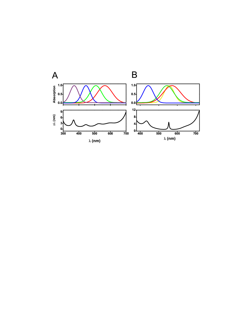
Figure 5: Minimal discrimination error $\Delta\lambda$ as a function of wavelength $\lambda$, obtained from a generalization of Eq. 13 that considers 4 different types of cones. A. Top: Absorption curves of estrilid finch (Hart et al. 2000) with local maxima at wavelengths $\lambda_{i}=368,445,508,565$ nm, and widths $\sigma_{i}=38.58,38.44,52.87,65.8$ nm, respectively. Bottom: Predicted discrimination error, with mean number of photons set to 1000. Parameters $\beta_{i}$ are set to 0.25 for all cones. B. Top: Putative cone fundamentals of a human tetrachromat (Jordan et al. 2010). The additional curve (in yellow) peaks at $\lambda_{y}=555$ nm, and has width $\sigma_{y}=38.51$ nm. Bottom: Predicted discrimination error, with mean number of photons set to 1000. Parameters $\beta_{i}$ are set to 5%, 31.33%, 31.34% and 31.33% for $S,M,Y$, and $L$ cones, respectively.

equidistant from each other (Hart et al. 2000) giving rise to accurate color discrimination abilities that extend further into the ultraviolet spectrum. Four local maxima are visible in $\Delta\lambda$, accounting for each of the 4 absorption curves.

In panel B, we display the results for a putative human tetrachromat, for which the extra cone is hypothesized to lie between the $M$ and $L$ cones, as anomalous subject cDa29 studied by Jordan et al. (2010). In spite of the incorporation of an additional curve, the discrimination ability of this subject is similar to that of normal trichromats. The substantial overlap between $M$ and $L$ absorption curves of trichromats implies that the addition of one more absorption curve in the same wavelength region makes virtually no difference. This does not mean that the putative tetrachromat of Fig. 5B perceives the same color space as trichromats, since the present discussion is restricted to the discrimination of neighboring monochromatic beams. Color space also includes mixtures of wavelengths (see below), and some mixtures, for example the purples obtained by mixing red and blue, are not metameric with any single monochromatic beam. Tetrachromats may perceive many more mixtures that cannot be mapped on the trichromat color space. Our analysis predicts, however, that their ability to discriminate neighboring monochromatic beams remains essentially unaltered.

5.1 Discrimination of spectra composed of mixtures of wavelengths

To extend the previous analysis to the entire color space, the Fisher information should be written as a function of coordinates that describe the chromatic composition of an arbitrary beam $I(\lambda)$. Equation 5 implies that the probability distribution of the absorbed photons $\overrightarrow{K}$ is blind to all aspects of the spectrum $I(\lambda)$ not contained in the vector $\overrightarrow{\alpha}$ defined in Eq. 4. Replacing Eq. 5 in 7, we get

$$J\left(\overrightarrow{\alpha}\right)=\left(\begin{array}[]{ccc}\frac{1}{\alpha_{S}}&0&0\\ 0&\frac{1}{\alpha_{M}}&0\\ 0&0&\frac{1}{\alpha_{L}}\end{array}\right).$$ (14)

The metric tensor is diagonal, so the ellipsoids defining the points at constant distance of a given parameter $\overrightarrow{\alpha}$ have their principal axes aligned with the coordinate axes. The square root of the inverse of $J\left(\overrightarrow{\alpha}\right)$ defines an ellipsoid around each color $\overrightarrow{\alpha}$ where all points are at the same distance from the central point $\overrightarrow{\alpha}$ (Fig. 6).

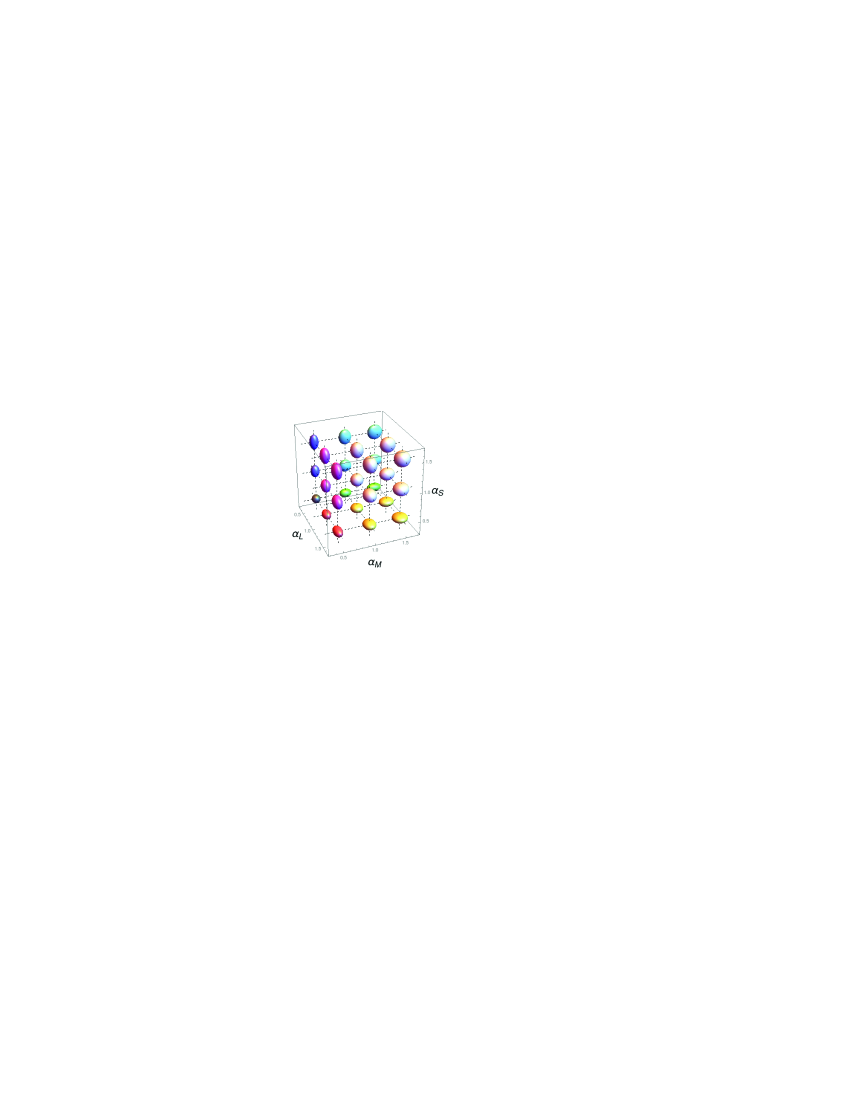
Figure 6: Ellipsoids indicating the regions of space $\overrightarrow{\alpha}$ lying at a fixed distance of each central point.

In order to compare with experimental data, we need to transform the metric tensor of Eq. 14 from the parameter space $\overrightarrow{\alpha}$ to the CIE 1931 $xy$ chromatic space where MacAdam reported the minimal discriminable ellipses. We perform the transformation in two steps. First, we change from $(\alpha_{S},\alpha_{M},\alpha_{L})$ to $(X,Y,Z)$, and then from $(X,Y,Z)$ to the triplet $(x,y,Y)$. So far, the two transformations are invertible. Once we have the Fisher matrix in the space $xyY$, we take the submatrix associated to the components $xy$ alone, in order to compare with MacAdam’s experiment.

Each of the two transformations involves a $C$-matrix defined in Eq. 12. If we call $C_{1}$ the matrix of the first transformation, and $C_{2}$ the one of the second, the two concatenated transformations are implemented by a matrix $C=C_{1}C_{2}$. To calculate $C_{1}$ we analyze the way the color matching functions transform, when passing from $(\alpha_{S},$ $\alpha_{M},\alpha_{L})$ to $(X,Y,Z)$. By fitting a linear transformation between the two, we deduce that

$$\left(\begin{array}[]{c}\alpha_{S}\\ \alpha_{M}\\ \alpha_{L}\end{array}\right)=C_{1}\ \left(\begin{array}[]{c}X\\ Y\\ Z\end{array}\right),\ \ \ \ \ \ \ \ {\rm with}\ \ \ \ C_{1}=\left(\begin{array}[]{ccc}0.038\beta_{S}&-0.043\beta_{S}&0.48\beta_{S}\\ -0.39\beta_{M}&1.17\beta_{M}&0.049\beta_{M}\\ 0.34\beta_{L}&0.69\beta_{L}&-0.076\beta_{L}\end{array}\right).$$

To calculate $C_{2}$, we invert Eq. 1 and find

$$X=Y\ x/y\ \ \ \ \ \ \ \ \ \ \ \ Y=Y\ \ \ \ \ \ \ \ \ \ \ \ Z=Y\ (1-x-y)/y.$$

Using Eq. 12, we obtain

$$C_{2}=\left(\begin{array}[]{ccccc}\frac{Y}{y}&&-\frac{xY}{y^{2}}&&\frac{x}{y}\\ &&&&\\ 0&&0&&1\\ &&&&\\ -\frac{Y}{y}&&-\frac{Y(1-x)}{y^{2}}&&\frac{1-x-y}{y}\end{array}\right).$$

With the resulting matrix $C=C_{1}C_{2}$, we calculate the Fisher tensor in space $xyY$, and then focus on the submatrix corresponding to the first two components. All the coefficients of the obtained $2\times 2$ submatrix are proportional to the luminosity variable $Y$. Hence, the lengths of the principal axes of the ellipses defining the equidistant colors are proportional to $Y^{-1/2}$, and the area is proportional to $1/Y$. Other than this scaling factor, the luminosity variable has no additional effect. Since all other variables appearing in the Fisher tensor are adimensional, the units with which we measure distances in the $xy$ space are $[Y]^{-1/2}$. Here we use MacAdam’s unit of color difference (Wyszecki and Stiles 2000), implying that the distance between each central point and the ellipse measured by MacAdam is unity. In this system, the coordinate $Y$ is adimensional.

In Fig. 7 the ellipses at distance 1 from 31 center points are displayed.

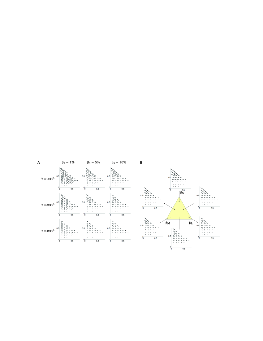
Figure 7: Ellipses obtained by transforming the ellipsoids in Fig. 6. $xy$ CIE chromatic coordinates represented by the horizontal and vertical axes, respectively. A: Dependence of ellipses on parameters $\beta_{S}$ and $Y$. We set $\beta_{M}=\beta_{L}=(1-\beta_{S})/2$. B: Dependence of ellipses on retinal composition, for $Y=2\times 10^{5}$. The triangle represents the accessible area of the space $(\beta_{S},\beta_{M},\beta_{L})$. Indicated panels correspond to $\overrightarrow{{\beta}}=(\beta_{S},\beta_{M},\beta_{L})=(0.8,0.1,0.1)$ (top), $(0.45,0.1,0.45),(0.1,0.1,0.8),(0.1,0.45,0.45),(0.1,0.8,0.1)$ and $(0.45,0.45,0.1)$ as we rotate clockwise. As customary, ellipses are enlarged 10 times in each dimension for better visualization.

In A, $\beta_{S}$ is varied within the physiological range. As $\beta_{S}$ increases (from left to right) the ellipses become smaller, and more compressed along the direction $(1,-1)$. Increasing the value of $Y$ (from top to bottom) shrinks the ellipses.

In B, we display the ellipses for several retinal compositions, without restricting the values of $\beta_{i}$ to the realistic range. In this context, any set of $(\beta_{S},\beta_{M},\beta_{L})$ defines a possible retina, as long as all $\beta_{i}$ are positive, and the three of them sum up to unity. In the space of possible $\overrightarrow{\beta}$ vectors, these conditions define the triangle illustrated in Fig. 7B. As we move along the bottom border of the triangle, we confirm that the relative proportion of $\beta_{M}$ and $\beta_{L}$ does not change the ellipses qualitatively (three bottom panels). Increasing $\beta_{S}$, instead (moving upward) reduces the size of the ellipses in the direction $(1,1)$, and augments them along the direction $(-1,1)$. In other words, increasing the proportion of $\beta_{S}$ helps discriminating blue vs. yellow stimuli, but has a detrimental effect on the discrimination of red vs. green. The ellipses corresponding to the inner area of the triangle smoothly interpolate those at the border.

In order to compare with MacAdam’s experiment, we need to fit the parameters $\beta_{S}$ and $Y$, both kept fixed during the experiment. To do so, we systematically vary $\beta_{S}\in(0,0.1)$ and $Y\in(0,10^{6})$ and compare the theoretical ellipses evaluated at the 25 points measured by MacAdam with the 25 experimental ellipses. The optimal parameters are the ones that make both sets of ellipses maximally similar. To do so, we need a criterion of similarity between ellipses. Two concentric ellipses may differ in their size, their orientation, or their excentricity. In order to evaluate the three aspects simultaneously, and to adequately weigh the relevance of each, we define the distance between two concentric ellipses as the Kullback-Leibler divergence between two Gaussian distributions whose covariance matrices are defined by the tested ellipses. As the two distributions become more and more similar, the two ellipses merge into one another, implying a simultaneous match between size, elongation and excentricity. Averaging over the 25 measured points, $\beta_{S}$ and $Y$ are fitted by minimizing

$$D=\frac{1}{25}\sum_{i=1}^{25}{\rm D}_{KL}\left[{\cal N}({\bf r}_{i},\Sigma_{i}^{th})||{\cal N}({\bf r}_{i},\Sigma_{i}^{e})\right],$$

where the sum runs over the 25 colors tested by MacAdam, ${\rm D}_{KL}$ is the Kullback-Leibler divergence, ${\cal N}({\bf r}_{i},$ $\Sigma)$ is a normal bivariate distribution centered at the colors $\bf{r}_{i}$ where MacAdam performed his experiment, and with covariance matrix $\Sigma$. The supra-index $th$ represents the theoretical matrix, and $e$ the experimental one. The experimental covariance matrix is constructed from the reported ellipses: We calculate the matrix whose eigenvectors are in the directions of the principal axes reported by MacAdam, and whose eigenvalues coincide with the lengths of the principal axes. The theoretical covariance matrix is the inverse of the Fisher information. An analytical form for the Kullback-Leibler divergence for multivariate Gaussian distributions is derived in Duchi (2014). When $D$ is employed as a fitting criterion, the goodness-of-fit may be defined in terms of an $R^{2}$-value defined as $R^{2}=1-D/{\rm D}_{e}$, where ${\rm D}_{e}$ is the average Kullback-Leibler divergence between all experimental ellipses.

In Fig. 8A we see the dependence of $D$ with parameters $\beta_{S}$ and $Y$. The optimal values are $\beta_{S}=2.1\%$ and $Y=184,000$, for which $D=0.36$, and $R^{2}=0.87$.

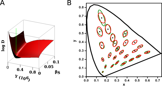
Figure 8: Comparison between theory and experiment. A: Distance $D$ between theoretical and experimental ellipses as a function of parameters $\beta_{S}$ and $Y$. The green vertical line indicates the location of the optimal parameter values $\beta_{S}=2.1\%$ and $Y=184,000$. B: Ellipses measured by MacAdam (green) compared to the ones derived from our theoretical model (red) for the optimal parameters. As customary, each ellipse is enlarged 10 times in each dimension for better visualization.

In Fig. 8B, we see the model is effective in describing the variation of the size, orientation and excentricity of the ellipses throughout the chromatic space. More quantitatively, the obtained $R^{2}$ value implies that the theory explains 87% of the variability of the experimental data.

6 Discussion

Here we derived a metric in color space from a noise model of the representation of color in the brain. Several classical studies have derived the minimal discrimination ellipses from line elements (Wyszecki and Stiles, 2000). Those theories used heuristic arguments to propose a distance in color space. Not being framed in the Fisher geometry, they do not entail a data processing inequality nor a Cramér-Rao bound. The advantage of the Fisher metric is that it brings along a rigorous mathematical framework, first, for deriving the metric from a noise model, and then, for transforming the metric from one space to another. Given the noise model, the Fisher metric is undisputable. Of course, there are many candidate noise models, depending on which neuronal processes are described. The confrontation of the derived Fisher ellipses with experimental data actually provides a systematic way to evaluate the adequacy of alternative noise models.

Here we offer an attempt to perform such confrontation, using one particular noise model based on the sole description of the photon absorption process. We conclude that a simple Poisson model of the statistics of photoreceptor absorption account for $\approx 87$% of the variance of the behavioral results in the $xy$ chromatic space. Our theory also predicts that the minimal discrimination error is inversely proportional to the square root of the light intensity, following a Rose-DeVries law, originally reported in contrast discrimination thresholds at low light intensities (Rose 1948, DeVries 1943), and later confirmed for chromatic discrimination experiments (Rovamo et al 2001). Experiments show that this dependence holds in the low-intensity photopic regime, but loses validity as the light intensity becomes larger (Rovamo et al 2001). Therefore, additional optic or neural color-dependent processing stages not contained in the Poisson photoreceptor model must come into play at high intensities.

In spite of having neglected all subsequent color processing stages beyond absorption, even the voltage variations in the inner segments of photoreceptors, the distances derived from the Fisher approach reproduce a large fraction of the experimental variability. The derived ellipses are only guaranteed to coincide with the measured discrimination error when the Cramér-Rao bound is tight, that is, when further processing stages perform optimally, or at least, they do not introduce additional color-dependent distortions. A priori, there is no reason to believe that such should be the case. The similarity between the theoretical and the experimental results therefore suggests that photon absorption constitutes the crucial stage in the chromatic dependence of color processing ability, and it suffices to explain most of the structure observed in experimental data. All subsequent processing stages either perform optimally or, if they lose information, they do so in a color-independent manner.

The Cramér-Rao bound of Eq. 26 is only valid for unbiased estimators, a more complex formula is required in the biased case (Cover and Thomas, 1991). However, in the presence of achromatic backgrounds (as in all experiments explored here), discrimination errors have been always reported to have zero mean, so we work under the assumption that the nervous system is able to implement at least one unbiased estimator, for which Eq. 26 holds. Different is the case where the target and test stimuli are presented against a chromatic background, where subjects have been reported to bias their estimation of the target stimulus away from the hue of the background (see for example Klaue and Wachtler 2015). In such cases, we suspect that the more complex form of the Cramér-Rao bound should be employed.

The Fisher tensor determines the distance between neighboring colors; the distance between distant colors must be calculated by adding the infinitesimal distances encountered along a specific path. If one of the two colors lies at a border of the chromatic space, the path must be entirely contained inside the space. When the path connecting two colors is short, all the involved infinitesimal distances are obtained from essentially the same Fisher tensor, since the Fisher metric varies smoothly with location. When comparing the theoretical and experimental ellipses, we have assumed that the Fisher distance between the central color and the ellipse could be calculated with a single Fisher tensor: the one of the center. To assess the validity of the approximation, we verified that inside each ellipse the eigenvalues of the theoretical Fisher tensor vary at most 1.27 %, and the inclination angle at most $0.97^{\circ}$ (recall that all depicted ellipses have been enlarged 10 times in each dimension, for better visibility).

We are aware of two other previous studies where chromatic discrimination ability was modeled by information-theoretical methods. The first one (Clark and Skaff, 2009) was based on stronger assumptions as the ones used here, since the properties of chromatic perception were explained in terms of a specific decoding process that takes place (explicitly or implicitly) in the visual system. Our work neither supports nor refutes the proposed decoding, we simply show that it is not strictly required to explain a large fraction of the variance in human discrimination ability. The second study was developed by Zhaoping et al. (2011). Their approach was the starting point for the present study. They also discussed how the Fisher metric varies with mean light intensity. Instead here, we have focused on (a) providing an analytical formula for the monochromatic case, (b) extending the analysis to the whole chromatic space, and (c) discussing the discrimination ability of observers endowed with different retinal compositions.

Chromatic discrimination ability is limited by the imprecision with which neighboring colors are represented in the brain. The stochasticity considered here regards the unpredictability of the exact proportion of photons captured by $S$, $M$ and $L$ cones, given that the three absorption curves overlap with each other. The variance of $K_{i}$ is $Kq_{i}(1-q_{i})$, and is maximal when both $q_{i}$ and $1-q_{i}$ are far from zero. For $M$ and $L$ cones, this condition is met at approximately 550 nm, where both absorption probabilities are high. Human color discrimination error has a local maximum at $\approx$ 550 nm, roughly coinciding with the wavelength where humans perceive maximal luminosity (Sharpe et al. 2005). So far, this coincidence appeared as incidental. An analysis of the equations involved in our study, however, reveals that color discrimination ability is determined by the derivative of the quantal cone fundamentals: The larger the derivative, the larger the value of the Fisher information (Dayan and Abbott, 2001). Since $L$ and $M$ cone fundamentals are very similar, and given that the variance is particularly large at $\approx$ 550 nm, the two maxima cannot be separated apart, and discrimination error peaks at a wavelength that is approximately the average of the wavelengths where $L$ and $M$ absorption curves reach their maxima. The coincidence, hence, is grounded on the mathematical properties of the Fisher information. If the number of $S$ cones is large enough, a local maximum in discrimination error is also achieved at the wavelength where the S-cone absorption curve peaks, $\approx$ 450 nm. Moreover, the theory also predicts how discrimination ability varies with retinal composition, suggesting that the variability in anatomical properties of different observers may account for the variability in the experimental data.

Throughout our work, we have only considered cones, although rod absorption is also modulated by wavelength. By a simple extension of our analysis, it is also possible to include rods in the evaluation of chromatic discrimination ability. However, since rods and cones have different luminosity sensitivity, the comparison with behavioral data should be performed with experiments where the total light intensity was controlled. The parameters $\beta_{i}$ scaling the relevance of each photoreceptor should also include a factor accounting for the different cross sections of rods and cones, and their differential sensitivity depending on the total luminosity. The analysis presented here is only valid for photopic illumination conditions (as reported by the experiments) where rods are assumed to be saturated. Extensions to other models, including rods or other optical and neural processes, are possible. Results can be expressed in the classical color spaces employed here, through the transformation formulas of Sect. 4.

Appendix

A1: Transformations of the light spectrum leading to representations of color

From the physical point of view, the spectrum $I(\lambda)$ provides a complete characterization of a light beam. The space of all possible spectra has infinite dimensions. Color matching experiments performed by Helmholtz and Young proved that by adjusting the intensity of three monochromatic sources of fixed wavelengths, human trichromats construct a beam that they perceive as visually indistinguishable from a target light source of arbitrary spectrum. Hence, the human visual system projects the high-dimensional space of all possible spectra onto three dimensions (Fig. 9).

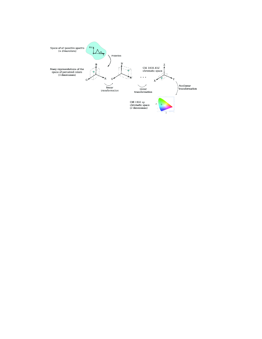
Figure 9: Transformations between different representations of the composition of a light beam. Top: The most complete representation is the spectrum $I(\lambda)$, specifying the energy density in each wavelength. The space of all possible spectra has infinite dimensions. Middle: The human visual system can only perceive 3 dimensions. The projection from the space of spectra to the space of chromatic perceptions is linear (Grassmann’s law). There are many representations of the 3-dimensional space perceived by humans. One of them is the CIE 1931 $XYZ$ color space (middle bottom). Each spectrum at the top projects to a single point in the three-dimensional space by means of a non-invertible transformation. Bottom: The CIE 1931 $xy$ chromatic space is a nonlinear transformation of the CIE 1931 $XYZ$ space that eliminates the luminosity dimension, and only keeps variations in hue and saturation. Each point of the three-dimensional space maps onto a point in the $xy$ space.

When the target light source is monochromatic and has wavelength $\lambda$, the three intensities required to construct the mixture define the color matching functions $\bar{b}(\lambda),\bar{g}(\lambda)$ and $\bar{r}(\lambda)$, whose functional shape depends on the wavelengths of the three sources than comprise the mixture. The matching operation is linear, implying that the visual appearance of an arbitrary spectrum $I(\lambda)$ is governed by three numbers, defined as

$$\begin{array}[]{lll}B=\int I(\lambda)\bar{b}(\lambda)\ {\rm d}\lambda,&G=\int I(\lambda)\bar{g}(\lambda)\ {\rm d}\lambda,&R=\int I(\lambda)\bar{r}(\lambda)\ {\rm d}\lambda.\end{array}$$ (15)

If the wavelengths of the three fixed light sources are varied, the shape of the color matching functions changes. Different $(R,G,B)$ representations have thus appeared, depending on the chosen wavelengths. In fact, any invertible linear transformation of one set of coordinates $(R,G,B)$ yields a new set of coordinates $(R^{\prime},G^{\prime},B^{\prime})$ equally valid, represented in Fig. 9 as one of the coordinate systems in the middle column. The new coordinates can also be obtained from integrals like Eq. 15, but with new functions $\bar{b}^{\prime}(\lambda),\bar{g}^{\prime}(\lambda),\bar{r}^{\prime}(\lambda)$, derived from a linear transformation of the old functions. In 1931, the International Commission on Illumination (CIE, for its initial in French) selected a particular set of coordinates $(X,Y,Z)$, associated with specific color matching functions usually notated as $\bar{x}(\lambda),\bar{y}(\lambda),\bar{z}(\lambda)$ (Wyszecki and Stiles, 2000).

A2: Poisson absorption models

In this appendix, we derive Eqs. 2 and 5. Repeated use is made of the formulas

$${\rm{\bf Binomial:}}\ \ (a+b)^{n}=\sum_{j=0}^{n}\frac{n!}{j!(n-j)!}\ a^{j}\ b^{n-j};\ \ \ \ {\rm{\bf Multinomial:}}\ \ \left(\sum_{i=1}^{k}a_{i}\right)^{n}=n!\ \sum_{j_{1},\dots,j_{k}}\prod_{\ell=1}^{k}\frac{a_{\ell}^{j_{\ell}}}{j_{\ell}!},$$

where the sum of the multinomial theorem runs over all sets of integers $\{j_{1},\dots,j_{k}\}$ fulfilling the conditions $0\leq j_{\ell}\leq n$ and $n=j_{1}+\dots+j_{k}$.

Monochromatic light source of fixed intensity

When a photon of wavelength $\lambda$ impinges on the retina under central photopic illumination conditions, four outcomes are possible: The photon may be detected by a cone of type $S$, $M$ or $L$, or it may pass undetected. The probability of each outcome depends on the fraction of $S$, $M$ and $L$ cones that tile the retina and on the probability that each cone absorbs a photon of wavelength $\lambda$, also called the spectral sensitivity of each cone. Once these parameters are known, from the statistical point of view, illuminating the retina with $I_{0}$ photons of wavelength $\lambda$ is equivalent to randomly distributing $I_{0}$ balls into 4 boxes whose cross sections depend on the wavelength $\lambda$. The probability that $N_{S},N_{M}$ and $N_{L}$ fall on $S,M$ and $L$-cones respectively, and that $N_{0}$ do not fall on cones is

$$P(\overrightarrow{N}|I_{0})=I_{0}!\prod_{i\in\{S,M,L,0\}}\frac{\beta_{i}^{N_{i}}}{N_{i}!},$$ (16)

where $\overrightarrow{N}=(N_{S},N_{M},N_{L})$. The components $N_{S},N_{M},N_{L},N_{0}$ are not all independent, since they must sum up to $I_{0}$. Therefore, $N_{0}$ is a shorthand notation for $N_{0}=I_{0}-N_{S}-N_{M}-N_{L}$.

When $N_{i}$ photons reach a cone of type $i$, the probability that $K_{i}$ of them are absorbed is a binomial distribution with absorption probability $h_{i}(\lambda)$ (Fig.2),

$$P(K_{i}|N_{i})=\frac{N_{i}!}{K_{i}!(N_{i}-K_{i})!}\ h_{i}(\lambda)^{K_{i}}\ [1-h_{i}(\lambda)]^{N_{i}-K_{i}},\ \ \ {\rm for\ \ }i\in\{S,M,L\}.$$ (17)

When these two processes are coupled sequentially, the fate of each photon is decided through the processes depicted in Fig. 10.

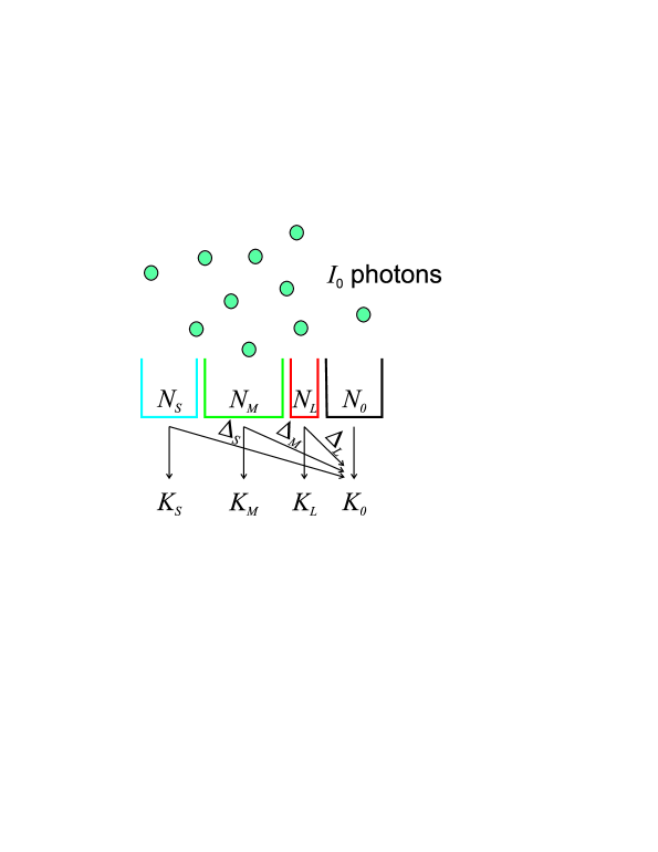
Figure 10: $I_{0}$ photons of wavelength $\lambda$ fall on $S$, $M$ or $L$ cones (colored boxes), or miss cones altogether (black box). Each of the $N_{i}$ photons that fall on cones of type $i$ may either be absorbed (and become one of the $K_{i}$ photons absorbed by a photoreceptor of type $i$), or pass unabsorbed (and become one of the $\Delta_{i}$ photons not absorbed by a cone of type $i$). The total number of photons absorbed by a cone of type $i$ is $K_{i}=N_{i}-\Delta_{i}$, and the number of photons that remain unabsorbed is $K_{0}=N_{0}+\Delta_{S}+\Delta_{M}+\Delta_{L}$. The process that transforms the $K$ impinging photons into $(N_{S},N_{M},N_{L},N_{0})$ is governed by the multinomial distribution of Eq. 16, and the one that transforms $N_{i}$ into $K_{i}$, by the binomial of Eq. 17.

The probability that $K_{S},K_{M},K_{L}$ photons are absorbed by cones $S,M,L$ and that $K_{0}$ pass undetected is

$$P(\overrightarrow{K}|I_{0},\lambda)=\sum_{{\bf N}>{\bf K}}P(\overrightarrow{N}|I_{0},\lambda)\ \prod_{i\in\{S,M,L\}}\ P(K_{i}|N_{i}),$$ (18)

where the sum ranges over all vectors $\overrightarrow{N}=(N_{S},N_{M},N_{L})$ that fulfill the conditions $N_{S}\geq K_{S},N_{M}\geq K_{M},N_{L}\geq K_{L}$ and $N_{S}+N_{M}+N_{L}\leq I_{0}$. Replacing Eqs. 16 and 17 in Eq. 18, defining the scaled absorption probabilities $q_{i}(\lambda)=\beta_{i}h_{i}(\lambda)$, for $i\in\{S,M,L\}$, and $q_{0}(\lambda)=1-q_{S}(\lambda)-q_{M}(\lambda)-q_{L}(\lambda)$ and the the numbers $\Delta_{S},\Delta_{M}$ and $\Delta_{L}$ of lost photons (see Fig. 10)

$$\begin{array}[]{ccc}\Delta_{S}=N_{S}-K_{S},&\Delta_{M}=N_{M}-K_{M},&\Delta_{L}=N_{L}-K_{L},\end{array}$$

we get, after some algebraic manipulations,

$$P(\overrightarrow{K}|I_{0},\lambda)=I_{0}!\ \prod_{i\in\{S,M,L,0\}}\frac{q_{i}(\lambda)^{K_{i}}}{K_{i}!}.$$ (19)

The derivation involved the use of the binomial theorem three times. The composition of the multinomial process of Eq. 16 and the binomial of Eq. 17 yields another multinomial distribution governed by the scaled absorption probabilities, combining the parameters governing the two processes in play. In Eq. 19, the variables $K_{S},K_{M}$ and $K_{L}$ are not independent, since the distribution also includes a factor that depends on $K_{0}=I_{0}-K_{S}-K_{M}-K_{L}$.

Monochromatic light source of variable intensity

If the total number of photons $I_{0}$ of wavelength $\lambda$ is a stochastic variable governed by a Poisson distribution of mean $I$

$$P[I_{0}|I]={\rm e}^{-I}\ \frac{I^{I_{0}}}{I_{0}!},$$ (20)

then the probability of the absorbed photons is

$$P[\overrightarrow{K}|\lambda,I]=\sum_{I_{0}=0}^{+\infty}P(\overrightarrow{K}|I_{0},\lambda)\ P[I_{0}|I].$$ (21)

Replacing Eq. 19 and 20 in Eq. 21, and after some algebraic manipulations, we arrive at Eq. 2. A light source with variable intensity, hence, gives rise to absorbed photon counts $K_{S},K_{M},K_{L}$ that are independent from one another.

Light sources of arbitrary spectrum

We now consider a light source composed of photons of $r$ different wavelengths $\lambda_{j}$, where $j$ ranges between $1$ and $r$. The mean number of photons of the different wavelengths defines an $r$-dimensional vector $\overrightarrow{I}=(I(\lambda_{1}),\dots,I(\lambda_{r}))$. There are many ways in which $S$ cones can absorb $K_{S}$ photons: All the $K_{S}$ photons may have the same wavelength $\lambda_{1}$, half of them may have wavelength $\lambda_{1}$ and the other half wavelength $\lambda_{2}$, etc. Here we consider all the possibilities. We define $G_{S}^{j}$ as the number of photons of wavelength $\lambda_{j}$ absorbed by cones $S$, and arrange these numbers in $r$-dimensional vectors

$$\begin{array}[]{ccc}{\bf G}_{S}=(G_{S}^{1},\dots,G_{S}^{r}),&{\bf G}_{M}=(G_{M}^{1},\dots,G_{M}^{r}),&{\bf G}_{L}=(G_{L}^{1},\dots,G_{L}^{r}).\end{array}$$

If the total numbers of absorbed photons are $K_{S},K_{M}$ and $K_{L}$, the components of the three vectors defined above must sum up to these values, that is,

$$\begin{array}[]{ccc}\sum_{j=1}^{r}G_{S}^{j}=K_{S},&\sum_{j=1}^{r}G_{M}^{j}=K_{M},&\sum_{j=1}^{r}G_{L}^{j}=K_{L}.\end{array}$$ (22)

We call ${\cal U}_{S}$, ${\cal U}_{M}$ and ${\cal U}_{L}$ the sets of all vectors ${\bf G}_{S}$, ${\bf G}_{M}$ and ${\bf G}_{L}$ whose components are non-negative integers fulfilling Eqs. 22. Mathematically, for $i\in\{S,M,L\}$,

$${\cal U}_{i}=\{{\bf G}_{i}/G_{i}^{j}\geq 0\ \forall j\ \&\ \sum_{j=1}^{r}G_{i}^{j}=K_{i}\},$$

The probability of cones $S,M$ and $L$ of absorbing $\overrightarrow{K}$ photons can be written in terms of the sum of all possible spectral compositions of the absorbed photons, namely,

$$P(\overrightarrow{K}|\vec{I}\ )=\sum_{{\bf G}_{S}\in{\cal U}_{S}}\sum_{{\bf G}_{M}\in{\cal U}_{M}}\sum_{{\bf G}_{L}\in{\cal U}_{L}}\prod_{j=1}^{r}P[G_{S}^{j},G_{M}^{j},G_{L}^{j}|I(\lambda_{j})],$$ (23)

where the probability $P[G_{S}^{j},G_{M}^{j},G_{L}^{j}|I(\lambda_{j})]$ in the right-hand side of Eq. 23 is the same as the one of Eq. 2, but is now evaluated in a $G$-vector (as opposed to a $K$-vector). The sums represent the fact that many combination of wavelengths may contribute to the same $\overrightarrow{K}$.

Replacing Eq. 2 in Eq. 23, and using the multinomial theorem, we get

$$P(\overrightarrow{K}|\vec{I})=\prod_{\ell\in\{S,M,L\}}\frac{\exp\left[-\sum_{i=1}^{r}I(\lambda_{i})q_{\ell}(\lambda_{i})\right]}{K_{\ell}!}\ \left[\sum_{j=1}^{r}I(\lambda_{j})q_{\ell}(\lambda_{j})\right]^{K_{\ell}}.$$ (24)

Defining the coordinates $(\alpha_{S},\alpha_{M},\alpha_{L})$

$$\alpha_{i}=\sum_{j=1}^{r}I(\lambda_{j})q_{i}(\lambda_{j}),\ \ \ {\rm for}\ i\in\{S,M,L\},$$ (25)

Eq. 24 yields Eq. 5. If the spectrum contains a continuum of wavelengths $\lambda$ with mean spectral energy $I(\lambda)$, the calculations performed here remain unchanged, except for the fact that the coefficients $\alpha_{i}$ must be defined in terms of integrals (compare Eq. 4 and 25).

A3: The Fisher geometry

Here, the properties of the light beam that are relevant to color discrimination are represented by a vector of parameters $\overrightarrow{\alpha}=(\alpha_{1},\dots,\alpha_{d})$. In this appendix, the parameter $\overrightarrow{\alpha}$ is not necessarily defined by Eqs. 4. For example, when applied to experiments performed with monochromatic beams, we can take $d=1$, and $\overrightarrow{\alpha}$ equal to the wavelength $\lambda$ (or equivalently, any invertible function of the wavelength). In the case of mixtures, we may take $d=3$, and $\overrightarrow{\alpha}$ defined by Eqs. 4, or equivalently, as $\overrightarrow{\alpha}=(X,Y,Z)$. We may also consider $d=2$ and $\overrightarrow{\alpha}=(x,y)$.

If the probability distribution of a random variable $\overrightarrow{K}$ depends on the parameter $\overrightarrow{\alpha}$, a notion of distance can be defined in the $\overrightarrow{\alpha}$ space, quantifying the effect of changing $\overrightarrow{\alpha}$ on $P(\overrightarrow{K}|\overrightarrow{\alpha})$. It may well be the case that in certain regions of the $\overrightarrow{\alpha}$ space, a displacement of the parameter in a certain amount ${\rm d}\overrightarrow{\alpha}$ changes the distribution $P(\overrightarrow{K}|\overrightarrow{\alpha})$ radically, whereas in other regions the same displacement hardly has an effect. In these circumstances, distances in the $\overrightarrow{\alpha}$ space vary from point to point: The same displacement ${\rm d}\overrightarrow{\alpha}$ corresponds to a large distance in the first case, and to small one in the second. The Fisher information introduced in Eq. 7 defines a metric tensor that gives rise to a notion of distance in parameter space: the length of a vector is given by Eq. 9, and the distance between two neighboring vectors $\overrightarrow{\alpha}^{a}$ and $\overrightarrow{\alpha}^{b}$ is the length of $\overrightarrow{\alpha}^{a}-\overrightarrow{\alpha}^{b}$. The Cramér-Rao bound relates the Fisher tensor to the accuracy with which the random variable $\overrightarrow{K}$ can be used to estimate the parameter $\overrightarrow{\alpha}$. If the Fisher information is large, sampling $\overrightarrow{K}$ can provide a good estimate of $\overrightarrow{\alpha}$, if an efficient decoding procedure is used. A low Fisher information, in contrast, implies that $P(\overrightarrow{K}|\overrightarrow{\alpha})$ hardly varies with $\overrightarrow{\alpha}$ and therefore, it is impossible to make (on average) a good guess of the value of $\overrightarrow{\alpha}$ by sampling $\overrightarrow{K}$, not even with an optimal decoding procedure. Formally, this means that the mean quadratic error of any unbiased estimator $\hat{\overrightarrow{\alpha}}(\overrightarrow{K})$ of the parameter $\overrightarrow{\alpha}$ is bounded from below. We define the mean quadratic error as a $d\times d$ matrix $E$, with elements

$$E_{ij}(\overrightarrow{\alpha})=\left\langle\left[\hat{\alpha}_{i}(\overrightarrow{K})-\alpha_{i}\right]\left[\hat{\alpha}_{j}(x)-\alpha_{j}\right]\right\rangle_{P\left(\overrightarrow{K}|\overrightarrow{\alpha}\right)}.$$

The Cramér-Rao bound states that

$$E(\overrightarrow{\alpha})\cdot J(\overrightarrow{\alpha})\geq\mathbbm{1},$$ (26)

where $\mathbbm{1}$ is the identity matrix, and the inequality implies that all the eigenvalues of the matrix $E\cdot J$ cannot be smaller than unity. The Cramér-Rao bound of Eq. 26 can also be expressed as $E\geq J^{-1}$. Therefore, $J^{-1}$ is the minimal mean quadratic estimation error. The larger the information, the smaller the error, and vice versa. The bound expressed in Eq. 26 is only valid for unbiased estimators, a more complex formula is required in the biased case (Cover and Thomas, 1991).

In Sect. 2, several representations of the composition of a light beam were introduced. One may, for example, represent the light beam with the spectrum $I(\lambda)$, or with specific coordinates $RGB$, or with the CIE 1931 $XYZ$, or the reduced $xy$. Assume that new coordinates $\overrightarrow{\alpha}^{\prime}$ are defined from old coordinates $\overrightarrow{\alpha}$ by means of a transformation $\overrightarrow{F}$ (see Eq. 10). If the elements of the Fisher information matrix for the representation $\overrightarrow{\alpha}$ are known, one may calculate their value in the representation $\overrightarrow{\alpha^{\prime}}$. The transformation must be such as to preserve scalar products. If $\overrightarrow{\alpha}^{a}$ and $\overrightarrow{\alpha}^{b}$ are two infinitesimal displacements from the vector $\overrightarrow{\alpha}$, the transformed infinitesimal displacements $\overrightarrow{\alpha}^{\prime a}$ and $\overrightarrow{\alpha}^{\prime b}$ are defined from the first order expansion of $\overrightarrow{F}$,

$$\overrightarrow{F}(\overrightarrow{\alpha}+\overrightarrow{\alpha}^{a}) \approx \overrightarrow{F}(\overrightarrow{\alpha})+\left[(\overrightarrow{\alpha}^{a})^{T}\overrightarrow{\nabla}\right]\overrightarrow{F}(\overrightarrow{\alpha})\equiv\overrightarrow{\alpha}^{\prime}+\overrightarrow{\alpha}^{\prime a}$$

$$\overrightarrow{F}(\overrightarrow{\alpha}+\overrightarrow{\alpha}^{b}) \approx \overrightarrow{F}(\overrightarrow{\alpha})+\left[(\overrightarrow{\alpha}^{b})^{T}\overrightarrow{\nabla}\right]\overrightarrow{F}(\overrightarrow{\alpha})\equiv\overrightarrow{\alpha}^{\prime}+\overrightarrow{\alpha}^{\prime b}$$

Therefore, $\overrightarrow{\alpha}^{\prime i}=\left[(\overrightarrow{\alpha}^{i})^{T}\overrightarrow{\nabla}\right]\overrightarrow{F}(\overrightarrow{\alpha})$, for $i\in\{a,b\}$. Preserving the scalar product means that

$$(\overrightarrow{\alpha}^{a})^{T}\ J(\overrightarrow{\alpha})\ \overrightarrow{\alpha}^{b}=(\overrightarrow{\alpha}^{\prime a})^{T}\ J^{\prime}(\overrightarrow{\alpha}^{\prime})\ \overrightarrow{\alpha}^{\prime b}.$$

Since the displacements $\overrightarrow{\alpha}^{a}$ and $\overrightarrow{\alpha}^{b}$ are arbitrary, we arrive at Eqs. 11 and 12. In general, the matrix $C$ depends on the parameter $\overrightarrow{\alpha}$. Only if $\overrightarrow{F}$ is a linear transformation, $C$ reduces to a constant matrix.

References

1. Abbot, L. F., & Dayan, P. (1999). The effect of correlated variability on the accuracy of a population code. Neural Computation 11, 91-101.

2. Amari, S.-I., & Nagaoka, H. (2000). Methods in information Geometry. Providence RI: American Mathematical Society.

3. Brunel N., & Nadal J. P. (1998). Mutual information, Fisher information and population coding. Neural Computation 10(7), 1731-1757.

4. Clark, J.J., & Skaff, S. (2009). A spectral theory of color perception. Journal of the Optical Society of America 26(12), 2488-2502.

5. Cover, T.M., & Thomas J. A. (1991). Elements of Information Theory. New York: Wiley.

6. Cramér, H. (1946). A contribution to the theory of statistical estimation, Scandinavian Actuarial Journal 1946(1), 458-463.

7. Dayan, P., & Abbot, L. F. (2001). Theoretical Neuroscience. Computational and Mathematical Modeling of Neural Systems. Cambridge: MIT Press.

8. DeVries, H. L. (1943). The quantum character of light and its bearing upon threshold of vision, the differential sensitivity and the visual acuity of the eye. Physica 10: 553-564.

9. Duchi, J. C. (2014). Derivations for Linear Algebra and Optimization. Resource document. http://ai. stanford.edu/j̃duchi/projects/general_notes.pdf. Accessed Jan 2016.

10. Ganguli, D. & Simoncelli, E. P., (2014). Efficient Sensory Encoding and Bayesian Inference with Heterogeneous Neural Populations. Neural Computation 26(19), 2103-2134.

11. Hart, N. S., Partridge, J. C., Bennet, A. T. D., & Cuthill, I.C. (2000). Visual pigments, cone oil droplets and ocular media in four species of estrildid finch. Journal of Comparative Physiology A 186, 681-694.

12. Hofer, H., Carroll, J., Neitz, J., Neitz, M., & Williams, D. R. (2005). Organization of the Human Trichromatic Cone Mosaic. Journal of Neuroscience, 25(42), 9669-9679.

13. Jordan, G., Deeb, S. S., Bosten, J. M., & Mollon, J. D. (2010). The dimensionality of color vision in carriers of anomalous trichromacy. Journal of Vision 8(10), 1-19.

14. Klaue, S., & Wachtler. T. (2015). Tilt in color space: Hue changes induced by chromatic surrounds. Journal of Vision 15(13): 17, 111.

15. MacAdam, D. L. (1942). Visual Sensitivities to Color Differences in Daylight. Journal of the Optical Society of America 32(5), 247-274.

16. Pokorny, J., & Smith, V. C. (1970). Wavelength discrimination in the presence of added chromatic fields. Journal of the Optical Society of America 60(4), 562-569.

17. Roorda, A., & Williams, D. R. (1999). The arrangement of the three cone classes in the living human eye. Nature 397, 520-522.

18. Rose, A. (1948) The sensitivity performance of the human eye on an absolute scale. Journal of the Optical Society of America 28:196-208.

19. Rovamo, J. M., Kankaanpää, M. I., & Hallikainen, J. (2001) Spatial neural modulation transfer function for human foveal visual system for equiluminous chromatic gratings. Vision Research 41:1659-1667.

20. Sharpe, L. T., Stockman, A., Jagla, W., & Jägle, H. (2005). A luminous efficiency function $V^{*}(\lambda)$ for daylight adaptation. Journal of Vision 5, 948-968.

21. Seung, H. S., & Sompolinsky, H. (1993). Simple models for reading neuronal population codes. PNAS USA 90: 10749-10753.

22. Stockman, A., & Brainard, D. H. (2009). Color vision mechanisms, in Bass, M. (ed.) OSA Handbook of Optics, New York: McGraw-Hill.

23. von Helmholtz, H. (1896). Handbuch der physiologischen Optik. Leipzig: Voss.

24. Wei, X. X., & Stocker, A. A. (2015). A Bayesian observer model constrained by efficient coding can explain ’anti-Bayesian’ percepts. Nature Neuroscience 18, 1509-1517.

25. Wright, W. D., & Pitt, F. H. G. (1934). Hue discrimination in normal colour vision. Proceedings of the Physical Society 46, 459-473.

26. Wyszecki, G., & Stiles, W. S. (2000). Color Science: Concepts and Methods, Quantitative Data and Formulae. New York: Wiley Interscience.

27. Zhaoping, L., Geisler, W. S., & May, K. A. (2011). Human Wavelength Discrimination of Monochromatic Light Explained by Optimal Wavelength Decoding of Light of Unknown Intensity. PLoS ONE 6(5), e19248. doi:10.1371/journal.pone. 0019248.