Nonparametric adaptive estimation of order 1 Sobol indices in stochastic models, with an application to Epidemiology

Abstract

Global sensitivity analysis is a set of methods aiming at quantifying the contribution of an uncertain input parameter of the model (or combination of parameters) on the variability of the response. We consider here the estimation of the Sobol indices of order 1 which are commonly-used indicators based on a decomposition of the output’s variance. In a deterministic framework, when the same inputs always give the same outputs, these indices are usually estimated by replicated simulations of the model. In a stochastic framework, when the response given a set of input parameters is not unique due to randomness in the model, metamodels are often used to approximate the mean and dispersion of the response by deterministic functions. We propose a new non-parametric estimator without the need of defining a metamodel to estimate the Sobol indices of order 1. The estimator is based on warped wavelets and is adaptive in the regularity of the model. The convergence of the mean square error to zero, when the number of simulations of the model tend to infinity, is computed and an elbow effect is shown, depending on the regularity of the model. Applications in Epidemiology are carried to illustrate the use of non-parametric estimators.

Keywords: Sensitivity analysis in a stochastic framework; Sobol indices of order 1; adaptive non-parametric inference; warped wavelets; model selection; applications to epidemiology; SIR model; spread of the Hepatitis Virus C among drug users.
MSC2010: 49Q12; 62G08; 62P10.

1 Introduction

Sensitivity analysis is widely used for modelling studies in public health, since the number of parameters involved is often high (see e.g. [31, 36] and references therein). It can be applied to a variety of problems, and we focus here on the question of evaluating the impact of input parameters on an output of a model. If we assume that the output of the model, $y\in\mathbb{R}$, depends on $p\in\mathbb{N}$ input parameters $x=(x_{1},...x_{p})\in\mathbb{R}^{p}$ through the relation $y=f(x)$, we are interested here in evaluating how the parameter $x_{\ell}$, for $\ell\in\{1,\dots,p\}$ affects $y$. The vector $x$ of the input parameters can be considered as a realisation of a set of random variables $X=(X_{1},...X_{p})$, with a known distribution and with possibly correlated components. Also, sensitivity analyses in epidemiology deal with deterministic models although in many cases, randomness and nuisance parameters have to be included, which is one of the goal of the present paper.

In public health, most of the studies on sensitivity analysis are performed by letting the input parameters vary on a deterministic grid, or by sampling all parameters from a prior probability distribution [3]. However, there exist other ways of measuring the influence of the inputs on the output. In this article, we are interested in Sobol indices [28], which are based on an ANOVA decomposition (see [27, 16, 17] for a review). Denoting by $Y=f(X)$ the random response, the first order Sobol indices can be defined for $\ell\in\{1,\dots,p\}$ by

$$S_{\ell}=\frac{\mbox{Var}\big{(}\mathbb{E}[Y\ |\ X_{\ell}]\big{)}}{\mbox{Var}(Y)}.$$ (1.1)

This index represents the fraction of the variance of the output $Y$ due to the input $X_{\ell}$. Several numerical procedures to estimate the Sobol indices have been proposed, in particular by Jansen [19] (see also [26, 27]). These estimators, that we recall in the sequel, are based on Monte-Carlo simulations of $(Y,X_{1}\dots X_{p})$.

The literature focuses on deterministic relations between the input and output parameters. In a stochastic framework where the model response $Y$ is not unique for given input parameters, few works have been done, randomness being usually limited to input variables. Assume that:

$$Y=f(X,\varepsilon),$$ (1.2)

where $X=(X_{1},\dots X_{p})$ still denotes the random variables modelling the uncertainty of the input parameters and where $\varepsilon$ is a noise variable. In this paper, we will assume that $f$ (and hence $Y$) is bounded by $M>0$. When noise is added in the model, the classical estimators do not always work: $Y$ can be very sensitive to the addition of $\varepsilon$. Moreover, this variable is not always controllable by the user.

When the function $f$ is linear, we can refer to [12]. In the literature, meta-models are used: approximating the mean and the dispersion of the response by deterministic functions allows to come back to the classical deterministic framework (e.g. Janon et al. [18], Marrel et al. [23]). We study here another point of view, which is based on the non-parametric statistical estimation of the term $\mbox{Var}\big{(}\mathbb{E}[Y\ |\ X_{\ell}]\big{)}$ appearing in the numerator of (1.1). Approaches based on the Nadaraya-Watson kernel estimator have been proposed by Da Veiga and Gamboa [10] or Solís [29]. We propose here a new approach based on warped wavelet decompositions introduced by Kerkyacharian and Picard [20]. An advantage of these non-parametric estimators is that their computation requires less simulations of the model. For Jansen estimators, the number of calls of $f$ required to compute the sensitivity indices is $n(p+1)$, where $n$ is the number of independent random vectors $(Y^{i},X^{i}_{1},\dots X^{i}_{p})$ ($i\in\{1,\dots n\}$) that are sampled for the Monte-Carlo procedure, making the estimation of the sensitivity indices time-consuming for sophisticated models with many parameters.

In Section 2, we present the non-parametric estimators of the Sobol indices of order 1 in the case of the stochastic model (1.2) and study their convergence rates. The approximation of $\mbox{Var}\big{(}\mathbb{E}[Y\ |\ X_{\ell}]\big{)}$ is very important to obtain the speed of convergence. When the conditional expectation is estimated by a Nadaraya-Watson kernel estimator, these results have been obtained by Solís [29] and Da Veiga and Gamboa [10]. The use of wavelets for estimating the conditional expectation in Sobol indices is new to our knowledge. Wavelet estimators are more tractable than kernel estimators in that we do not have to handle approximations of quotients. We derive the convergence rate for the estimator based on wavelets, using ideas due to Laurent and Massart [21] who considered estimation of quadratic functionals in a Gaussian setting. Because we are not necessarily in a Gaussian setting here, we rely on empirical processes and use sophisticated technology developed by Castellan [5]. Contrarily to the kernel estimators for which convergence rates rely on assumptions on the joint distribution of $Y$ and of $X_{1},\dots X_{p}$, we have an upper-bound for the convergence rates that depend on the regularity of the output $Y$ with respect to the inputs $X_{1},\dots X_{p}$. Moreover, our estimator is adaptive and the exact regularity does not need to be known to calibrate our non-parametric wavelet estimator. Since we estimate covariance terms, we obtain elbow effects: there is a threshold in the regularity defining two different regimes with different speeds of convergence for the estimator. In our case, this allows us to recover convergence rates in $1/n$ when the model exhibits sufficient regularities. Further discussion is carried in the body of the article. These estimators are then computed and compared for toy examples introduced by Ishigami [15].

In Section 3, we then address models from Epidemiology for which non-parametric Sobol estimators have never been used to our knowledge. First, the stochastic continuous-time SIR model is considered, in which the population of size $N$ is divided into three compartments: the susceptibles, infectious and removed individuals (see e.g. [1] for an introduction). Infections and removals occur at random times whose laws depend on the composition of the population and on the infection and removal parameters $\lambda$ and $\mu$ as input variables. The output variable $Y$ can be the prevalence or the incidence at a given time $T$ for instance. $Y$ naturally depends on $\lambda$, $\mu$ and on the randomness underlying the occurrence of random times. Second, we consider a stochastic multi-level epidemic model for the transmission of Hepatitis C virus (HCV) among people who inject drugs (PWID) that has been introduced by Cousien et al. [8, 9]. This model describes an individual-based population of PWID that is structured by compartments showing the state of individuals in the heath-care system and by a contact-graph indicating who injects with whom. Additionally the advance of HCV in each patient is also taken into account. The input variables are the different parameters of the model. Ouputs depend on these inputs, on the randomness of event occurrences and on the randomness of the social graph. We compare the sensitivity analysis performed by estimating the Sobol indices of order 1 with the naive sensitivity analysis performed in [8, 9] by letting the parameters vary in an a priori chosen windows.

In the sequel, $C$ denotes a constant that can vary from line to line.

2 A non-parametric estimator of the Sobol indices of order 1

Denoting by $V_{\ell}=\mathbb{E}\big{(}\mathbb{E}^{2}(Y\ |\ X_{\ell})\big{)}$, we have:

$$S_{\ell}=\frac{V_{\ell}-\mathbb{E}(Y)^{2}}{\mbox{Var}(Y)},$$ (2.1)

which can be approximated by

$$\widehat{S}_{\ell}=\frac{\widehat{V}_{\ell}-\bar{Y}^{2}}{\widehat{\sigma}^{2}_{Y}}$$ (2.2)

where

$$\bar{Y}=\frac{1}{n}\sum_{j=1}^{n}Y_{j}\mbox{ and }\widehat{\sigma}^{2}_{Y}=\frac{1}{n}\sum_{j=1}^{n}(Y_{j}-\bar{Y})^{2}$$

are the empirical mean and variance of $Y$. We can think of several approximations $\widehat{V}_{\ell}$ of $V_{\ell}$, for example, based on Nadaraya-Watson and on warped wavelet estimators. At an advanced stage of this work, we learned that the Nadaraya-Watson-based estimator of Sobol indices of order 1 had also been proposed and studied in the PhD of Solís [29]. Using a result on estimation of covariances by Loubes et al. [22], they obtain an elbow effect. However their estimation is not adaptive, and requires the knowledge of the regularity of the joint density function of $(X_{\ell},Y)$. For the warped wavelet estimator, we propose a model selection procedure based on a work by Laurent and Massart [21] to make the estimator adaptive.

2.1 Definitions

Assume that we have $n$ independent couples $(Y^{i},X_{1}^{i},\dots X_{p}^{i})$ in $\mathbb{R}\times\mathbb{R}^{p}$, for $i\in\{1,\dots,n\}$, generated by (1.2).

Our wavelet estimator is based on a warped wavelet decomposition of$\mathbb{E}(Y\,|\,X_{\ell}=x)$. Let us denote by $L^{2}(\mu)$ the space of real functions that are square integrable with respect to the measure $\mu$. When we do not specify $\mu$, $L^{2}$ denotes the space of real functions that are square integrable with respect to the Lebesgue measure on $\mathbb{R}$. In the sequel, we denote by $\langle f,g\rangle=\int_{\mathbb{R}}f(u)g(u)du$, for $f,g\in L^{2}$, the usual scalar product of $L^{2}$. The associated $L^{2}$-norm is $\|f\|_{2}^{2}=\int_{\mathbb{R}}f^{2}(u)du$. Wavelet estimators are projection estimators, and $L^{2}$ is a natural setting to work with. But when dealing with a probability framework, one can face the need to consider different Hilbert structures. Let now $\mu$ be a probability measure with cumulative distribution function $G$. Warped wavelet decompositions introduced by Kerkyacharian and Picard [20] allow, in a very natural way, to consider wavelet decompositions in $L^{2}(\mu)$: composing any Hilbert basis of $L^{2}$ by $G$ provides a Hilbert basis of $L^{2}(\mu)$. See [6, 20] for more details.

Let us denote by $G_{\ell}$ the cumulative distribution function of $X_{\ell}$ and let $(\psi_{jk})_{j\geq-1,k\in\mathbb{Z}}$ be a Hilbert wavelet basis of $L^{2}$. The wavelet $\psi_{-10}$ is the father wavelet, and for $k\in\mathbb{Z}$, $\psi_{-1k}(x)=\psi_{-10}(x-k)$. The wavelet $\psi_{00}$ is the mother wavelet, and for $j\geq 0$, $k\in\mathbb{Z}$, $\psi_{jk}(x)=2^{j/2}\psi_{00}(2^{j}x-k)$. In the sequel, we will consider wavelets with compact support. The warped wavelet basis that we will consider is $(\psi_{jk}\circ G)_{j\geq-1,k\in\mathbb{Z}}$.

Definition 2.1.

Let us define for $j\geq-1$, $k\in\mathbb{Z}$,

$$\widehat{\beta}^{\ell}_{jk}=\frac{1}{n}\sum_{i=1}^{n}Y_{i}\psi_{jk}(G_{\ell}(X_{\ell}^{i})).$$ (2.3)

Then, we define the (block thresholding) estimator of $S_{\ell}$ as (2.2) with

$$\widehat{V}_{\ell}=\sum_{j=-1}^{J_{n}}\Big{[}\sum_{k\in\mathbb{Z}}\big{(}\widehat{\beta}^{\ell}_{jk}\big{)}^{2}-w(j)\Big{]}{\mathchoice{\rm 1\mskip-4.0mul}{\rm 1\mskip-4.0mul}{\rm 1\mskip-4.5mul}{\rm 1\mskip-5.0mul}}_{\sum_{k\in\mathbb{Z}}\big{(}\widehat{\beta}^{\ell}_{jk}\big{)}^{2}\geq w(j)},$$ (2.4)

where $w(j)=K\Big{(}\frac{2^{j}+\log 2}{n}\Big{)}$, $J_{n}:=\big{[}\log_{2}\big{(}\sqrt{n}\big{)}\big{]}$ (with $[.]$ denoting the integer part), and $K$ is a positive constant.

Let us present the idea explaining the estimator proposed in Definition 2.1. Let us introduce centered random variables $\eta_{\ell}$ such that

$$Y=f(X,\varepsilon)=\mathbb{E}(Y\,|\,X_{\ell})+\eta_{\ell}.$$ (2.5)

Let $g_{\ell}(x)=\mathbb{E}(Y\,|\,X_{\ell}=x)$ and $h_{\ell}(u)=g_{\ell}\circ G_{\ell}^{-1}(u)$. $h_{\ell}$ is a function from $[0,1]\mapsto\mathbb{R}$ that belong to $L^{2}$ since $Y\in L^{2}$. Then

$$h_{\ell}(u)=\sum_{j\geq-1}\sum_{k\in\mathbb{Z}}\beta_{jk}^{\ell}\psi_{jk}(u),$$ (2.6)

$$\mbox{ with }\quad\beta_{jk}^{\ell}=\int_{0}^{1}h_{\ell}(u)\psi_{jk}(u)du=\int_{\mathbb{R}}g_{\ell}(x)\psi_{jk}(G_{\ell}(x))G_{\ell}(dx).$$

Notice that the sum in $k$ is finite because the function $h_{\ell}$ has compact support in $[0,1]$. It is then natural to estimate $h_{\ell}(u)$ by

$$\widehat{h}_{\ell}=\sum_{j\geq-1}\sum_{k\in\mathbb{Z}}\widehat{\beta}_{jk}^{\ell}\psi_{jk}(u).$$ (2.7)

We can then rewrite $V_{\ell}$ as:

$$V_{\ell}=\mathbb{E}\big{(}\mathbb{E}^{2}(Y\,|\,X_{\ell})\big{)}= \int_{\mathbb{R}}G_{\ell}(dx)\Big{(}\sum_{j\geq-1}\sum_{k\in\mathbb{Z}}\beta_{jk}^{\ell}\psi_{jk}\big{(}G_{\ell}(x)\big{)}\Big{)}^{2}$$

$$= \int_{0}^{1}\Big{(}\sum_{j\geq-1}\sum_{k\in\mathbb{Z}}\beta_{jk}^{\ell}\psi_{jk}(u)\Big{)}^{2}\ du$$

$$= \sum_{j\geq-1}\sum_{k\in\mathbb{Z}}\big{(}\beta_{jk}^{\ell}\big{)}^{2}=\|h_{\ell}\|^{2}_{2}.$$ (2.8)

Adaptive estimation of $\|h_{\ell}\|^{2}_{2}$ has been studied in [21], which provides the block thresholding estimator $\widehat{V}_{\ell}$ in Definition 2.1. The idea is: 1) to sum the terms $\big{(}\beta_{jk}^{\ell}\big{)}^{2}$, for $j\geq 0$, by blocks $\{(j,k),\ k\in\mathbb{Z}\}$ for $j\in\{-1,\dots,J_{n}\}$ with a penalty $w(j)$ for each block to avoid choosing too large $j$s, 2) to cut the blocks that do not sufficiently contribute to the sum, in order to obtain statistical adaptation.

Notice that $\widehat{V}_{\ell}$ can be seen as an estimator of $V_{\ell}$ resulting from a model selection on the choice of the blocks $\{(j,k),\ k\in\mathbb{Z}\}$, $j\in\{-1,\dots,J_{n}\}$ that are kept, with the penalty function

$$\mbox{pen}(\mathcal{J})=\sum_{j\in\mathcal{J}}w(j),$$ (2.9)

for $\mathcal{J}\subset\{-1,\dots,J_{n}\}$. Indeed:

$$\widehat{V}_{\ell}= \sup_{\mathcal{J}\subset\{-1,0,\dots,J_{n}\}}\sum_{j\in\mathcal{J}}\Big{[}\sum_{k\in\mathbb{N}}\big{(}\widehat{\beta}^{\ell}_{jk}\big{)}^{2}-w(j)\Big{]}$$

$$= \sup_{\mathcal{J}\subset\{-1,0,\dots,J_{n}\}}\sum_{j\in\mathcal{J}}\sum_{k\in\mathbb{N}}\big{(}\widehat{\beta}^{\ell}_{jk}\big{)}^{2}-\mbox{pen}(\mathcal{J}).$$ (2.10)

Remark that the definition of the estimator and the penalization depend on a constant $K$ through the definition of $w(j)$. The value of this constant is chosen in order to obtain oracle inequalities. In practice, this constant is hard to compute, and can be chosen by a slope heuristic approach (see e.g. [2]).

2.2 Statistical properties

In this Section, we are interested in the rate of convergence to zero of the mean square error (MSE) $\mathbb{E}\big{(}(S_{\ell}-\widehat{S}_{\ell})^{2}\big{)}$.

Lemma 2.2.

Consider the generic estimator $\widehat{S}_{\ell}$ defined in (2.2), where $\widehat{V}_{\ell}$ is any estimator of $V_{\ell}=\mathbb{E}(\mathbb{E}^{2}(Y\ |\ X_{\ell}))$. Then there is a constant $C$ and an integer $n_{0}$ such that for all $n\geq n_{0}$,

$$\mathbb{E}\big{(}(S_{\ell}-\widehat{S}_{\ell})^{2}\big{)}\leq\frac{C}{n}+\frac{4}{\mbox{Var}(Y)^{2}}\mathbb{E}\Big{[}\big{(}\widehat{V}_{\ell}-V_{\ell}\big{)}^{2}\Big{]}.$$ (2.11)

Proof.

From (2.1) and (2.2),

$$\mathbb{E}\big{(}(S_{\ell}-\widehat{S}_{\ell})^{2}\big{)}= \mathbb{E}\Big{[}\Big{(}\frac{V_{\ell}-\mathbb{E}(Y)^{2}}{\mbox{Var}(Y)}-\frac{\widehat{V}_{\ell}-\bar{Y}^{2}}{\widehat{\sigma}_{Y}^{2}}\Big{)}^{2}\Big{]}$$

$$\leq 2\mathbb{E}\Big{[}\Big{(}\frac{\mathbb{E}(Y)^{2}}{\mbox{Var}(Y)}-\frac{\bar{Y}^{2}}{\widehat{\sigma}_{Y}^{2}}\Big{)}^{2}\Big{]}+2\mathbb{E}\Big{[}\Big{(}\frac{V_{\ell}}{\mbox{Var}(Y)}-\frac{\widehat{V}_{\ell}}{\widehat{\sigma}_{Y}^{2}}\Big{)}^{2}\Big{]}.$$ (2.12)

The first term in the right hand side (r.h.s.) is in $C/n$ for sufficiently large $n$. For the second term in the right hand side of (2.12):

$$\mathbb{E}\Big{[}\Big{(}\frac{V_{\ell}}{\mbox{Var}(Y)}-\frac{\widehat{V}_{\ell}}{\widehat{\sigma}_{Y}^{2}}\Big{)}^{2}\Big{]}\leq 2\mathbb{E}\Big{[}\widehat{V}_{\ell}^{2}\Big{(}\frac{1}{\mbox{Var}(Y)}-\frac{1}{\widehat{\sigma}_{Y}^{2}}\Big{)}^{2}\Big{]}+\frac{2}{\mbox{Var}(Y)^{2}}\mathbb{E}\Big{[}\big{(}\widehat{V}_{\ell}-V_{\ell}\big{)}^{2}\Big{]}.$$ (2.13)

The first term in the r.h.s. is also in $C/n$, which concludes the proof. ∎

When $\widehat{V}_{\ell}$ is a Nadaraya-Watson estimator, Loubes et al. [22] established from Lemma 2.2 a control of the MSE that looks like the result we announce and comment in Corollary 2.6. Their result is based on (2.11) and a bound for $\mathbb{E}\Big{[}\big{(}\widehat{V}_{\ell}-V_{\ell}\big{)}^{2}\Big{]}$ given by [22, Th. 1], whose proof is technical. Here, we consider the estimator $\widehat{V}_{\ell}$ introduced in (2.4) and upper-bound the MSE. Our proof is much shorter than theirs, due to the nature of the estimators and to the techniques that we use.

Let us introduce first some additional notation. For $\mathcal{J}\subset\{-1,\dots,J_{n}\}$, we define the projection $h_{\mathcal{J,\ell}}$ of $h$ on the subspace spanned by $\{\psi_{jk},\mbox{ with }j\in\mathcal{J},\,k\in\mathbb{Z}\}$ and its estimator $\widehat{h}_{\mathcal{J},\ell}$:

$$h_{\mathcal{J},\ell}(u)=\sum_{j\in\mathcal{J}}\sum_{k\in\mathbb{Z}}\beta^{\ell}_{jk}\psi_{jk}(u)$$ (2.14)

$$\widehat{h}_{\mathcal{J,\ell}}(u)=\sum_{j\in\mathcal{J}}\sum_{k\in\mathbb{Z}}\widehat{\beta}^{\ell}_{jk}\psi_{jk}(u).$$ (2.15)

We also introduce the estimator of $V_{\ell}$ for a fixed subset of resolutions $\mathcal{J}$:

$$\widehat{V}_{\mathcal{J},\ell}=\|\widehat{h}_{\mathcal{J},\ell}\|^{2}_{2}=\sum_{j\in\mathcal{J}}\sum_{k\in\mathbb{Z}}\big{(}\widehat{\beta}^{\ell}_{jk}\big{)}^{2}.$$ (2.16)

Note that $\widehat{V}_{\mathcal{J},\ell}$ is one possible estimator $\widehat{V}_{\ell}$ in Lemma 2.2.

The estimators $\widehat{\beta}_{jk}$ and $\widehat{V}_{\mathcal{J},\ell}$ have natural expressions in term of the empirical process $\gamma_{n}(dx)$ defined as follows:

Definition 2.3.

The empirical measure associated with our problem is:

$$\gamma_{n}(dx)=\frac{1}{n}\sum_{i=1}^{n}Y_{i}\delta_{G_{\ell}(X_{\ell}^{i})}(dx)$$ (2.17)

where $\delta_{a}(dx)$ denotes the Dirac mass in $a$.

For a measurable function $f$, $\gamma_{n}(f)=\frac{1}{n}\sum_{i=1}^{n}Y_{i}f\big{(}G_{\ell}(X_{\ell}^{i})\big{)}$. We also define the centered integral of $f$ with respect to $\gamma_{n}(dx)$ as:

$$\bar{\gamma}_{n}(f)= \gamma_{n}(f)-\mathbb{E}\big{(}\gamma_{n}(f)\big{)}$$ (2.18)

$$= \frac{1}{n}\sum_{i=1}^{n}\Big{(}Y_{i}f\big{(}G_{\ell}(X_{\ell}^{i})\big{)}-\mathbb{E}\big{[}Y_{i}f\big{(}G_{\ell}(X_{\ell}^{i})\big{)}\big{]}\Big{)}.$$

Using the empirical measure $\gamma_{n}(dx)$, we have:

$$\widehat{\beta}^{\ell}_{jk}=\gamma_{n}\big{(}\psi_{jk}\big{)}=\beta^{\ell}_{jk}+\bar{\gamma}_{n}\big{(}\psi_{jk}\big{)}.$$

Let us also introduce the correction term using (2.5), (2.6) and (2.18):

$$\zeta_{n}= 2\bar{\gamma}_{n}\big{(}h_{\ell}\big{)}$$ (2.19)

$$= 2\Big{[}\frac{1}{n}\sum_{i=1}^{n}Y_{i}h_{\ell}\big{(}G_{\ell}(X_{\ell}^{i})\big{)}-\mathbb{E}\Big{(}Y_{1}h_{\ell}\big{(}G_{\ell}(X_{\ell}^{1})\big{)}\Big{)}\Big{]}$$

$$= 2\Big{[}\frac{1}{n}\sum_{i=1}^{n}h^{2}_{\ell}\big{(}G_{\ell}(X_{\ell}^{i})\big{)}-\|h_{\ell}\|_{2}^{2}\Big{]}+\frac{2}{n}\sum_{i=1}^{n}\eta_{\ell}^{i}h_{\ell}\big{(}G_{\ell}(X_{\ell}^{i})\big{)}.$$ (2.20)

Theorem 2.4.

Let us assume that the random variables $Y$ are bounded by a constant $M>0$, and let us choose a father and a mother wavelets $\psi_{-10}$ and $\psi_{00}$ that are continuous with compact support (and thus bounded). The estimator $\widehat{V}_{\ell}$ defined in (2.4) is almost surely finite, and:

$$\mathbb{E}\Big{[}\big{(}\widehat{V}_{\ell}-V_{\ell}-\zeta_{n}\big{)}^{2}\Big{]}\leq C\ \inf_{\mathcal{J}\subset\{-1,\dots,J_{n}\}}\Big{(}\|h_{\ell}-h_{\mathcal{J},\ell}\|^{4}_{2}+\frac{\mbox{Card}^{2}(\mathcal{J})}{n^{2}}\Big{)}+\frac{C^{\prime}\log_{2}^{2}(n)}{n^{3/2}},$$ (2.21)

for constants $C$ and $C^{\prime}>0$.

We deduce the following corollary from the estimate obtained above. Let us consider the Besov space $\mathcal{B}(\alpha,2,\infty)$ of functions $h=\sum_{j\geq-1}\sum_{k\in\mathbb{Z}}\beta_{jk}\psi_{jk}$ of $L^{2}$ such that

$$|h|_{\alpha,2,\infty}:=\sum_{j\geq 0}2^{j\alpha}\sqrt{\sup_{0<v\leq 2^{-j}}\int_{0}^{1-v}|h(u+v)-h(u)|^{2}du}<+\infty.$$

For a $h\in\mathcal{B}(\alpha,2,\infty)$ and for its projection $h_{\mathcal{J}}$ on $\mbox{Vect}\{\psi_{jk},\ j\in\mathcal{J}=\{-1,\dots J_{\mbox{{\scriptsize max}}}\},\ k\in\mathbb{Z}\}$ (with $J_{\mbox{{\scriptsize max}}}=\max\mathcal{J}$), we have the following approximation result from [14, Th. 9.4].

Proposition 2.5 (Härdle Kerkyacharian Picard and Tsybakov).

Assume that the wavelet function $\psi_{-10}$ has compact support and is of class $\mathcal{C}^{N}$ for an integer $N>0$. Then, if $h\in\mathcal{B}(\alpha,2,\infty)$ with $\alpha<N+1$,

$$\sup_{\mathcal{J}\subset\mathbb{N}\cup\{-1\}}2^{\alpha J_{\mbox{{\scriptsize max}}}}\|h-h_{\mathcal{J}}\|_{2}=\sup_{\mathcal{J}\subset\mathbb{N}\cup\{-1\}}2^{\alpha J_{\mbox{{\scriptsize max}}}}\Big{(}\sum_{j\geq J_{\mbox{{\scriptsize max}}}}\sum_{k\in\mathbb{Z}}\beta_{jk}^{2}\Big{)}^{1/2}<+\infty.$$ (2.22)

Notice that Theorem 9.4 of [14] requires assumptions that are fulfilled when $\psi_{-10}$ has compact support and is smooth enough (see the comment after the Corol. 8.2 of [14]).

Corollary 2.6.

If $\psi_{-10}$ has compact support and is of class $\mathcal{C}^{N}$ for an integer $N>0$ and if $h_{\ell}$ belongs to a ball of radius $R>0$ of $\mathcal{B}(\alpha,2,\infty)$ for $0<\alpha<N+1$, then

$$\sup_{h\in\mathcal{B}(\alpha,2,\infty)}\mathbb{E}\Big{[}\big{(}\widehat{V}_{\ell}-V_{\ell}\big{)}^{2}\Big{]}\leq C\Big{(}n^{-\frac{8\alpha}{4\alpha+1}}+\frac{1}{n}\Big{)}.$$ (2.23)

As a consequence, we obtain the following elbow effect:

If $\alpha\geq\frac{1}{4}$, there exists a constant $C>0$ such that

$$\mathbb{E}\big{(}(S_{\ell}-\widehat{S}_{\ell})^{2}\big{)}\leq\frac{C}{n}.$$

If $\alpha<\frac{1}{4}$, there exists a constant $C>0$ such that

$$\mathbb{E}\big{(}(S_{\ell}-\widehat{S}_{\ell})^{2}\big{)}\leq Cn^{-\frac{8\alpha}{4\alpha+1}}.$$

The proof of Theorem 2.4 is postponed to Section 5. Let us remark that in comparison with the result of Loubes et al. [22], the regularity assumption is on the function $h_{\ell}$ rather than on the joint density $\phi(x,y)$ of $(X_{\ell},Y)$. The adaptivity of our estimator is then welcomed since the function $h_{\ell}$ is a priori unknown. Remark that in application, the joint density $\phi(x,y)$ also has to be estimated and hence has an unknown regularity.

When $\alpha<1/4$ and $\alpha\rightarrow 1/4$, the exponent $8\alpha/(4\alpha+1)\rightarrow 1$. In the case when $\alpha>1/4$, we can show from the estimate of Th. 2.4 that:

$$\lim_{n\rightarrow+\infty}n\mathbb{E}\Big{[}\big{(}\widehat{V}_{\ell}-V_{\ell}-\zeta_{n}\big{)}^{2}\Big{]}=0,$$ (2.24)

which yields that $\sqrt{n}\big{(}\widehat{V}_{\ell}-V_{\ell}-\zeta_{n}\big{)}$ converges to 0 in $L^{2}$. Since $\sqrt{n}\zeta_{n}$ converges in distribution to $\mathcal{N}\Big{(}0,4\mbox{Var}\big{(}Y_{1}h_{\ell}(G_{\ell}(X^{1}_{\ell}))\big{)}\Big{)}$ by the central limit theorem, we obtain that:

$$\lim_{n\rightarrow+\infty}\sqrt{n}\big{(}\widehat{V}_{\ell}-V_{\ell}\big{)}=\mathcal{N}\Big{(}0,4\mbox{Var}\big{(}Y_{1}h_{\ell}(G_{\ell}(X^{1}_{\ell}))\big{)}\Big{)},$$ (2.25)

in distribution.

The result of Corollary 2.6 is stated for functions $h_{\ell}$ belonging to $\mathcal{B}(\alpha,2,\infty)$, but the generalization to other Besov spaces might be possible.

2.3 Numerical tests on toy models

We start with considering toy models based on the Ishigami function, often chosen as benchmark:

$$Y=f(X_{1},X_{2},X_{3})=\sin(X_{1})+7\sin(X_{2})^{2}+0.1\ X_{3}^{4}\sin(X_{1})$$ (2.26)

where $X_{i}$ are independent uniform random variables in $[-\pi,\pi]$ (see e.g. [15, 26]).

Case 1 – Ishigami model: first, we consider this model with $(X_{1},X_{2},X_{3})$ as input parameters and compute the associated Sobol indices. For the Ishigami function, all the Sobol sensitivity indices are known.

$$S_{1}=0.3139,\qquad S_{2}=0.4424,\qquad S_{3}=0.$$

Case 2 – stochastic Ishigami model: following Marrel et al. [23], we consider the case where $(X_{1},X_{2})$ are the input parameters and $X_{3}$ a nuisance random parameter. The Sobol indices relative to $X_{1}$ and $X_{2}$ have the same values as in the first case.

In each case, we compare the estimator of the Sobol indices of order 1 based on the wavelet regressions with two other estimators:

• the Jansen estimator, which is one of the classical estimator found in the literature (see [19, 25] for Jansen and other estimators). This estimator is based on the mixing of two samples $(X^{(1),i}_{1},...,X^{(1),i}_{p},\ i\in\{1,\dots n\})$ and $(X^{(2),i}_{1},...,X^{(2),i}_{p},\ i\in\{1,\dots n\})$ of i.i.d. $p$-uplets distributed as $(X_{1},\dots X_{p})$: for the first order Sobol indices, $\forall\ell\in{1,...,p}$:

  $$\widehat{S}_{\ell}=1-\frac{1}{2n\ \widehat{\sigma}_{Y}^{2}}\sum_{i=1}^{n}\big{(}f(X^{(2),i}_{1},...,X^{(2),i}_{p})\\ -f(X^{(1),i}_{1},...,X^{(1),i}_{\ell-1},X^{(2),i}_{\ell},X^{(1),i}_{\ell+1},\dots,X^{(1),i}_{p})\big{)}^{2}.$$ (2.27)

• the estimator (2.2) defined with the choice of the Nadaraya-Watson regression estimator for $\widehat{V}_{\ell}$ (e.g. [34]) instead of the wavelet estimator (2.4):

  $$\widehat{V}_{\ell}=\frac{\sum_{j=1}^{n}Y_{j}K_{h}(X_{\ell}^{j}-x)}{\sum_{j=1}^{n}K_{h}(X_{\ell}^{j}-x)}.$$

  This provides the estimator:

  $$\widehat{S}_{\ell}=\frac{\frac{1}{n}\sum_{i=1}^{n}\Big{(}\frac{\sum_{j=1}^{n}Y_{j}K_{h}(X_{\ell}^{j}-X_{\ell}^{i})}{\sum_{j=1}^{n}K_{h}(X_{\ell}^{j}-X_{\ell}^{i})}\Big{)}^{2}-\bar{Y}^{2}}{\widehat{\sigma}_{Y}^{2}}.$$ (2.28)

Notice that the estimations using Jansen estimators require $(p+1)n$ calls to $f$, which is in many real cases the most expensive numerically. To enable comparisons, we compute the non-parametric estimators of the $S_{\ell}$’s from samples of size $(p+1)n$. We used $n=10{,}000$. To obtain Monte-Carlo approximations of the estimators’ distributions, we performed 1,000 replications from which we estimate the bias and MSE for each estimator. For the wavelet (resp. Nadaraya-Watson) estimator, we choose the constant $K$ (resp. window $h$) by a leave-one-out cross validation procedure [34, Section 1.4]. For the wavelet estimator, we use the Daubechies 4 wavelet basis when implementing the wavelet estimator.

Case 1

The results are presented in Table 1. When comparing the MSE, the performances of the Jansen estimators are overall lower than the non-parametric estimators, but the bias is usually smaller. For $X_{1}$ and $X_{2}$, the Nadaraya-Watson and wavelet estimators have comparable performances, but for $X_{3}$ the Nadaraya-Watson estimator performs better. This is due to the fact that the window $h$ for this variable can be chosen large since the function to estimate is flat (see Figure 1).

Table 1: Estimates of the bias and MSE for the parameters $X_{1}$, $X_{2}$ and $X_{3}$ in the Ishigmami function, for 1,000 replications and $n=10{,}000$

Method	$\mathbb{E}[\hat{S_{1}}-S_{1}]$	$\mathbb{E}[(\hat{S_{1}}-S_{1})^{2}]$	$\mathbb{E}[\hat{S_{2}}-S_{2}]$	$\mathbb{E}[(\hat{S_{2}}-S_{2})^{2}$	$\mathbb{E}[\hat{S_{3}}-S_{3}]$	$\mathbb{E}[(\hat{S_{3}}-S_{3})^{2}]$
Jansen	9,90E-04	1,80E-04	3,20E-05	1,00E-04	8,60E-04	5,60E-04
Nadaraya-Watson	$-$1,00E-03	1,30E-05	$-$9,90E-03	1,10E-04	$-$1,20E-05	1,10E-07
Wavelets	$-$1,10E-03	4,00E-05	1,30E-03	6,60E-05	3,90E-03	2,20E-05

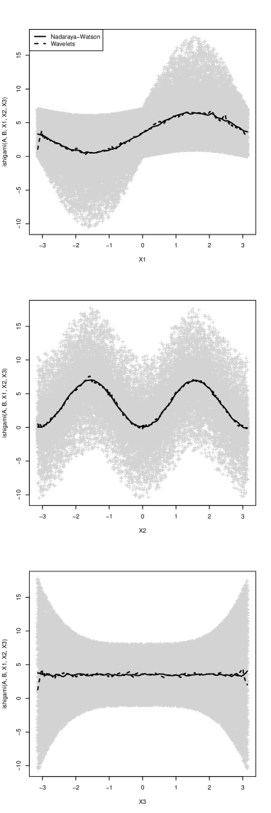
Figure 1: Example of regression obtained using Nadaraya-Watson and wavelets with $n(p+1)=40,000$ simulations for the Ishigami function. The conditional expectation of $Y$ knowing $X_{1}$ (resp. $X_{2}$ and $X_{3}$) is represented in line 1 (resp. 2 and 3).

Case 2

The results are presented in Table 2. As for Case 1, we see that in term of MSE, the non-parametric estimators overperform again the Jansen estimators. For $X_{1}$, the Nadaraya-Watson and wavelet estimators have comparable statistics, but the wavelet estimator is the best for $X_{2}$.

Table 2: Estimates of the bias and MSE for the parameters $X_{1}$ and $X_{2}$ in the Ishigmami function, when $X_{3}$ is considered as a pertubation parameter, for 1,000 replications and $n=10{,}000$

Method	$\mathbb{E}[\hat{S_{1}}-S_{1}]$	$\mathbb{E}[(\hat{S_{1}}-S_{1})^{2}]$	$\mathbb{E}[\hat{S_{2}}-S_{2}]$	$\mathbb{E}[(\hat{S_{2}}-S_{2})^{2}$
Jansen	$-$5,60E-04	2,00E-04	$-$7,80E-04	1,80E-04
Nadaraya-Watson	$-$1,80E-03	1,70E-05	$-$1,40E-02	2,00E-04
Wavelets	$-$7,00E-04	5,60E-05	1,90E-03	8,70E-05

Both non-parametric estimators depend on a tuning parameter: the window $h$ for Nadaraya-Watson and the constant $K$ for the wavelets. In Figure 2, the MSE are plotted as functions of the window $h$ (for the estimator with Nadaraya-Watson) and of the constant $K$ (for our estimator with wavelets). The performances of the wavelet estimator are much more stable with respect to the values of $K$ on the stochastic Ishigami model (Case 2).

Figure 2: MSE for the estimators using Nadaraya-Watson (dots) and wavelets (dash-dots) in the case of the stochastic Ishigami model (Case 2) for $n=10,000$: for $X_{1}$ (left) and $X_{2}$ (right). The MSE with Nadaraya-Watson estimators are plotted as functions of the window $h$ (bottom axis) and the MSE with wavelets are plotted as function of the constant $K$ (top axis).

To conclude these simulations on the stochastic Ishigami model, we plotted on logarithmic scales the MSE as function of the sample size $n$: see Figure 3. It is seen that the wavelet estimator is better than the Jansen estimator. For the wavelet estimator, the slope estimated with ordinary least squares equals to $-1.15$ for $X_{1}$ and $-1.12$ for $X_{2}$. This is in accordance with the value of $-$1 predicted by Corollary 2.6.

Figure 3: MSE for the Jansen estimators (plain), non-parametric estimator with Nadaraya-Watson (dots) and estimator with wavelets (dash-dots) in the case of the stochastic Ishigami model (Case 2) are represented as functions of $n$, which varies between $100$ and $10,000$. Left: for $X_{1}$. Right: for $X_{2}$. The graphs are plotted in logarithmic scales.

These results suggest that the proposed non-parametric estimator constitute an interesting alternative to the Jansen estimator, showing less variability and potentially requiring a lower number of simulations of the model, even in the deterministic setting of Case 1.

3 Sobol indices for epidemiological problems

We now consider two stochastic individual-based models of epidemiology in continuous time. In both cases, the population is of size $N$ and divided into compartments. Input parameters are the rates describing the times that individuals stay in each compartment. These rates are usually estimated from epidemiological studies or clinical trials, but there can be uncertainty on their values due to various reasons. The restricted size of the sample in these studies brings uncertainty on the estimates, which are given with uncertainty intervals (classically, a 95% confidence interval). Different studies can provide different estimates for the same parameters. The study populations can be subject to selection biases. In the case of clinical trials where the efficacy of a treatment is estimated, the estimates can be optimistic compared with what will be the effectiveness in real-life, due to the protocol of the trials. It is important to quantify how these uncertainties on the input parameters can impact the results and the conclusion of an epidemiological modelling study.

3.1 SIR model and ODE metamodels

In the first model, we consider the usual SIR model, with three compartments: susceptibles, infectious and removed (e.g. [1, 4, 11]). We denote by $S_{t}^{N}$, $I_{t}^{N}$ and $R_{t}^{N}$ the respective sizes of the corresponding sub-populations at time $t\geq 0$, with $S_{t}^{N}+I_{t}^{N}+R_{t}^{N}=N$. At the population level, infections occur at the rate $\frac{\lambda}{N}S_{t}^{N}I^{N}_{t}$ and removals at the rate $\mu I_{t}^{N}$. The idea is that to each pair of susceptible-infectious individuals a random independent clock with parameter $\lambda/N$ is attached and to each infectious individual an independent clock with parameter $\mu$ is attached.

The input parameters are the rates $\lambda$ and $\mu$. The outpout parameter is the final size of the epidemic, i.e. at a time $T>0$ where $I^{N}_{T}=0$, $Y=(I^{N}_{T}+R^{N}_{T})/N$.

It is possible to describe the evolution of $(S^{N}_{t}/N,I^{N}_{t}/N,R^{N}_{t}/N)_{t\geq 0}$ by a stochastic differential equation (SDE) driven by Poisson point measures (see e.g. [33]) and it is known that when $N\rightarrow+\infty$, this stochastic process converges in $\mathbb{D}(\mathbb{R}_{+},\mathbb{R}^{3})$ to the unique solution $(s_{t},i_{t},r_{t})_{t\geq 0}$ of the following system of ordinary differential equations (e.g. [1, 4, 11, 33]):

$$\left\{\begin{array}[]{l}\frac{ds}{dt}=-\lambda s_{t}i_{t}\\[3.0pt] \frac{di}{dt}=\lambda s_{t}i_{t}-\mu i_{t}\\[3.0pt] \frac{dr}{dt}=\mu i_{t}.\end{array}\right.$$ (3.1)

The fluctuations associated with this convergence have also been established. The limiting equations provide a natural deterministic approximating meta-model (recall [23]) for which sensitivity indices can be computed.

For the numerical experiment, we consider a close population of 1200 individuals, starting with $S_{0}^{1200}=1190$, $I_{0}^{1200}=10$ and $R_{0}^{1200}=0$. The parameters distributions are uniformly distributed with $\lambda/N\in[1/15000,3/15000]$ and $\mu\in[1/15,3/15]$. Here the randomness associated with the Poisson point measures is treated as the nuisance random factor in (1.2).

We compute the Jansen estimators of $S_{\lambda}$ and $S_{\mu}$ for the deterministic meta-model (3.1), with $n=30{,}000$ simulations ($n(p+1)=90{,}000$ calls to the function $f$) and choose these results as benchmark. For the estimators of $S_{\lambda}$ and $S_{\mu}$ in the SDE, we compute the Jansen estimators with $n=10{,}000$ (i.e. $n(p+1)=30{,}000$ calls to the function $f$), and the estimators based on Nadaraya-Watson and on wavelet regressions with $n=30{,}000$ simulations.

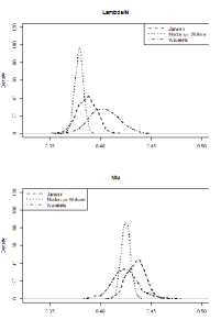
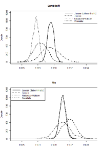
(a)	(b)

Figure 4: Estimations of the first order Sobol indices, using Jansen estimators on the meta-model with $n=10,000$ and the non-parametric estimations based on Nadaraya-Watson and wavelet regressions. (a): the distributions of the estimators of $S_{\lambda}$ and $S_{\mu}$ is approximated by Monte-carlo simulations. (b): the distributions of $\mathbb{E}(Y\ |\ \lambda)$ and $\mathbb{E}(Y\ |\ \mu)$ are approximated by Monte-Carlo simulations.

Let us comment on the results. The comparison of the different estimation methods is presented in Fig. 4. Since the variances in the meta-model and in the stochastic model differ, we start with comparing the distributions of $\mathbb{E}(Y\ |\ \lambda)$ and $\mathbb{E}(Y\ |\ \mu)$ that are centered around the same value, independently of whether the meta-model or the stochastic model is used (Fig. 4(b)). These distributions are obtained from 1,000 Monte-carlo simulations. Because theoretical values are not available, we take the meta-model as a benchmark. We see that the wavelet estimator performs well for both $\lambda$ and $\mu$ while Nadaraya-Watson regression estimator exhibit biases for $\lambda$. Jansen estimator on the stochastic model exhibit biases for both $\lambda$ and $\mu$.

We try to comment on the biases that are observed. When looking at Fig. 5, the simulations can give very noisy $Y$’s: extinctions of the epidemics can be seen in very short time in simulations, due to the initial randomness of the trajectories. This produces distributions for $Y$’s that are not unimodal or with peaks at 0, which makes the estimation of $\mathbb{E}(Y\ |\ \lambda)$ or $\mathbb{E}(Y\ |\ \mu)$ more difficult. The wavelet estimator seems to cope well with this situation.

In a second time, we focus on the estimation of the Sobol indices for the stochastic model with the SDE (we leave out the deterministic meta-model for the reasons mentioned above). The smoothed distributions of the estimators of $S_{\lambda}$ and $S_{\mu}$, for 1,000 Monte-Carlo replications, are presented in Fig. 4(a); the means and standard deviations of these distributions are given in Table 3. Although there is no theoretical values for $S_{\lambda}$ and $S_{\mu}$, we can see (Table 3) that the estimators of the Sobol indices with non-parametric regressions all give similar estimates in expectation for $\mu$. For $\lambda$, there are some discrepancies seen on Fig. 4(a) and Table 3.

Table 3: Estimators of the Sobol indices for $\lambda$ and $\mu$ and their standard deviations using $n=$10,000 Monte-Carlo replications of the stochastic SIR model.

	Jansen	Nadaraya-Watson	Wavelet
$\widehat{S}_{\lambda}$	0.39	0.38	0.40
s.d.	(9.2e-3)	(4.3e-3)	(1.4e-2)
$\widehat{S}_{\mu}$	0.44	0.42	0.42
s.d.	(9.0e-3)	(4.4e-3)	(1.2e-2)

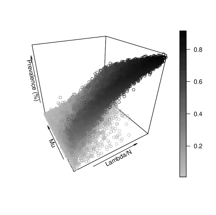
Figure 5: Prevalence ($Y$) simulated from the $n(p+1)=30,000$ simulations of $\lambda$ and $\mu$, for the SIR model.

3.2 Application to the spread of HVC among drug users

Chronic Hepatitis C virus (HCV) is a major cause of liver failure in the world, responsible of approximately 500,000 deaths annually [35]. HCV is a bloodborne disease, and the transmission remains high in people who inject drugs (PWID) due to injecting equipment sharing [32]. Until recently, the main approaches to decrease HCV transmission among PWID in high income countries relied on injection prevention and on risk reduction measures (access to sterile equipment, opioid substitution therapies, etc.). The arrival of highly effective antiviral treatments offers the opportunity to use the treatment as a mean to prevent HCV transmission, by treating infected PWID before they transmit the infection [13].

In this context, a stochastic, individual-based dynamic model was used to assess the impact of the treatment on HCV transmission in PWID in Paris area [8]. This model included HCV transmission on a random graph modelling PWID social network, the cascade of care of chronic hepatitis C and the progression of the liver disease. A brief description of the model for HCV infection and cascade of care is available in Fig. 6, for a detailed description and the values and uncertainty intervals of the parameters, the reader can refer to [8]. These parameters are the input of our model and we assume for them uniform distributions on their uncertainty intervals. Here, $Y$ is the prevalence after 10 years of simulation.

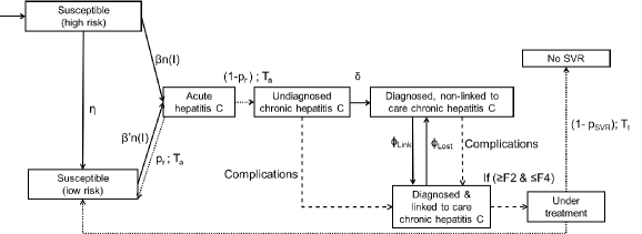
Figure 6: Diagram flow of infection and cascade of care modelling for HCV infection among PWID. Greek letters refer to rates, $p_{r}$ and $p_{SVR}$ to probabilities and $T_{a}$ and $T_{t}$ to (deterministic) time before leaving the compartment. $\beta$ depends on the status of the PWID with respect to the risk reduction measures (access to sterile injecting equipment, access to substitution therapies). $n_{i}$ denotes the number of infected injecting partners of the PWID. $\delta$ depends on the status of the PWID with respect to injection: active or inactive injector (i.e. before or after the cessation of injection). The liver disease progression is quantified by a score (score Metavir for the fibrosis progression) between F0 and F4 (cirrhosis). “Complications” refers to the two cirrhosis complications: decompensated cirrhosis and hepatocellular carcinoma

The parameter values used in this analysis were mainly provided by epidemiological studies and were subject to uncertainty. This kind of model requires high computing time, and thus the sensitivity analysis using Monte-Carlo estimators of Sobol indices is difficult, due to the number of simulations needed. Therefore, we focused on the seven main ones: infection rate per partner, transition rate F0/F1 $>$ F2/F3, rate of linkage to care and LFTU, average time to diagnosis, average time to cessation, relative risk of infection (1st year), mortality among active PWID. Other parameters contributions to the variance was considered as negligible and we considered these parameters as noise in our estimates.

We estimate Sobol indices using the wavelet non-parametric estimator. We used $n=10{,}000$ simulations of the model. We obtained unrealistic results using leave-one-out cross validation procedure to select the value of $K$ in the estimators proposed in 2.1. However, keeping values $\widehat{\beta}^{\ell}_{jk}$ with $j<3$ produce realistic estimates. Thus, we kept all these coefficients to produce the estimates.

For comparison, we also represented the sensitivity using a Tornado diagram, classically used in Epidemiology. To build the Tornado diagram, we first fix all the parameters but one to their values used in the analysis and we let the free parameter vary in an uncertainty interval. For each set of parameters thus obtained, the output $Y$ is computed. Then, the parameters are sorted by decreasing variations of $Y$, and the deviation from the main analysis results is represented in a bar plot. We can compare the orders of the input parameters given by the Sobol indices and by the Tornado diagram.

Figure 7: Tornado diagram (above): the variable $Y$ is plotted in abcissa and the vertical line corresponds to the expectation of $Y$ for the estimated parameters. We let each input variable vary separately between a lower bound and an upper bound, that are indicated left and right of each horizontal bar. The bars of the Tornado diagram are the corresponding values obtained for $Y$. Sobol indices (below): Sobol indices have been estimated using the wavelet estimators. Parameters have been sorted by decreasing values of their Sobol indices. What can be compared is the order of the various input variables in each method. LTFU=loss to follow-up, HCC=Hepatocellular carcinoma, M=Male, F=Female. “Cessation” refers to the cessation of the injections. “F0/F1 $>$ F2/F3” refers to the transition rate from a fibrosis score F0 or F1 to a fibrosis score F2 or F3 (and similarly for other rates).

The results are presented in Figure 7. Since the Sobol indices can be interpreted as the contribution of each parameter to the variance of $Y$, we can thus see that a large part of the variance of $Y$ is explained by the infection rate per infected partner alone, with a Sobol index of 0.6, and by the transition rate from a fibrosis score of F0/F1 to a score of F2/F3, with a Sobol index of 0.55. Next comes the linkage to care/loss to follow-up rate. The rankings of the input parameters obtained by the Sobol indices and the Tornado diagram (obtained in [8]) are in accordance for the main parameters. For the Tornado diagram, the most sensitive parameters (the infection rate per infected injecting partner, the transition rate from a fibrosis score of F0/F1 to a score of F2/F3 and the combination of the linkage to care/loss to follow-up rate) were also varied together to estimate the impact of the uncertainty about the linkage to care of PWID. The Tornado diagram, which explores a much smaller region of the parameter space by the way it is constructed, detects more noisy contributions for the other factors. This appears, in the Tornado, in the group of parameters having similar Sobol indices (average time to diagnosis and cessation, relative risk of infection, mortality, F2/F3$>$F4).

4 Conclusion

Sensitivity analysis is a key step in modelling studies, in particular in epidemiology. Models often have a high number of parameters, which are often seen as degrees of freedom to test scenarii and take into account several interplaying phenomena and factors. The computation of Sobol indices can indicate, among a long list of input parameters, which ones can have an important impact on the outputs. The classical estimators, like the Jansen estimator, require a large amount of requests to the function $f$ that generates the output from the inputs. The reason is that the Sobol indices are approximated, in these cases, by quantities involving imbricated sums where parameters vary one by one.

The literature on sensitivity analysis focuses on outputs that depend deterministically on the inputs. When there is randomness, it is natural to propose new approximations based on non-parametric estimations that require a lower number of calls to $f$ since information brought by simulations with close input parameters can also be used. No meta-model is requested. Numerical study on toy models show that these estimators can be used in deterministic settings too.

Independently and at the same time as us [7], Solís [29, 30] introduced an estimator of the Sobol indices of order 1 based on Nadaraya-Watson regressions. We hence focus in this paper on an estimator of the Sobol indices based on wavelet decompositions. For both of them, an elbow effect is proved: under sufficient regularities, convergence rates of order $1/\sqrt{n}$ can be achieved. On numerical toy examples, we obtained a better MSE with the wavelet estimators than with the Jansen estimator of same complexity. The non-parametric estimators allow a better exploration of the parameter space: for each simulation, the whole set of input parameters is drawn afresh. Compared with the Nadaraya-Watson estimator, the wavelet estimator is adaptative, which means that the unknown regularity of the model underlying the data does not need to be known to calibrate the estimator. On simulations, our estimator behaves similarly with Nadaraya-Watson estimator. When well-calibrated they can overcome some smoothing biases that can appear when the output is very noisy, which is the case in epidemic scenarii where there can be either large outbreaks or quick extinction due to stochasticity, for example.

Notice also that our proofs in the present paper are much shorter than the proofs needed to study the estimator based on Nadaraya-Watson regression. First, the wavelet estimator is a projection estimator and the difficulties related with the fact that there is a fraction in the Nadaraya-Watson estimator disappear. Second, we use elegant techniques (developed independently from sensitivity analysis) on empirical processes and concentration inequalities due to Castellan [5] to adapt the results of Laurent and Massard in the Gaussian case [21].

This first order index $S_{\ell}$ corresponds to the sensitivity of the model to $X_{\ell}$ alone. Higher order indices can also be defined using ANOVA decomposition: considering $(\ell,\ell^{\prime})\in\{1,\dots,p\}$, we can define the second order sensitivity, corresponding to the sensitivity of the model to the interaction between $X_{\ell}$ and $X_{\ell^{\prime}}$ index by

$$S_{\ell\ell^{\prime}}=\frac{\mbox{Var}\big{(}\mathbb{E}[Y\ |\ X_{\ell},X_{\ell^{\prime}}]\big{)}}{\mbox{Var}(Y)}-S_{\ell}-S_{\ell^{\prime}}$$ (4.1)

We can also define the total sensitivity indices by

$$S_{T_{\ell}}=\sum_{L\subset\{1,\dots,p\}\,|\,\ell\in L}S_{L}.$$ (4.2)

These indices allow to assess 1) the sensitivity of the model to each parameter taken separately and 2) the possible interactions, which are quantified by the difference between the total order and the first order index for each parameter. Estimation of higher order indices using non-parametric techniques would be an interesting subject for further researches.

5 Proofs

5.1 Proof of Theorem 2.4

We follow the scheme of the proof of Theorem 1 in [21]. The main difficulty here is that we are not in a Gaussian framework and that we use the empirical process $\bar{\gamma}_{n}$, which introduces much technical difficulties.

In the sequel, $C$ denotes a constant that can vary from line to line.

Using Lemma 2.2, we concentrate on the MSE $\mathbb{E}\big{(}(\widehat{V}_{\ell}-V_{\ell})^{2}\big{)}$. First, we will prove that:

$$\mathbb{E}\Big{[}\Big{(}\widehat{V}_{\ell}-V_{\ell}-\zeta_{n}\Big{)}^{2}\Big{]}\leq\inf_{\mathcal{J}\subset\{-1,\dots,J_{n}\}}\mathbb{E}\Big{[}\Big{(}-\widehat{V}_{\mathcal{J},\ell}+\mbox{pen}(\mathcal{J})+V_{\ell}+\zeta_{n}\Big{)}^{2}_{+}\Big{]}+\frac{C\log_{2}^{2}(n)}{n^{3/2}},$$ (5.1)

where $\widehat{V}_{\mathcal{J},\ell}$ has been defined in (2.16). The penalization term associated to a subset $\mathcal{J}\subset\{-1,\dots J_{n}\}$ has been defined in (2.9). Then, considering the first term in the r.h.s. of (5.1), we prove:

$$\mathbb{E}\Big{[}\Big{(}-\widehat{V}_{\mathcal{J},\ell}+\mbox{pen}(\mathcal{J})+V_{\ell}+\zeta_{n}\Big{)}^{2}_{+}\Big{]}\leq C\Big{(}\|h_{\ell}-h_{\mathcal{J},\ell}\|_{2}^{4}+\frac{\mbox{Card}^{2}(\mathcal{J})}{n^{2}}\Big{)}$$ (5.2)

Step 1:

From (2.10), and letting $A_{\mathcal{J}}=\widehat{V}_{\mathcal{J},\ell}-\mbox{pen}(\mathcal{J})-V_{\ell}-\zeta_{n}$, we have:

$$\widehat{V}_{\ell}-V_{\ell}-\zeta_{n}=\sup_{\mathcal{J}\subset\{-1,\dots,J_{n}\}}A_{\mathcal{J}}.$$

Since

$$\sup_{\mathcal{J}}A_{\mathcal{J}}=\sup_{\mathcal{J}}\big{(}A_{\mathcal{J}}\big{)}_{+}\ {\mathchoice{\rm 1\mskip-4.0mul}{\rm 1\mskip-4.0mul}{\rm 1\mskip-4.5mul}{\rm 1\mskip-5.0mul}}_{\{\sup_{\mathcal{J}}A_{\mathcal{J}}\geq 0\}}-\inf_{\mathcal{J}}\big{(}A_{\mathcal{J}}\big{)}_{-}\ {\mathchoice{\rm 1\mskip-4.0mul}{\rm 1\mskip-4.0mul}{\rm 1\mskip-4.5mul}{\rm 1\mskip-5.0mul}}_{\{\sup_{\mathcal{J}}A_{\mathcal{J}}<0\}},$$

we obtain by taking the absolute values that

$$\Big{|}\sup_{\mathcal{J}}A_{\mathcal{J}}\Big{|}\leq\max\Big{[}\sup_{\mathcal{J}}\big{(}A_{\mathcal{J}}\big{)}_{+},\inf_{\mathcal{J}}\big{(}A_{\mathcal{J}}\big{)}_{-}\Big{]}.$$

This provides that

$$\mathbb{E}\Big{(}\sup_{\mathcal{J}}A^{2}_{\mathcal{J}}\Big{)}\leq \sum_{\mathcal{J}\subset\{-1,\dots,J_{n}\}}\mathbb{E}\Big{(}\big{(}A_{\mathcal{J}}\big{)}^{2}_{+}\Big{)}+\inf_{\mathcal{J}\subset\{-1,\dots,J_{n}\}}\mathbb{E}\Big{(}\big{(}A_{\mathcal{J}}\big{)}^{2}_{-}\Big{)}$$

$$\leq \sum_{\mathcal{J}\subset\{-1,\dots,J_{n}\}}\mathbb{E}\Big{(}\big{(}A_{\mathcal{J}}\big{)}^{2}_{+}\Big{)}+\inf_{\mathcal{J}\subset\{-1,\dots,J_{n}\}}\mathbb{E}\Big{(}\big{(}-\widehat{V}_{\mathcal{J},\ell}+\mbox{pen}(\mathcal{J})+V_{\ell}+\zeta_{n}\big{)}^{2}_{+}\Big{)}.$$ (5.3)

The second term corresponds to what appears in (5.1) and will be treated in Step 4 to obtain (5.2). Let us consider the first term of the r.h.s.

From (2.9), we have:

$$\mbox{pen}(\mathcal{J})= \sum_{j\in\mathcal{J}}w(j)=\frac{K}{n}\sum_{j\in\mathcal{J}}(2^{j}+\log 2)=\mbox{pen}_{1}(\mathcal{J})+\mbox{pen}_{2}(\mathcal{J}),$$ (5.4)

with

$$\mbox{pen}_{1}(\mathcal{J})= \frac{K}{n}\sum_{j\in\mathcal{J}}2^{j}$$ (5.5)

$$\mbox{pen}_{2}(\mathcal{J})= \mbox{pen}(\mathcal{J})-\mbox{pen}_{1}(\mathcal{J})=\frac{K}{n}\mbox{Card}(\mathcal{J})\ \log 2.$$ (5.6)

Using this, we start by rewriting

$$A_{\mathcal{J}}= \widehat{V}_{\mathcal{J},\ell}-\mbox{pen}(\mathcal{J})-V_{\ell}-\zeta_{n}$$

$$= \|\widehat{h}_{\mathcal{J},\ell}\|^{2}_{2}-\mbox{pen}(\mathcal{J})-\|h_{\ell}\|^{2}_{2}-\zeta_{n}$$

$$= \big{(}\|\widehat{h}_{\mathcal{J},\ell}-h_{\mathcal{J},\ell}\|^{2}_{2}+\|h_{\mathcal{J},\ell}\|^{2}_{2}+2\langle\widehat{h}_{\mathcal{J},\ell}-h_{\mathcal{J},\ell},h_{\mathcal{J},\ell}\rangle\big{)}$$

$$-\big{(}\|h_{\ell}-h_{\mathcal{J},\ell}\|^{2}_{2}+\|h_{\mathcal{J},\ell}\|^{2}_{2}+2\langle h_{\ell}-h_{\mathcal{J},\ell},h_{\mathcal{J},\ell}\rangle\big{)}-\zeta_{n}-\mbox{pen}(\mathcal{J})$$

$$= \|\widehat{h}_{\mathcal{J},\ell}-h_{\mathcal{J},\ell}\|^{2}_{2}-\mbox{pen}_{1}(\mathcal{J})+2\langle\widehat{h}_{\mathcal{J},\ell}-h_{\mathcal{J},\ell},h_{\mathcal{J},\ell}\rangle-\|h_{\ell}-h_{\mathcal{J},\ell}\|^{2}_{2}-\zeta_{n}-\mbox{pen}_{2}(\mathcal{J}),$$ (5.7)

since $\langle h_{\ell}-h_{\mathcal{J},\ell},h_{\mathcal{J},\ell}\rangle=0$ by definition of $h_{\mathcal{J},\ell}$ as projection of $h_{\ell}$ on the subspace generated by $\{\psi_{jk},\ j\in\mathcal{J},\,k\in\mathbb{Z}\}$.

Thus:

$$\mathbb{E}\Big{(}\big{(}A_{\mathcal{J}}\big{)}^{2}_{+}\Big{)}\leq 2\mathbb{E}\Big{(}\big{(}\|\widehat{h}_{\mathcal{J},\ell}-h_{\mathcal{J},\ell}\|^{2}_{2}-\mbox{pen}_{1}(\mathcal{J})\big{)}^{2}\Big{)}\\ +2\mathbb{E}\Big{(}\big{(}2\langle\widehat{h}_{\mathcal{J},\ell}-h_{\mathcal{J},\ell},h_{\mathcal{J},\ell}\rangle-\|h_{\ell}-h_{\mathcal{J},\ell}\|^{2}_{2}-\zeta_{n}-\mbox{pen}_{2}(\mathcal{J})\big{)}^{2}\Big{)}.$$ (5.8)

The first term in the r.h.s. is treated in Step 2, and the second term in Step 3. After summation over $\mathcal{J}\subset\{-1,\dots,J_{n}\}$, this provides an upper bound for the first term in the r.h.s. of (5.3) which provides (5.1).

Step 2: Upper bound of the first term in the r.h.s. of (5.8)

Reformulation of $\|\widehat{h}_{\mathcal{J},\ell}-h_{\mathcal{J},\ell}\|^{2}_{2}$

The first term in the r.h.s. of (5.7) is the approximation error of $h_{\mathcal{J}}$ by $\widehat{h}_{\mathcal{J},\ell}$ and equals

$$\|\widehat{h}_{\mathcal{J},\ell}-h_{\mathcal{J},\ell}\|^{2}_{2}=\sum_{j\in\mathcal{J}}\sum_{k\in\mathbb{Z}}\big{(}\widehat{\beta}_{jk}-\beta_{jk}\big{)}^{2}=\sum_{j\in\mathcal{J}}\sum_{k\in\mathbb{Z}}\bar{\gamma}_{n}\big{(}\psi_{jk}\big{)}^{2}.$$

To control it, let us introduce, for coefficients $a=(a_{jk},\ -1\leq j\leq J_{n},\ k\in\mathbb{Z})$, the set

$$\mathcal{F}_{1,\mathcal{J}}=\Big{\{}f=\sum_{j\in\mathcal{J}}\sum_{k\in\mathbb{Z}}a_{jk}\psi_{jk},\ a_{jk}\in\mathbb{Q},\ \|a\|_{2}\leq 1\Big{\}},$$

which is countable and dense in the unit ball of $L^{2}([0,1])$. Thus,

$$\Big{(}\sum_{j\in\mathcal{J}}\sum_{k\in\mathbb{Z}}\bar{\gamma}_{n}\big{(}\psi_{jk}\big{)}^{2}\Big{)}^{1/2}= \sup_{\|a\|_{2}\leq 1}\Big{|}\sum_{j\in\mathcal{J}}\sum_{k\in\mathbb{Z}}a_{jk}\bar{\gamma}_{n}\big{(}\psi_{jk}\big{)}\Big{|}$$

$$= \sup_{\|a\|_{2}\leq 1}\Big{|}\bar{\gamma}_{n}\Big{(}\sum_{j\in\mathcal{J}}\sum_{k\in\mathbb{Z}}a_{jk}\psi_{jk}\Big{)}\Big{|}$$

$$= \sup_{f\in\mathcal{F}_{1,\mathcal{J}}}\big{|}\bar{\gamma}_{n}(f)\big{|}:=\chi_{n}(\mathcal{J}).$$ (5.9)

Let us introduce, for $\rho>0$,

$$\Omega_{\mathcal{J}}(\rho)=\big{\{}\forall j\in\mathcal{J},\,\sum_{k\in\mathbb{Z}}\big{|}\bar{\gamma}_{n}(\psi_{jk})\big{|}\leq\rho 2^{-j/2}\big{\}}.$$ (5.10)

Then, to upper bound the first term in (5.8), we can write:

$$\mathbb{E}\Big{(}\big{(}\|\widehat{h}_{\mathcal{J},\ell}-h_{\mathcal{J},\ell}\|^{2}_{2}-\mbox{pen}_{1}(\mathcal{J})\big{)}^{2}\Big{)}\leq 2A_{1}(\mathcal{J})+2A_{2}(\mathcal{J})$$ (5.11)

where, for $\chi_{n}(\mathcal{J})$ defined in (5.9),

$$A_{1}(\mathcal{J})=\mathbb{E}\Big{(}\big{(}\chi_{n}^{2}(\mathcal{J}){\mathchoice{\rm 1\mskip-4.0mul}{\rm 1\mskip-4.0mul}{\rm 1\mskip-4.5mul}{\rm 1\mskip-5.0mul}}_{\Omega_{\mathcal{J}}(\rho)}-\mbox{pen}_{1}(\mathcal{J})\big{)}^{2}\Big{)},$$

and $$A_{2}(\mathcal{J})=\mathbb{E}\Big{(}\chi_{n}^{4}(\mathcal{J}){\mathchoice{\rm 1\mskip-4.0mul}{\rm 1\mskip-4.0mul}{\rm 1\mskip-4.5mul}{\rm 1\mskip-5.0mul}}_{\Omega^{c}_{\mathcal{J}}(\rho)}\Big{)}.$$ (5.12)

The upper bounds of $A_{1}(\mathcal{J})$ and $A_{2}(\mathcal{J})$ make the object of the remainder of Step 2. We use ideas developed in [5].

Upper bound for $A_{1}(\mathcal{J})$

To upper bound $A_{1}(\mathcal{J})$, we use the identity

$$A_{1}(\mathcal{J})=\int_{0}^{+\infty}2t\ \mathbb{P}\big{(}\chi_{n}^{2}(\mathcal{J}){\mathchoice{\rm 1\mskip-4.0mul}{\rm 1\mskip-4.0mul}{\rm 1\mskip-4.5mul}{\rm 1\mskip-5.0mul}}_{\Omega_{\mathcal{J}}(\rho)}-\mbox{pen}_{1}(\mathcal{J})>t\big{)}\ dt,$$ (5.13)

and look for deviation inequalities of $\chi_{n}^{2}(\mathcal{J}){\mathchoice{\rm 1\mskip-4.0mul}{\rm 1\mskip-4.0mul}{\rm 1\mskip-4.5mul}{\rm 1\mskip-5.0mul}}_{\Omega_{\mathcal{J}}(\rho)}$. Then, estimates of the probability of $\Omega^{c}_{\mathcal{J}}(\rho)$ are studied to control $A_{2}(\mathcal{J})$.

Recall that $\chi_{n}(\mathcal{J})$ (resp. $\Omega_{\mathcal{J}}(\rho)$) has been defined in (5.9) (resp. (5.10)). The supremum in (5.9) is obtained for

$$\bar{a}_{jk}=\frac{\bar{\gamma}_{n}(\psi_{jk})}{\chi_{n}(\mathcal{J})}.$$ (5.14)

On the set $\Omega_{\mathcal{J}}(\rho)\cap\{\chi_{n}(\mathcal{J})>z\}$, for a constant $z>0$ that shall be fixed in the sequel, we have for all $j\in\mathcal{J}$,

$$\sum_{k\in\mathbb{Z}}\big{|}\bar{a}_{jk}\big{|}=\frac{\sum_{k\in\mathbb{Z}}\big{|}\bar{\gamma}_{n}(\psi_{jk})\big{|}}{\chi_{n}(\mathcal{J})}\leq\frac{\rho 2^{-j/2}}{z}.$$

As a consequence, on the set $\Omega_{\mathcal{J}}(\rho)\cap\{\chi_{n}(\mathcal{J})>z\}$, we can restrict the research of the optima to the set

$$\Lambda_{\mathcal{J}}=\Big{\{}f=\sum_{j\in\mathcal{J}}\sum_{k\in\mathbb{Z}}a_{jk}\psi_{jk}\in\mathcal{F}_{1,\mathcal{J}},\\ \mbox{ and }\ a_{jk}=0\mbox{ if }j\notin\mathcal{J},\ \sum_{k\in\mathbb{Z}}\big{|}a_{jk}\big{|}\leq\frac{\rho 2^{-j/2}}{z}\mbox{ if }j\in\mathcal{J}\Big{\}},$$ (5.15)

which is countable.

We can then use Talagrand inequality (see [24, p.170]) to obtain that for all $\eta>0$ and $x>0$,

$$\mathbb{P}\Big{(}\sup_{f\in\Lambda_{\mathcal{J}}}\big{|}\bar{\gamma}_{n}(f)\big{|}\geq(1+\eta)\mathbb{E}\big{(}\sup_{f\in\Lambda_{\mathcal{J}}}\big{|}\bar{\gamma}_{n}(f)\big{|}\big{)}+\sqrt{2\nu_{n}x}+\big{(}\frac{1}{3}+\frac{1}{\eta}\big{)}b_{n}x\Big{)}\leq e^{-x},$$ (5.16)

where the quantities $\nu_{n}$ and $b_{n}$ can be chosen respectively as $\nu_{n}=M^{2}/n$ and $b_{n}=2M\|\psi\|_{\infty}\rho\mbox{Card}(\mathcal{J})/nz$.

Indeed, $\nu_{n}$ is an upper bound of:

$$\frac{1}{n}\sup_{f\in\Lambda_{\mathcal{J}}}\mbox{Var}\Big{(}Y_{1}f\big{(}G_{\ell}(X_{\ell}^{1})\big{)}\Big{)}\leq\frac{M^{2}}{n}\sup_{f\in\Lambda_{\mathcal{J}}}\|f\|_{2}^{2}\leq\frac{M^{2}}{n},$$ (5.17)

where the last inequality comes from the definition of $\Lambda_{\mathcal{J}}$ and $\mathcal{F}_{1,\mathcal{J}}$.

As for the term $b_{n}$, it is an upper bound of:

$$\frac{1}{n}\sup_{f\in\Lambda_{\mathcal{J}}}\sup_{(u,y)\in[0,1]\times[-M,M]}\Big{|}yf(u)-\mathbb{E}\Big{(}Y_{1}f\big{(}G_{\ell}(X_{\ell}^{1})\big{)}\Big{)}\Big{|}\\ \leq\frac{2M}{n}\sum_{j\in\mathcal{J}}\sum_{k\in\mathbb{Z}}|a_{jk}|2^{j/2}\|\psi\|_{\infty}\leq\frac{2M\|\psi\|_{\infty}}{n}\sum_{j\in\mathcal{J}}\frac{\rho 2^{-j/2}}{z}2^{j/2}=\frac{2M\|\psi\|_{\infty}\rho\ \mbox{Card}(\mathcal{J})}{n\ z},$$ (5.18)

if $f=\sum_{j\in\mathcal{J}}\sum_{k\in\mathbb{Z}}a_{jk}\psi_{jk}$. For the expectation appearing in the probability in the r.h.s. of (5.16), we have:

$$\mathbb{E}\big{(}\sup_{f\in\Lambda_{\mathcal{J}}}\big{|}\bar{\gamma}_{n}(f)\big{|}\big{)}\leq\mathbb{E}\big{(}\chi_{n}(\mathcal{J})\big{)}\leq\sqrt{\mathbb{E}\big{(}\chi_{n}^{2}(\mathcal{J})\big{)}}=\sqrt{\sum_{j\in\mathcal{J}}\sum_{k\in\mathbb{Z}}\mathbb{E}\big{(}\bar{\gamma}_{n}^{2}(\psi_{jk})\big{)}}$$

$$\hskip 79.6678pt=\sqrt{\sum_{j\in\mathcal{J}}\sum_{k\in\mathbb{Z}}\frac{1}{n}\mbox{Var}\big{(}Y_{1}\psi_{jk}(G_{\ell}(X^{1}_{\ell}))\big{)}}$$

$$\hskip 79.6678pt\leq\sqrt{\sum_{j\in\mathcal{J}}\sum_{k\in\mathbb{Z}}\frac{1}{n}\mathbb{E}\big{(}Y_{1}^{2}\psi^{2}_{jk}(G_{\ell}(X^{1}_{\ell}))\big{)}}$$

$$\hskip 79.6678pt\leq\frac{M}{\sqrt{n}}\sqrt{\sum_{j\in\mathcal{J}}\sum_{k\in\mathbb{Z}}\int_{0}^{1}\psi^{2}_{jk}(u)du}\leq\frac{M}{\sqrt{n}}\sqrt{C^{\prime}\sum_{j\in\mathcal{J}}2^{j}}$$ (5.19)

by the fact that the wavelets $\psi_{jk}$ have compact supports and satisfy $\|\psi_{jk}\|_{2}^{2}=1$. The constant $C^{\prime}$ in (5.19) is the number of wavelets $(\psi_{0k})_{k\in\mathbb{Z}}$ that intersect $[0,1]$. Thus for a given $j\geq 0$, the number of wavelets $(\psi_{jk})_{k\in\mathbb{Z}}$ that instersect $[0,1]$ is of order $2^{j}C^{\prime}$.

Because we have on $\Omega_{\mathcal{J}}(\rho)\cap\{\chi_{n}(\mathcal{J})>z\}$ that $\chi_{n}(\mathcal{J})=\sup_{f\in A_{\mathcal{J}}}\big{|}\bar{\gamma}_{n}(f)\big{|}$, we deduce that $\sup_{f\in A_{\mathcal{J}}}\big{|}\bar{\gamma}_{n}(f)\big{|}\geq\chi_{n}(\mathcal{J}){\mathchoice{\rm 1\mskip-4.0mul}{\rm 1\mskip-4.0mul}{\rm 1\mskip-4.5mul}{\rm 1\mskip-5.0mul}}_{\Omega_{\mathcal{J}}(\rho)\cap\{\chi_{n}(\mathcal{J}>z\}}$. Then, Equations (5.16)-(5.19) become:

$$\mathbb{P}\Big{(}\chi_{n}(\mathcal{J}){\mathchoice{\rm 1\mskip-4.0mul}{\rm 1\mskip-4.0mul}{\rm 1\mskip-4.5mul}{\rm 1\mskip-5.0mul}}_{\Omega_{\mathcal{J}}(\rho)\cap\{\chi_{n}(\mathcal{J})>z\}}\geq(1+\eta)M\sqrt{\frac{C^{\prime}\sum_{j\in\mathcal{J}}2^{j}}{n}}+\sqrt{\frac{2M^{2}x}{n}}\\ +\big{(}\frac{1}{3}+\frac{1}{\eta}\big{)}\frac{2M\|\psi\|_{\infty}\rho\ \mbox{Card}(\mathcal{J})}{n\ z}x\Big{)}\leq e^{-x}.$$

Choosing $z=\sqrt{\frac{2x}{n}}\big{(}\frac{1}{3}+\frac{1}{\eta}\big{)}\|\psi\|_{\infty}$, we obtain:

$$\mathbb{P}\Big{(}\chi_{n}(\mathcal{J}){\mathchoice{\rm 1\mskip-4.0mul}{\rm 1\mskip-4.0mul}{\rm 1\mskip-4.5mul}{\rm 1\mskip-5.0mul}}_{\Omega_{\mathcal{J}}(\rho)\cap\{\chi_{n}(\mathcal{J})>z\}}\geq(1+\eta)M\sqrt{\frac{C^{\prime}\sum_{j\in\mathcal{J}}2^{j}}{n}}+(1+\rho\mbox{Card}(\mathcal{J}))M\sqrt{\frac{2x}{n}}\Big{)}\leq e^{-x}.$$

For the choice of $\rho=\big{(}\frac{1}{3}+\frac{1}{\eta}\big{)}\|\psi\|_{\infty}$, the r.h.s. in the probability above is larger than $z=\sqrt{\frac{2x}{n}}\big{(}\frac{1}{3}+\frac{1}{\eta}\big{)}\|\psi\|_{\infty}$, and we can get rid of the constraint $\{\chi_{n}(\mathcal{J})>z\}$. Finally, choosing $x=x_{\mathcal{J}}+\xi$, with

$$x_{\mathcal{J}}=\log\Big{(}\sum_{j\in\mathcal{J}}2^{j}\Big{)},$$ (5.20)

we obtain by using $(a+b)^{2}\leq 2a^{2}+2b^{2}$ that:

$$\mathbb{P}\Big{(}\chi^{2}_{n}(\mathcal{J}){\mathchoice{\rm 1\mskip-4.0mul}{\rm 1\mskip-4.0mul}{\rm 1\mskip-4.5mul}{\rm 1\mskip-5.0mul}}_{\Omega_{\mathcal{J}}(\rho)}-\frac{2}{n}\Big{[}(1+\eta)^{2}M^{2}C^{\prime}\sum_{j\in\mathcal{J}}2^{j}+2(1+\rho\mbox{Card}(\mathcal{J}))^{2}M^{2}x_{\mathcal{J}}\Big{]}\geq h_{\mathcal{J}}(\xi)\Big{)}\\ \leq e^{-x_{\mathcal{J}}}e^{-\xi},$$

where

$$h_{\mathcal{J}}(\xi)=\frac{4(1+\rho\mbox{Card}(\mathcal{J}))^{2}M^{2}}{n}\xi.$$ (5.21)

The square bracket in the l.h.s. inside the probability can be upper bounded by $n\mbox{pen}_{1}(\mathcal{J})=K\sum_{j\in\mathcal{J}}2^{j}$, for an appropriate constant $K$ that does not depend on $\mathcal{J}$. Indeed, denoting by $J_{\mbox{{\scriptsize max}}}=\max\mathcal{J}$, we have that $\mbox{Card}^{2}(\mathcal{J})\leq J_{\mbox{{\scriptsize max}}}^{2}$ while $\sum_{j\in\mathcal{J}}2^{j}\geq 2^{J_{\mbox{{\scriptsize max}}}}$. Since $2^{j}\geq j^{2}$ for all interger $j\not=3$, the result follows. Then:

$$\mathbb{P}\Big{(}\chi^{2}_{n}(\mathcal{J}){\mathchoice{\rm 1\mskip-4.0mul}{\rm 1\mskip-4.0mul}{\rm 1\mskip-4.5mul}{\rm 1\mskip-5.0mul}}_{\Omega_{\mathcal{J}}(\rho)}-\mbox{pen}_{1}\big{(}\mathcal{J}\big{)}\geq h_{\mathcal{J}}(\xi)\Big{)}\leq e^{-x_{\mathcal{J}}}e^{-\xi}.$$ (5.22)

From (5.13) and (5.22),

$$A_{1}(\mathcal{J})\leq\int_{0}^{+\infty}2te^{-x_{\mathcal{J}}}e^{-h_{\mathcal{J}}^{-1}(t)}dt,$$

with

$$h_{\mathcal{J}}^{-1}(t)=\frac{nt}{4(1+\rho\mbox{Card}(\mathcal{J}))^{2}M^{2}}.$$

Thus:

$$A_{1}(\mathcal{J})\leq \int_{0}^{+\infty}2te^{-x_{\mathcal{J}}}\exp\Big{(}-\frac{nt}{4(1+\rho\mbox{Card}(\mathcal{J}))^{2}M^{2}}\Big{)}dt$$

$$\leq \frac{32(1+\rho\mbox{Card}(\mathcal{J}))^{4}M^{4}}{n^{2}}e^{-x_{\mathcal{J}}}\leq C\frac{\mbox{Card}^{4}(\mathcal{J})e^{-x_{\mathcal{J}}}}{n^{2}}$$

$$\leq \frac{C\mbox{Card}^{2}(\mathcal{J})}{n^{2}},$$ (5.23)

using $(\sum_{j\in\mathcal{J}}2^{j})^{-1}\leq C/\mbox{Card}^{2}(\mathcal{J})$.

From the choice of $x_{\mathcal{J}}$ (5.20), we have:

$$\sum_{\mathcal{J}\subset\{-1,\dots,J_{n}\}}\mbox{Card}^{2}(\mathcal{J})\leq C2^{J_{n}}J_{n}^{2}\leq C\sqrt{n}\log_{2}^{2}(n),$$

by choice of $J_{n}=\log_{2}\big{(}\sqrt{n}\big{)}$. From this and (5.23), we deduce that:

$$\sum_{\mathcal{J}\subset\{-1,\dots,J_{n}\}}A_{1}(\mathcal{J})\leq\frac{C\log_{2}^{2}(n)}{n^{3/2}}.$$ (5.24)

Upper bound of $A_{2}(\mathcal{J})$

For the term $A_{2}(\mathcal{J})$ of (5.11), we have, for $(j,k)$ such that $j\not=-1$:

$$|\bar{\gamma}_{n}(\psi_{jk})|\leq M2^{j/2}\|\psi\|_{\infty}+M2^{-j/2}\int_{\mathbb{R}}|\psi(u)|du.$$

Thus, for a constant $C$ that depends only on the choice of $\psi_{-10}$ and $\psi_{00}$:

$$A_{2}(\mathcal{J})\leq\Big{[}C\sum_{j\in\mathcal{J}}\Big{(}M2^{j/2}\|\psi\|_{\infty}+M2^{-j/2}\int_{\mathbb{R}}|\psi(u)|du\Big{)}^{2}\Big{]}^{2}\times\mathbb{P}\Big{(}\Omega^{c}_{\mathcal{J}}(\rho)\Big{)}.$$ (5.25)

Since:

$$\sum_{i=1}^{n}\mathbb{E}\Big{[}\Big{(}\frac{Y_{i}\psi_{jk}\big{(}G_{\ell}(X_{\ell}^{i})\big{)}-\mathbb{E}\big{(}Y_{1}\psi_{jk}(G_{\ell}(X_{\ell}^{1}))\big{)}}{n}\Big{)}^{2}\Big{]}=\frac{\mbox{Var}\big{(}Y_{1}\psi_{jk}(G_{\ell}(X_{\ell}^{1}))\big{)}}{n}\leq\frac{M^{2}}{n},$$

$$\Big{|}\frac{Y_{i}\psi_{jk}\big{(}G_{\ell}(X_{\ell}^{i})\big{)}-\mathbb{E}\big{(}Y_{1}\psi_{jk}(G_{\ell}(X_{\ell}^{1}))\big{)}}{n}\Big{|}\leq\frac{2M2^{j/2}\|\psi\|_{\infty}}{n}\mbox{ a.s.}$$

then we have by Bernstein’s inequality (e.g. [24]):

$$\mathbb{P}\big{(}\big{|}\bar{\gamma}_{n}(\psi_{jk})\big{|}\geq\rho 2^{-j/2}\big{)}\leq 2\exp\Big{(}-\frac{n\rho^{2}2^{-j}}{2\big{(}M^{2}+2M\|\psi\|_{\infty}\rho\big{)}}\Big{)}.$$

As a consequence, recalling that $J_{\mbox{{\scriptsize max}}}=\max\mathcal{J}$, we have

$$\sum_{\mathcal{J}\subset\{-1,\dots J_{n}\}}A_{2}(\mathcal{J})\leq \sum_{\mathcal{J}\subset\{-1,\dots J_{n}\}}2^{2J_{\mbox{{\scriptsize max}}}}\mathbb{P}\Big{(}\exists(j,k)\in\mathcal{J}\times\mathbb{Z},\ \big{|}\bar{\gamma}_{n}(\psi_{jk})\big{|}\geq\rho 2^{-j/2}\Big{)}$$

$$\leq C\sum_{\mathcal{J}\subset\{-1,\dots J_{n}\}}2^{3J_{\mbox{{\scriptsize max}}}}\exp\Big{(}-\frac{n\rho^{2}2^{-J_{\mbox{{\scriptsize max}}}}}{2\big{(}M^{2}+2M\|\psi\|_{\infty}\rho\big{)}}\Big{)},$$ (5.26)

which is smaller than $C/n^{3/2}$ for sufficiently large $n$, as $J_{\mbox{{\scriptsize max}}}\leq J_{n}=\log_{2}(\sqrt{n})$.

Step 3: Upper bound of the second term in the r.h.s. of (5.8)

For the second term in the r.h.s. of (5.8),

$$2\langle\widehat{h}_{\mathcal{J},\ell}-h_{\mathcal{J},\ell},h_{\mathcal{J},\ell}\rangle-\|h_{\ell}-h_{\mathcal{J},\ell}\|^{2}_{2}-\zeta_{n}-\mbox{pen}_{2}(\mathcal{J})$$

$$= 2\sum_{j\in\mathcal{J}}\sum_{k\in\mathbb{Z}}\bar{\gamma}_{n}\big{(}\psi_{jk}\big{)}\beta_{jk}^{\ell}-\|h_{\ell}-h_{\mathcal{J},\ell}\|^{2}_{2}-2\bar{\gamma}_{n}\big{(}h_{\ell}\big{)}-\mbox{pen}_{2}(\mathcal{J})$$

$$= 2\bar{\gamma}_{n}\Big{(}\sum_{j\in\mathcal{J}}\sum_{k\in\mathbb{Z}}\beta_{jk}^{\ell}\psi_{jk}\Big{)}-\|h_{\ell}-h_{\mathcal{J},\ell}\|^{2}_{2}-2\bar{\gamma}_{n}\big{(}h_{\ell}\big{)}-\mbox{pen}_{2}(\mathcal{J})$$

$$= 2\bar{\gamma}_{n}\big{(}h_{\mathcal{J},\ell}-h_{\ell}\big{)}-\|h_{\ell}-h_{\mathcal{J},\ell}\|^{2}_{2}-\mbox{pen}_{2}(\mathcal{J})$$ (5.27)

$$\leq \Big{(}\frac{\bar{\gamma}_{n}\big{(}h_{\mathcal{J},\ell}-h_{\ell}\big{)}}{\|h_{\ell}-h_{\mathcal{J},\ell}\|_{2}}\Big{)}^{2}-\mbox{pen}_{2}(\mathcal{J})=\bar{\gamma}_{n}^{2}\Big{(}\frac{h_{\mathcal{J},\ell}-h_{\ell}}{\|h_{\ell}-h_{\mathcal{J},\ell}\|_{2}}\Big{)}-\mbox{pen}_{2}(\mathcal{J}),$$ (5.28)

by using the identity $2ab-b^{2}\leq a^{2}$. Setting $\varphi_{\mathcal{J}}=\frac{h_{\mathcal{J},\ell}-h_{\ell}}{\|h_{\ell}-h_{\mathcal{J},\ell}\|_{2}}$ and using Bernstein’s formula (see [24, p.25]), we have for all $x>0$:

$$\mathbb{P}\Big{(}\bar{\gamma}_{n}\big{(}\varphi_{\mathcal{J}}\big{)}\geq\sqrt{\frac{2M^{2}}{n}x}+\frac{2M\|\varphi_{\mathcal{J}}\|_{\infty}}{n}x\Big{)}\leq e^{-x}.$$ (5.29)

Setting $x=x_{\mathcal{J}}+\xi$ with now

$$x_{\mathcal{J}}=\mbox{Card}(\mathcal{J})\log 2,$$ (5.30)

and using that $(a+b)^{2}\leq 2a^{2}+2b^{2}$, we obtain that

$$\mathbb{P}\Big{(}\bar{\gamma}^{2}_{n}\big{(}\varphi_{\mathcal{J}}\big{)}-\Big{[}\frac{4M^{2}}{n}x_{\mathcal{J}}+\frac{16M^{2}\|\varphi_{\mathcal{J}}\|_{\infty}^{2}}{n^{2}}x_{\mathcal{J}}^{2}\Big{]}\geq r_{n}(\xi)\Big{)}\leq e^{-x_{\mathcal{J}}}e^{-\xi},$$ (5.31)

where and

$$r_{n}(\xi)=\frac{16M^{2}\|\varphi_{\mathcal{J}}\|_{\infty}^{2}\xi^{2}}{n^{2}}+\frac{4M^{2}\xi}{n}.$$

Let us consider the square bracket in (5.31). Recall (5.30). Because $\mbox{Card}(\mathcal{J})\leq J_{n}=\log_{2}\big{(}\sqrt{n})$, $x_{\mathcal{J}}/n$ converges to zero when $n\rightarrow+\infty$ and it is possible to choose a constant $K$ and $n_{0}$ sufficiently large such that for all $n\geq n_{0}$,

$$\mbox{pen}_{2}(\mathcal{J})\geq\frac{4M^{2}}{n}x_{\mathcal{J}}+\frac{16M^{2}\|\varphi_{\mathcal{J}}\|_{\infty}^{2}}{n^{2}}x_{\mathcal{J}}^{2},$$ (5.32)

where we recall that $\mbox{pen}_{2}(\mathcal{J})$ has been defined in (5.5). Then, this yields

$$\mathbb{P}\Big{(}\bar{\gamma}^{2}_{n}\big{(}\varphi_{\mathcal{J}}\big{)}-\mbox{pen}_{2}(\mathcal{J})\geq r_{n}(\xi)\Big{)}\leq e^{-x_{\mathcal{J}}}e^{-\xi}.$$ (5.33)

From this, we deduce that

$$\mathbb{E}\Big{(}\big{(}2\langle\widehat{h}_{\mathcal{J},\ell}-h_{\mathcal{J},\ell},h_{\mathcal{J},\ell}\rangle-\|h_{\ell}-h_{\mathcal{J},\ell}\|^{2}_{2}-\zeta_{n}-\mbox{pen}_{2}(\mathcal{J})\big{)}^{2}_{+}\Big{)}$$

$$\leq \mathbb{E}\Big{(}\Big{[}\bar{\gamma}^{2}_{n}\big{(}\varphi_{\mathcal{J}}\big{)}-\mbox{pen}_{2}(\mathcal{J})\Big{]}^{2}\Big{)}=\int_{0}^{+\infty}2t\ \mathbb{P}\big{(}\bar{\gamma}^{2}_{n}\big{(}\varphi_{\mathcal{J}}\big{)}-\mbox{pen}_{2}(\mathcal{J})>t\big{)}dt$$

$$\leq Ce^{-x_{\mathcal{J}}}\int_{0}^{+\infty}t\ \exp\Big{(}-\frac{n}{8\|\varphi_{\mathcal{J}}\|_{\infty}^{2}}\big{(}\sqrt{1+\frac{4t\|\varphi_{\mathcal{J}}\|_{\infty}^{2}}{M^{2}}}-1\big{)}\Big{)}dt\leq\frac{Ce^{-x_{\mathcal{J}}}}{n^{2}}.$$ (5.34)

The last inequality comes from the behaviour of the integrand when $t$ is close to 0.

From the choice of $x_{\mathcal{J}}$ (5.30), we have:

$$\frac{1}{n^{2}}\sum_{\mathcal{J}\subset\{-1,\dots,J_{n}\}}e^{-x_{\mathcal{J}}}=\frac{1}{n^{2}}\sum_{\mathcal{J}\subset\{-1,\dots,J_{n}\}}2^{-\mbox{Card}(\mathcal{J})}\\ \leq\frac{C}{n^{2}}\sum_{k=0}^{J_{n}+2}2^{-k}{k\choose J_{n}+2}=\frac{C}{n^{2}}\Big{(}\frac{3}{2}\Big{)}^{J_{n}+2}\leq\frac{C}{n^{3/2}}.$$ (5.35)

Gathering the results of Steps 1 to 3, we have by (5.11) and (5.8) that the first term in the r.h.s. of (5.3) is smaller than $C\log_{2}^{2}(n)/n^{3/2}$. This proves (5.1).

Step 4:

Let us now consider the term $\mathbb{E}\Big{[}\Big{(}-\widehat{V}_{\mathcal{J},\ell}+\mbox{pen}(\mathcal{J})+V_{\ell}+\zeta_{n}\Big{)}^{2}_{+}\Big{]}$ in (5.1). From (5.7) and (5.27):

$$\mathbb{E}\Big{[}\big{(}-\widehat{V}_{\mathcal{J},\ell}+\mbox{pen}(\mathcal{J})+V_{\ell}+\zeta_{n}\big{)}^{2}_{+}\Big{]}$$

$$= \mathbb{E}\Big{(}\big{(}\|h_{\ell}-h_{\mathcal{J},\ell}\|^{2}_{2}-\|\widehat{h}_{\mathcal{J},\ell}-h_{\mathcal{J},\ell}\|^{2}_{2}+2\bar{\gamma}_{n}\big{(}h_{\ell}-h_{\mathcal{J},\ell}\big{)}+\mbox{pen}(\mathcal{J})\big{)}^{2}_{+}\Big{)}$$

$$\leq 4\Big{(}\|h_{\ell}-h_{\mathcal{J},\ell}\|^{4}_{2}+4\mathbb{E}\Big{(}\bar{\gamma}^{2}_{n}\big{(}h_{\ell}-h_{\mathcal{J},\ell}\big{)}\Big{)}+\mathbb{E}\Big{(}\Big{[}\|\widehat{h}_{\mathcal{J},\ell}-h_{\mathcal{J},\ell}\|^{2}_{2}-\mbox{pen}_{1}(\mathcal{J})\Big{]}^{2}_{+}\Big{)}+\mbox{pen}_{2}^{2}(\mathcal{J})\Big{)}.$$ (5.36)

For the second term in the r.h.s. of (5.36), we have:

$$\mathbb{E}\Big{(}\bar{\gamma}^{2}_{n}\big{(}h_{\ell}-h_{\mathcal{J},\ell}\big{)}\Big{)}= \mbox{Var}\Big{(}\bar{\gamma}_{n}\big{(}h_{\ell}-h_{\mathcal{J},\ell}\big{)}\Big{)}$$

$$\leq \frac{1}{n}\mathbb{E}\Big{(}Y_{1}^{2}\big{(}h_{\ell}(G_{\ell}(X^{1}_{\ell}))-h_{\mathcal{J},\ell}(G_{\ell}(X^{1}_{\ell}))\big{)}^{2}\Big{)}$$

$$\leq \frac{M^{2}\|h_{\ell}-h_{\mathcal{J},\ell}\|_{2}^{2}}{n}\leq C\big{(}\frac{1}{n^{2}}+\|h_{\ell}-h_{\mathcal{J},\ell}\|_{2}^{4}\big{)}$$ (5.37)

by using that $2ab\leq a^{2}+b^{2}$ for the last inequality.

The third term in the r.h.s. of (5.36) has been treated in (5.11) previously. We established an upper bound in $\mbox{Card}^{2}(\mathcal{J})/n^{2}$ (see (5.23)). For the fourth term, $\mbox{pen}_{2}^{2}(\mathcal{J})=K^{2}\log^{2}(2)\mbox{Card}^{2}(\mathcal{J})/n^{2}$ from (5.5). Gathering these results, we obtain (5.2) and then (2.21).

5.2 Proof of Corollary 2.6

Plugging (5.2) in (5.1), and using that

$$\mathbb{E}\big{(}\zeta^{2}_{n}\big{)}=\frac{2}{n}\mbox{Var}\Big{(}Y_{1}h_{\ell}\big{(}G_{\ell}(X^{1}_{\ell})\big{)}\Big{)}\leq\frac{2M^{2}\|h_{\ell}\|_{2}^{2}}{n},$$ (5.38)

we obtain:

$$\mathbb{E}\Big{[}\big{(}\widehat{V}_{\ell}-V_{\ell}\big{)}^{2}\Big{]}\leq C\Big{[}\inf_{\mathcal{J}\subset\{-1,\dots,J_{n}\}}\Big{(}\|h_{\ell}-h_{\mathcal{J},\ell}\|_{2}^{4}+\frac{\mbox{Card}^{2}(\mathcal{J})}{n^{2}}\Big{)}+\frac{1+\|h_{\ell}\|_{2}^{2}}{n}\Big{]}.$$ (5.39)

If $h_{\ell}\in\mathcal{B}(\alpha,2,\infty)$, then from Proposition 2.5, we have for $\mathcal{J}=\{-1,\dots,J_{\mbox{{\scriptsize max}}}\}$ that $\|h_{\ell}-h_{\mathcal{J},\ell}\|_{2}^{4}\leq 2^{-4\alpha\ J_{\mbox{{\scriptsize max}}}}$. Also, we have seen that $\mbox{Card}^{2}(\mathcal{J})\leq C2^{J_{\mbox{{\scriptsize max}}}}$. Thus, for subsets $\mathcal{J}$ of the form considered, the infimum is attained when choosing $J_{\mbox{{\scriptsize max}}}=\frac{2}{4\alpha+1}\log_{2}(n)$. In this case, the infimum in (5.39) is upper bounded by $n^{-8\alpha/(4\alpha+1)}$.

For $h_{\ell}$ in a ball of radius $R$, $\|h_{\ell}\|_{2}^{2}\leq R^{2}$, and we can find an upper bound that does not depend on $h$. Because the last term in (5.39) is in $1/n$, the elbow effect is obtained by comparing the order of the first term in the r.h.s. ($n^{-8\alpha/(4\alpha+1)}$) with $1/n$ when $\alpha$ varies.∎

Appendix A Sobol indices

The Sobol indices are based on the following decomposition for $f$ (see Sobol [28]). We recall the formulas here, with the notation $X_{p+1}$ for the random variable $\varepsilon$:

$$Y= f(X_{1},\dots,X_{p},\varepsilon)$$

$$= f_{0}+\sum_{\ell=1}^{p+1}f_{\ell}(X_{\ell})+\sum_{1\leq\ell_{1}<\ell_{2}\leq p+1}f_{\ell_{1}\ell_{2}}(X_{\ell_{1}},X_{\ell_{2}})+\dots+f_{1,\dots,p+1}(X_{1},\dots,X_{p},\varepsilon)$$ (A.1)

where

$$f_{0}=\mathbb{E}[Y],\qquad f_{\ell}(X_{\ell})=\mathbb{E}[Y|X_{\ell}]-\mathbb{E}[Y],$$

$$f_{\ell_{1}\ell_{2}}(X_{\ell_{1}},X_{\ell_{2}})=\mathbb{E}[Y|X_{\ell_{1}},X_{\ell_{2}}]-\mathbb{E}[Y|X_{\ell_{1}}]-\mathbb{E}[Y|X_{\ell_{2}}]-\mathbb{E}[Y],\quad\dots$$

Then, the variance of $Y$ can be written as:

$$\mbox{Var}(Y)=\sum_{\ell=1}^{p+1}V_{\ell}+\sum_{1\leq\ell_{1}<\ell_{2}\leq p+1}V_{\ell_{1}\ell_{2}}+\dots+V_{1\dots p+1}$$ (A.2)

where

$$V_{\ell}=\mbox{Var}(E[Y|X_{\ell}]),\qquad V_{\ell_{1}\ell_{2}}=\mbox{Var}(E[Y|X_{\ell_{1}},X_{\ell_{2}}])-V_{\ell_{1}}-V_{\ell_{2}},\dots$$

$$V_{1\dots p+1}=\mbox{Var}(Y)-\sum_{\ell=1}^{p+1}V_{\ell}-\sum_{1\leq\ell_{1}<\ell_{2}\leq p+1}V_{\ell_{1}\ell_{2}}-\dots-\sum_{1\leq\ell_{1}<\dots<\ell_{p}\leq p+1}V_{\ell_{1}\dots\ell_{p}}$$ (A.3)

The first order indices are then defined as:

$$S_{\ell}=V_{\ell}/\mbox{Var}(Y)=\mbox{Var}(E[Y|X_{\ell}])/\mbox{Var}(Y)$$ (A.4)

$S_{\ell}$ corresponds to the part of the variance that can be explained by the variance of $Y$ due to the variable $X_{\ell}$ alone. In the same manner, we define the second order indices, third order indices, etc. by dividing the variance terms by $\mbox{Var}(Y)$.

References

- [1] H. Anderson and T. Britton. Stochastic Epidemic models and Their Statiatical Analysis, volume 151 of Lecture Notes in Statistics. Springer, New York, 2000.
- [2] S. Arlot and P. Massart. Data-driven calibration of penalties for least-squares regression. Journal of Machine Learning Research, 10:245–279, 2009.
- [3] A. H. Briggs, M. C. Weinstein, E. A. L. Fenwick, J. Karnon, M. J. Sculpher, D. Paltiel (ISPOR-SMDM Modeling Good Research Practices Task Force). Model parameter estimation and uncertainty: a report of the ISPOR-SMDM Modeling Good Research Practices Task Force-6. Value in Health, 15(6):835–842, 2012.
- [4] F. Ball and T. Britton and C. Larédo and E. Pardoux and D. Sirl and V. C. Tran. Stochastic Epidemic Models with Inference, Lecture Notes in Statistics, Vol. 2255, Mathematical Biosciences Subseries, T. Britton and E. Pardoux eds. Springer, 2019.
- [5] G. Castellan. Sélection d’histogrammes ou de modèles exponentiels de polynômes par morceaux à l’aide d’un critère de type Akaike. PhD thesis, Université d’Orsay, 2000.
- [6] G. Chagny. Penalization versus Goldenshluger-Lepski strategies in warped bases regression. ESAIM: P&S, 17:328–358, 2013.
- [7] A. Cousien. Modélisation dynamique de la transmission du virus de l’hépatite C chez les utilisateurs de drogues injectables: efficacité et coût-efficacité des interventions de réduction des risques et des traitements antiviraux. PhD thesis, Université Paris Diderot, Paris, France, 2015.
- [8] A. Cousien, V. C. Tran, S. Deuffic-Burban, M. Jauffret-Roustide, J. S. Dhersin, and Y. Yazdanpanah. Hepatitis C treatment as prevention of viral transmission and level-related morbidity in persons who inject drugs. Hepatology, 63(4):1090–101, 2016.
- [9] A. Cousien, V. C. Tran, S. Deuffic-Burban, M. Jauffret-Roustide, G. Mabileau, J. S. Dhersin, and Y. Yazdanpanah. Effectiveness and cost-effectiveness of interventions targeting harm reduction and chronic Hepatitis C cascade of care in people who inject drugs: the case of France. Journal of Viral Hepatitis, 25(10):1197–1207, 2018.
- [10] S. Da Veiga and F. Gamboa. Efficient estimation of sensitivity indices. Journal of Nonparametric Statistics, 25(3):573–595, 2013.
- [11] O. Diekmann, J. A. P. Heesterbeek and T. Britton. Mathematical tools for understanding infectious disease dynamics. Princeton University Press, 2013.
- [12] J.-C. Fort, T. Klein, A. Lagnoux, and B. Laurent. Estimation of the Sobol indices in a linear functional multidimensional model. Journal of Statistical Planning and Inference, 143(9):1590–1605, 2013.
- [13] J. Grebely, G. V. Matthews, A. R. Lloyd, and G. J. Dore. Elimination of hepatitis C virus infection among people who inject drugs through treatment as prevention: feasibility and future requirements. Clinical Infectious Diseases, 57(7):1014–1020, 2013.
- [14] W. Härdle, G. Kerkyacharian, D. Picard, and A. Tsybakov. Wavelets, Approximation, and Statistical Applications, volume 129 of Lecture Notes in Statistics. Springer, New York, 1987.
- [15] T. Ishigami and T. Homma. An importance quantification technique in uncertainty analysis for computer models. In Proceedings of the ISUMA’90, First International Symposium on Uncertainty Modelling and Analysis, University of Maryland, USA, pages 398–403, December 3-5 1990.
- [16] J. Jacques. Contributions à l’analyse de sensibilité et à l’analyse discriminante généralisée. PhD thesis, Université Joseph Fourier, Grenoble, France, 2005.
- [17] J. Jacques. Pratique de l’analyse de sensibilité: comment évaluer l’impact des entrées aléatoires sur la sortie d’un modèle mathématique. Pub. IRMA Lille, 71(III), 2011.
- [18] A. Janon, M. Nodet, and C. Prieur. Uncertainties assessment in global sensitivity indices estimation from metamodels. International Journal for Uncertainty Quantification, 4(1):21–36, 2014.
- [19] M. J. W. Jansen. Analysis of variance designs for model output. Computer Physics Communications, 117:35–43, 1999.
- [20] G. Kerkyacharian and D. Picard. Regression in random design and warped wavelets. Bernoulli, 10(6):1053–1105, 2004.
- [21] B. Laurent and P. Massart. Adaptive estimation of a quadratic functional by model selection. The Annals of Statistics, 28(5):1302–1338, 2000.
-
[22]
J.-M. Loubes, C. Marteau, and M. Solís.
Rates of convergence in conditional covariance matrix estimation. 2014.
arXiv:1310.8244. - [23] A. Marrel, B. Iooss, S. Da Veiga, and M. Ribatet. Global sensitivity analysis of stochastic computer models with joint metamodels. Statistics and Computing, 22(3):833–847, 2012.
- [24] P. Massart. Concentration Inequalities and Model Selection, volume 1896 of Lecture Notes in Mathematics. Jean Picard, Berlin Heidelberg, Springer Edition, 2007. Ecole d’Eté de Probabilités de Saint-Flour XXXIII-2003.
- [25] A. Saltelli, P. Annoni, I. Azzini, F. Campolongo, M. Ratto and S. Tarantola. Variance based sensitivity analysis of model output. Design and estimator for the total sensitivity index. Computer Physics Communications, 181:259–270, 2010.
- [26] A. Saltelli, K. Chan, and E. M. Scott. Sensitivity Analysis. Wiley Series in Probability and Statistics. John Wiley & Sons, Chichester, 2000.
- [27] A. Saltelli, M. Ratto, T. Andres, F. Campolongo, J. Cariboni, D. Gatelli, M. Saisana, and S. Tarantola. Global Sensitivity Analysis. John Wiley & Sons, Chichester, 2008.
- [28] I. M. Sobol. Sensitivity estimates for nonlinear mathematical models. Math. Modeling Comput. Experiment, 1(4):407–414, 1993.
- [29] M. Solís. Conditional covariance estimation for dimension reduction and sensivity analysis. PhD thesis, Université de Toulouse, Université Toulouse III-Paul Sabatier, Toulouse, France, 2014.
- [30] M. Solís. Non-parametric estimation of the first-order Sobol indices with bootstrap bandwidth. Communications in Statistics-Simulation and Computation, in press, 2020.
- [31] L. Thabane, L. Mbuagbaw, S. Zhang, Z. Samaan, M. Marcucci, C. Ye, M. Thabane, L. Giangregorio, B. Dennis, D. Kosa, V. Borg Debono, R. Dillenburg, V. Fruci, M. Bawor, J. Lee, G. Wells, C. H. Goldsmith. A tutorial on sensitivity analyses in clinical trials: the what, why, when and how. BMC Med Res Methodol., 13:92, 2013.
- [32] Lorna E. Thorpe, Lawrence J. Ouellet, Ronald Hershow, Susan L. Bailey, Ian T. Williams, John Williamson, Edgar R. Monterroso, and Richard S. Garfein. Risk of hepatitis c virus infection among young adult injection drug users who share injection equipment. American Journal of Epidemiology, 155(7):645–653, 2002.
- [33] V. C. Tran. Une ballade en forêts aléatoires. Théorèmes limites pour des populations structurées et leurs généalogies, étude probabiliste et statistique de modèles SIR en épidémiologie, contributions à la géométrie aléatoire. Habilitation à diriger des recherches, Université de Lille 1, 11 2014.
- [34] A. B. Tsybakov. Introduction à l’estimation non-paramétrique, volume 41 of Mathématiques & Applications. Springer, 2004.
- [35] WHO. Hepatitis C Fact Sheet 164, 2014.
- [36] J. Wu and R. Dhingra and M. Gambhir and J. V. Remais. Sensitivity analysis of infectious disease models: methods, advances and their application. Journal of the Royal Society: Interface, 10:0121018, 2013.