What to Expect
When You Are Expecting on the Grassmannian

Abstract

Consider an incoming sequence of vectors, all belonging to an unknown subspace $\operatorname{S}$, and each with many missing entries. In order to estimate $\operatorname{S}$, it is common to partition the data into blocks and iteratively update the estimate of $\operatorname{S}$ with each new incoming measurement block.

In this paper, we investigate a rather basic question: Is it possible to identify $\operatorname{S}$ by averaging the column span of the partially observed incoming measurement blocks on the Grassmannian?

We show that in general the span of the incoming blocks is in fact a biased estimator of $\operatorname{S}$ when data suffers from erasures, and we find an upper bound for this bias. We reach this conclusion by examining the defining optimization program for the Fréchet expectation on the Grassmannian, and with the aid of a sharp perturbation bound and standard large deviation results.

I Problem Statement

Consider an $r$-dimensional subspace $\operatorname{S}$ with orthobasis $S\in\mathbb{R}^{n\times r}$, where $n>r$. We wish to identify $\operatorname{S}$ from incomplete data, received sequentially, using only limited memory [1, 2, 3]. Streaming subspace identification from incomplete data finds application in system identification [4, 5] where data commonly suffers from erasures, or in monitoring network traffic [6], where collecting complete data is infeasible. Such applications arise also in imaging, computer vision, and communications [7, 8, 9, 10, 11], to name a few.

More concretely, for an integer $T$, let $\{q_{t}\}_{t=1}^{T}\subset\mathbb{R}^{r}$ be independent copies of a random vector $q\in\mathbb{R}^{r}$. At time $t\in[1:T]:=\{1,2,\cdots,T\}$, we observe each entry of $s_{t}:=S\cdot q_{t}\in\operatorname{S}$ with a probability of $p\in(0,1]$, and we collect the measurements in $y_{t}\in\mathbb{R}^{n}$, setting the unobserved entries to zero. To reiterate, our objective is to identify the subspace $\operatorname{S}$ from the measurement vectors $\{y_{t}\}_{t=1}^{T}$. Throughout, we assume that $r=\mbox{dim}(\operatorname{S})$ is known a priori or estimated from data by other means.

The literature of modern signal processing offers a number of efficient algorithms to solve this problem, including (the new) SNIPE [12], GROUSE [13], as well as a generalization of the classic power method [14]. These algorithms partition the incoming measurements into non-overlapping blocks and iteratively update their estimate of the true subspace $\operatorname{S}$ with each incoming measurement block.

This paper intends to enhance our understanding of this subject by answering a basic, but hopefully interesting, question about averaging zero-filled data on the Grassmannian manifold of $r$-dimensional subspaces. Estimation on the Grassmannian is a problem of general interest [15]. Meanwhile, zero-filling is a common step with missing data and has been shown to have reasonable estimation properties in some cases [16] or can be used as algorithmic initialization [17, 18].

While a byproduct of our work is an algorithm for subspace identification (that computes the mentioned average), more efficient techniques for subspace identification exist in the literature [12, 13, 14] that utilize the information from previous blocks instead of zero-filling the measurement blocks. We also note that block-based subspace averaging algorithms have been used successfully with fully observed ($p=1$) data [19, 20, 21]. With these remarks, let us now state this question in detail.

For an integer $b\geq r$, suppose we partition the incoming measurements $\{y_{t}\}_{t=1}^{T}$ into (non-overlapping) blocks of size $b$, which we denote by $\{Y_{k}\}_{k=1}^{K}\subset\mathbb{R}^{n\times b}$, assuming that the number of blocks $K=T/b$ is an integer for simplicity. Each measurement block $Y_{k}$ is a partially-observed copy of $S_{k}=S\cdot Q_{k}$, where $\{S_{k}\}_{k=1}^{K}\subset\mathbb{R}^{n\times b}$ and the coefficient matrices $\{Q_{k}\}_{k=1}^{K}\subset\mathbb{R}^{r\times b}$ are obtained by partitioning $\{s_{t}\}_{t=1}^{T}$ and $\{q_{t}\}_{t=1}^{T}$ into blocks of size $b$, respectively.

Each measurement block $Y_{k}$ provides a simple, if not accurate, estimate of the underlying subspace $\operatorname{S}$. Indeed, let $Y_{k,r}\in\mathbb{R}^{n\times b}$ be a rank-$r$ truncation of $Y_{k}$, obtained by truncating all but the largest $r$ singular values of $Y_{k}$. Consider the $r$-dimensional subspace $\operatorname{Y}_{k}=\mbox{span}(Y_{k,r})$, and recall that $\operatorname{Y}_{k}$ best approximates $\mbox{span}(Y_{k})$ among all $r$-dimensional subspaces. We may consider $\operatorname{Y}_{k}$ as an estimate of $\operatorname{S}$. In particular, $\operatorname{Y}_{k}=\operatorname{S}$ when there is no erasure ($p=1$) and $Q_{k}$ is rank-$r$.

By construction, $\{\operatorname{Y}_{k}\}_{k=1}^{K}$ are independent and identically distributed random subspaces on the Grassmannian $\mathbb{G}(n,r)$, the manifold of all $r$-dimensional subspaces of $\mathbb{R}^{n}$. It is therefore natural to consider the “average” of the subspaces $\{\operatorname{Y}_{k}\}_{k=1}^{K}$ as an estimate of $\operatorname{S}$. (As we will see in Section II, some care must be taken in defining this average. We will also point out that, under mild conditions, this average can be updated in a streaming fashion, making the scheme suitable for memory-limited scenarios.)

With this introduction, the present work answers the following question: What is the bias of the expectation of each $\operatorname{Y}_{k}$ with respect to the true subspace $\operatorname{S}$? In the next section, we formalize this question and find an upper bound for the bias, with our main result summarized in Theorem 1 below.

II Expectation on Grassmannian

Consider the following metric on the Grassmannian [22]: If $\{\theta_{i}(\operatorname{A},\operatorname{B})\}_{i=1}^{r}$ are the principal angles between $r$-dimensional subspaces $\operatorname{A},\operatorname{B}\in\mathbb{G}(n,r)$, their distance is

$$d_{\mathbb{G}}\left(\operatorname{A},\operatorname{B}\right)=\sqrt{\frac{1}{r}\sum_{i=1}^{r}\theta_{i}\left(\operatorname{A},\operatorname{B}\right)^{2}}.$$ (1)

For example, the distance between two one-dimensional subspaces (namely, two lines) is the smaller angle that they make.

We can now define the Fréchet expectation of $\operatorname{Y}_{k}$ on $\mathbb{G}(n,r)$ as the subspace(s) to which the expected squared distance is minimized [24, 25]. More specifically, a Fréchet expectation $\operatorname{F}\in\mathbb{G}(n,r)$ of random subspace $\operatorname{Y}_{k}$ is a minimizer of the program

$$\operatorname{F}\in\arg\min_{\operatorname{S}^{\prime}\in\mathbb{G}(n,r)}\mathbb{E}\left[d_{\mathbb{G}}\left(\operatorname{S}^{\prime},\operatorname{Y}_{k}\right)^{2}\right],$$ (2)

where the expectation is with respect to the coefficient matrix $Q_{k}\in\mathbb{R}^{r\times b}$ and the support of $Y_{k}$.

Is $\operatorname{Y}_{k}$ an unbiased estimator of the true subspace $\operatorname{S}$? If not, how far is a Fréchet expectation $\operatorname{F}$ from $\operatorname{S}$? We answer these questions in the rest of this section. Note also that $\operatorname{F}$ may be computed by empirically averaging the incoming sequence $\{\operatorname{Y}_{i}\}$ on the Grassmannian, as explained later in Remark 5.

Let us continue with a toy example with $n=2,r=1$. For a very small $\epsilon\ll 1$, we set $S=\left[\begin{array}[]{cc}\sqrt{1-\epsilon^{2}},&\epsilon\end{array}\right]^{*},$ so that $\operatorname{S}=\mbox{span}(S)$ is nearly aligned with the first canonical vector $e_{1}=[1,0]^{*}$. Suppose that every entry of each incoming vector is independently observed with probability of $1/2$. Therefore, every $y_{t}$ is either parallel to $e_{1}$, or parallel to $e_{2}=[0,1]^{*}$, or parallel to $S$, or degenerate ($y_{t}=0$), each with probability of $1/4$. With block size $b=1$ and after ignoring the degenerate inputs, it follows that either $\operatorname{Y}_{k}=\mbox{span}(e_{1})$, or $\operatorname{Y}_{k}=\mbox{span}(e_{2})$, or $\operatorname{Y}_{k}=\operatorname{S}$, each with probability $1/3$. A short calculation reveals that the minimizer of Program (2), namely the Fréchet expectation of $\operatorname{Y}_{k}$, is unique in this case and makes an angle of about $\pi/6$ with $\operatorname{S}$. That is, the Fréchet expectation of $\operatorname{Y}_{k}$ is a biased estimator of the true subspace $\operatorname{S}$, in general.

Perhaps this bias is somewhat unexpected, especially since each measurement block $Y_{k}$ satisfies $\mathbb{E}[Y_{k}]=pS\cdot\mathbb{E}[Q_{k}]$, and also because with probability one, $Q_{k}$ will be rank-$r$, in which case $\mbox{span}(pS\cdot Q_{k})=\mbox{span}(S)=\operatorname{S}$. Interestingly, results in a recent paper [21] suggest that this bias disappears when averaging the span of fully observed ($p=1$) data blocks.

In dealing with partial samples, an important property of $\operatorname{S}$ proves to be its coherence, defined as

$$\mu(\operatorname{S}):=\frac{n}{r}\max_{i\in[1:n]}\left\|S[i,:]\right\|_{2}^{2},$$ (3)

where we use MATLAB’s matrix notation to specify the rows of $S$ [13, 26]. One can verify that $\mu(\operatorname{S})$ is independent of the choice of orthobasis $S$ in (3), and that $\mu\left(\operatorname{S}\right)\in[1,n/r]$. For example, when $S$ consists of $r$ columns of the $n\times n$ identity matrix, $\mu(\operatorname{S})=n/r$. In contrast, when $S$ comprises $r$ columns of the standard Fourier matrix in $\mathbb{C}^{n}$, $\mu(\operatorname{S})=1$. Moreover, introducing a second quantity,

$$\nu(\operatorname{S}):=\frac{n}{r}\left\|\left[\begin{array}[]{ccc}\left\|S[1,:]\right\|_{2}&\\ &\ddots&\\ &&\left\|S[n,:]\right\|_{2}\end{array}\right]\cdot S^{\perp}\right\|^{2},$$ (4)

will presently enable us to more tightly control the bias of the expectation of $\operatorname{Y}_{k}$. Above, $S^{\perp}\in\mathbb{R}^{n\times(n-r)}$ is an orthobasis for the orthogonal complement of the subspace $\operatorname{S}$. Note that $\nu(\operatorname{S})$ too is independent of the choice of orthobasis in (4) and that

$$\nu(\operatorname{S})\leq\mu(\operatorname{S}).$$ (5)

In the examples above, $\nu(\operatorname{S})=0$ when $\operatorname{S}$ spans $r$ columns of the identity matrix and $\nu(\operatorname{S})=1$ when $\operatorname{S}$ spans $r$ columns of the Fourier matrix. As another example, $\nu(\operatorname{S})$ is large when $\operatorname{S}=\mbox{span}(S)$ and the only nonzero entries of $S$ are $S[1,1]=S[2,1]=S[3,2]=S[4,2]=1/\sqrt{2}$.

We are now in position to state the main result of this paper, proved in Section III. In a nutshell, this result states that the estimation bias of the Fréchet expectation is bounded by a factor of $\sqrt{(1\vee\frac{n}{b})\frac{r}{pn}}$. Here and elsewhere, $a\vee b=\max(a,b)$.

Theorem 1.

(Bias of Fréchet expectation) Consider a subspace $\operatorname{S}\in\mathbb{G}(n,r)$. Consider also a random vector $q\in\mathbb{R}^{r}$ and construct $Q\in\mathbb{R}^{r\times b}$ by concatenating $b$ independent copies of $q$. Let $\kappa(Q)$ be the condition number of $Q$, and set $\operatorname{Q}=\mbox{span}(Q^{*})\in\mathbb{G}(n,r)$. As described in Section I, construct also the random subspace $\operatorname{Y}_{k}\in\mathbb{G}(n,r)$ and its Fréchet expectation $\operatorname{F}\in\mathbb{G}(n,r)$. (The distribution of $\operatorname{Y}_{k}$ and hence its expectation are independent of $k$.) Then, for any $\alpha,\widetilde{\kappa},\widetilde{\mu}_{\operatorname{Q}}\geq 1$, it holds that

$$d_{\mathbb{G}}\left(\operatorname{F},\operatorname{S}\right)^{2} \lesssim\alpha^{2}\widetilde{\kappa}^{2}\left(1\vee\frac{n}{b}\right)\cdot\frac{r\left(\nu(\operatorname{S})\vee\widetilde{\mu}_{\operatorname{Q}}\right)\log(n\vee b)}{pn}$$

$$\qquad+e^{-\alpha}+\Pr\left[\kappa(Q)>\widetilde{\kappa}\right]+\Pr\left[\mu(\operatorname{Q})>\widetilde{\mu}_{\operatorname{Q}}\right],$$ (6)

provided that

$$p\gtrsim\alpha^{2}\widetilde{\kappa}^{2}\left(1\vee\frac{n}{b}\right){\frac{r\left(\mu\left(\operatorname{S}\right)\vee\widetilde{\mu}_{\operatorname{Q}}\right)\log(n\vee b)}{n}}$$ (7)

holds. Here, the notation $\lesssim$ suppresses any universal factors for simplicity.

A few remarks are in order.

Remark 1.

(Coefficients) Recall that, at time $t$, we partially observe $S\cdot q_{t}$, where $q_{t}$ is an independent copy of a random vector $q\in\mathbb{R}^{r}$. The bound in (1) depends on the properties of the random matrix $Q\in\mathbb{R}^{r\times b}$, formed by concatenating $b$ independent copies of $q$. This dependence is indeed present though often mild in practice. Indeed, if the energy of $Q$ is concentrated, say, along its first row, then $SQ$ hardly contains any information about, say, the second column of $S$. In practice, however, it is common to assume that $q$ is a standard random Gaussian vector, in which case, $Q$ becomes a standard random Gaussian matrix. Then, basic arguments in random matrix theory predict that

$$\mu\left(\operatorname{Q}\right)\lesssim{\log b},\qquad\kappa(Q)\lesssim\left|\frac{\sqrt{b}+\sqrt{r}}{\sqrt{b}-\sqrt{r}}\right|,$$ (8)

with overwhelming probability [27]. In particular, $Q$ is well-conditioned when the block size $b$ is sufficiently large.

Remark 2.

(Coherence) The bound on the bias in (1) depends on one of the coherence factors of $\operatorname{S}$, namely $\nu(\operatorname{S})$ (see (4)). This dependence suggests the estimation bias is small when $\nu(\operatorname{S})$ is small. In particular, for both of the earlier examples (column-subset of identity matrix and standard Fourier matrix), recall that $\nu$ is small. We point out that the role of this coherence seems inherent to the problem. Indeed, in the example with large $\nu(\operatorname{S})$ after (5), rarely are both the first and second rows observed (and, thus, nonzero).

Remark 3.

(Block size) The bound in (1) also depends on the block size $b$ suggesting that, to minimize the bias, the block size should ideally be comparable to $n$, namely $b=O(n)$. This dependence on block size was anticipated. Indeed, it is well-understood that estimating the rank-$r$ covariance matrix of a random vector $X\in\mathbb{R}^{n}$ requires $O(n)$ samples in the presence of noise [28].

Remark 4.

(Measurements) The bound on the estimation bias in (1) reduces as $p$ increases, namely as the number of measurements collected from each incoming vector increases. In particular, $p=1$ means no erasure and $\operatorname{Y}_{k}=\operatorname{S}$, if $Q$ is almost surely full-rank. Moreover, the bound on bias is proportional to $1/\sqrt{p}$, decreasing as $p$ increases.

Remark 5.

(Implementation) Efficient algorithms with convergence guarantees for computing Fréchet expectation exist in the literature of computer vision and machine learning; the recent works [19, 20, 21] suit us best here. For subspaces $\operatorname{A},\operatorname{B}\in\mathbb{G}(n,r)$, consider a geodesic connecting $\operatorname{A}$ and $\operatorname{B}$, namely a curve of shortest length connecting $\operatorname{A}$ and $\operatorname{B}$ (with respect to the canonical metric on the Grassmannian). Let $\operatorname{A}\#_{\rho}\operatorname{B}$ be a point on the geodesic (itself a subspace in $\mathbb{G}(n,r)$) such that $d_{\mathbb{G}}(\operatorname{A},\operatorname{A}\#_{\rho}\operatorname{B})=\rho\cdot d_{\mathbb{G}}(\operatorname{A},\operatorname{B})$. For example, $\operatorname{A}\#_{1/2}\operatorname{B}$ is half way between $\operatorname{A}$ and $\operatorname{B}$. (The explicit expression for $\operatorname{A}\#_{\rho}\operatorname{B}$ is given in [19].) Suppose also, for simplicity, that $\{\operatorname{Y}_{k}\}_{k}$ belongs to a geodesic ball on the Grassmannian with radius smaller than $\frac{\pi}{4}$. Then, starting with $\operatorname{F}_{1}=\operatorname{Y}_{1}$, the recursion $\operatorname{F}_{k}=\operatorname{F}_{k-1}\#_{1/k}\operatorname{Y}_{k}$ converges linearly [21], in probability, to the Fréchet expectation $\operatorname{F}$, if it is unique. This recursion might be considered as a “running average” on the Grassmannian.

Let us consider an example with $n=50,r=2$, setting $q\in\mathbb{R}^{r}$ to be the standard random Gaussian vector. Entries of incoming vectors are observed with a probability of $p=3r/n$ and measurements are partitioned into blocks of size $b=5r$. Figure 1 plots the geodesic distance $d_{\mathbb{G}}(\operatorname{F}_{k},\operatorname{S})$ versus $k$ in three cases (with $\{\operatorname{F}_{k}\}_{k}$ defined above): first, when $\operatorname{S}$ is the span of a column subset of the identity matrix and, second, when $\operatorname{S}$ is a generic subspace (say, the span of a standard random Gaussian matrix), and third, when $\operatorname{S}$ is as described in the example with large $\nu(\operatorname{S})$ after (5). In the first two cases, $\nu(\operatorname{S})$ is small (see (5) and (8)), predicting a relatively small estimation bias. In the third case, however, $\nu(\operatorname{S})$ and consequently the bias are large. This is indeed corroborated by Figure 1.

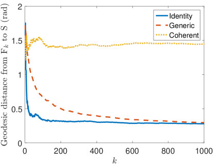
Figure 1: The numerical example described in Remark 5.

III Proof of Theorem 1

Let us first simplify the notation and introduce some helpful details. For $A\in\mathbb{R}^{n\times b}$, set

$$\mathcal{P}_{p}(A):=\sum_{i=1}^{n}\sum_{j=1}^{b}\epsilon_{i,j}A[i,j]\cdot E_{i,j},$$ (9)

where $\{\epsilon_{i,j}\}_{i,j}$ is a sequence of independent Bernoulli random variables, taking one with probability $p$ and zero otherwise. Also, $E_{i,j}\in\mathbb{R}^{n\times b}$ is the $[i,j]$-th canonical matrix in $\mathbb{R}^{n\times b}$, i.e., $E_{i,j}[i,j]=1$ is the only nonzero entry of $E_{i,j}$. Let $\Omega\subset[1:n]\times[1:b]$ be the random index set corresponding to the support of $\mathcal{P}_{p}(A)$. We set $Y=\mathcal{P}_{p}(SQ)$ and let $Y_{r}\in\mathbb{R}^{n\times b}$ be a rank-$r$ truncation of $Y$, obtained via singular value decomposition (SVD). We also let $\operatorname{Y}=\mbox{span}(Y_{r})$. Note that $\operatorname{Y}$ is a random subspace on the Grassmannian $\mathbb{G}(n,r)$.

We wish to calculate how far the true subspace S is from Fréchet expectation(s) of $\operatorname{Y}$, defined as solution(s) of the program

$$\min_{\operatorname{S}^{\prime}\in\mathbb{G}(n,r)}f\left(\operatorname{S}^{\prime}\right),\qquad f\left(\operatorname{S}^{\prime}\right):=\mathbb{E}\Big{[}d_{\mathbb{G}}\left(\operatorname{S}^{\prime},\operatorname{Y}\right)^{2}\Big{]},$$ (10)

where the expectation is with respect to the coefficient matrix $Q$ and the support $\Omega$. Let $\{\theta_{i}(\operatorname{S}^{\prime},\operatorname{Y})\}_{i=1}^{r}$ denote the principal angles between the two subspaces $\operatorname{S}^{\prime},\operatorname{Y}\in\mathbb{G}(n,r)$. It is well-known that $\{\sin(\theta_{i}(\operatorname{S}^{\prime},\operatorname{Y}))\}_{i=1}^{r}$ are in fact the singular values of $P_{\operatorname{S}^{\prime\perp}}P_{\operatorname{Y}}$, where $P_{\operatorname{A}}$ denotes the orthogonal projection matrix onto a subspace $\operatorname{A}$. Moreover,

$$d_{\mathbb{G}}\left(\operatorname{S}^{\prime},\operatorname{Y}\right)^{2}=\frac{1}{r}\sum_{i=1}^{r}\theta_{i}\left(\operatorname{S}^{\prime},\operatorname{Y}\right)^{2}=\frac{1}{r}\left\|\mbox{arcsin}\left(P_{\operatorname{S}^{\prime\perp}}P_{\operatorname{Y}}\right)\right\|_{F}^{2},$$ (11)

where $\mbox{arcsin}(\cdot)$, applied to a matrix, acts only on the singular values, leaving the singular vectors intact [23]. The geodesic distance $d_{\mathbb{G}}(\operatorname{S}^{\prime},\operatorname{Y})$ is tightly controlled as follows:

$$d_{\mathbb{G}}\left(\operatorname{S}^{\prime},\operatorname{Y}\right)^{2} =\frac{1}{r}\left\|\mbox{arcsin}\left(P_{\operatorname{S}^{\prime\perp}}P_{\operatorname{Y}}\right)\right\|_{F}^{2}\qquad\mbox{(see \eqref{eq:exp for dGR})}$$

$$\lesssim\frac{1}{r}\left\|P_{\operatorname{S}^{\prime\perp}}P_{\operatorname{Y}}\right\|_{F}^{2}\qquad\left(|\arcsin a|\leq{\pi}|a|/2\right)$$

$$\leq\left\|P_{\operatorname{S}^{\prime\perp}}P_{\operatorname{Y}}\right\|^{2},\quad\left(\mbox{rank}\left(P_{\operatorname{S}^{\prime\perp}}P_{\operatorname{Y}}\right)\leq r\right)$$ (12)

$$d_{\mathbb{G}}\left(\operatorname{S}^{\prime},\operatorname{Y}\right)^{2} =\frac{1}{r}\sum_{i=1}^{r}\theta_{i}\left(\operatorname{S}^{\prime},\operatorname{Y}\right)^{2}\qquad\mbox{(see \eqref{eq:exp for dGR})}$$

$$\geq\frac{1}{r}\sum_{i=1}^{r}\sin^{2}\left(\theta_{i}\left(\operatorname{S}^{\prime},\operatorname{Y}\right)\right)\qquad\left(|a|\geq|\sin a|\right)$$

$$=\frac{1}{r}\left\|P_{\operatorname{S}^{\prime\perp}}P_{\operatorname{Y}}\right\|_{F}^{2}.$$ (13)

In turn, (12) and (13) allow us to tightly control $f(\operatorname{S}^{\prime})$ for arbitrary $\operatorname{S}^{\prime}\in\mathbb{G}(n,r)$:

$$f\left(\operatorname{S}^{\prime}\right) =\frac{1}{r}\mathbb{E}\left[d_{\mathbb{G}}\left(\operatorname{S}^{\prime},Y\right)^{2}\right]\qquad\mbox{(see \eqref{eq:re def Fr\'{e}chet})}$$

$$\lesssim\mathbb{E}\left[\left\|P_{\operatorname{S}^{\prime\perp}}P_{\operatorname{Y}}\right\|^{2}\right],\qquad\mbox{(see \eqref{eq:bnd on d})}$$ (14)

$$f\left(\operatorname{S}^{\prime}\right) \geq\frac{1}{r}\mathbb{E}\left[\left\|P_{\operatorname{S}^{\prime\perp}}P_{\operatorname{Y}}\right\|_{F}^{2}\right].\qquad\mbox{(see \eqref{eq:lwr bnd on d})}$$ (15)

Of particular interest to us is evaluating $f(\operatorname{S})$ which, as (14) and (15) suggest, requires an estimate of the principal angle $\sin(\theta_{1}(\operatorname{S},\operatorname{Y}))=\|P_{\operatorname{S}^{\perp}}P_{\operatorname{Y}}\|$. The following result is proved in Section IV with the aid of a sharp perturbation bound, as well as basic large deviation results.

Lemma 1.

Fix $Q\in\mathbb{R}^{r\times b}$ with rank $r$ and let $\kappa(Q)$ be its condition number. Also set $\operatorname{Q}=\mbox{span}(Q^{*})$. For $\alpha\geq 1$ and except with a probability of at most $e^{-\alpha}$, it holds that

$$\left\|P_{\operatorname{S}^{\perp}}P_{\operatorname{Y}}\right\|$$

$$\lesssim\alpha\cdot\kappa(Q)\left(1\vee\sqrt{\frac{n}{b}}\right)\sqrt{\frac{r\left(\nu(\operatorname{S})\vee\mu(\operatorname{Q})\right)\log\left(n\vee b\right)}{pn}},$$

provided that

$$p\gtrsim\alpha^{2}\kappa(Q)^{2}\left(1\vee\frac{n}{b}\right){\frac{r\left(\mu\left(\operatorname{S}\right)\vee\mu(\operatorname{Q})\right)\log(n\vee b)}{n}}.$$

Lemma 1 readily translates into a bound on $f(\operatorname{S})$: For $\alpha,\widetilde{\kappa},\widetilde{\mu}_{\operatorname{Q}}\geq 1$, suppose that

$$p\gtrsim\alpha^{2}\widetilde{\kappa}^{2}\left(1\vee\frac{n}{b}\right){\frac{r\left(\mu\left(\operatorname{S}\right)\vee\widetilde{\mu}_{\operatorname{Q}}\right)\log(n\vee b)}{n}},$$ (16)

and conveniently let $\mathcal{E}$ denote the event where both $\kappa(Q)\leq\widetilde{\kappa}_{\operatorname{Q}}$ and $\mu(Q)\leq\widetilde{\mu}_{\operatorname{Q}}$ hold. Also set

$$\Delta:=\alpha\cdot\kappa(Q)\left(1\vee\sqrt{\frac{n}{b}}\right)\sqrt{\frac{r\left(\nu\left(\operatorname{S}\right)\vee\mu\left(\operatorname{Q}\right)\right)\log\left(n\vee b\right)}{pn}}.$$

and let $\mathcal{E}^{\prime}$ be the event where $\left\|P_{\operatorname{S}}^{\perp}P_{\operatorname{Y}}\right\|^{2}\leq\Delta^{2}$. Then, note that

$$f\left(\operatorname{S}\right) \lesssim\mathbb{E}\left[\left\|P_{\operatorname{S}^{\perp}}P_{\operatorname{Y}}\right\|^{2}\right]\qquad\mbox{(see \eqref{eq:upp bnd on f})}$$

$$=\mathbb{E}\left[\left\|P_{\operatorname{S}^{\perp}}P_{\operatorname{Y}}\right\|^{2}|\mathcal{E}\right]\cdot\Pr\left[\mathcal{E}\right]$$

$$\qquad+\mathbb{E}\left[\left\|P_{\operatorname{S}^{\perp}}P_{\operatorname{Y}}\right\|^{2}|\mathcal{E}^{C}\right]\cdot\Pr\left[\mathcal{E}^{C}\right]$$

$$\leq\mathbb{E}\left[\left\|P_{\operatorname{S}^{\perp}}P_{\operatorname{Y}}\right\|^{2}|\mathcal{E}\right]+\Pr\left[\mathcal{E}^{C}\right],$$ (17)

where $\mathcal{E}^{C}$ is the complement of the event $\mathcal{E}$. To bound the expectation in the last line above, let $\mathcal{E}^{\prime}$ be the event where $\left\|P_{\operatorname{S}}^{\perp}P_{\operatorname{Y}}\right\|^{2}\leq\Delta^{2}$ and note that

$$\mathbb{E}\left[\left\|P_{\operatorname{S}^{\perp}}P_{\operatorname{Y}}\right\|^{2}|\mathcal{E}\right]$$

$$=\mathbb{E}_{Q}\left[\mathbb{E}_{\Omega}\left[\left\|P_{\operatorname{S}^{\perp}}P_{\operatorname{Y}}\right\|^{2}\right]|\mathcal{E}\right]$$

$$=\mathbb{E}_{Q}\left[\mathbb{E}_{\Omega}\left[\left\|P_{\operatorname{S}}^{\perp}P_{\operatorname{Y}}\right\|^{2}|\mathcal{E}^{\prime}\right]\Pr\left[\mathcal{E}^{\prime}\right]\right.$$

$$\qquad\left.+\mathbb{E}_{\Omega}\left[\left\|P_{\operatorname{S}}^{\perp}P_{\operatorname{Y}}\right\|^{2}|\mathcal{E}^{\prime C}\right]\Pr\left[\mathcal{E}^{\prime C}\right]|\mathcal{E}\right]$$

$$\leq\mathbb{E}_{Q}\left[\Delta^{2}+e^{-\alpha}|\mathcal{E}\right]\qquad\mbox{(see Lemma \ref{lem:angle S n R})}$$

$$\leq\Delta^{2}+e^{-\alpha}$$ (18)

Substituting the bound above back into (17), we find that

$$f(\operatorname{S})$$

$$\leq\mathbb{E}\left[\left\|P_{\operatorname{S}^{\perp}}P_{\operatorname{Y}}\right\|^{2}|\mathcal{E}\right]+\Pr\left[\mathcal{E}^{C}\right]\qquad\mbox{(see \eqref{eq:added recently})}$$

$$\lesssim\Delta^{2}+e^{-\alpha}+\Pr\left[\mathcal{E}^{C}\right].\qquad\mbox{(see \eqref{eq:added recently 2})}$$ (19)

In words, when $p$ is sufficiently large, $f(\operatorname{S})$ is small. Let us next find a lower bound on $f(\cdot)$ far from $\operatorname{S}$: For an arbitrary subspace $\mbox{S}^{\prime}\in\mathbb{G}(n,r)$, we note that

$$f\left(\mbox{S}^{\prime}\right)$$

$$\geq\frac{1}{r}\mathbb{E}\left[\left\|P_{\operatorname{S}^{\prime\perp}}P_{\operatorname{Y}}\right\|_{F}^{2}\right]\qquad\mbox{(see \eqref{eq:lwr bnd on f})}$$

$$\geq\frac{1}{r}\left\|P_{\operatorname{S}^{\prime\perp}}\cdot\mathbb{E}\left[P_{\operatorname{Y}}\right]\right\|_{F}^{2}\qquad\mbox{(Jensen's ineq.)}$$

$$\geq\frac{1}{r}\left(\left\|P_{\operatorname{S}^{\prime\perp}}P_{\operatorname{S}}\right\|_{F}-\left\|P_{\operatorname{S}^{\prime\perp}}\left(P_{\operatorname{S}}-\mathbb{E}\left[P_{\operatorname{Y}}\right]\right)\right\|_{F}\right)^{2}\,\mbox{(triangle ineq.)}$$

$$\geq\frac{1}{2r}\left\|P_{\operatorname{S}^{\prime\perp}}P_{\operatorname{S}}\right\|_{F}^{2}-\frac{1}{r}\left\|P_{\operatorname{S}^{\prime\perp}}\left(P_{\operatorname{S}}-\mathbb{E}\left[P_{\operatorname{Y}}\right]\right)\right\|_{F}^{2}$$

$$\geq\frac{1}{2r}\left\|P_{\operatorname{S}^{\prime\perp}}P_{\operatorname{S}}\right\|_{F}^{2}-\frac{1}{r}\left\|P_{\operatorname{S}}-\mathbb{E}\left[P_{\operatorname{Y}}\right]\right\|_{F}^{2}$$

$$\geq\frac{1}{2}\left\|P_{\operatorname{S}^{\prime\perp}}P_{\operatorname{S}}\right\|_{F}^{2}-\mathbb{E}\left[\left\|P_{\operatorname{S}}-P_{\operatorname{Y}}\right\|_{F}^{2}\right]\qquad\mbox{(Jensen's ineq.)}$$

$$=\frac{1}{2r}\left\|P_{\operatorname{S}^{\prime\perp}}P_{\operatorname{S}}\right\|_{F}^{2}-\frac{2}{r}\mathbb{E}\left[\left\|P_{\operatorname{S}^{\perp}}P_{\operatorname{Y}}\right\|_{F}^{2}\right]$$

$$\geq\frac{1}{2r}\left\|P_{\operatorname{S}^{\prime\perp}}P_{\operatorname{S}}\right\|_{F}^{2}-2\mathbb{E}\left\|P_{\operatorname{S}^{\perp}}P_{\operatorname{Y}}\right\|^{2}\qquad\left(\mbox{rank}\left(P_{\operatorname{S}}^{\perp}P_{\operatorname{Y}}\right)\leq r\right)$$

for an absolute constant $\Cr{global}>0$. Above, we used the inequality $\left(a-b\right)^{2}\geq\frac{a^{2}}{2}-b^{2}$ for scalars $a,b$ and the fact that $\left\|P_{\operatorname{S}}-P_{\operatorname{Y}}\right\|_{F}^{2}=2\left\|P_{\operatorname{S}^{\perp}}P_{\operatorname{Y}}\right\|_{F}^{2}$. To summarize in words, $f(\operatorname{S})$ is small for large $p$ because of (19). Moreover, thanks to (LABEL:eq:lowr_bnd_on_f), we know that $f(\mbox{S}^{\prime})$ is large for any subspace $\operatorname{S}^{\prime}$ far from $\operatorname{S}$. Therefore, any minimizer of $f(\cdot)$ in (10) (namely, any Fréchet expectation $\operatorname{F}$) must be close to the true subspace S. More formally,

$$\left\|P_{\operatorname{S}^{\prime\perp}}P_{\operatorname{S}}\right\|_{F}^{2}\gtrsim\Delta^{2}+\Pr\left[\mathcal{E}^{C}\right]\Longrightarrow f\left(\operatorname{S}^{\prime}\right)>f\left(\operatorname{S}\right),$$ (20)

and, consequently,

$$\frac{1}{r}{\sum_{i=1}^{r}\sin^{2}\left(\theta_{i}\left(\operatorname{F},\operatorname{S}\right)\right)}=\frac{\left\|P_{\operatorname{F}^{\perp}}P_{\operatorname{S}}\right\|_{F}^{2}}{r}\lesssim\Delta^{2}+e^{-\alpha}+\Pr\left[\mathcal{E}^{C}\right],$$ (21)

which completes the proof of Theorem 1 after noting that $\Pr[\mathcal{E}^{C}]\leq\Pr[\kappa(Q)>\widetilde{\kappa}]+\Pr[\mu(\operatorname{Q})>\widetilde{\mu}_{\operatorname{Q}}]$, and using the fact that $|a|\leq\pi|\sin(a)|/2$ when $|a|\leq\pi/2$.

IV Proof of Lemma 1

Fix $Q\in\mathbb{R}^{r\times b}$ for now and assume $Q$ is rank-$r$. Consider the measurement matrix $Y=\mathcal{P}_{p}(SQ)\in\mathbb{R}^{n\times b}$ and let $Y_{r}\in\mathbb{R}^{n\times b}$ be a rank-$r$ truncation of $Y$, obtained via SVD, and set $\operatorname{Y}=\mbox{span}(Y_{r})$. Let also $Y_{r^{+}}:=Y-Y_{r}$ denote the residual. Note that

$$\left\|P_{\operatorname{S}^{\perp}}P_{\operatorname{Y}}\right\| =\left\|P_{\operatorname{S}^{\perp}}Y_{r}Y_{r}^{\dagger}\right\|$$

$$=\left\|P_{\operatorname{S}^{\perp}}\left(Y-Y_{r^{+}}\right)Y_{r}^{\dagger}\right\|$$

$$=\left\|P_{\operatorname{S}^{\perp}}YY_{r}^{\dagger}\right\|\qquad\left(Y_{r^{+}}Y_{r}^{*}=0\right)$$

$$\leq\left\|P_{\operatorname{S}^{\perp}}Y\right\|\cdot\left\|Y_{r}^{\dagger}\right\|$$

$$=\frac{\left\|P_{\operatorname{S}^{\perp}}Y\right\|}{\sigma_{r}\left(Y_{r}\right)}$$

$$\leq\frac{\left\|P_{\operatorname{S}^{\perp}}Y\right\|}{\sigma_{r}\left(pSQ\right)-\left\|Y_{r}-pSQ\right\|}\,\,\,\,\,\,\,\,\mbox{(Weyl's inequality)}$$

$$=\frac{\left\|P_{\operatorname{S}^{\perp}}Y\right\|}{p\cdot\sigma_{r}\left(Q\right)-\left\|Y_{r}-pSQ\right\|},\qquad\left(S^{*}S=I_{r}\right)$$ (22)

which is slightly sharper than the standard perturbation bound [29, Theorem 3], and the difference is consequential in our problem. We next control both norms in the last line above. Beginning with the numerator, we write that

$$P_{\operatorname{S}^{\perp}}Y =P_{\operatorname{S}^{\perp}}\mathcal{P}_{p}\left(SQ\right)$$

$$=P_{\operatorname{S}^{\perp}}\sum_{i,j}\epsilon_{i,j}\cdot(SQ)[i,j]\cdot E_{i,j}\qquad\mbox{(see \eqref{eq:def of R})}$$

$$=:\sum_{i,j}Z_{i,j},$$ (23)

where $\{Z_{i,j}\}_{i,j}\subset\mathbb{R}^{n\times b}$ are independent zero-mean random matrices. In order to appeal to the matrix Bernstein inequality [30], some preparation is required:

$$\nu(\operatorname{S})$$

$$=\frac{n}{r}\left\|\left[\begin{array}[]{ccc}\left\|S[1,:]\right\|_{2}&\\ &\ddots&\\ &&\left\|S[n,:]\right\|_{2}\end{array}\right]\cdot S^{\perp}\right\|^{2}\qquad\mbox{(see \eqref{eq:def of coherence})}$$ (27)

$$=\frac{n}{r}\left\|\sum_{i=1}^{n}\left\|S[i,:]\right\|_{2}^{2}\cdot P_{\operatorname{S}^{\perp}}E_{i,i}P_{\operatorname{S}^{\perp}}\right\|$$

$$\leq e\frac{n}{r}\max_{i}\left\|\left\|S[i,:]\right\|_{2}^{2}\cdot P_{\operatorname{S}^{\perp}}E_{i,i}P_{\operatorname{S}^{\perp}}\right\|$$

$$=\frac{n}{r}\max_{i}\left(\left\|S[i,:]\right\|_{2}^{2}\cdot\left\|S^{\perp}[i,:]\right\|_{2}^{2}\right),$$ (28)

$$\max_{i,j}\left\|Z_{i,j}\right\|$$

$$=\max_{i,j}\left\|\epsilon_{i,j}\cdot(SQ)[i,j]\cdot P_{\operatorname{S}^{\perp}}E_{i,j}\right\|\qquad\mbox{(see \eqref{eq:def Zs})}$$

$$\leq\max_{i,j}\left\|(SQ)[i,j]\cdot P_{\operatorname{S}^{\perp}}E_{i,j}\right\|\qquad\left(\epsilon_{i,j}\in\{0,1\}\right)$$

$$\leq\max_{i,j}\left\|S[i,:]\right\|_{2}\cdot\left\|Q[:,j]\right\|_{2}\cdot\left\|P_{\operatorname{S}^{\perp}}E_{i,j}\right\|$$

$$\leq\|Q\|\sqrt{\frac{r\mu(\operatorname{Q})}{b}}\max_{i,j}\left\|S[i,:]\right\|_{2}\cdot\left\|P_{\operatorname{S}^{\perp}}E_{i,j}\right\|\qquad\mbox{(see \eqref{eq:old coh})}$$

$$=\|Q\|\sqrt{\frac{r\mu(\operatorname{Q})}{b}}\max_{i}\left\|S[i,:]\right\|_{2}\cdot\left\|S^{\perp}[i,:]\right\|_{2}$$

$$\leq\|Q\|\sqrt{\frac{r\mu(\operatorname{Q})}{b}}\sqrt{\frac{r\nu(\operatorname{S})}{n}}=:\beta,\qquad\mbox{(see \eqref{eq:new coh simplified})}$$ (29)

$$\left\|\mathbb{E}_{\Omega}\left[\sum_{i,j}Z_{i,j}Z_{i,j}^{*}\right]\right\|$$

$$=\left\|\sum_{i,j}\mathbb{E}_{\Omega}\left[\epsilon_{i,j}^{2}\right]\cdot\left|(SQ)[i,j]\right|^{2}\cdot P_{\operatorname{S}^{\perp}}E_{i,i}P_{\operatorname{S}^{\perp}}\right\|$$

$$=\left\|\sum_{i,j}\mathbb{E}_{\Omega}\left[\epsilon_{i,j}\right]\cdot\left|(SQ)[i,j]\right|^{2}\cdot P_{\operatorname{S}^{\perp}}E_{i,i}P_{\operatorname{S}^{\perp}}\right\|\,\,\left(\epsilon_{i,j}\in\{0,1\}\right)$$

$$=p\left\|\sum_{i,j}\left|(SQ)[i,j]\right|^{2}\cdot P_{\operatorname{S}^{\perp}}E_{i,i}P_{\operatorname{S}^{\perp}}\right\|\,\,\,\left(\epsilon_{i,j}\sim\mbox{Bernoulli}(p)\right)$$

$$=p\left\|\sum_{i}\left\|S[i,:]Q\right\|_{2}^{2}\cdot P_{\operatorname{S}^{\perp}}E_{i,i}P_{\operatorname{S}^{\perp}}\right\|$$

$$\leq p\|Q\|^{2}\left\|\sum_{i}\left\|S[i,:]\right\|_{2}^{2}\cdot P_{\operatorname{S}^{\perp}}E_{i,i}P_{\operatorname{S}^{\perp}}\right\|$$

$$=p\|Q\|^{2}\frac{r\nu(\operatorname{S})}{n},\qquad\mbox{(see \eqref{eq:new coh simplified})}$$ (30)

$$\left\|\mathbb{E}_{\Omega}\left[\sum_{i,j}Z_{i,j}^{*}Z_{i,j}\right]\right\|$$

$$=\left\|\sum_{i,j}\mathbb{E}_{\Omega}\left[\epsilon_{i,j}\right]\cdot\left|(SQ)[i,j]\right|^{2}\cdot E_{j,i}P_{\operatorname{S}^{\perp}}E_{i,j}\right\|$$

$$=p\left\|\sum_{i,j}\left|(SQ)[i,j]\right|^{2}\cdot E_{j,i}P_{\operatorname{S}^{\perp}}E_{i,j}\right\|\,\,\,\,\left(\epsilon_{i,j}\sim\mbox{Bernoulli}(p)\right)$$

$$\leq p\left\|\sum_{i,j}\left|(SQ)[i,j]\right|^{2}\cdot E_{j,i}E_{i,j}\right\|$$

$$=p\left\|\sum_{i,j}\left|(SQ)[i,j]\right|^{2}\cdot E_{j,j}\right\|$$

$$=p\left\|\sum_{j}\left\|S\cdot Q[:,j]\right\|_{2}^{2}\cdot E_{j,j}\right\|$$

$$=p\left\|\sum_{j}\left\|Q[:,j]\right\|_{2}^{2}\cdot E_{j,j}\right\|\qquad\left(S^{*}S=I_{r}\right)$$

$$=p\max_{j}\left\|Q[:,j]\right\|_{2}^{2}$$

$$\leq p\|Q\|^{2}\frac{r\mu(\operatorname{Q})}{b},\qquad\mbox{(see \eqref{eq:old coh})}$$ (31)

$$\sigma^{2}$$

$$:=\left\|\mathbb{E}_{\Omega}\left[\sum_{i,j}Z_{i,j}Z_{i,j}^{*}\right]\right\|\vee\left\|\mathbb{E}_{\Omega}\left[\sum_{i,j}Z_{i,j}^{*}Z_{i,j}\right]\right\|$$

$$\leq p\|Q\|^{2}\left(1\vee\frac{n}{b}\right)\cdot\frac{r\left(\nu(\operatorname{S})\vee\mu(\operatorname{Q})\right)}{n}.\quad\,\,\,\,\mbox{(see \eqref{eq:sigma leg 1} and \eqref{eq:sigma leg 2})}$$ (32)

(In fact, using a slightly different argument, $p$ in (32) can be replaced with $p(1-p)$. However, since $p$ is typically small, this does not lead to a substantial improvement in final results and is therefore ignored here.) We are now in position to apply the matrix Bernstein inequality [30]: For $\alpha\geq 1$ and except with a probability of at most $e^{-\alpha}$, it holds that

$$\left\|P_{\operatorname{S}^{\perp}}Y\right\|$$

$$=\left\|\sum_{i,j}Z_{i,j}\right\|\qquad\mbox{(see \eqref{eq:def Zs})}$$

$$\lesssim\alpha\cdot\max\left(\log(n\vee b)\cdot\beta,\sqrt{\log(n\vee b)}\cdot\sigma\right)$$

$$\leq\alpha\|Q\|\left(1\vee\sqrt{\frac{n}{b}}\right)\cdot\max\left(\log(n\vee b)\cdot\frac{r\left(\nu(\operatorname{S})\vee\mu(\operatorname{Q})\right)}{n}\right.$$

$$\qquad\qquad\left.,\sqrt{\log(n\vee b)}\cdot\sqrt{p}\cdot\sqrt{\frac{r\left(\nu(\operatorname{S})\vee\mu(\operatorname{Q})\right)}{n}}\right)$$

$$=\alpha\|Q\|\left(1\vee\sqrt{\frac{n}{b}}\right)\cdot\sqrt{\log(n\vee b)}\cdot\sqrt{p}\cdot\sqrt{\frac{r\left(\nu(\operatorname{S})\vee\mu(\operatorname{Q})\right)}{n}},$$ (33)

when $p$ is sufficiently large. On the other hand, note that $\mathbb{E}_{\Omega}[\mathcal{P}_{p}(SQ)]=pSQ$. In fact, another application of the matrix Bernstein’s inequality proves that

$$\left\|\mathcal{P}_{p}(SQ)-pSQ\right\|$$

$$\leq C\alpha\|Q\|\left(1\vee\sqrt{\frac{n}{b}}\right)\cdot\sqrt{\log(n\vee b)}\cdot\sqrt{\frac{pr\left(\mu\left(\operatorname{S}\right)\vee\mu(\operatorname{Q})\right)}{n}},$$ (34)

for some constant $C$.

In particular, with $\kappa(Q)=\|Q\|/\sigma_{r}(Q)$ denoting the condition number of $Q$ and after taking

$$p\geq C^{2}\alpha^{2}\kappa(Q)^{2}\left(1\vee\frac{n}{b}\right){\frac{r\left(\mu\left(\operatorname{S}\right)\vee\nu(\operatorname{Q})\right)\log(n\vee b)}{n}},$$ (35)

we find that

$$\left\|\mathcal{P}_{p}(SQ)-pSQ\right\|\leq\frac{p\cdot\sigma_{r}(Q)}{2}.$$ (36)

Plugging (33) and (36) back into (22) yields that

$$\left\|P_{\operatorname{S}^{\perp}}P_{\operatorname{Y}}\right\|$$

$$\leq\frac{\left\|P_{\operatorname{S}^{\perp}}Y\right\|}{p\cdot\sigma_{r}\left(Q\right)-\left\|Y_{r}-pSQ\right\|}\qquad\mbox{(see \eqref{eq:tail bound pert})}$$

$$\leq\frac{\left\|P_{\operatorname{S}^{\perp}}Y\right\|}{p\cdot\sigma_{r}(Q)/2}\qquad\mbox{(see \ref{eq:small enough})}$$

$$\lesssim\alpha\cdot\kappa(Q)\left(1\vee\sqrt{\frac{n}{b}}\right)\cdot\sqrt{\frac{r\left(\nu(\operatorname{S})\vee\mu(\operatorname{Q})\right)\log\left(n\vee b\right)}{pn}},$$

provided that $p$ satisfies (35). The last line above uses (33). This completes the proof of Lemma 1.

References

[1]
M.K. Warmuth and D. Kuzmin.
Randomized online pca algorithms with regret bounds that are
logarithmic in the dimension.
Journal of Machine Learning Research, 9(Oct):2287–2320, 2008.
[2]
R. Arora, A. Cotter, K. Livescu, and N. Srebro.
Stochastic optimization for PCA and PLS.
In Allerton Conference on on Communication, Control, and
Computing, pages 861–868, 2012.
[3]
W. Yang and H. Xu.
Streaming sparse principal component analysis.
In Proceedings of the 32nd International Conference on Machine
Learning (ICML-15), pages 494–503, 2015.
[4]
P. van Overschee and B.L. de Moor.
Subspace identification for linear systems: Theory,
implementation, applications.
Springer US, 2012.
[5]
Z. Liu and L. Vandenberghe.
Interior-point method for nuclear norm approximation with application
to system identification.
SIAM Journal on Matrix Analysis and Applications,
31(3):1235–1256, 2009.
[6]
A. Lakhina, M. Crovella, and C. Diot.
Diagnosing network-wide traffic anomalies.
In ACM SIGCOMM Computer Communication Review, volume 34, pages
219–230. ACM, 2004.
[7]
B.A. Ardekani, J. Kershaw, K. Kashikura, and I. Kanno.
Activation detection in functional MRI using subspace modeling and
maximum likelihood estimation.
IEEE Transactions on Medical Imaging, 18(2):101–114, 1999.
[8]
D. Manolakis and G. Shaw.
Detection algorithms for hyperspectral imaging applications.
IEEE Signal Processing Magazine, 19(1):29–43, 2002.
[9]
J.P. Costeira and T. Kanade.
A multibody factorization method for independently moving objects.
International Journal of Computer Vision, 29(3):159–179, 1998.
[10]
H. Krim and M. Viberg.
Two decades of array signal processing research: the parametric
approach.
IEEE Signal processing magazine, 13(4):67–94, 1996.
[11]
L. Tong and S. Perreau.
Multichannel blind identification: From subspace to maximum
likelihood methods.
PROCEEDINGS-IEEE, 86:1951–1968, 1998.
[12]
A. Eftekhari, L. Balzano, D. Yang, and M. B. Wakin.
SNIPE for memory-limited PCA from incomplete data.
arXiv preprint arXiv:1612.00904, 2016.
[13]
L. Balzano and S.J. Wright.
Local convergence of an algorithm for subspace identification from
partial data.
Foundations of Computational Mathematics, 15(5):1279–1314,
2015.
[14]
I. Mitliagkas, C. Caramanis, and P. Jain.
Streaming PCA with many missing entries.
Preprint, 2014.
[15]
Y. Hong, X. Yang, R. Kwitt, M. Styner, and M. Niethammer.
Regression uncertainty on the Grassmannian.
In Proceedings of the AISTATS Conference, 2017.
[16]
S. Chatterjee.
Matrix estimation by universal singular value thresholding.
The Annals of Statistics, 43(1):177–214, 2015.
[17]
R. H. Keshavan, A. Montanari, and S. Oh.
Matrix completion from a few entries.
IEEE Transactions on Information Theory, 56(6):2980–2998,
2010.
[18]
R.S. Ganti, L. Balzano, and R. Willett.
Matrix completion under monotonic single index models.
In Advances in Neural Information Processing Systems, pages
1873–1881, 2015.
[19]
R. Chakraborty and B.C. Vemuri.
Recursive Fréchet mean computation on the Grassmannian and
its applications to computer vision.
In Proceedings of the IEEE International Conference on Computer
Vision, pages 4229–4237, 2015.
[20]
H. Salehian, R. Chakraborty, E. Ofori, D. Vaillancourt, and B.C. Vemuri.
An efficient recursive estimator of the Fréchet mean on a
hypersphere with applications to medical image analysis.
Mathematical Foundations of Computational Anatomy, 2015.
[21]
R. Chakraborty, S. Hauberg, and B. C. Vemuri.
Intrinsic Grassmann averages for online linear and robust subspace
learning.
arXiv preprint arXiv:1702.01005, 2017.
[22]
P-A Absil, Robert Mahony, and Rodolphe Sepulchre.
Riemannian geometry of grassmann manifolds with a view on algorithmic
computation.
Acta Applicandae Mathematica, 80(2):199–220, 2004.
[23]
G.H. Golub and C.F. Van Loan.
Matrix computations.
Johns Hopkins Studies in the Mathematical Sciences. Johns Hopkins
University Press, 2013.
[24]
M. Frechét.
Les élménts aléleatoires de nature quelconque dans un
espace distancié.
Annales de l’institut Henri Poincaré,
10:215 310, 1948.
[25]
H. Karcher.
Riemannian center of mass and mollifier smoothing.
Communications on Pure and Applied Mathematics, 30(5):509–541,
1977.
[26]
Y. Chen.
Incoherence-optimal matrix completion.
IEEE Transactions on Information Theory, 61(5):2909–2923,
2015.
[27]
R. Vershynin.
Introduction to the non-asymptotic analysis of random matrices.
arXiv preprint arXiv:1011.3027, 2010.
[28]
I.M. Johnstone and A.Y. Lu.
On consistency and sparsity for principal components analysis in high
dimensions.
Journal of the American Statistical Association, 2012.
[29]
P. Wedin.
Perturbation bounds in connection with singular value decomposition.
BIT Numerical Mathematics, 12(1):99–111, 1972.
[30]
J.A. Tropp.
User-friendly tail bounds for sums of random matrices.
Foundations of computational mathematics, 12(4):389–434, 2012.