Post-Newtonian dynamical modeling of supermassive black holes in galactic-scale simulations

Abstract

We present KETJU, a new extension of the widely-used smoothed particle hydrodynamics simulation code GADGET-3. The key feature of the code is the inclusion of algorithmically regularized regions around every supermassive black hole (SMBH). This allows for simultaneously following global galactic-scale dynamical and astrophysical processes, while solving the dynamics of SMBHs, SMBH binaries and surrounding stellar systems at sub-parsec scales. The KETJU code includes Post-Newtonian terms in the equations of motions of the SMBHs which enables a new SMBH merger criterion based on the gravitational wave coalescence timescale pushing the merger separation of SMBHs down to $\sim 0.005\ \rm pc$. We test the performance of our code by comparison to NBODY7 and rVINE. We set up dynamically stable multi-component merger progenitor galaxies to study the SMBH binary evolution during galaxy mergers. In our simulation sample the SMBH binaries do not suffer from the final-parsec problem, which we attribute to the non-spherical shape of the merger remnants. For bulge-only models, the hardening rate decreases with increasing resolution, whereas for models which in addition include massive dark matter halos the SMBH binary hardening rate becomes practically independent of the mass resolution of the stellar bulge. The SMBHs coalesce on average 200 Myr after the formation of the SMBH binary. However, small differences in the initial SMBH binary eccentricities can result in large differences in the SMBH coalescence times. Finally, we discuss the future prospects of KETJU, which allows for a straightforward inclusion of gas physics in the simulations.

1. Introduction

There is ubiquitous evidence for the presence of supermassive black holes (SMBHs) with masses in the range of $M=10^{6}-10^{10}M_{\odot}$ in the centers of all massive galaxies in the local Universe (e.g. Kormendy & Richstone 1995; Ferrarese & Ford 2005; Kormendy & Ho 2013). In addition, there is a strong suggestion of a co-evolution of SMBHs and their host galaxies as manifested in the surprisingly tight relations between the SMBH masses and the fundamental properties of the galactic bulges that host them, e.g. the bulge mass (Magorrian & et al., 1998; Häring & Rix, 2004) and the bulge stellar velocity dispersion (Gebhardt et al., 2000; Ferrarese & Merritt, 2000; Tremaine et al., 2002).

In the hierarchical picture of structure formation, galaxies grow bottom-up through mergers and gas accretion (White & Rees, 1978). Massive, slowly-rotating early-type galaxies, that are expected to host the largest SMBHs in the Universe, are believed to have assembled through a two-stage process. The early assembly is dominated by rapid in situ star formation fueled by cold gas flows and hierarchical merging of multiple star-bursting progenitors, whereas the later growth below redshifts of $z\lesssim 2-3$ is dominated by a more quiescent phase of accretion of stars formed mainly in progenitors outside the main galaxy (e.g. Naab et al. 2009; Oser et al. 2010; Feldmann et al. 2011; Johansson et al. 2012; Wellons et al. 2015; Rodriguez-Gomez et al. 2016; Qu et al. 2016). See also Naab & Ostriker (2016) for a review.

This hierarchical formation process will result in situations with multiple SMBHs in the same stellar system (e.g. Begelman et al. 1980; Volonteri et al. 2003). These SMBHs will subsequently sink to the center of the galaxy due to dynamical friction from stars and gas and form a wide gravitationally bound binary with a semi-major axis of $a\sim 10$ pc. Next, the semi-major-axis of the binary will shrink (’harden’) due to the interaction of the binary with the stellar background. A star crossing at a distance of the order of the semi-major axis of the binary will experience a complex three-body interaction with the binary and carry away energy and angular momentum from the SMBH binary system (eg. Hills & Fullerton 1980). If the population of stars with centrophilic orbits is not depleted, the binary will harden at an approximately constant rate:

$$\frac{\mathrm{d}}{\mathrm{d}t}\left(\frac{1}{a}\right)\propto\frac{G\rho_{\star}}{\sigma_{\star}},$$ (1)

assuming a constant stellar density $(\rho_{\star})$ and velocity dispersion $(\sigma_{\star})$ at the center of the galaxy (Quinlan, 1996). If the center-crossing (or ’SMBH loss cone’) orbital population is depleted, the binary hardening is halted. This so-called final-parsec problem is persistently present in simulations of isolated collisionless spherically symmetric stellar systems (Milosavljević & Merritt, 2001, 2003).

Recent numerical work suggests that the problem is less severe or might even be nonexistent in simulations of triaxial (Berczik et al., 2006) and axisymmetric galaxies (Khan et al., 2013), for which the added asymmetric perturbations in the gravitational potential are able to refill the loss cone by repopulating centrophilic stellar orbits. Similarly, the merger of two galaxies will break the symmetry of the galactic potentials resulting in a more efficient refilling of the loss cone and thus potentially avoiding the final-parsec problem (Preto et al., 2011; Khan et al., 2011, 2012). However, even in simulations that avoid the final-parsec problem the loss-cone filling rate is affected by the enhanced two-body relaxation timescale, especially in simulations with $N\lesssim 10^{6}$ particles (Vasiliev et al., 2015). Recently, Gualandris et al. (2016) also studied the collisionless loss-cone repopulation in triaxial galaxies without SMBHs using an accurate fast multipole method and found that for particle numbers $N<10^{7}$, the loss-cone filling rate is mildly $N$-dependent, whereas the rate becomes practically independent of $N$ for particle numbers above $N\sim 10^{7}$.

Recent observations show that even early-type galaxies have non-negligible gas reservoirs of cold gas in their central regions (Young et al., 2011; Davis et al., 2013). The inclusion of gas in the simulations tends to result in non-axisymmetric gas torques and a remnant that is denser in the central regions due to the dissipative nature of the gaseous component. Both of these effects facilitate rapid hardening of a SMBH binary and might help in solving the final-parsec problem (Armitage & Natarajan, 2005; Mayer et al., 2007). This is especially true at high redshifts where very gas-rich mergers are expected to occur frequently (Khan et al., 2016). Indeed, there is observational evidence for the presence of massive black holes from strong nuclear outflows at $z\sim 1-2$ (Genzel et al., 2014). However, the results from hydrodynamical simulations depend sensitively on the adopted feedback and star formation model, and thus we caution that it is not yet clear, whether the inclusion of gaseous component on its own is sufficient for solving the final-parsec problem (see e.g. Chapon et al. 2013).

If the final-parsec problem is avoided, the loss of orbital energy eventually becomes dominated by the emission of gravitational waves at very small centiparsec binary separations with a strong dependence on the binary eccentricity. Recently, this process was spectacularly confirmed by the direct detection of gravitational waves from a stellar mass BH binary system by Abbott et al. (2016). Future space-borne low-frequency laser interferometers are expected to detect a similar signal from supermassive black hole binary systems (e.g. Amaro-Seoane et al. 2012).

To model the dynamics of SMBHs in galaxy mergers, one would ideally run a simulation that simultaneously resolves the global kpc-scale dynamics of the merger and the subparsec evolution of the SMBH binary. This is a very ambitious goal and typically only one of these scales has been properly resolved and modeled in any given simulation. In the past decade there has been significant progress in simulating both galaxy mergers and the full cosmological evolution of galaxies including the effects of SMBHs initially using smoothed particle hydrodynamics (SPH) (e.g.Di Matteo et al. 2005; Springel et al. 2005; Sijacki et al. 2007; Johansson et al. 2009a, b; Booth & Schaye 2009; Choi et al. 2012) and later also using both adaptive-mesh refinement (AMR) (e.g. Kim et al. 2011; Martizzi et al. 2012; Dubois et al. 2012) and moving mesh techniques (e.g. Vogelsberger et al. 2013; Costa et al. 2014; Sijacki et al. 2015; Kelley et al. 2017a, b). These simulations allow for a large number of particles and are very successful in capturing the global structure of gas and stars in the galaxies. In addition, they are able to approximatively follow additional astrophysical processes by including sophisticated subresolution models for gas cooling, star formation, metal enrichment and the feedback from SMBHs and evolving stellar populations.

However, the fundamental limitation of this approach is that only a limited number of particles or grid cells sample the underlying smooth gravitational potential and by necessity the gravitational force must be softened to reduce the graininess of the potential. The softening length or equivalently the size of the minimum grid cell sets a natural resolution limit, below which the dynamics, such as the close two-body encounters with a massive SMBH cannot be modeled accurately. This also leads to uncertainties in dynamical friction timescales of SMBHs. A possibility that circumvents this problem is the addition of a subresolution drag force term into the equations of motion of the sinking SMBH that accounts for the unresolved encounters of the SMBH and the field stars. This method is particularly well suited for cosmological simulations, which typically have low spatial resolution (Tremmel et al., 2015).

Gravitational softening will also affect the density and velocity profiles of stars in the centers of galaxies, which strongly interact with the SMBHs. Finally the hardening and merging timescales of binary SMBHs are also plagued by large uncertainties and the common ’a priori’ assumption often taken in these models is that both the hardening and merging of SMBHs happens rapidly, with the actual implementation then proceeding through a subresolution model with limited predictive power.

An alternative approach is to calculate the gravitational force directly by summing exactly the force from every particle on every particle. This method is computationally expensive, but allows in combination with high-order integrators for a very accurate calculation of the gravitational forces. It is widely used to simulate collisional N-body systems (e.g. Aarseth 1999). This method does not require gravitational softening but the computational time scales steeply with the particle number $\mathcal{O}(N^{2})$ as opposed to tree and mesh codes, which typically scale as $\mathcal{O}(N\log N)$. In addition it is not straightforward to model the gaseous component present in galaxies in a pure N-body code and combined with the limited number of particles ($N\sim 10^{6}$, Wang et al. 2016) this limits the applicability of these codes for a self-consistent treatment of SMBH dynamics in a full galactic environment. Thus, owing to these inherent limitations current numerical simulations with N-body codes have typically only explored separate aspects of the full problem by limiting themselves to studies of SMBH binary dynamics in the centers of isolated galaxies or merger remnants, with the surrounding galaxy often represented by idealized initial conditions (e.g. Milosavljević & Merritt 2001, 2003; Berczik et al. 2006; Preto et al. 2011; Khan et al. 2011, 2013; Gualandris & Merritt 2012; Vasiliev et al. 2014; Holley-Bockelmann & Khan 2015). An important distinction to also keep in mind is the difference between the force accuracy of a simulation and the actual simulation accuracy that also depends on how accurately the orbits of the particles can be integrated. A recent paper by Dehnen (2014) demonstrated that a suitably tuned fast multipole method is capable of delivering a force accuracy comparable to that of a direct-summation code, while still retaining a very efficient $\mathcal{O}(N)$ scaling. However, for our purposes in addition to an accurate force calculation, it is also of paramount importance that we are able to accurately integrate the equations of motion without softening and to resolve arbitrarily close encounters in the vicinity of the SMBHs.

The main goal of this article is to present and test our new code that attempts to combine the best aspects of the two numerical approaches. Our code KETJU (the word for ’chain’ in Finnish) combines an algorithmic chain regularization (AR-CHAIN) method to efficiently and accurately compute the dynamics close to SMBHs with the fast and widely used tree code GADGET-3  (Springel, 2005) for the calculation of the global galactic dynamics. The performance of normal GADGET-3 can be substandard in situations that require high dynamical precision due to the insufficient precision of the tree force calculation (see e.g. Gualandris et al. 2016). Some of these problems can be mitigated by setting the internal accuracy parameters of GADGET-3 to very high values, significantly beyond their usual nominal values. In addition in our KETJU code the strongest interactions between particles will be resolved within the regularized algorithmic chain region, and not treated by standard GADGET-3. The main advantage of building KETJU on the GADGET-3 platform is that it enables the use of a rich set of astrophysical cooling and feedback models for future KETJU runs that also include a gaseous component.

A similar hybrid approach of combining a tree code with a regularization algorithm was originally implemented by Jernigan & Porter (1989) and McMillan & Aarseth (1993). Oshino et al. (2011) and Iwasawa et al. (2015) also both combined the tree algorithm with a direct summation code, however without the inclusion of regularization, whereas the BRIDGE framework developed by Fujii et al. (2007) allows for the combination of different types of N-body codes. For our purposes the most relevant precursor code is the rVINE code (Karl et al., 2015), which is very similar in spirit and functionality to our code. In rVINE an algorithmically regularized region is inserted around a single SMBH with this structure embedded in the VINE code, which is an OpenMP-parallelized tree/SPH code employing a binary tree algorithm (Wetzstein et al., 2009; Nelson et al., 2009). Although similar to rVINE, there are significant differences and improvements in the KETJU code detailed in §2 and §3. As opposed to rVINE, the KETJU code allows for multiple regularized chains with an individual chain system for each SMBH particle. In addition, the KETJU code includes Post-Newtonian (PN) correction terms up to order PN3.5, which in principle allows for accurate dynamics valid down to $\sim 10$ Schwarzschild radii.

We begin this article by covering the structure of the chain subsystems in §2 and describe how they are integrated into the GADGET-3 code. Next, we present the properties of the algorithmic chain regularization method in §3. The intricate details of the algorithms used in the code are discussed in Appendices A and B. In §4 we test and calibrate our code against rVINE and the direct summation code NBODY7. The performance and scalability of the code are discussed in §5. In §6 we use the KETJU code to study the resolution dependence of the SMBH hardening rates in merger simulations of both two- and three-component galaxy models. We discuss our results and plans for the future in §7 and finally present our conclusions in §8.

2. Regularized subsystems in Gadget-3

2.1. The chain subsystem

In the standard GADGET-3 code (Springel, 2005) the gravitational accelerations of N-body particles are computed using either a pure tree algorithm or a hybrid tree-mesh TreePM algorithm. In the TreePM method, the gravitational tree is used to compute the short-range forces while an efficient particle mesh method is used for the long-range component. Hereafter, these two force calculation procedures are referred to simply as the tree method.

GADGET-3 propagates simulation particles using a symplectic kick-drift-kick (KDK) leapfrog scheme with individual adaptive timesteps (Springel, 2005). To integrate the regularized AR-CHAIN algorithm in the GADGET-3 code, we must first select a subset of particles from the complete set of simulation particles. This regularized subset of particles is excluded from the GADGET-3 tree force calculation and the standard leapfrog propagation. These particles are instead propagated using the AR-CHAIN integrator of KETJU (hereafter, chain integration). The chain integration procedure is presented thoroughly in the next section.

We divide the simulation particles into three categories according to their type and distance to SMBH particles:

1. Chain particles: all the SMBH particles and the stellar particles which lie in the immediate vicinity of a SMBH particle. The SMBH and the surrounding stellar particles form a chain subsystem. Note that in the current implementation gas and dark matter particles cannot enter the chain subsystems.

2. Perturber particles: all the simulation particles which induce a strong tidal perturbation on a chain subsystem. These particles feel the tree force and are propagated using the GADGET-3 leapfrog, but in addition they receive a correction to their accelerations from a nearby chain subsystem.

3. Tree particles: simulation particles that are far away from any of the SMBH particles and are thus treated as ordinary GADGET-3 particles with respect to the force calculation.

We have implemented a distance-based selection criterion for chain subsystem members, in which the chain radius of a SMBH ($\bullet$) depends on the mass of the SMBH:

$$\frac{r_{\mathrm{chain}}}{1\text{ kpc}}=\lambda\times\frac{M_{\bullet}}{10^{10}M_{\odot}},$$ (2)

where $\lambda$ is a user specified dimensionless input parameter. Note that using this definition the chain radius of a SMBH remains constant in simulations with no black hole mass accretion or mergers.

After the radius of a SMBH has been set, we select the members of a chain subsystem. A stellar particle ($\star$) belongs to a chain subsystem of a SMBH if

$$\|\boldsymbol{r}_{\star}-\boldsymbol{r}_{\bullet}\|<r_{\mathrm{chain}}.$$ (3)

For a schematic illustration of a chain subsystem among tree particles, see Fig. 1.

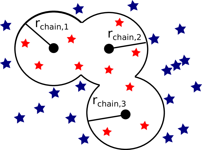
Figure 1.— An illustration of the chain subsystem with three SMBHs (black filled circles) and ten stellar chain members (red stars). The blue stars outside the SMBHs’ chain radii act as perturbing particles.

The individual chain particles are removed from the tree force calculation. However, the center-of-mass (CoM) of the chain subsystem is placed into the tree structure as a ’macro’ particle, with the combined mass of all its chain particles. This macro particle acts as an ordinary collisionless tree particle in the simulation.

The macro particle is an ordinary GADGET-3 tree particle and must have a non-zero gravitational softening length. GADGET-3 uses as a gravitational softening kernel the Monaghan-Lattanzio spline kernel (Monaghan & Lattanzio, 1985), which is exactly Newtonian outside the softening length $h_{\mathrm{ML}}$. The usually quoted Plummer-equivalent softening length $\epsilon$, which is used to set the softening lengths of simulation particles, is related to this quantity through $h_{\mathrm{ML}}=2.8\times\epsilon$ (Springel et al., 2001). Thus, we enforce the condition

$$r_{\mathrm{chain}}>2.8\times\epsilon$$ (4)

for the chain radius and the Plummer-equivalent gravitational softening length in order to ensure that the mutual gravitational interactions of stars and SMBHs are never softened in KETJU.

The chain subsystems are initialized at the beginning of the simulation, after which the status of chain particles is updated after every chain integration interval. If, at the next timestep, a chain particle has propagated outside of the chain radius of a SMBH, an escape event occurs and the chain particle is restored to the tree. If there are multiple SMBHs in a single chain, we check the escape condition for all chain particle - SMBH pairs separately. The absorption of new particles into a chain subsystem is performed similarly. An absorption event occurs if a tree particle enters the chain radius of a SMBH. The center-of-mass properties and the total mass of the macro particles are updated after both absorption and escape events. We terminate a chain subsystem if the SMBH is the only remaining chain member particle, i.e. $N_{\mathrm{c}}<2$. A new active chain subsystem is initialized if stellar particles are found inside the chain radius of a SMBH.

2.2. Tidal perturbations and force corrections

In addition to internal forces, the dynamics of the particles in a chain subsystem is affected by external gravitational forces $\boldsymbol{f}_{\mathrm{i}}$. These external forces are dominated by the closest neighboring tree particles which are not chain subsystem members. We define and select these perturber particles of a subsystem with a tidal criterion before every chain integration. A tree particle, labeled with index $j$, is selected as a perturber of a chain subsystem if the condition

$$\|\boldsymbol{r}_{j}-\boldsymbol{r}_{\bullet}\|<\gamma\times r_{\mathrm{chain}}\left(\frac{m_{\mathrm{j}}}{M_{\bullet}}\right)^{1/3}=r_{\mathrm{pert,j}}$$ (5)

is satisfied with any of the SMBHs in the particular chain subsystem. Here $\gamma$ is a user-defined tidal parameter and $r_{\mathrm{chain}}$ is the SMBH chain radius defined in Eq. (2). In the case of equal-mass perturber particles, the perturber radius is identical for all the particle species. The tidal parameter $\gamma$ is chosen as such that the perturber radius is a few times the chain radius of the SMBH. For an illustration of a perturbed subsystem see Fig. 2. In the case of unequal-mass particles, more massive particles can become perturbers even if they lie further away from the SMBH than lighter simulation particles and thus there are several perturber radii. The user-defined parameters in KETJU are listed in Table 1 with their typical values from simulations appearing in §6.

Table 1User-defined KETJU parameters with typical values in the simulations from §6.

Parameter	Description	Numerical value
$\lambda$	Sets the chain radius	1.8
$\gamma$	Sets the perturber radius	25
$\eta_{\mathrm{GBS}}$	AR-CHAIN integrator accuracy	$10^{-6}$

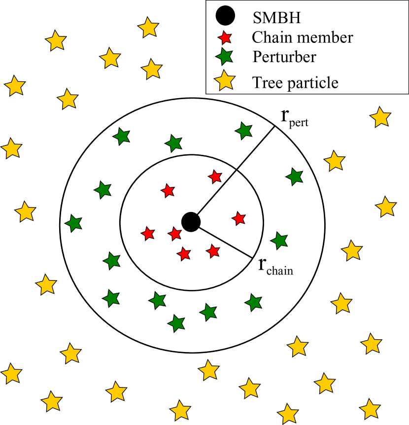
Figure 2.— An illustration of a chain subsystem with a single SMBH (the black filled circle), chain particles (red stars), perturbing tree particles (green stars) and ordinary tree particles (yellow stars). The chain radius of the SMBH is marked with $r_{\mathrm{chain}}$ and the radius containing the perturbers with $r_{\mathrm{pert}}$. Note that here we assume equal-mass tree particles so there is a single perturber radius.

During the chain integration, the external force perturbations $\boldsymbol{f}_{\mathrm{i}}$ are computed using perturber positions, as described in Algorithm 2 in Appendix B. As the AR-CHAIN integrator leapfrogs several regularized substeps during a single tree timestep and the perturber positions are obtained at the beginning of the timestep, we predict both the positions of the macroparticle and the perturber particles using a simple quadratic extrapolation. In addition, we also include the force contribution of distant tree particles as a far-field perturbation which is kept constant during the chain integration. In general, the tree force calculation does not resolve the subresolution dynamics in the chain subsystems. However, in order to satisfy Newton’s third law, perturber particles receive an extra force correction from the resolved chain after the completion of the Gadget-3 tree force calculation. The procedure is as follows. First, we subtract the contribution of the macro particle from the acceleration of the perturber particle. Then, we resolve the positions of the chain particles and compute the correction for the acceleration of the perturber using the softened direct summation method employing the Monaghan–Lattanzio cubic spline kernel (Monaghan & Lattanzio, 1985) used in standard Gadget-3. If a tree particle perturbs multiple chain subsystems, it receives a force correction from all of them. In addition, all macro particles in the tree receive a force correction due to the perturber forces on the resolved individual particles in the chain subsystem. To sum up, the internal structure of the chain subsystems in visible to the nearby perturbing tree particles. For faraway tree particles the chain subsystems appear as a single macro particles. However, this is not a problem since treating distant simulation particles using a low-order multipole expansion is in fact the essence of the tree force calculation itself (e.g. Barnes & Hut 1986). As the force correction computation scales proportionally to the number of chain particles and perturber particles, $\mathcal{O}{(N_{\mathrm{c}}\times N_{\mathrm{p}})}$, the perturber tidal parameter $\gamma$ should be selected carefully in order to optimize both code accuracy and the resulting computational cost. In this paper, we follow the general rule of thumb that

$$r_{\mathrm{pert}}\geq 2\times r_{\mathrm{chain}},$$ (6)

i.e. the perturber radius is at least twice the chain radius of the SMBH for every particle type in the simulation.

2.3. Timestepping with chain

In GADGET-3, the timestep of a collisionless particle is set to

$$\Delta t_{\mathrm{grav}}=\left(\frac{2\eta\epsilon}{|\boldsymbol{a}|}\right)^{1/2},$$ (7)

in which $\eta$ is the user-defined error tolerance parameter, $\epsilon$ is the gravitational softening length and $\boldsymbol{a}$ is the acceleration of the particle. In addition, all timesteps in GADGET-3 are discretized as power of two subdivisions of the global tree timestep (Springel, 2005).

In KETJU, the timestep criterion is modified slightly. All SMBH particles are placed on the smallest active level in the global timestep hierarchy. In addition, all the particles escaping from the chain are set to the smallest tree timestep level. The chain time integration is performed within GADGET-3’s KDK integration cycle in the following way. The subsystem/tree memberships of the simulation particles are updated at the beginning of every integration cycle. The macroparticles are propagated as ordinary tree particles while the chain subsystems are propagated after the drift operation, before updating accelerations of the active tree particles. The force corrections from the resolved macroparticles are computed after the acceleration calculation.

2.4. Multiple chain subsystems

As KETJU allows for multiple chain systems in a single simulation, it is possible for two chain subsystems to first perturb each other and then eventually merge. The tidal perturbations from one chain subsystem on another are treated in the following way. We resolve the macro particle into its constituent chain particles and treat them as described in §2.2. Finally, we merge the chain subsystems labeled $i$ and $j$ into a single subsystem if the volumes occupied by the chain systems overlap:

$$\|\boldsymbol{r}_{\mathrm{\bullet},i}-\boldsymbol{r}_{\mathrm{\bullet},j}\|<r_{\mathrm{chain},i}+r_{\mathrm{chain},j}$$ (8)

while the center-of-mass separation of the subsystems is decreasing, i.e.

$$\left(\boldsymbol{r}_{\mathrm{\bullet},i}-\boldsymbol{r}_{\mathrm{\bullet},j}\right)\cdot\left(\boldsymbol{v}_{\mathrm{\bullet},i}-\boldsymbol{v}_{\mathrm{\bullet},j}\right)<0.$$ (9)

We test for these conditions for all the chain subsystems at every GADGET-3 timestep. Likewise, we split a chain subsystem into two new subsystems if

$$\|\boldsymbol{r}_{\mathrm{\bullet},i}-\boldsymbol{r}_{\mathrm{\bullet},j}\|>r_{\mathrm{chain},i}+r_{\mathrm{chain},j}$$ (10)

and the splitting SMBH $j$ is receding from all the SMBHs in the original subsystem, i.e. the condition

$$\left(\boldsymbol{r}_{\mathrm{\bullet},i}-\boldsymbol{r}_{\mathrm{\bullet},j}\right)\cdot\left(\boldsymbol{v}_{\mathrm{\bullet},i}-\boldsymbol{v}_{\mathrm{\bullet},j}\right)>0$$ (11)

must be fulfilled for every pair of SMBHs $i\neq j$.

2.5. Particle mergers

In the standard GADGET-3 implementation (Springel et al., 2005), the SPH kernel of the code is also used to compute the gas density around the SMBHs. In addition, the size $h$ of the kernel also defines the SMBH merging criterion. Two SMBHs merge if they come within a distance of $h$ of each other and the relative speed of the SMBHs is below the local sound speed. This typically occurs at SMBH separations of the order of tens or hundreds of parsecs (e.g. Mayer et al. 2007; Johansson et al. 2009a). Because the gravitational forces in the chain subsystems are not softened, we are able to follow the orbital evolution of a SMBH binary to separations well below the gravitational softening length $\epsilon$ of the tree calculation, whereas in a softened simulation the binary would stall at the softening length. Since we can also resolve arbitrarily close encounters between two SMBHs and between SMBHs and stellar particles, a more refined criterion for mergers between SMBHs and SMBHs and stellar particles is now required.

If Post-Newtonian corrections of the order PN2.5 or higher are included, the semi-major axis of a point mass binary will shrink due to the loss of orbital energy caused by gravitational wave emission. The time evolution of the orbital semi-major axis, $a$, can be approximated by the analytical formula of Peters & Mathews (1963) valid at PN2.5:

$$\dot{a}=-\frac{64}{5}\frac{G^{3}M_{\bullet,1}M_{\bullet,2}(M_{\bullet,1}+M_{\bullet,2})}{c^{5}a^{3}}\frac{1+\frac{73}{24}e^{2}+\frac{37}{96}e^{4}}{(1-e^{2})^{7/2}},$$ (12)

where $M_{\bullet,1}$ and $M_{\bullet,2}$ are the masses of the two SMBHs and $e$ is the eccentricity of the SMBH binary. Since $\dot{a}\propto-a^{-3}$, the coalescence timescale can be approximated by

$$t_{c}\sim-\frac{a}{4\dot{a}},$$ (13)

if constant eccentricity is assumed.

For each bound SMBH binary, we compute the orbital elements and the coalescence timescale using Eq. (13) before each global GADGET-3 timestep. We compare the coalescence timescale $t_{\mathrm{c}}$ with the current tree timestep $\Delta t_{\text{tree}}$ multiplied by a temporal safety factor $s_{1}>1$. If $t_{\mathrm{c}}<s_{1}\Delta t_{\text{tree}}$, we merge the SMBHs instantly during this timestep. The same coalescence criterion is applied to the stellar particles bound to a SMBH as well. The safety factor is necessary, since Eq. (13) only gives an approximation to the coalescence timescale, and the exact dynamics might bring the particles to a collision within $\Delta t_{\text{tree}}$ even though fiducially $t_{\mathrm{c}}>\Delta t_{\text{tree}}$. We set $s_{1}=2$ in the code to ensure that this unphysical behavior does not take place. For the simulations presented in this study, the expected absolute error in the SMBH merger timescale is conservatively a few times the length of a typical timestep $\sim$ 0.001 Myr. The typical SMBH merger separation in KETJU is of the order of a few hundred AU, which is three to four orders of magnitude below the typical merger separations in GADGET-3 simulations.

We further enforce a minimum distance between two particles. For a SMBH-SMBH pair, we use a multiple of the sum of the Schwarzschild radii of the particles and set

$$r_{\text{min,S}}=6\left(\frac{2GM_{\bullet,1}}{c^{2}}+\frac{2GM_{\bullet,2}}{c^{2}}\right).$$ (14)

This criterion is based on standalone tests with the AR-CHAIN integrator, which indicate that the Post-Newtonian dynamics is still numerically well-behaved at these distances. For a pair consisting of a SMBH and a stellar particle, we use

$$r_{\text{min,T}}=\max\left\{r_{\text{min,S}},\,\,s_{2}R_{\odot}\left(\frac{M_{\bullet}}{M_{\odot}}\right)^{1/3}\right\},$$ (15)

where $s_{2}>1$ is a spatial safety factor and $M_{\odot}$ and $R_{\odot}$ are the solar mass and radius, respectively. This criterion is motivated by the usual definition for the stellar tidal disruption radius, $r_{\text{TDE}}\sim(M_{\bullet}/m_{\star})^{1/3}R_{\star}$, assuming $R_{\star}=(m_{\star}/M_{\odot})^{1/3}R_{\odot}$ for the stellar particles. For $s_{2}\sim 1$, the criterion reduces exactly to the tidal disruption distance (e.g. Kesden, 2012). To enforce larger separations well above the tidal disruption distance, we set $s_{2}=10$ in the code. This was motivated by the fact that the PN-corrections were found to be occasionally numerically unstable in the case of two-body collisions, combined with the fact that collisions are checked for before each tree timestep using a linear prediction of the particle orbits. This linear prediction gives the condition

$$2t\,\boldsymbol{r}_{12}\cdot\boldsymbol{v}_{12}+\boldsymbol{r}_{12}\cdot\boldsymbol{r}_{12}-r_{\text{min}}^{2}=0,$$ (16)

where $\boldsymbol{r}_{12}=\boldsymbol{r}_{2}-\boldsymbol{r}_{1}$ and $\boldsymbol{v}_{12}=\boldsymbol{v}_{2}-\boldsymbol{v}_{1}$ are the relative positions and velocities of the particle pair. If Eq. (16) has a solution with $t\in[0,\Delta t_{\text{tree}}]$, we merge the particles instantly.

The actual merger of the particles is performed using the equations

$$M =M_{1}+M_{2}$$ (17)

$$\boldsymbol{r} =(M_{1}\boldsymbol{r}_{1}+M_{2}\boldsymbol{r}_{2})/M$$ (18)

$$\boldsymbol{v} =(M_{1}\boldsymbol{v}_{1}+M_{2}\boldsymbol{v}_{2})/M$$ (19)

$$\boldsymbol{L} =\frac{M_{1}M_{2}}{M}\boldsymbol{r}_{12}\times\boldsymbol{v}_{12}$$ (20)

$$\boldsymbol{S} =\boldsymbol{L}+\boldsymbol{S}_{1}+\boldsymbol{S}_{2}.$$ (21)

This ensures the conservation of Newtonian linear momentum and angular momentum $|\boldsymbol{L}|$. We note here that KETJU can follow the spin $(\boldsymbol{S})$ evolution of all stellar and black hole particles. The spin state of the particles is only affected by the PN corrections, through Eq. (26), and for black holes also by the merger Eq. (21). However, in the simulations run in this study, all particle spins are initialized to zero. While the stellar spins remain zero at all times, the black hole spins also never attain a significant magnitude in the simulation.

3. The regularized integrator

3.1. Algorithmic chain regularization

The regularized dynamics in KETJU is based on a novel reimplementation of the AR-CHAIN algorithm (Mikkola & Merritt, 2008) written in the C programming language. Below we will briefly outline the algorithm. For a more involved description, see Mikkola & Aarseth (1993) and Mikkola & Merritt (2006, 2008). The algorithm has three main aspects: algorithmic regularization, the use of relative distances to reduce round-off errors, and extrapolation to obtain high numerical accuracy in orbit integrations.

Algorithmic regularization works by transforming the equations of motion into a form where integration by the common leapfrog method yields exact orbits to within numerical precision for a Newtonian two-body problem, including two-body collisions. This is achieved by introducing a new fictitious time as an independent variable in order to circumvent the collision singularity that plagues the Newtonian equations of motion. For mathematical details of the time transformation procedure, see Appendix A.

The second aspect of the regularization scheme is the use of relative positions in the numerical calculations to reduce the often significant effect of round-off error. The relative positions, or chain vectors, form a contiguous ‘chain’ of vectors,

$$\boldsymbol{X}_{k}=\boldsymbol{r}_{j_{k}}-\boldsymbol{r}_{i_{k}},$$ (22)

where $j_{k}$ and $i_{k}$ reindex the particles into endpoints and starting points of the chain vectors, respectively. Here $k=1,\ldots,N_{\mathrm{c}}-1$, since there is one fewer chain vector than there are particles. In the following, we assume that the particles have been reordered so that $\boldsymbol{X}_{k}=\boldsymbol{r}_{k+1}-\boldsymbol{r}_{k}$. The formal Newtonian equations of motion for the chain variables are then

$$\dot{\boldsymbol{X}}_{i} =\boldsymbol{V}_{i}$$ (23)

$$\dot{\boldsymbol{V}}_{i} =\boldsymbol{A}_{i}(\{\boldsymbol{X}_{i}\})+\boldsymbol{f}_{i},$$

where $\boldsymbol{V}_{i}$ are the relative velocities, $\boldsymbol{A}_{i}$ gives the gravitational N-body acceleration from the chain particles and $\boldsymbol{f}_{i}$ incorporates all perturbing accelerations. These typically include accelerations induced by simulation particles not contained within the chain, since only a small subset $(\sim 10-100)$ of all simulation particles are found in the chain at any given time.

Up to this point, the result is just a reformulation of the original problem. The defining aspect is how the chain vectors are chosen. The selection criteria can be based on either the relative distances or the magnitudes of the forces between the particles, so that the shortest distances or the strongest forces are included in the chain, respectively. If relative distances are used as the selection criterion, the algorithm proceeds as follows:

1. Find the shortest relative distance between two particles in a subsystem. This forms the first segment of the chain, where the two particles are now called the ‘head’ and the ‘tail’ of the chain.

2. From the subsystem particles not yet in the chain, find the particle with the shortest relative distance to the head (tail) particle, and add it to the chain. This particle is now the new head (tail).

3. Repeat step 2 until no more particles remain.

If instead forces between the particles are used, the algorithm is exactly the same, except “shortest distance” is replaced by “strongest force”. The new variables $\boldsymbol{X}_{i}$ are then propagated using Eqs. (23). They are also used in place of the $\boldsymbol{r}_{ij}$ in all calculations where relative distances are required, as long as at most $N_{\mathrm{d}}$ chained distances $\boldsymbol{X}_{i}$ need to be added to yield $\boldsymbol{r}_{ij}$. The actual summation can be done using the following prescription:

$$\boldsymbol{r}_{ij}=\left\{\begin{aligned} &\boldsymbol{r}_{j}-\boldsymbol{r}_{i}&\text{if $\left|i-j\right|>N_{\mathrm{d}}$}\\ &\sum_{k=\min\{i,j\}}^{\max\{i,j\}-1}\operatorname{sign}(i-j)\boldsymbol{X}_{k}&\text{if $\left|i-j\right|\leq N_{\mathrm{d}}$}.\end{aligned}\right.$$ (24)

Following Mikkola & Merritt (2008), we set $N_{\mathrm{d}}=2$. The regularized leapfrog algorithm using the chained variables is described in detail in Appendix B.

The final ingredient in the algorithmic chain regularization is the use of an extrapolation method. In broad terms, this entails taking a longer timestep $H$ and subdividing it into $n$ smaller steps, each of which is performed using some suitable numerical method, such as the modified midpoint method. When the subdivision count $n$ is successively increased, the result will generally converge towards the exact solution of the equations of motion over the longer timestep $H$. The results of this process can then be extrapolated to $n\rightarrow\infty$ using either rational or polynomial extrapolation. This method is called the Gragg–Bulirsch–Stoer (GBS) algorithm (Gragg, 1965; Bulirsch & Stoer, 1966). Practical implementations include sophisticated timestep control as well as some control of the maximum subdivision count, which turns out to be proportional to the order of the method (see e.g. Hairer et al., 2008). For a thorough exposition of the GBS extrapolation method, as well as a complete implementation see Press et al. (2007). We use this implementation in our code with the added modification of using the chain leapfrog (see Appendix B) instead of the modified midpoint method to propagate the system through the substeps.

When combined, the three aspects of the chain regularization method guarantee that two-body collisions are treated exactly up to numerical precision, round-off errors are greatly reduced and the desired tolerance for energy errors during the propagation can be set to a very low level without excessive degradation of the performance of the algorithm.

3.2. Post–Newtonian corrections

In KETJU, we implement relativistic corrections to motions near black hole particles via the so-called Post–Newtonian corrections. These are represented by additional terms in the relative acceleration of two bodies, approximating the effects of general relativity, so that

$$\boldsymbol{a}_{\text{2-body}}=\boldsymbol{a}_{\text{Newtonian}}+\sum_{k=2}^{7}c^{-k}\boldsymbol{a}_{(k/2)\text{PN}}+\boldsymbol{a}_{S},$$ (25)

where $\boldsymbol{a}_{\text{Newtonian}}$ is the usual Newtonian two-body acceleration, $c$ is the speed of light, $\boldsymbol{a}_{x\text{PN}}$ is the PN correction of order $x$ and $\boldsymbol{a}_{S}$ indicates PN terms depending on the spins of the particles. We include both spin-independent and spin-dependent PN corrections up to order PN3.5 corresponding to inverse seventh power of the speed of light, i.e. $c^{-7}$ (see e.g. Will 2006 for further details).

In addition, for spinning bodies, there is a corresponding PN contribution to the equations of motion for the spins, given by

$$\dot{\boldsymbol{S}}_{i}=\boldsymbol{S}_{\text{PN},i}\times\boldsymbol{S}_{i},$$ (26)

where $\boldsymbol{S}_{i}$ is the spin angular momentum of the particle $i$ and $\boldsymbol{S}_{\text{PN},i}$ gives the effect of the spin–orbit, spin–spin and quadrupole–monopole interactions. The explicit forms for the included PN terms can be found in Mora & Will (2004) for the spin-independent terms and Barker & O’Connell (1975) and Kidder (1995) for the spin-dependent terms. The two-body PN corrections in Eq. (25) are only used for interactions where at least one of the bodies is a black hole particle. For interactions between stellar, gas or dark matter particles, the PN corrections are not expected to be of any significance, at least in the physical scenarios for which the KETJU code is intended.

The code also provides the option of using the PN cross-term formulation (Will, 2014) instead of the two-body formulation given above. The cross terms are an approximation of the full Einstein–Infeld–Hoffman (EIH) equations of motion (Einstein et al., 1938) and are valid at PN2.0 order. In addition, the approximation is only valid for a system consisting of one or a few very massive bodies and numerous lighter bodies. As such, it is in particular suitable for systems consisting of SMBHs surrounded by lighter stellar particles. In practice, the cross terms modify the Newtonian two-body acceleration between two particles by the first order PN terms, as well as an additional contribution depending on the accelerations of all the other particles in the subsystem. Similarly to the EIH equations, the cross terms involve sums with $\mathcal{O}(N_{\mathrm{c}}^{3})$ terms for a system of $N_{\mathrm{c}}$ particles, albeit with a smaller proportionality constant. The cross term contributions can be used only for a modest number of particles, of the order of hundreds at most, without prohibitive loss of numerical performance.

4. Test problems and code calibration

We calibrate our user-specified KETJU parameters which control the chain radius, the perturber radius and the AR-CHAIN integrator accuracy for our regularized tree code by comparing our code against the standard gravitational collisional N-body simulation code NBODY7 (Aarseth, 2012). This is a gravitational direct summation code utilizing an accurate fourth-order Hermite integrator with force polynomials and few-body regularization for close encounters of simulation particles. The employed few-body regularization method is optionally either the algorithmic chain or the Kustaanheimo-Stiefel (KS) regularization method (Kustaanheimo & Stiefel, 1965). The current publicly available version of NBODY7 is accelerated with the Ahmad-Cohen neighbor scheme and GPUs (Aarseth, 2012). In addition, for comparison, we also run tests with the standard version of GADGET-3 (Springel, 2005) without including the chain regularization. The test and calibration setups used in this section closely follow the performance tests presented by Karl et al. (2015), which were used to verify the performance of the regularized tree code rVINE.

4.1. The inspiral of a single SMBH in a Hernquist sphere

We consider first a SMBH on a circular orbit in a Hernquist sphere (Hernquist, 1990). A SMBH propagating in a field of stars is subject to dynamical friction (Chandrasekhar 1943, Binney & Tremaine 2008) and will sink to the center of the Hernquist bulge on the dynamical friction timescale. Throughout this section we use the following Hernquist model for our calibration tests: total mass of $M=10^{10}$ $M_{\odot}$ and a scale radius of $a=1$ kpc. A multi-component extension of the single-component Hernquist profile is discussed in §6. In this Hernquist sphere we place a single SMBH with a mass of $M_{\bullet}=10^{7}$ $M_{\odot}$ initially on a circular orbit ($v_{\mathrm{circ}}\approx 95.4$ km/s) at the half-mass radius ($r_{\mathrm{H}}=\left(1+\sqrt{2}\right)a\approx 2.41$ kpc) of the Hernquist sphere.

The number of particles in the dynamical friction test setup is restricted to $N=10^{5}$ because of the steep scaling of the required computational time in NBODY7 as a function of the particle number. We run the dynamical friction calibration simulations using NBODY7, standard GADGET-3 and KETJU until the SMBH reaches the center of the Hernquist sphere where the dynamical friction becomes ineffective. The results of the dynamical friction runs are presented in Fig. 3. Throughout these tests the NBODY7 run acts as the standard against which other codes are compared.

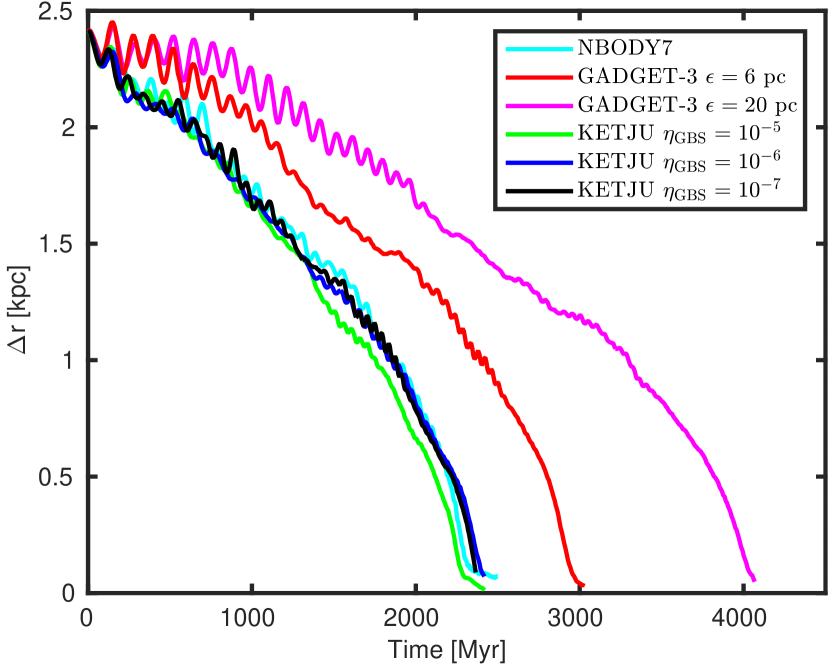
Figure 3.— The separation from the center of the galaxy as a function of simulation time demonstrating the sinking of a SMBH towards the center of a Hernquist sphere using three different numerical codes: NBODY7, GADGET-3 and the KETJU. All three displayed KETJU simulation runs with different GBS integrator accuracies match the SMBH sinking time scale in NBODY7 within a few percent, whereas the GADGET-3 run overpredicts the decay time by a factor of 1.25 to 1.7, depending on the chosen gravitational softening length.

For the GADGET-3 runs, we test two different gravitational softening lengths: $\epsilon=6$ pc and $\epsilon=20$ pc. We set the GADGET-3 integrator error tolerance to $\eta=0.02$ and the force accuracy to $\alpha=0.005$, using the standard GADGET-3 cell opening criterion (Springel, 2005), in all dynamical friction runs. We also run several simulations with higher values for the accuracy parameters obtaining consistently similar results as with the standard parameter values. In the GADGET-3 run with $\epsilon=20$ pc the SMBH reaches the center of the Hernquist sphere on a sinking timescale of $t_{\mathrm{sink}}\sim 4000$ Myr, whereas for the run with $\epsilon=6$ pc the sinking time is $t_{\mathrm{sink}}\sim 3000$ Myr. For both runs the sinking timescales are considerably longer than the sinking timescale in the NBODY7 simulation ($t_{\mathrm{sink}}\sim 2400$ Myr). This is due to the fact that the dynamical friction force is weaker for softened gravitational interactions than for the non-softened forces (Just et al., 2011), as in NBODY7. In simulation codes using gravitational softening, the dynamical friction force contribution of the stars with an impact parameter smaller than the gravitational softening length is grossly underestimated. This results in reduced dynamical friction and affects the sinking timescale of the SMBH although the friction force depends only logarithmically through the Coulomb factor on the impact parameter of the encounters of the SMBH and stellar particles (Binney & Tremaine, 2008).

Including a regularized region around the SMBH overcomes the limitations of the softened tree codes in the computation of the dynamical friction force. In KETJU, the far-field gravitational dynamics of GADGET-3 remains unaltered while the regularized AR-CHAIN integrator handles the close encounters between the SMBH and the incoming stars. We set the gravitational softening length to $\epsilon=6$ pc and the chain radius of the SMBH to be constant at $r_{\mathrm{chain}}=30$ pc ($\lambda=30$, see Eq. (2)). The two important numerical parameters that need to be calibrated are the tidal parameter $\gamma$ and the Gragg-Bulirsch-Stoer (GBS) extrapolation accuracy parameter $\eta_{\mathrm{GBS}}$(see §3.1). The tidal parameter $\gamma$ defines the size of the perturber volume around the regularized subsystem according to Eq. (5). The GBS accuracy parameter $\eta_{\mathrm{GBS}}$ sets the maximum allowed error during a single AR-CHAIN step for any physical variable (see Press et al., 2007, for an in-depth description of the GBS accuracy parameter).

We run the dynamical friction test using KETJU with three different GBS accuracy parameters $\eta_{\mathrm{GBS}}$ $\in[10^{-5},10^{-6},10^{-7}]$. We set the tidal parameter $\gamma$ so that the perturber radius equals twice the radius of the chain subsystem, i.e. 60 pc, which yields good results for all the dynamical friction test runs. During the first $\sim 1.5$ Gyr, the SMBH propagates through the low-density outer parts of the Hernquist sphere and the chain regularization is needed only occasionally when a stellar particle passes very close to the sinking SMBH. After $t>2$ Gyr the regularized subsystem contains particles at every global GADGET-3 timestep. We obtain final SMBH sinking times that are within $4\%$ of the NBODY7 result of $t_{\mathrm{sink}}=2.4$ Gyr using GBS parameter values of $\eta_{\mathrm{GBS}}$ $\leq 10^{-5}$.

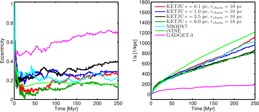
Figure 4.— The evolution of a SMBH binary simulated using NBODY7, standard GADGET-3, rVINE and four KETJU runs. In all KETJU simulations the GBS error tolerance is set to $\eta_{\mathrm{GBS}}$$=10^{-6}$. Left panel: the binary eccentricities are in general small, except for the GADGET-3 run. Right panel: the evolution of the inverse semi-major axis. When the gravitational softening is very small ($\epsilon\lesssim 1$ pc), the KETJU result is close to the NBODY7 result. When $\epsilon$ is increased to $3-5$ pc, the KETJU results appear to converge to a slightly gentler hardening slope than seen in the NBODY7 run. Runs with KETJU and NBODY7 for a low resolution Hernquist sphere with $N=10^{5}$ particles results in unphysically strong two-body relaxationand steep hardening slopes, when $\epsilon\rightarrow 0$. In the GADGET-3 run, the SMBH binary stalls around $1/a\sim 1/\epsilon$, as expected.

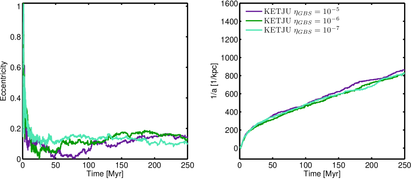
Figure 5.— The effect of the KETJU GBS error tolerance parameter on the SMBH binary evolution. The gravitational softening length is fixed to $\epsilon=6$ pc and the chain radius is set to $r_{\mathrm{chain}}=18$ pc. The run with $\eta_{\mathrm{GBS}}$$=10^{-6}$ is the same as in Fig. 4. All KETJU runs with different $\eta_{\mathrm{GBS}}$ values, $\eta_{\mathrm{GBS}}$$=10^{-5}$, $\eta_{\mathrm{GBS}}$$=10^{-6}$ and $\eta_{\mathrm{GBS}}$$=10^{-7}$, yield consistently similar results both in the evolution of binary eccentricity and the semi-major axis.

4.2. A SMBH binary hardening in a Hernquist sphere

Another crucial feature for a regularized tree code is the ability to properly model the formation and the hardening of systems of binary (or multiple) SMBHs. We build the initial conditions for a SMBH binary hardening test using the same Hernquist spheres as in the previous section. We note that the simulation particle number $N=10^{5}$, limited by the scalability of NBODY7, might be too low to properly study the SMBH binary evolution. Recent state-of-the-art direct summation studies (e.g. Khan et al. 2013; Vasiliev et al. 2014) utilizing $\phi$GRAPE-based codes (Harfst et al., 2007, 2008) have employed particle numbers up to $N\sim 10^{6}$, but as demonstrated by Vasiliev et al. (2015) and Gualandris et al. (2016) even simulations with these high particle numbers are affected by spurious relaxation effects. Instead, our main goal here is to demonstrate that KETJU can reproduce NBODY7 results in simulation setups which are possible to run using NBODY7 in a reasonable wallclock time.

One SMBH with mass of $M_{\bullet}=5\times 10^{7}$ $M_{\odot}$ is placed at rest at the center of the Hernquist sphere while another SMBH of the same mass is placed on a circular orbit with an initial separation of $r=0.1$ kpc from the center of the sphere. We run the simulation for $t=250$ Myr after which the separation of the two SMBHs is $\sim 1$ pc. In the simulation runs using GADGET-3 we set the gravitational softening length of the SMBHs and stellar particles to $\epsilon=10$ pc. The parameter study of KETJU is twofold. First, we set the GBS tolerance to $\eta_{\mathrm{GBS}}$$=10^{-6}$ and test the effect of the gravitational softening length and the chain radius on the SMBH binary evolution. We try four different softening lengths: $\epsilon=0.1$ pc, $\epsilon=1.0$ pc, $\epsilon=3.5$ pc and $\epsilon=6.0$ pc. The chain radius is fixed at $r_{\mathrm{chain}}=10$ pc in the former three runs and set to $r_{\mathrm{chain}}=18$ pc in the last run with the largest softening length. The perturber radius is twice the chain radius in all the simulation runs. The results of this test are presented in Fig. 4.

In the GADGET-3 run the SMBH binary stalls at a separation of $\sim\epsilon$, as expected. In addition, the binary eccentricity is higher in the GADGET-3 run when compared to the rVINE, NBODY7 and KETJU simulations. In rVINE the evolution of the inverse semi-major axis depends on the initial chain radius (Karl et al., 2015). With $N=10^{5}$ stellar particles, the final SMBH binary inverse semi-major axis is somewhat larger in the rVINE run than in the NBODY7 simulation run. As expected, the KETJU runs with the smallest softening lengths match best the evolution of the inverse semi-major axis in NBODY7. With the two larger softening lengths ($\epsilon=3.5$ pc and $\epsilon=6$ pc) the hardening rate appears to converge to a slightly lower value than in the NBODY7 run.

As the host galaxy is a low-resolution Hernquist sphere, the dominating loss-cone filling effect is two-body relaxation. Increasing the gravitational softening length reduces the loss-cone filling rate by increasing the two-body relaxation timescale. Thus it is natural that the hardening rate decreases when the softening length is increased. In a typical real spherical galaxy the two-body relaxation timescale is very long because the number of stars is $N\gg 10^{5}$ and thus the resulting loss-cone filling would be very inefficient, with the hardening rate going towards zero as $N$ increases. However, typically real SMBH binaries form in the aftermaths of galaxy mergers, where the non-spherical shape of the host galaxy is the primary driver for the loss-cone filling instead of two-body relaxation (e.g. Khan et al. 2011). Thus, we here argue that the small differences between the KETJU hardening rates and the NBODY7 results are not a problem when simulating more physical SMBH binary formation scenarios, such as the major mergers of galaxies.

The second part of the KETJU SMBH binary parameter study consists of varying the GBS error tolerance parameter. The gravitational softening was set to $\epsilon=6$ pc and the chain radius to $r_{\mathrm{chain}}=18$ pc for these runs. We tested three different tolerance parameter values: $\eta_{\mathrm{GBS}}$$=10^{-5}$, $\eta_{\mathrm{GBS}}$$=10^{-6}$ and $\eta_{\mathrm{GBS}}$$=10^{-7}$. The results presented in Fig. 5 show that the evolution of both the binary eccentricities and the inverse of the semi-major axis are quite similar for the three runs. In general the orbital eccentricities of the SMBH binaries are quite low $(e<0.4)$ in all the test runs. We do not see any apparent convergence of the results. However, this is not unexpected, as the eccentricity evolution of the SMBH binary is strongly dependent on the velocity distribution of the stellar component (Mikkola & Valtonen, 1992), with the large scatter in the eccentricity just highlighting the low mass resolution of this set of simulations.

In conclusion, all the tested KETJU parameter combinations provide a significantly better description of the SMBH binary dynamics than standard GADGET-3, for which the SMBH binary separation is constrained by the gravitational softening length. KETJU also accurately reproduces the results of NBODY7. Based on these test simulations, we choose the GBS accuracy parameter of $\eta_{\mathrm{GBS}}$$=10^{-6}$ for the rest of the KETJU simulations in this study.

5. Performance and scalability

5.1. Conservation of energy

The earlier FORTRAN-based implementation of the standalone AR-CHAIN algorithm has been demonstrated to conserve energy extremely accurately in few-body ($N_{\mathrm{c}}<10$) simulations (Mikkola & Merritt, 2008). Here we adopt the same test scenario for our C-based AR-CHAIN reimplementation. We set a single SMBH with $M_{\bullet}=10^{10}M_{\odot}$ at rest at the origin. Next, seven stellar particles logarithmically evenly spaced in their mass ratio are drawn from the mass ratio range of $10^{-9}\leq m_{\star}/M_{\bullet}\leq 10^{-3}$ and are placed around the SMBH with a zero initial velocity, resulting in almost rectilinear stellar orbits. We follow the dynamical evolution of the system for 25 000 years. The energy conservation of the system is presented in Fig. 6. The relative energy error remains $|\Delta E/E|=|(H+B)/B|\lesssim 10^{-13}$ for most of the simulation time, where $H$ is the Hamiltonian, which corresponds to the negative of the gravitational binding energy $-B$ in the AR-CHAIN implementation within numerical precision (see Appendix A.).

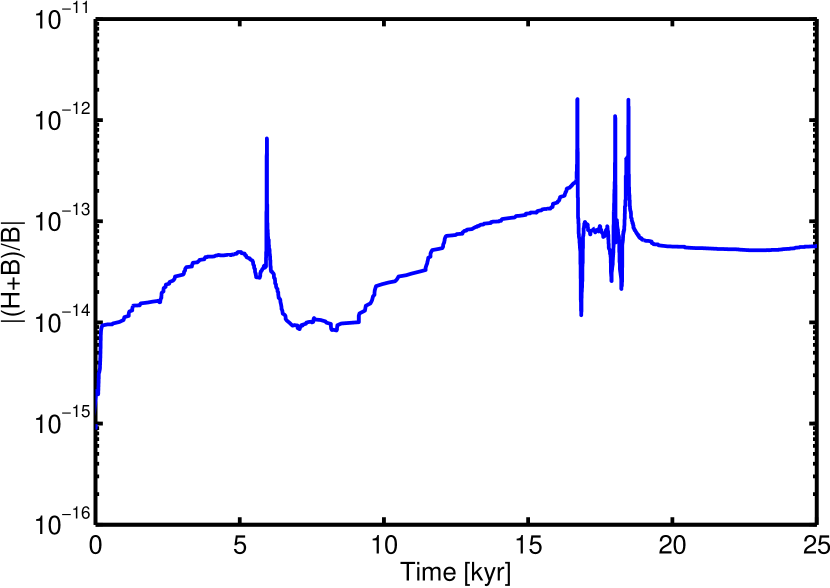
Figure 6.— The relative error of our AR-CHAIN implementation in the extreme accuracy test of Mikkola & Merritt (2008). Here $B$ is the binding energy of the system and $H$ is the Hamiltonian. The relative energy error remains below $10^{-13}$ for most of the simulation time, excluding the most close-by encounters, which are clearly seen as visible jumps in the energy error.

Conservation of energy has to be carefully ensured in KETJU as the gravitational potential in the simulation volume contains both softened and non-softened regions. The energy conservation in the standard softened TreePM algorithm of GADGET-3 was validated by Springel (2005). A simulation particle crossing the boundary from a softened potential to a non-softened regularized region (or vice versa) experiences a sudden discontinuity in the gravitational potential. We next demonstrate that the flux of simulation particles through a chain subsystem does not introduce additional error to the global energy conservation of the simulation.

We set up an energy conservation test by constructing a Hernquist sphere as described in §6 with $M=10^{11}M_{\odot}$ and $N=10^{6}$ particles centered at the origin. A SMBH with $M_{\bullet}=10^{8}M_{\odot}$ is placed at rest at the center of the sphere. The gravitational softening length of stellar particles is set to $\epsilon=6$ pc, the chain radius to 18 pc and the perturber radius to twice the chain radius, i.e. 36 pc. We run the initial conditions for 100 Myr and study the energy conservation as a function of the GBS accuracy parameter. The relative error of the total energy $\left|\Delta E/E_{\mathrm{0}}\right|$ as a function of time is presented in Fig. 7.

We find that energy is conserved in standard GADGET-3 at the level of $\left|\Delta E/E_{\mathrm{0}}\right|\lesssim 1\times 10^{-3}$ during the simulation. KETJU performs sligthly better: $\left|\Delta E/E_{\mathrm{0}}\right|\lesssim 7\times 10^{-4}$ with both $\eta_{\mathrm{GBS}}$$=10^{-6}$ and $\eta_{\mathrm{GBS}}$$=10^{-7}$. The difference between GADGET-3 and KETJU clearly originates from the central tens of parsecs of the galaxy where the accelerations of the simulation particles are the strongest. As KETJU uses the GBS extrapolation method in AR-CHAIN, the energy conservation up to a user-given tolerance is guaranteed in the regularized region during every timestep. In contrast, this is not the case with GADGET-3’s leapfrog integrator: even though the timestepping is adaptive, there is no set maximum allowed energy error per timestep.

Our results can also be compared to the energy conservation of the rVINE code, for which Karl et al. (2015) obtained an energy conservation of $5\times 10^{-4}\lesssim\left|\Delta E/E_{\mathrm{0}}\right|\lesssim 5\times 10^{-3}$ with an initial chain radius of 10 pc in short test runs with a duration of 4.7 Myr and $N=10^{5}$ particles. The exact result depends on the chosen rVINE tree accuracy parameter, but the energy conservation values given above are representative. In both the KETJU test runs shown in Fig. 7, the energy is conserved at a level below $\left|\Delta E/E_{\mathrm{0}}\right|\lesssim 8\times 10^{-5}$ during the first 5 Myr of the simulation. Based on our energy conservation tests, we conclude that KETJU conserves energy on a slightly better level than both standard GADGET-3 and the rVINE code.

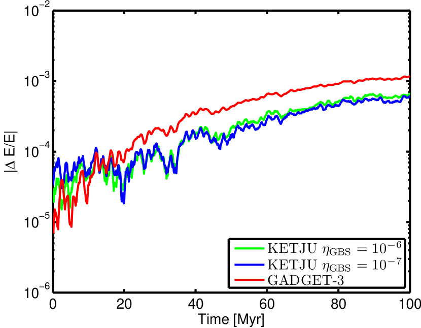
Figure 7.— The relative energy error in GADGET-3 and KETJU in a 100 Myr simulation of an isolated stellar bulge with a single SMBH. The energy conservation is slightly better in all the KETJU runs, when compared to standard GADGET-3.

5.2. Timing tests and code scalability

In this section we demonstrate the scalability of the KETJU code for realistic simulation setups. The performance and scalability of collisionless standard GADGET-3 simulations is presented in Springel et al. (2005). The most time-consuming operations of the GADGET-3 code in simulations without gas are the computation of the gravitational force using the tree algorithm as well as the domain decomposition required for efficient simulation parallelization.

KETJU introduces new computational tasks that need to be performed in addition to the standard GADGET-3 procedures. The most important tasks from the perspective of CPU time consumption are the following: first, the gravitational oct-tree has to be built during every smallest timestep. This is necessary as the chain structure needs to be updated every timestep due to the possibilities of absorption of particles into the chain and the escape of particles from the chain. In addition, the required neighbor searches for chain particles and perturber particles and the resulting extra MPI (Message Passing Interface) communication typically consumes of the order of a few percent of the total CPU time.

Our implementation of the AR-CHAIN algorithm is MPI-parallelized for increased performance and compability with GADGET-3. The KETJU functions are implemented in GADGET-3 in the same manner as all the other subresolution procedures: all MPI tasks participate in a single subresolution routine at a time. The order of the most important AR-CHAIN function calls in the integration cycle of GADGET-3 is briefly discussed at the end of §2.3. Every task contains a copy of the chain structure enabling fast chain-tree particle exhange calculations. Each computational node performs the parallelized chain integration. This computation strategy is found to be faster than the parallelized chain integration using all the available tasks, or serial chain integration and communication of the results to all the tasks. Early development versions of KETJU used all the available MPI tasks for the chain integration, but this proved to be an extremely poor computational strategy when the number of chain particles was far below the number of MPI tasks.

The AR-CHAIN integration of chain particles is the computationally most demanding new operation introduced in KETJU compared to GADGET-3. Estimating the scaling of the computational demand with increasing chain and perturber particle numbers $N_{\mathrm{c}}$ and $N_{\mathrm{p}}$ is not straightforward, since the AR-CHAIN integrator controls both the timestep and the order of the method as necessary to stay within the set accuracy parameters. However, an estimate can be formulated as follows. The amount of required computational work per one force calculation is of the order $\mathcal{O}(N_{\mathrm{c}}^{2}+N_{\mathrm{c}}N_{\mathrm{p}})=\mathcal{O}(\tilde{N}^{2})$, where $\tilde{N}=\sqrt{N_{\mathrm{c}}^{2}+N_{\mathrm{c}}N_{\mathrm{p}}}$ is now an effective number of chain particles. As one force calculation is needed per timestep for a second order leapfrog, the first estimate for the asymptotic computational scaling is just $\mathcal{O}(\tilde{N}^{2})$.

Setting a tolerance limit on the error does not change this in the first approximation. The error $\Delta x$ over one step in some dynamical variable $x$ for a method of order $p$ is $\Delta x\propto h^{p+1}$, where $h$ is the timestep. As such, the global error over a run of time $T$ is $E_{x}\propto Th^{-1}\Delta x\propto h^{p}$. If we set an error tolerance $\epsilon$ and demand $E_{x}\lesssim\epsilon$, we find that $E_{x}\propto T^{1-1/p}\epsilon^{1/p}$ which is independent of the particle number and gives a scaling $\mathcal{O}(\tilde{N}^{2})$ again, if $p$ is constant.

However, the force computation for each particle also suffers from errors accumulated for all the other particles, leading to a force error $\Delta F\propto\tilde{N}^{2}$, which then gives a total error for $x$ of $E_{x}\propto\tilde{N}^{2}h^{p}$. If we then demand $E_{x}\lesssim\epsilon$, we find that $h\propto\epsilon^{1/p}\tilde{N}^{-2/p}$, resulting in a total computational effort of $\propto T\epsilon^{-1/p}\tilde{N}^{2+2/p}$. Thus, the AR-CHAIN algorithm scales as $\mathcal{O}(\tilde{N}^{2+2/p})$, where $p$ is now some mean order used by the GBS extrapolation scheme during the run and which will depend on the smoothness of the problem. In general we have $p\geq 2$, and in the worst case scenario of a simple leapfrog, $p=2$, we have $\mathcal{O}(\tilde{N}^{3})$ scaling. Typically the GBS method works at $p=10$ to $p=16$ which give approximately $\mathcal{O}(\tilde{N}^{2.20})$ and $\mathcal{O}(\tilde{N}^{2.13})$, respectively. As such, we can estimate that the AR-CHAIN integration should scale approximately slightly worse than the square of the particle number.

We perform two scaling tests to study the performance of KETJU. The first scaling test T1 is run using a constant number of MPI tasks while modifying the number of particles in the initial conditions. In the second scaling test T2 the test problem remains fixed but the number of MPI tasks is varied. For both of these test setups we use galaxy merger initial conditions containing two multi-component galaxy models with a stellar bulge, a dark matter halo and a central SMBH. For a detailed description of the initial setup, see §6.1 and Tables 2 and 3. We set the chain radius to 18 pc $(\lambda=1.8$, $\gamma=25)$ in all the scaling test runs. The DM softening length is set to $\epsilon_{\mathrm{DM}}=100$ pc, and the stellar softening length is $\epsilon_{\star}=6$ pc. The number of dark matter particles remains fixed at $N_{\mathrm{DM}}=10^{6}$ in all the scaling test runs. For the scaling tests T1, we select the following accuracy parameters: the GADGET-3 error tolerance $\eta$ $=0.002$ and the AR-CHAIN GBS tolerance of $\eta_{\mathrm{GBS}}=10^{-6}$. We use 96 MPI tasks in all the runs for test sample T1. The number of stellar particles is varied between $2\times 10^{5}\leq N\leq 2\times 10^{6.25}$. The results of the scaling test T1 are presented in Fig. 8.

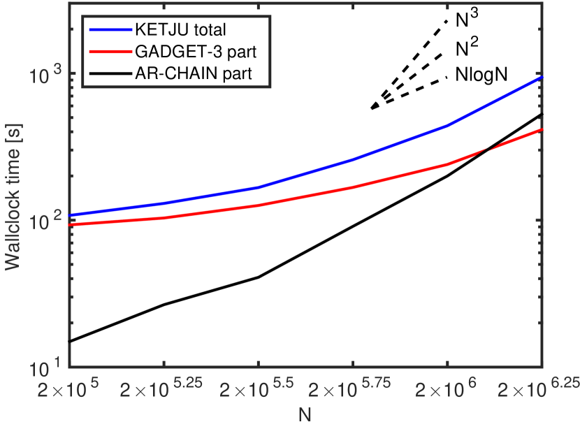
Figure 8.— The scaling test T1. At low particle numbers, the GADGET-3 part dominates the time consumption of KETJU and the scaling is close to the characteristic $\mathcal{O}(N\log{N})$ scaling of GADGET-3. At $N\gg 10^{6}$ the AR-CHAIN part dominates and the scaling is steeper. The maximum stellar particle number which can be run using the current version of KETJU within reasonable wallclock time is $N\sim 5\times 10^{6}$.

When the total number of particles is $N<5\times 10^{5}$, the time consumption of AR-CHAIN is negligible. As ordinary GADGET-3 scales as $\mathcal{O}(N\log{N})$ and the scaling of AR-CHAIN is steeper ($\sim\mathcal{O}(\tilde{N}^{2})$), the wallclock time consumed by the chain computation will eventually exceed the time consumed by the GADGET-3 part. This fact sets the limit on how large particle numbers KETJU can handle: it is not meaningful to run simulations in which the subsystem computations take most of the wallclock time. With the initial condition used here, the AR-CHAIN part takes approximatively half of the computation time for $N\sim 2.5\times 10^{6}$ simulation particles.

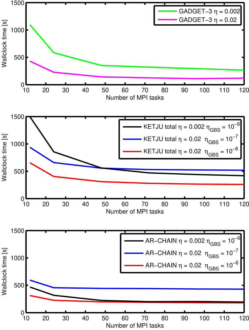
Figure 9.— The scaling test T2: the performance of KETJU and GADGET-3 with different numbers of MPI tasks and different accuracy parameters. Top panel: the scaling for standard GADGET-3. In this particular test the code scales well up to $\sim 50-75$ tasks after which the scaling is poor. Middle panel: the scaling of KETJU is very similar to standard GADGET-3, but KETJU consumes approximatively 50 % more computational time. Bottom panel: the scaling of the AR-CHAIN part is approximately flat, as expected. For more information about the node-based computation strategy, see the text.

In the second scaling test T2, we test the scaling of KETJU as a function of the number of MPI tasks. The number of stellar particles is fixed to $N=2\times 10^{6}$. The results are shown in Fig. 9. We conclude that KETJU scales in a similar manner to standard GADGET-3: the scaling is good up to $\sim 50-75$ MPI tasks after which it is considerably worse. The value of the GBS accuracy parameter $\eta_{\mathrm{GBS}}$ has a large effect on the AR-CHAIN computational time. With $\eta_{\mathrm{GBS}}$ $=10^{-6}$ the chain integration is performed $\sim 2.2$ times faster than when using $\eta_{\mathrm{GBS}}$$=10^{-7}$ with negligible differences in the results as can be seen in §4. With the accuracy parameters in use in §6 ($\eta=0.002$, $\eta_{\mathrm{GBS}}$$=10^{-6}$) KETJU consumes roughly 50 % more computational time than the standard GADGET-3.

From the scalability and timing tests we conclude that the KETJU code is a fast energy-conserving regularized tree code suitable for simulations with up to $N\sim 5\times 10^{6}$ stellar particles in its current configuration. This is sufficient for our current purposes of simulating regularized isolated galaxies and galaxy mergers with SMBHs. We leave further code optimization, required for simulations with particle numbers in excess of $N>5\times 10^{6}$, for future work. We also stress that our code improves on the maximum particle numbers used in the field of studying regularized SMBH dynamics in a galactic environment as current state-of-the-art NBODY simulations typically reach up to $5\times 10^{5}$ - $10^{6}$ simulation particles (see e.g. Wang et al. 2015 and Khan et al. 2011), roughly a factor of $5-10$ below our highest resolution runs presented in §6.

6. Results

Numerical simulations of merging galaxies using direct summation codes with particle numbers of $N\leq 10^{6}$ have recently begun to establish a consensus that the final-parsec problem is in fact nonexistent in galaxy mergers (Khan et al., 2011; Preto et al., 2011). The main conclusion of these studies, that the SMBH hardening rate is in fact resolution-independent in galaxy mergers, was based on the fact that two-body relaxation is not driving the SMBH loss cone refilling. Instead, the non-spherical shape of the galaxy potential provides an additional torque on the stellar orbits, which fill the loss cone on a timescale much shorter than the two-body relaxation timescale. The hardening rate is also large enough to drive the binary to the gravitational wave dominated regime on a timescale that is short compared to the Hubble time.

In this section we use KETJU to study the resolution-dependence of the SMBH binary hardening rates and the timescales of the supermassive black hole mergers using two different types of initial conditions. The first type consists of a stellar bulge and a SMBH without a dark matter halo, a setup which has been extensively used in previous SMBH hardening rate studies (e.g. Khan et al. 2011; Preto et al. 2011). In the second type of initial conditions we include a dark matter halo in addition to the stellar bulge and the SMBH components. The SMBH hardening rates in these more realistic multi-component models have not thus far been rigorously studied in the literature.

6.1. Multi-component equilibrium initial conditions

The initial conditions are generated here using the distribution function method (see e.g. Merritt 1985 and Ciotti & Pellegrini 1992). We model a typical massive elliptical galaxy as an isotropic, spherically symmetric multi-component Hernquist sphere consisting of three components: a stellar component, a dark matter halo and a central SMBH. For a single mass component $i$ the Hernquist density profile with mass $M_{i}$ and scale radius $a_{i}$ is defined as

$$\rho_{i}(r)=\frac{M_{i}}{2\pi}\frac{a_{i}}{r\left(r+a_{i}\right)^{3}},$$ (27)

which corresponds to the simple softened gravitational potential

$$\Phi_{i}(r)=-\frac{GM_{i}}{r+a_{i}}$$ (28)

and the cumulative mass profile

$$M_{i}(r)=M_{i}\frac{r^{2}}{\left(r+a_{i}\right)^{2}}.$$ (29)

The total multi-component potential $\Phi_{\mathrm{T}}$ is the sum of the stellar, dark matter and central SMBH potentials, and is parametrized in our implementation as

$$\Phi_{\mathrm{T}}=\Phi_{\star}+\Phi_{\mathrm{DM}}+\Phi_{\bullet}$$ (30)

$$=-\frac{GM_{\star}}{r+a_{\star}}-\frac{GM_{\mathrm{DM}}}{r+a_{\mathrm{DM}}}-\frac{GM_{\bullet}}{r+\xi_{\bullet}}$$

$$=-GM_{\star}\left[\frac{1}{r+a_{\star}}+\frac{\mu}{r+\beta a_{\star}}+\frac{\eta}{r+\xi_{\bullet}}\right],$$

where the multi-component model parameters are defined as $\mu=M_{\mathrm{DM}}/M_{\star}$, $\eta=M_{\bullet}/M_{\star}$ and $\beta=a_{\mathrm{DM}}/a_{\star}$. This formulation extends the two-component parametrization of Hilz et al. (2012) with the addition of the central SMBH parameters. For numerical reasons, the SMBH potential is softened with a small gravitational softening length of $\xi_{\bullet}$ in order to ensure that the total potential remains finite at $r=0$. We set $\xi_{\bullet}=1\times 10^{-5}$ kpc. Note that $\xi_{\bullet}$ should not be confused with the gravitational softening length of the SMBH in the tree code.

The velocity profiles for the stellar and DM components are obtained using their respective phase-space distribution functions $f_{i}$. This approach has the advantage that it results in more stable initial conditions than using Jeans equations (Binney & Tremaine, 2008; Kazantzidis et al., 2004). In general, the distribution function $f_{i}$ of a density component $\rho_{i}$ in the total gravitational potential $\Phi_{\mathrm{T}}$ is computed using Eddington’s formula (Binney & Tremaine, 2008):

$$f_{i}\left(\mathcal{E}\right)=\frac{1}{\sqrt{8}\pi^{2}}\int_{\Phi_{\mathrm{T}}=0}^{\Phi_{\mathrm{T}}=\mathcal{E}}\frac{d^{2}\rho_{i}}{d\Phi_{\mathrm{T}}^{2}}\frac{d\Phi_{\mathrm{T}}}{\sqrt{\mathcal{E}-\Phi_{\mathrm{T}}}},$$ (31)

in which $\mathcal{E}=-\frac{1}{2}v^{2}-\Phi_{\mathrm{T}}+\Phi_{0}$ is the (positive) energy relative to the chosen zero point of the potential $\Phi_{0}$. In general, the zero point is chosen so that $f_{i}>0$ for $\mathcal{E}>0$ and $f_{i}=0$ for $\mathcal{E}\leq 0$. For an isolated system extending to infinity, such as the Hernquist sphere, we set $\Phi_{0}=0$. Unfortunately, the term $\rho_{i}(\Phi_{\mathrm{T}})$ does not have an analytical expression in the general case. Therefore we rewrite the derivative term of Eq. (31) using the chain rule, following Hilz et al. (2012):

$$\frac{d^{2}\rho_{i}}{d\Phi_{\mathrm{T}}^{2}}=\left(\frac{d\Phi_{\mathrm{T}}}{dr}\right)^{-2}\left[\frac{d^{2}\rho_{i}}{dr^{2}}-\left(\frac{d\Phi_{\mathrm{T}}}{dr}\right)^{-1}\frac{d^{2}\Phi_{\mathrm{T}}}{dr^{2}}\frac{d\rho_{i}}{dr}\right].$$ (32)

The second term of the integral in Eq. (31) is simply

$$\frac{d\Phi_{\mathrm{T}}}{\sqrt{\mathcal{E}-\Phi_{\mathrm{T}}}}=\frac{d\Phi_{\mathrm{T}}}{dr}\frac{dr}{\sqrt{\mathcal{E}-\Phi_{\mathrm{T}}}}.$$ (33)

The resulting expressions contain only first and second derivatives of the density $\rho_{i}$ and the total potential $\Phi_{\mathrm{T}}$ with respect to $r$, which are easily obtained by taking the derivatives of their analytical formulas. Using $r$ as the integration variable naturally changes the limits of the integration. $\Phi_{\mathrm{T}}(r)=\mathcal{E}$ has to be inverted numerically for $r$, whereas the lower integration limit $\Phi_{\mathrm{T}}(r)=0$ corresponds to $r=\infty$.

We compute a random realization of a multi-component Hernquist sphere using the following procedure. First, we draw the random particle positions for the stellar and dark matter components using the inverse cumulative mass profile from Eq. (29). Next, we compute the values of the distribution functions $f_{\star}(\mathcal{E})$ and $f_{\mathrm{DM}}(\mathcal{E})$ into a lookup table using Eqs. (31) and (32). After this we sample the random particle velocities in a computationally efficient way by interpolating the tabulated values of the distribution functions. Finally, we place a SMBH at rest at the center of the multi-component sphere.

We also note here that our initial conditions assume no gravitational softening. Taking the non-zero gravitational softening length into account would result in even more stable initial conditions. Initial conditions that compensate for the gravitational softening have been introduced by e.g. Muzzio (2005) and Barnes (2012). However, in KETJU, the innermost region of the galaxy potential around the central SMBH within the chain radius $r_{\mathbf{chain}}$ is not softened while the rest of the potential is. Consequently, implementing the softening correction in the IC generation may not be completely straightforward and is left as a topic for future code development.

6.2. Galaxy models

We use two principal types of galaxy models in this study: two-component models that in addition to the SMBH only include a stellar bulge (B sample) and three-component models that include a DM halo in addition to the stellar bulge and the central SMBH (H sample). For the stellar bulge component, we set $M_{\star}=10^{11}M_{\odot}$ and $a_{\star}=1.5$ kpc, motivated by the observations of van der Wel et al. (2014) of the mass-size relation of $z\sim 1$ massive early-type galaxies. For the multi-component models including a DM halo, we set, following Hilz et al. (2012), $\beta=11$ and $\mu=100$ motivated by the halo abundance matching results of Moster et al. (2013) yielding $M_{\mathrm{DM}}=10^{13}M_{\odot}$ and $a_{\mathrm{DM}}=16.5$ kpc for the dark matter component. The mass of the central SMBH is set to $M_{\bullet}=10^{8}M_{\odot}$ resulting in $\eta=M_{\bullet}/M_{\star}=0.001$, see Table 2. The motivation for setting up these two simulations samples was to study the hardening rate of the black hole binary in a purely baroynic setting (B sample) and in a setting with a high dark matter fraction (H sample). In this way our two simulation samples bracket the environments found in the centers of typical elliptical galaxies.

The stability of a three-component model with particle numbers ($N_{\mathrm{DM}}=10^{6}$, $N_{\star}=10^{7}$, a single central SMBH) is studied according to the stability test of Hilz et al. (2012) using the standard GADGET-3 code with a gravitational softening length of $\epsilon=20$ pc. The results of the stability test are presented in Fig. 10. The radii containing 10%, 30%, 50% and 80% of the total dark matter mass remain within 1% of their original values during the entire simulation timespan of $t=250$ Myr which corresponds roughly to $\sim 80$ dynamical time scales at the radius enclosing $10$ % of the total stellar mass. The 10% stellar mass radii increases by $\sim 3$ % during the simulation, whereas the other stellar mass radii show even less variation, thus validating the stability of our three-component initial conditions.

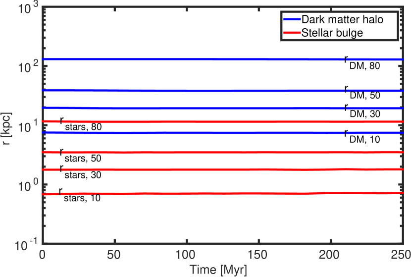
Figure 10.— The stability of the mass radii of an isolated three-component galaxy. The smallest stellar mass radius, $r_{10}$, enclosing the innermost 10% of the stellar mass increases by $\sim 3$% during the run. Other stellar and DM radii remain even more stable.

The two-body relaxation time scale $t_{\mathrm{relax}}$ is defined as

$$t_{\mathrm{relax}}\approx\frac{0.1N}{\ln{N}}\times t_{\mathrm{cross}},$$ (34)

where $N$ is the number of particles and $t_{\mathrm{cross}}$ is the crossing time (Binney & Tremaine, 2008). As the number of stars $(N\sim 10^{11})$ in a massive elliptical galaxy still exceeds the particle number in modern galactic-scale numerical simulations by several orders of magnitude, the simulated galaxies are subject to spurious two-body relaxation effects in their very dense central regions (e.g. Diemand et al. 2004), if no or very small gravitational softening is used. This usually results in a core-like structure in the central region, even without a SMBH, as stars are scattered to lower binding energies (Hilz et al., 2012).

6.3. Galaxy mergers with SMBHs

Table 2Properties of merger progenitor galaxies

Simulation sample	$M_{\star}[10^{10}M_{\odot}]$	$\mu$	$\eta$	$a_{\star}$ [kpc]	$\beta$
B	$10^{11}$	-	$0.001$	1.5	-
H	$10^{11}$	$100$	$0.001$	1.5	11

We set up a sample of 57 major galaxy mergers using the progenitors described in the previous section and in Table 2. The simulation sample is run using KETJU in order to study the dependence of the SMBH binary hardening and the eccentricity evolution on the adopted stellar mass resolution. First, we focus on the binary hardening phase dominated by three-body interactions with the surrounding stars, where the semi-major axis of the binary $a$ lies within $0.1$ pc $\lesssim a\lesssim 5\ \rm pc$ and the Post-Newtonian corrections can be safely neglected. In §6.6 we run a sample of high-resolution simulations including Post-Newtonian corrections until the SMBHs coalesce. A total number of 26 major mergers are run with initial conditions resembling the ones used in the earlier studies of Khan et al. (2011) and Preto et al. (2011): colliding massive stellar bulges without a dark matter halo (sample B in Table 3). The rest of the simulations have a multi-component initial setup: the stellar bulges reside in massive dark matter halos (sample H in Table 3). The particle numbers in different simulations are also presented in Table 3 and range from $2\times 10^{5}$ stellar particles (simulations B1 & H1) to the maximum particle number used in this study: $2\times 10^{6}$ DM particles and $2\times 10^{6.25}\approx 3.6\times 10^{6}$ stellar particles in the merger remnant (simulations B6 & H6). The different simulations within each set for a given resolution only differ in the random seed used in setting up the initial conditions. All simulation samples except for the sample H5 PN are fully Newtonian.

Table 3Particle numbers in the merger remnants

Sample label	$N_{\star}$	$N_{\mathrm{DM}}$	Number of runs with
			different random seeds
B1	$2\times 10^{5}$	-	5
B2	$2\times 10^{5.25}$	-	5
B3	$2\times 10^{5.5}$	-	5
B4	$2\times 10^{5.75}$	-	5
B5	$2\times 10^{6}$	-	5
B6	$2\times 10^{6.25}$	-	1
H1	$2\times 10^{5}$	$2\times 10^{6}$	5
H2	$2\times 10^{5.25}$	$2\times 10^{6}$	5
H3	$2\times 10^{5.5}$	$2\times 10^{6}$	5
H4	$2\times 10^{5.75}$	$2\times 10^{6}$	5
H5	$2\times 10^{6}$	$2\times 10^{6}$	5
H6	$2\times 10^{6.25}$	$2\times 10^{6}$	1
H5 PN	$2\times 10^{6}$	$2\times 10^{6}$	5

The bulge-only galaxies in runs B1-B6 are set on the merger orbit in the following way. The initial separation is chosen to be $d=20\times a_{\star}=30$ kpc. The encounter orbits are nearly parabolic as motivated by cosmological simulations (Khochfar & Burkert, 2006) with the initial velocities chosen as such that the separation of the galactic nuclei is approximately the scale radius $a_{\star}$ during the first pericenter passage. The initial velocities of the galaxies in the H sample (H1-H6) are defined in a slightly different manner. For these mergers, we only consider the mass inside $d=30$ kpc when computing the initial velocities of the galaxies on the parabolic orbit. This results in a slightly faster coalescence of the galactic nuclei in the H sample runs compared to B sample runs. The chain radius is set to $18\ \rm pc$ in all the simulation runs by choosing chain parameters $\lambda=1.8$ and $\gamma=25$. For all runs the gravitational softening lengths are set to $\epsilon_{\star}=6$ pc and $\epsilon_{\mathrm{DM}}=100$ pc for the stellar and dark matter components, respectively. In order to ensure the accuracy of the code with small gravitational softening lengths, we also set the GADGET-3 integrator error tolerance parameter to $\eta=0.002$, which is smaller than the canonical GADGET-3 parameter value by a factor of $\sim 10$. We also tested the chosen set of code parameters for potential pathological simulation behavior. Several runs with slightly different softening lengths, chain radii and error tolerance parameters were performed with similar results compared to the runs with our chosen standard code parameters.

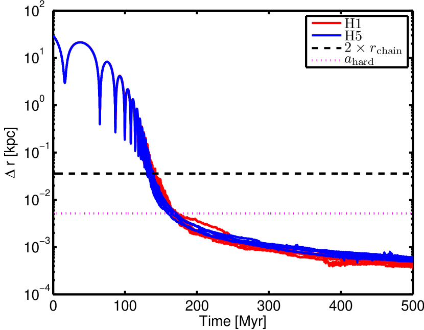
Figure 11.— The smoothed SMBH separation in the simulation runs H1 and H5. The SMBHs form a bound binary at $t\sim 134$ Myr. At this stage the respective stellar cusps of the SMBHs are disrupted and the subsequent hardening of the binary orbit proceeds through three-body interactions. The dashed line marks the radial separation after which the SMBHs belong to the same chain subsystem. The dotted line depicts the the semi-major axis of a hard SMBH binary, as decribed in the main text.

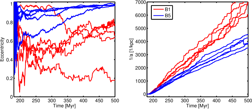
Figure 12.— Binary evolution in the bulge-only simulation sample B. The lines with the same color have the same mass resolution but different random seeds in their initial conditions.

Left panel: the eccentricity evolution after the binary formation. The binary eccentricity is clearly higher and more converged in the high-resolution runs. Right panel: the inverse semi-major axis. The hardening rate $d(1/a)/dt$ decreases when going from low to high resolutions, as expected.

6.4. SMBH binary evolution in merging galaxies

We run all the merger simulations for $t=500$ Myr. The SMBHs lie within the central cusps of their host galaxies for several close passages of the galactic nuclei during the merger until the cusps merge and are quickly disrupted by the formation of the SMBH binary. This occurs at $t\sim 134$ Myr in sample H and at $t\sim 184$ Myr in simulation sample B due to the different encounter orbits of the galaxies with and without the DM halo. After the disruption of the stellar cusps, the dynamical friction becomes inefficient and the binary subsequently hardens via three-body interactions with the surrounding stars. The binary becomes hard when its semi-major axis satisfies the criterion $a<a_{\mathrm{hard}}$. We adopt the definition used by Merritt & Wang (2005) and Merritt et al. (2007): for an equal-mass SMBH binary $a_{\mathrm{hard}}=r_{\mathrm{infl}}/16$, in which the influence radius $r_{\mathrm{infl}}$ is the radius enclosing stellar mass $M_{\star}(r_{\mathrm{infl}})=2M_{\bullet}$. With this definition, $a_{\mathrm{hard}}\sim 5$ pc all the runs. The other commonly used definition for a hard binary is $a_{\mathrm{hard}}=G\mu/4\sigma_{\star}^{2}$, where $\mu$ is the reduced mass of the SMBH binary and $\sigma_{\star}$ is the nuclear stellar velocity dispersion (Merritt, 2006). With this definition $a_{\mathrm{hard}}$ gets slightly lower values. The slingshot-hardening phase continues until the simulation end time at $t=500$ Myr, after which the semi-major axis of the SMBH binary is $0.1$ pc $\lesssim a\lesssim 0.4$ pc $<a_{\mathrm{hard}}$ pc in all the simulation runs. The separation of the two SMBHs as a function of time during the galaxy merger for simulations H1 and H5 is presented in Fig. 11.

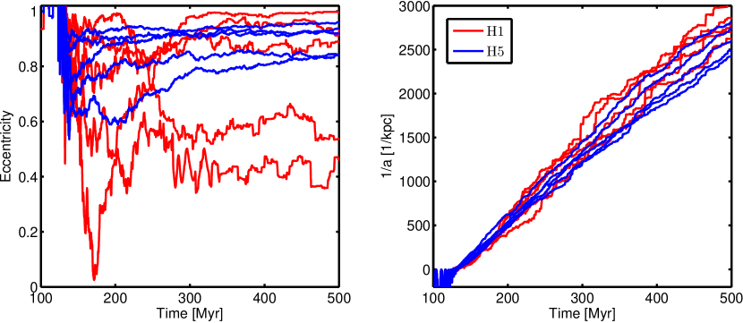
Figure 13.— The evolution of the binary in the halo-included simulation sample H. The lines with the same color have the same mass resolution but different random seeds in their initial conditions. The binary eccentricities are quantitatively similar in simulation samples B and H. However, in contrast to simulation sample B the evolution of the hardening rate $d(1/a)/dt$ of the inverse semi-major axis for sample H shows no apparent resolution-dependence.

We show the evolution of the orbital eccentricity and the inverse semi-major axis of the SMBH binaries of sample B1 and B5 in Fig. 12 and H1 and H5 in Fig. 13. The binary eccentricities in the high-resolution simulations B5 and H5 are in general high, $0.6<e<1.0$ with most of the binaries having eccentricities in excess of $e>0.8$. At lower resolutions, the stellar field surrounding the binary is resolved less accurately resulting in lower binary eccentricities and a significantly larger scatter between different runs with different initial random seeds. This is expected since the eccentricity evolution of the binary, especially at the moment of the binary formation, depends sensitively on the velocity field of the surrounding stars (Mikkola & Valtonen, 1992). The eccentricity of the SMBH binary also increases due to the exchange of angular momentum with the surrounding stars. Typically, the SMBH binary eccentricity increases during the slingshot-hardening phase if it is high enough to begin with. However, the eccentricity growth rate decreases for binaries with initially low eccentricities $(e<0.5)$ and is $\sim 0$ for circular binaries (Sesana et al., 2006). This situation may be different in stellar systems that are strongly corotating with the SMBH binary (Sesana et al., 2011) as the binary circularizes instead of becoming more eccentric.

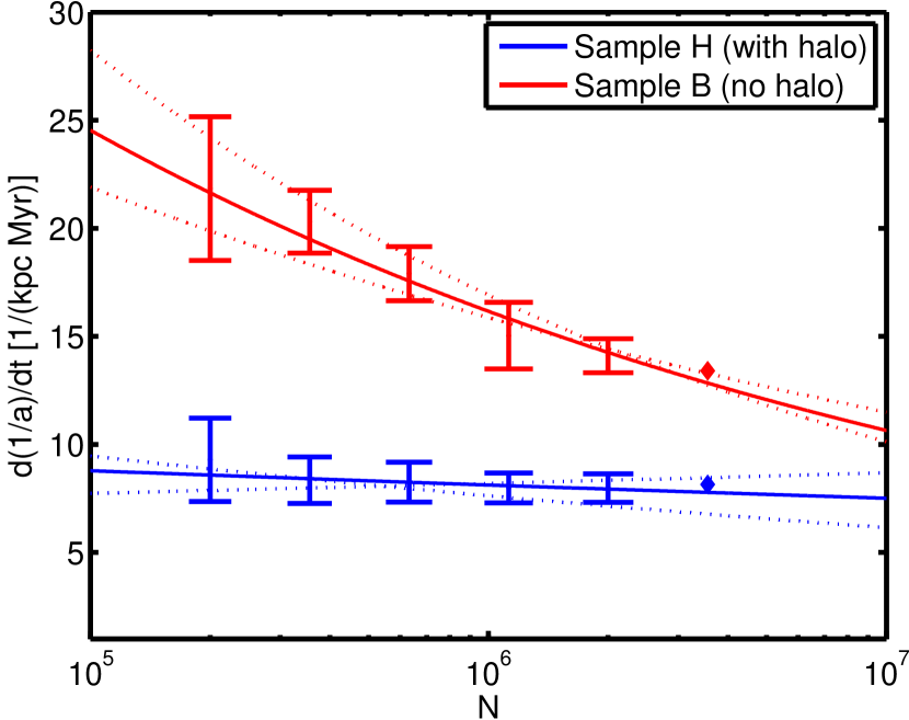
Figure 14.— The SMBH binary hardening rates as function of the simulation stellar particle number, represented with error bars of 1 standard deviation. The bulge-only simulations show a dependence on the particle number, $\propto N^{-0.18\pm 0.04}$. If the DM halo is included, the power-law $\propto N^{-0.03\pm 0.06}$ is consistent with no resolution-dependence in the H sample, as described in the text. The three fits for each sample are plotted with the mean power-law exponent and the mean exponent $\pm$ error of one standard deviation.

The evolution of the inverse semi-major axis is very close to linear ($1/a\propto t$) during the hardening phase in all the runs of simulation samples B and H until $t=500$ Myr. The binary hardening rates are presented in Fig. 14 as a function of the stellar particle number of the merger remnant. The mean hardening rates with errors of one standard deviation from the selected samples are as follows: B1: $21.8\pm 3.3$ kpc^-1Myr^-1, B5: $14.1\pm 0.8$ kpc^-1Myr^-1, H1: $9.3\pm 1.9$ kpc^-1 Myr^-1 and H5: $8.0\pm 0.7$ kpc^-1Myr^-1. We further quantify the resolution dependence of the hardening rates by fitting a power-law $d(1/a)/dt\propto N^{-\alpha}$ to the results and studying the distribution of the power-law exponent $\alpha$. This is done by using a simple bootstrap method. Considering first sample B, we pick a random run from each subsample B1-B6 each and fit the power-law. We repeat this procedure $10^{4}$ times and obtain the mean $\alpha$ and its standard deviation. The process is then repeated for sample H. In sample B, the hardening rate clearly depends on the stellar mass resolution:

$$\frac{\mathrm{d}}{\mathrm{d}t}\left(\frac{1}{a}\right)_{\mathrm{B}}\propto N^{-0.18\pm 0.04},$$ (35)

whereas, sample H is consistent with no resolution dependence of the hardening rate:

$$\frac{\mathrm{d}}{\mathrm{d}t}\left(\frac{1}{a}\right)_{\mathrm{H}}\propto N^{-0.03\pm 0.06}.$$ (36)

The resolution-dependence of the hardening rate originates from the resolution-dependence of the process which fills the loss cone of the SMBH binary. If the shape of the merger remnant is sufficiently asymmetric, the stellar orbits are torqued into the loss cone of the SMBH binary at a rate higher than the loss cone filling produced by the resolution-dependent two-body relaxation. Consequently, the resolution-dependence of the SMBH binary hardening rate decreases (Merritt & Poon, 2004; Berczik et al., 2006; Khan et al., 2011). We next study the shapes of the merger remnants in samples B and H. In calculating the shapes of the merger remnants we closely follow the S1 method of Zemp et al. (2011). The axis ratios $b/a$ and $c/a$ are computed in thin ellipsoidal shells from the eigenvalues of the shape tensor of the stellar matter distribution. We note that the axis ratios of the merger remnants remain roughly constant after the nuclei of the progenitor galaxies have merged. The axis ratios for the simulation samples B1, B5, H1 and H5 are presented in Fig. 15 as a function of the distance from the center of the galaxy.

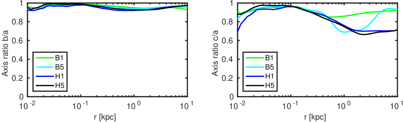
Figure 15.— The host galaxy axis ratios $b/a$ and $c/a$ in merger samples B5 and H5 as a function of radius. Left panel: the ratio $b/a$ is high, $\sim 0.95$, in all simulation samples B1, B5, H1 and H5. Right panel: the axis ratio $c/a$. The axis ratios are similar for samples H1 and H5, $c/a\sim 0.7$ at $r>1$ kpc, with $c/a$ close to unity inside this radius. However, the $c/a$ values for B1 and B5 clearly differ from each other and the H sample simulations, see text for further details.

All the merger remnants are roughly axisymmetric: $b/a\sim 0.9$ for all the simulation samples between $10^{-2}$ kpc $\leq r\leq 10$ kpc. The $c/a$ ratio is roughly $0.8$ near the SMBH binary and $\sim 0.95$ at $r=0.1$ kpc for all the simulation samples. However, at larger radii the differences between the samples become evident. For samples H1 and H5 the $c/a$ ratio decreases outwards and is $\sim 0.7$ at $r=10$ kpc. For the sample B1 $0.8<c/a<0.9$ in the outer parts of the galaxy, whereas simulation sample B5 contains a flatter region with $c/a\sim 0.7$ between $0.5$ kpc $\lesssim r\lesssim 5$ kpc. We attribute this phenomenon to the fact that relaxation effects are stronger in low-resolution simulations (e.g. Power et al. 2003), and the flatter feature has relaxed away in the B1 lower resolution runs. The stellar orbits are defined by the total potential $\Phi_{\mathrm{T}}$. If the massive DM halo is present, the potential of the galaxy $\Phi_{\mathrm{T}}$ is dominated by the collisionless halo component $\Phi_{\mathrm{DM}}$ and the relaxation-induced evolution of the stellar component $\Phi_{\star}$ has only a small effect on the total potential $\Phi_{\mathrm{T}}$. Thus, it is natural that the axis ratios of samples H1 and H5 are more similar than for the bulge only B1 and B5 samples.

6.5. Quantifying the differences in the hardening rates

After studying the ellipsoidal axis ratios of the merger remnants, we further quantify the differences of the stellar populations in simulation samples B1, B5 and H5. Both the SMBH binary hardening hardening rates and merger remnant axis ratios in sample H1 are very close to the corresponding quantities of sample H5, thus we left sample H1 out of the analysis. In addition to the loss-cone filling rate, the hardening rate of the SMBH binary also depends on the distribution of the pericenter distances and the velocties of the incoming stars. Three-body scattering experiments have shown that, on average, stars with smaller pericenter distance and smaller initial velocity gain more energy from the binary in the star-binary interaction (see e.g. Valtonen & Karttunen 2006 for a review on this topic.)

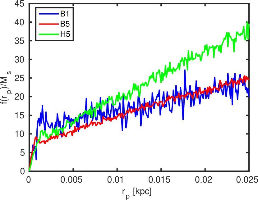
Figure 16.— The distribution of the stellar pericenter distances with respect to the center-of-mass of the SMBH binary during $200$ Myr $<t<400$ Myr. During this period, the semi-major axis of the binary is between $5$ pc and $0.5$ pc in all the simulation runs. The distribution function $f(r_{\mathrm{p}})$ is normalized to the total stellar mass $M_{\mathrm{s}}$ entering a sphere within a radius of $r=30$ pc centered on the center-of-mass of the SMBH binary. In sample B1, a larger fraction of stars have pericenter distances of $r_{\mathrm{p}}<10$ pc compared to sample B5.

We present the distribution of pericenter distances $r_{\mathrm{p}}$ of stellar particles in Fig. 16 during $200$ Myr $<t<400$ Myr. During this period, the semi-major axis $a$ of the binary is between $5$ pc and $0.5$ pc in all the simulation runs. The pericenter distance distribution $f(r_{\mathrm{p}})$ is normalized by the total stellar mass $M_{\mathrm{s}}$ entering a sphere with a radius of $r=30$ pc centered on the binary. The radius of $30$ pc is chosen based on the numerical criterion that stars with pericentric distances of $r_{\mathrm{p}}\lesssim 6\times a$ interact strongly with the binary (Mikkola & Valtonen, 1992). Stars passing the binary with a larger pericenter distance just perturb the binary’s center-of-mass and have a negligible effect on the orbital elements of the binary itself (e.g. Quinlan 1996). In sample H5, more stellar mass enters the vicinity of the SMBH binary compared to the samples B1 and B5. This is due to the fact that the velocity dispersion for the H5 sample is higher than in the B simulation samples because of the presence of the massive DM halo. The additional incoming stars in H5 are distributed towards larger values of $r_{\mathrm{p}}$ compared to B1 and B5. However, a larger number of incoming stars does not make the hardening rates of SMBH binaries in the sample H5 greater, as also the velocities of the stars are higher. Comparing the bulge-only samples B1 and B5 we see that there is more stellar mass at the pericenter distances of $r_{\mathrm{p}}<10$ pc in the low-resolution run. Again, we attribute this phenomenon to spurious relaxation effects due to the low stellar mass resolution in the B1 sample. More stellar mass at low pericenter distances in sample B1 contributes to the higher SMBH binary hardening rate compared to higher resolution sample B5.

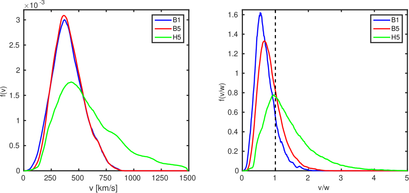
Figure 17.— Left panel: the velocity distribution of stellar particles crossing a shell at a distance $r=30$ pc from the SMBH binary during $200$ Myr $<t<400$ Myr. Because of the deep potential well of the DM halo in H5, there are fewer particles with low velocities and a large number of particles with high velocities $v>750$ km/s compared to the bulge-only samples. The difference between the B1 and B5 samples is the low-velocity tail in the distribution of B1. Right panel: the distribution of stellar particle velocities with respect to the time-dependent watershed velocity $w$, see the text for a definition. Now the difference of samples B1 and B5 becomes clear: there are more particles with velocties below the watershed velocity $w$ in B1 than in B5. These slowly moving stellar particles harden the SMBH binary efficiently.

Next, we study the distribution of the stellar particles which pass closer than $r=30$ pc from the center-of-mass of the binary in merger samples B1, B5 and H5. Here the concept of the so-called watershed velocity $w$ is extremely useful:

$$w\approx 0.85\times\sqrt{\frac{M_{\bullet,1}}{M_{\bullet,1}+M_{\bullet,2}}}V_{\mathrm{bin}}=0.85\times\sqrt{\frac{GM_{\bullet,2}}{a}},$$ (37)

in which $V_{\mathrm{bin}}$ is the orbital velocity of the SMBH binary components (Quinlan, 1996). For an equal-mass SMBH binary, the watershed velocity is $w\approx 0.6\times V_{\mathrm{bin}}$. On average, incoming stars with a velocity $v<w$ gain energy from the binary which then hardens. Likewise, stars with $v>w$ are likely to lose energy to the binary which then becomes wider. This is because for $v<w$, the velocity in the binary orbit is higher than the approach velocity of the incoming star and the star is more easily captured onto a bound orbit. On a bound orbit the star will eventually pass close to either one or both of the SMBHs and is then ejected from the vicinity of the SMBH binary. Faster stars with $v>w$ are less likely to become bound to the binary (Valtonen & Karttunen, 2006). Note that $w$ is obviously time-dependent: if the SMBH binary hardens, $w$ increases. Thus, there are more particles with $v<w$ to efficiently harden the binary. However, this effect is somewhat balanced by the fact that the region of strong three-body interactions ($r<6\times a$) becomes smaller as the SMBH binary hardens.

The velocity distributions $f(v)$ and $f(v/w)$ of the stellar particles crossing a shell at a distance of $30$ pc from the SMBH binary during $200$ Myr $<t<400$ Myr are shown in Fig. 17. The bulge in the H5 sample is situated in a massive DM halo resulting in higher velocities of the incoming stellar particles than in the bulge-only samples. Consequently, the sample H5 has the highest fraction of particles with velocities above the watershed velocity $w$. This is why the hardening rates of the SMBH binaries in the H5 sample are smaller than in samples B1 and B5, even though there is more stellar mass in sample H5 interacting with the binary, as can be seen in Fig. 16.

The velocity distributions $f(v)$ for the bulge-only samples B1 and B5 differ at low velocities: the low-velocity tail for B1 extends to lower velocities than for sample B5. The reason for the differences of the hardening rates between samples B1 and B5 becomes more clear when studying the incoming stellar velocity distribution $f(v/w)$ with respect to the time-dependent watershed velocity $w$. There is a larger fraction of stellar particles with velocities $v<w$ in sample B1 resulting in a higher hardening rate than in sample B5. In addition, there are more particles with small pericenter distances as seen in Fig. 16. We note that the the distribution $f(v/w)$ acts as an exaggerated version of $f(v)$: as there are more low-velocity stellar particles in B1, the SMBH binary hardens faster. Thus, the watershed velocity $w$ increases, and more stellar particles now have $v<w$ even if $f(v)$ remains constant.

To sum up the results: we studied the distributions of pericenter distances and the approach velocities of the stellar particles interacting with the SMBH binary in order to explain why the hardening rates decrease when adding a massive DM halo or when increasing the stellar mass resolution. We find that sample B1 has both the smallest stellar approach velocities with respect to the SMBH binary watershed velocity $w$ and more particles at small pericenter distances from the binary. In the sample B5 there are slightly less particles with small pericenter distances and, more importantly, less particles with low velocities. The halo-including sample H5 has far fewer stellar particles at velocities $v<w$, which explains the lowest hardening rate, even though more stellar mass interacts with the SMBH binary for this simulation sample. We find that this picture is consistent with the study of Gualandris et al. (2016): mergers without a DM halo result in a merger remnant in which the SMBH binary evolution depends on the particle number used when $N<10^{7}$. However, we note that while Khan et al. (2011) and Preto et al. (2011) reported resolution-independent SMBH binary hardening in mergers without a DM halo, we find resolution-independent hardening rates only in the merger simulations, which use multi-component ICs including a DM halo. However, some of the differences might be attributed to the fact that the parameters of the progenitor galaxies and the merger orbits are not exactly the same in the different studies. Probing the full galaxy and merger orbit parameter space would require a far larger simulation sample than the 57 merger runs used in this work and is beyond the scope of the present study.

The hardening rates are also large enough to drive the binaries into the gravitational wave (GW) dominated regime ($a\sim 0.1$ pc for a circular SMBH binary) less than $\sim 1$ Gyr after the formation of the binary. As the binary eccentricities are high, $0.8<e<0.95$ in our highest-resolution simulations with a DM halo, the expected SMBH merger timescale for these simulations is less than a gigayear. We conclude that the final-parsec problem does not exist in our simulation sample of mergers of massive elliptical galaxies. In addition, the incorporation of the massive dark matter halo in the multi-component initial conditions reduces the resolution-dependence of the SMBH binary hardening rates and in practice makes the hardening rate resolution-independent within the range of particle numbers used in this study.

6.6. SMBH merging timescales

We run five additional simulations at the resolution of sample H5 presented in Fig. 13, but this time including also Post-Newtonian corrections in order to obtain the actual merging timescales of the SMBH binaries. This sample is labelled H5 PN. Only the SMBH-SMBH terms in the PN equations of motion are included since the star-SMBH terms would be unphysically large as the stellar particle masses are $m_{\star}\gg M_{\odot}$ in our simulations. We include Post-Newtonian terms up to order PN2.5, the highest of which is the radiation-reaction term. We chose not to include the higher-order terms as there is still some ambiguity in the literature over the derivation of these terms and as the contribution of the next radiation-reaction term at PN3.5 is proportional to $\propto c^{-7}$, its effect would be anyhow negligible (see e.g. Will 2006 for further details).

We run the five simulations until the coalescence of the binaries. The orbital evolution of the binaries is presented in Fig. 18. The binary evolution is qualitatively similar compared to the purely Newtonian case when $a>0.75$ pc - $1$ pc: the binary hardens at a constant rate and becomes slowly more eccentric due to interactions with the surrounding stars. After this point, the GW emission determines the orbital evolution of the SMBH binary up to the final coalescence.

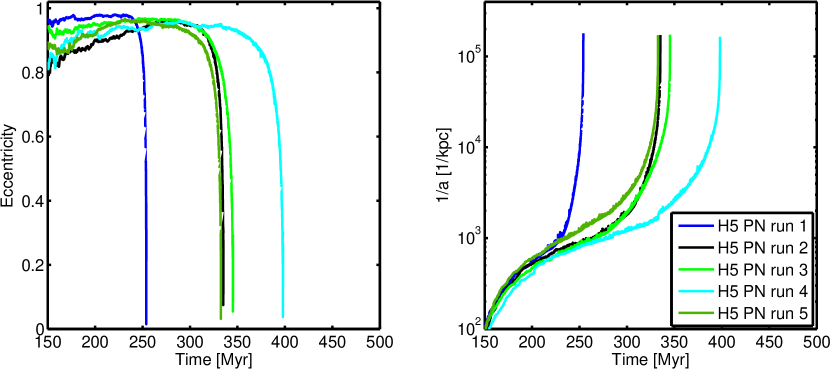
Figure 18.— The Post-Newtonian binary evolution in five runs from the simulation sample H5 PN. As the SMBH binary eccentricities are high, the SMBH mergers occur rapidly, $120$ Myr - $264$ Myr after the formation of the binaries. It is important to note that a scatter of $\Delta e\sim 0.15$ in binary eccentricity results in a large difference $\Delta t\sim 144\ \rm Myr$ in the coalescence times. The large scatter in the SMBH coalescence timescale is due to the very steep dependence of the GW emission on the binary eccentricity.

The radiative losses of binary orbital energy and angular momentum are both extremely sensitive to the eccentricity of the binary. During a single orbital period, the average PN2.5 order loss effects are, according to Peters & Mathews (1963),

$$-\langle\dot{E}\rangle=\frac{32G^{4}M_{\bullet,1}^{2}M_{\bullet,2}^{2}(M_{\bullet,1}+M_{\bullet,2})}{5c^{5}a^{5}}\frac{1+\frac{73}{24}e^{2}+\frac{37}{96}e^{4}}{(1-e^{2})^{7/2}},$$ (38)

$$-\langle\dot{L}\rangle=\frac{32G^{7/2}M_{\bullet,1}^{2}M_{\bullet,2}^{2}\sqrt{M_{\bullet,1}+M_{\bullet,2}}}{5c^{5}a^{7/2}}\frac{1+\frac{7}{8}e^{2}}{(1-e^{2})^{2}},$$ (39)

which both diverge as $e\rightarrow 1$. For example, a binary with $e=0.95$ radiates $\sim 127$ times more GW energy during a single orbital period than a binary with $e=0.8$ assuming equal semi-major axes. For this reason, the initially more eccentric binaries coalesce on much shorter timescales. At $t=150$ Myr, or $16$ Myr after the binary formation, the eccentricities of the binaries are $0.80\lesssim e\lesssim 0.96$. The peak eccentricities reach $e>0.95$ for all the five binaries before the gravitational wave driven circularization phase begins. During the final tens of millions of years before the coalescence, the binary circularizes and hardens very rapidly. Both the orbital decay and circularization of the binary are consistent with Peters’ analytic formulas (Peters & Mathews, 1963). The SMBH coalescences occur at $120$ Myr, $199$ Myr, $201$ Myr, $211$ Myr and $264$ Mr after the binary formation. The difference in the final BH coalescence time can vary up to $\sim 50$% between the mergers, although the simulations were set up with identical initial conditions, with the only difference being in the initial random seed.

The final SMBH separation before the coalescence is $\sim 1000$ AU in all three simulations. This is a significant improvement over the merging criterion typically used in softened GADGET-3-based codes in which the typical SMBH merger separation is of the order of $10$-$100$ pc at the time of the merger (e.g. Springel et al. 2005; Johansson et al. 2009b; Salcido et al. 2016). Obtaining the distribution of the SMBH merger timescales for a representative simulation sample would require substantial further work and is beyond the scope of this study. However, we emphasize that the only difference in the five initial conditions of the presented Post-Newtonian simulations is the random number seed used in our multi-component initial conditions generator. The realized eccentricity scatter of $\Delta e\sim 0.15$ resulted in a difference of $\Delta t\sim 144$ Myr in the SMBH merger timescale.

Based on our three-body experiments we expect that the eccentricity scatter will decrease with an increasing stellar mass resolution. Thus, future work aiming at obtaining accurate SMBH merger timescales should focus on simulating the galaxy merger and the merger remnant in the most accurate manner and with the highest resolution possible, as the binary eccentricity evolution depends sensitively on the stellar velocity field around the binary. This ambitious goal requires going to particle numbers significantly beyond the value of $N_{\star}>3.6\times 10^{6}$ used in the present study.

As the hardening rate of an equal-mass SMBH binary in relatively unsensitive to the eccentricity (Mikkola & Valtonen, 1992; Quinlan, 1996), we can estimate the maximum SMBH coalescence timescale for our galaxy models and SMBH masses used without running additional simulations. The maximum coalescence timescale is obtained in the situation in which the SMBH binary eccentricity remains zero during the entire slingshot-hardening phase and the GW inspiral. The merging timescale can be estimated as follows. Assuming that the hardening rate $s=d(1/a)/dt$ from the three-body interactions is constant and $e=0$, the time $t_{\mathrm{f}}$ from the initial semi-major axis $a_{0}$ to the final value $a_{\mathrm{f}}$ is given by

$$t_{\mathrm{f}}=\int_{a_{\mathrm{f}}}^{a_{0}}\frac{da}{sa^{2}+\mathrm{C}_{\mathrm{PM}}a^{-3}},$$ (40)

which is most conveniently solved numerically. Here $\mathrm{C}_{\mathrm{PM}}$ is the absolute value of the constant appearing in the Peters’ formula (Eq. 12). Setting $a_{\mathrm{f}}=1000$ AU mimicking the SMBH coalescence distance in KETJU and $a_{0}=0.01$ kpc, we get the maximum possible SMBH merging timescales of $\sim 2$ Gyr for the B5 sample and $\sim 3.1$ Gyr for the H5 sample using the hardening rates obtained in §6.4. As mentioned in §6.2, the DM content of galaxy models used in this study brackets the realistic population of elliptical galaxies so the maximum possible SMBH merger timescale is 2-3 Gyr for the used SMBH mass and the initial stellar distribution. The maximum merging timescales are well below the Hubble time, but are long enough that subsequent galaxy mergers may have time to bring in additional SMBHs near the original binary. This usually results in the rapid merging of two of the SMBHs while the third one is dynamically ejected from the center of the galaxy. Finally, we note that the maximum SMBH merging timescales obtained here are very likely to be dependent on the central stellar density profiles of the progenitor galaxies and may thus not be generalized in a straightforward manner.

7. Discussion

The new code developed in this study allows us to simultaneously model accurately both the dynamics close to SMBHs and the global galactic dynamics of their host galaxies. The primary motivation for developing this new code was two-fold. Firstly, we want to push the numerical resolution of the galactic scale simulations ultimately to unprecedented particle numbers $(N\gtrsim 10^{7}-10^{8})$ and secondly, the new code allows for galactic-scale dynamical studies that include also a gaseous component and their associated feedback processes. Both of these goals are difficult to reach with traditional $N$-body codes even allowing for GPU acceleration, as for these codes the particle numbers are typically limited to $N\sim 10^{6}$ and the inclusion of the gaseous component is in general not straightforward to implement (see e.g. Nitadori & Aarseth 2012; Wang et al. 2015, 2016).

As in the hierarchical model galaxies grow through mergers, situations with multiple SMBHs in the merger remnant will be frequently encountered. Recently an increasing number of systems with multiple SMBHs have been detected (e.g. Valtonen et al. 2008; Boroson & Lauer 2009; Deane et al. 2014). However, the absolute number of such systems still remains relatively low, which may indicate that the dynamical friction driven decay of the SMBH orbits and their eventual mergers are relatively rapid processes.

The key prediction to come out of an accurate dynamical simulation is the actual merging timescale of the SMBHs. Often the orbital decay of SMBHs has been studied using either global isolated merger simulations or full cosmological simulations (e.g. Springel et al. 2005; Sijacki et al. 2015), which both have typically employed softened gravity, such as is used in standard GADGET-3. We showed in Fig. 3 the well-known result that softened calculations underestimate the dynamical friction effect of stars with impact parameters smaller than the gravitational softening length, which depending on the situation can result in dynamical friction timescales that are off by a factor of a few. This problem is largely circumvented in direct $N$-body simulations with no or very low gravitational softening, albeit at the cost of the simulation typically starting from rather idealized initial conditions in which the SMBHs are already relatively close, thus often missing the preceding dynamical friction phase altogether (e.g. Berczik et al. 2006; Khan et al. 2011). The KETJU code is an optimal tool in circumventing both of these problems and we have demonstrated in this article that the code can be used to study the orbital decay of SMBHs in a realistic galactic setting.

The dynamical friction phase is followed by first the phase in which the binary hardens through three-body interactions with the stellar background leading ultimately to the gravitational wave driven phase, which is responsible for the final merging of the SMBHs. Typically the softening length is set to $\sim 1-20$ pc in isolated merger simulations (e.g. Hopkins et al. 2013; Choi et al. 2014) and to $\sim 100-500$ pc (e.g. Feldmann et al. 2016; Choi et al. 2016) in high-resolution cosmological simulations, both of which provide insufficient resolution for studying the binary hardening at $1-10\ \rm pc$ spatial scales and the eventual GW driven coalescense at centiparsec scales. The typical solution for this predicament is the adoption of subresolution models for the unresolved dynamics of the system, with the most famous prescription being the original recipe used in Springel et al. (2005), which postulated instantaneous merging of nearby SMBHs, with the resulting merger taking place typically at $\sim 10-100$ pc distances depending somewhat on the exact numerical resolution.

As these subresolution descriptions lead often to very rapid SMBH merging (e.g. Sijacki et al. 2015) the burning question now remains whether this is realistic. The simulations presented in this study show that the final GW phase of the SMBH merger sensitively depends on the eccentricity of the SMBH binary, with eccentricity differences ($e\sim 0.80-0.96$) resulting in coalescense time differences of up to $\Delta t\sim 144\ \rm Myr$ (see Fig. 18). This is readily expected as the energy emitted in gravitational waves very strongly depends on the eccentricity of the SMBH binary (see Eq. (38)). The eccentricities being of paramount importance it is critical that the global evolution of the galaxy merger leading up to the formation of the SMBH binary is modeled accurately, which the KETJU code is able to do as demonstrated in §6.

The SMBH binaries formed during galaxy mergers are also expected to contribute a cosmological background of nanohertz-frequency gravitational waves. However, contrary to this expectation, pulsar timing array measurements during the last few years have to date yielded no sign of the expected gravitational wave background (Shannon et al., 2015; Arzoumanian et al., 2016). The measurements have placed an upper limit of $\sim 1.0\times 10^{-15}$ for the characteristic strain amplitude of the gravitational wave background, measured at the frequency of $f=1\ \rm yr^{-1}$. Currently these upper limits are inconsistent on the $\sim 1-2$ sigma level with recent models of gravitational wave background formation from SMBH binaries in galaxy mergers (e.g. Sesana 2013; McWilliams et al. 2014; Kulier et al. 2015), indicating that current models of SMBH dynamics might overestimate the SMBH merger rates, or that the SMBH masses themselves may be systematically overestimated (e.g. Rasskazov & Merritt 2016; Sesana et al. 2017). Thus it is important to provide more accurate theoretical predictions of the SMBH merger timescales that might help in reconciling the derived upper limits of the pulsar timing array measurements with theory and ultimately pave the way for more accurate predictions required by future space-borne GW detection experiments (e.g. Amaro-Seoane et al. 2012).

We have here demonstrated the functionality of KETJU in collisionless simulations that include SMBHs and both stellar and dark matter particles. However the real future strength of the code lies in realistic galactic-scale simulations that also include a gaseous component. In the KETJU code the AR-CHAIN algorithm solves the stellar dynamics close to the SMBH, whereas all of the astrophysical processes, such as hydrodynamics, cooling, star formation and stellar feedback is performed in the GADGET-3 code using already existing routines (Hu et al., 2014, 2016). Unlike the collisionless stellar component collisional, gas can cool and collapse towards the center of the galaxy, thus shaping the central gravitational potential with potentially interesting consequences for the final-parsec problem (e.g. Lodato et al. 2009). However, special care will be required for the treatment of feedback from the SMBHs, as we can now dynamically probe centiparsec scales for which the standard approach of taking the Bondi-Hoyle accretion rate is destined to fail (e.g. Curtis & Sijacki 2015).

In addition, simulations that accurately obtain the coalescence timescale of binary SMBHs in gas-rich galaxy mergers are also essential for providing accurate estimates for the expected recoil velocities of merged SMBHs and the likelihood that the recoiling SMBHs escape the deepening central gravitational potential (e.g. Blecha et al. 2011, 2016). The recoil probability will be particularly relevant for large-scale cosmological simulations such as Illustris and EAGLE (Vogelsberger et al., 2014; Schaye et al., 2015) that typically assume rapid coalescense below the spatial resolution limit and which also often fix the SMBHs to the center of the potential using an artificial repositioning scheme (Johansson et al., 2009b). The more accurately predicted coalescense times of SMBHs in cosmological simulations will also directly impact the estimate of the strength of the gravitational wave background. Finally, the accurate dynamical modeling of the SMBHs could shed light on the possible offsets between the central SMBH and the hosting dark matter halo, which will be important for experiments that attempt a direct detection of the possible central dark matter annihilation signal (e.g. Batcheldor et al. 2010; Lacroix et al. 2014). SMBH binaries can also change the stellar dynamics of the nuclear regions of the host galaxy, which can be now probed with integral field unit (IFU) observations (Thomas et al., 2016).

8. Conclusions

In this article we present and test the performance of KETJU, a new regularized tree code based on algorithmic chain regularization (AR-CHAIN integrator) implemented into GADGET-3 (Springel, 2005). The key feature of the KETJU code is the inclusion of regularized regions around every SMBH, which allows for the accurate simultaneous modeling of the global dynamics on galactic scales together with the sub-parsec-scale SMBH evolution. The code also includes Post-Newtonian corrections up to order PN3.5, which also includes the PN2.5 term responsible for gravitational wave emission. This allows us in principle to follow the evolution of the SMBH binary down to spatial scales of $\sim 10$ Schwarzschild radii, which is an improvement of several orders of magnitude over the merger separations traditionally employed in softened GADGET-3-based codes ($\sim 10-100\ \rm pc$, e.g. Springel et al. 2005; Johansson et al. 2009b; Salcido et al. 2016). The more accurate treatment of all three phases (dynamical friction, three-body interactions and GW emission) relevant for SMBH merging in one global simulation provides improved constraints on the SMBH coalescense timescales in galaxy mergers with potentially important implications for future gravitational wave experiments, such as LISA (e.g. Amaro-Seoane et al. 2007).

The KETJU code was calibrated against NBODY7 (Aarseth, 2012) by running test simulations. In the first simulation we followed the inspiral of a single SMBH in a Hernquist sphere, whereas in the second simulation we studied the hardening of a SMBH binary system inside another Hernquist sphere. In both tests we were able to reproduce the results of NBODY7 at high accuracy thus validating the performance of the AR-CHAIN integrator and the KETJU code. In addition the energy conservation was demonstrated to be on a good level both for the stand-alone AR-CHAIN integrator and the KETJU code, which performed slightly better than the standard GADGET-3 code. The scaling of the KETJU code was adequate up to $\sim 75$ processors. We conclude that this is an area which will require substantial future improvement, if the ultimate goal of simulating up to $N\sim 10^{7}-10^{8}$ particles is to be reached.

We used the KETJU code to study the resolution dependence of the SMBH binary hardening rates and the SMBH coalescense timescales in a set of galaxy mergers. We extend the initial conditions of the progenitor galaxies to include in addition to the stellar bulge and SMBH, also a dark matter halo component motivated by the studies of Hilz et al. (2012). We run a total of 57 merger simulations with particle numbers reaching up to $2\times 10^{6}$ DM particles and $2\times 10^{6.25}\approx 3.6\times 10^{6}$ stellar particles for the highest resolution simulations. Half of the simulations included only a bulge component in addition to the SMBH, whereas the other half also included a dark matter component. We found a mild dependence of the SMBH binary hardening rate on the mass resolution of the simulation in the simulations without a DM halo. The time evolution of the inverse semi-major axis of the binary orbit was proportional to particle number $N$ as $d(1/a)/dt\propto N^{-0.18\pm 0.04}$ for the mergers without a DM halo. In the halo-including sample we found $d(1/a)/dt\propto N^{-0.03\pm 0.06}$, which is consistent with no resolution-dependence. We thus see a weaker dependence on numerical resolution for the simulation sample that includes a massive DM halo. We did not encounter the final-parsec problem in any of our merger simulations. This result is attributed to the non-spherical structure of the merger remnants. The non-spherical shape of the merger remnant torques the stellar orbits to fill the SMBH binary loss cone faster than the two-body relaxation, which is artificially boosted by the low mass resolution (e.g. Berczik et al. 2006). We find that this result is in good agreement with the previous work of Gualandris et al. (2016).

The shapes of the stellar components of the merger remnants are very similar in all simulations including the DM component. We attribute this to the fact that the massive halo dominates the galactic potential and thus relaxation effects in the stellar component are less important. This results in similar distributions of pericenter distances and approach velocities for the stars interacting with the SMBH binary, and consequently to nearly similar SMBH binary hardening rates at all resolutions. In the bulge-only mergers the differences in the merger remnant shapes are larger (see Fig. 14) as the relaxation effects are more important in the absence of the massive DM halo. In low-resolution bulge-only simulations, there are more stellar particles with low velocities and small pericenter distances compared to the high-resolution bulge-only simulations. This explains the resolution-dependence of hardening rates for the bulge-only simulation sample. In addition, the SMBH binary hardening rates are higher in bulge-only simulations compared to the hardening rates of simulations that include a massive DM halo, due to the higher stellar velocities in these galaxies. The eccentricities of the SMBH binaries formed in the merger remnants are in general very high ($e\sim 0.9$), which is a direct consequence of the initial orbits of the progenitor galaxies. However, we see a scatter in the eccentricity of $\Delta e\sim 0.15$ for simulation setups that only differ in the random seed used to generate the multi-component initial conditions. The scatter in eccentricity produced essentially by stochastic encounters between the SMBH and stellar particles (Mikkola & Valtonen, 1992) can result in considerable differences in the SMBH coalescence timescales of the order of $\sim 140\ \rm Myr$ due to the steep scaling of gravitational wave emission with the binary eccentricity (see Eq. (38)).

Development of hybrid regularized tree codes that allow the simultaneous modeling of the global dynamics on galactic scales together with the sub-parsec-scale SMBH evolution will hopefully help to bridge the gap between the galaxy formation and $N$-body communities. We find the KETJU code is an important step in this direction, but we end by stressing that the particle and the stellar mass resolutions significantly beyond the ones employed in this study are still required for obtaining truly highly accurate predictions for the timescales of SMBH mergers.

Appendix A Appendix A: Algorithmic regularization

We start with the usual Newtonian N-body Hamiltonian

$$H=\sum_{i}\frac{1}{2}m_{i}\|\boldsymbol{v}_{i}\|^{2}-\sum_{i}\sum_{j>i}\frac{Gm_{i}m_{j}}{\|\boldsymbol{r}_{ij}\|}=T-U,$$ (A1)

where $m_{i}$ are the masses, $\boldsymbol{v}_{i}$ velocities and $\boldsymbol{r}_{ij}=\boldsymbol{r}_{j}-\boldsymbol{r}_{i}$ relative separations of the N bodies, $T$ is the total kinetic energy and $U$ is the force function, or equivalently the negative of the Newtonian potential energy. The binding energy of the system is $B=-H=U-T$. This Hamiltonian generates the usual N-body equations of motion

$$\dot{\boldsymbol{r}}_{i} =\boldsymbol{v}_{i}$$ (A2)

$$\dot{\boldsymbol{v}}_{i} =\sum_{j\neq i}\frac{Gm_{j}\boldsymbol{r}_{ij}}{\|\boldsymbol{r}_{ij}\|^{3}}.$$ (A3)

This system is transformed by introducing a new fictitious time, or independent variable, $s$ with the definitions

$$\mathrm{d}s=\left[\alpha(T+B)+\beta\omega+\gamma\right]\mathrm{d}t=\left[\alpha U+\beta\Omega+\gamma\right]\mathrm{d}t,$$ (A4)

where $\alpha$, $\beta$ and $\gamma$ are real constants, $\Omega(\{\boldsymbol{r}_{i}\})$ is in principle an arbitrary real-valued function of the coordinates, and $\omega$ is a new velocity-like variable, for which we define

$$\dot{\omega}=\sum_{i}\boldsymbol{\nabla}_{\boldsymbol{r}_{i}}\Omega\cdot\boldsymbol{v}_{i}$$ (A5)

and $\omega(0)=\Omega(\{\boldsymbol{r}_{i}(0)\})$. Following Mikkola & Merritt (2006, 2008) we set

$$\Omega=\sum_{i<j}\frac{\Omega_{ij}}{\|\boldsymbol{r}_{ij}\|},$$ (A6)

where $\Omega_{ij}=\tilde{m}^{2}$ if $m_{i}m_{j}<\epsilon_{\Omega}\tilde{m}^{2}$ and $\Omega_{ij}=0$ otherwise. Here

$$\tilde{m}^{2}=\frac{2}{N(N-1)}\sum_{i<j}m_{i}m_{j},$$ (A7)

is the mean product of particle masses, with $N$ equal to the number of particles. Following Mikkola & Merritt (2008), we set the parameter $\epsilon_{\Omega}=10^{-3}$. This choice of $\Omega$ is made to guarantee that low-mass particles have a non-negligible effect on the regularization, even though they make only a negligible contribution to the value of $U$.

With these definitions, the two definitions in Eq. (A4) are equivalent on the exact integral curve, since $T+B=U$ and $\Omega(\{\boldsymbol{r}_{i}(t)\})=\omega(t)$. With prime signifying a derivative with respect to $s$, we get the following equations of motion for the coordinates,

$$t^{\prime} =\left[\alpha(T+B)+\beta\omega+\gamma\right]^{-1}$$ (A8)

$$\boldsymbol{r}^{\prime}_{i} =t^{\prime}\boldsymbol{v}_{i}$$ (A9)

and for the velocities

$$t^{\prime} =\left(\alpha U+\beta\Omega+\gamma\right)^{-1}$$ (A10)

$$\omega^{\prime} =t^{\prime}\sum_{i}\boldsymbol{\nabla}_{\boldsymbol{r}_{i}}\Omega\cdot\boldsymbol{v}_{i}$$ (A11)

$$\boldsymbol{v}^{\prime}_{i} =t^{\prime}\sum_{j\neq i}\frac{Gm_{j}\boldsymbol{r}_{ij}}{\|\boldsymbol{r}_{ij}\|^{3}}.$$ (A12)

In the presence of perturbing accelerations $\boldsymbol{f}_{i}$, the binding energy of the system will not be constant, but instead

$$\dot{B}=-\dot{T}+\dot{U}=-\sum_{i}m_{i}\boldsymbol{v}_{i}\cdot\boldsymbol{f}_{i},$$ (A13)

since the Keplerian accelerations cancel. With this addition the time transformed velocity equations read

$$t^{\prime} =\left(\alpha U+\beta\Omega+\gamma\right)^{-1}$$ (A14)

$$B^{\prime} =-t^{\prime}\sum_{i}m_{i}\boldsymbol{v}_{i}\cdot\boldsymbol{f}_{i}$$ (A15)

$$\omega^{\prime} =t^{\prime}\sum_{i}\boldsymbol{\nabla}_{\boldsymbol{r}_{i}}\Omega\cdot\boldsymbol{v}_{i}$$ (A16)

$$\boldsymbol{v}^{\prime}_{i} =t^{\prime}\left(\sum_{j\neq i}\frac{Gm_{j}\boldsymbol{r}_{ij}}{\|\boldsymbol{r}_{ij}\|^{3}}+\boldsymbol{f}_{i}\right).$$ (A17)

Different choices of the parameter triplet $(\alpha,\beta,\gamma)$ correspond to different algorithmic regularization schemes, with $(1,0,0)$ yielding the logarithmic Hamiltonian method (Mikkola & Tanikawa, 1999; Preto & Tremaine, 1999) and $(0,1,0)$ being equivalent to the Time-Transformed Leapfrog scheme (Mikkola & Aarseth, 2002). Both give exact orbits for two-body orbits including collisions. We choose $(\alpha,\beta,\gamma)=(1,0,0)$, based on the suggestion in Mikkola & Merritt (2008). For a more extended discussion of possible parameter choices, see Mikkola & Merritt (2006) and Mikkola & Merritt (2008).

Appendix B Appendix B: Chained leapfrog

When the Eqs. (23) are time transformed as described in Appendix A, we end up with the following equations of motion for the chain coordinates

$$t^{\prime} =\left[\alpha(T+B)+\beta\omega+\gamma\right]^{-1}$$ (B1)

$$\boldsymbol{X}^{\prime}_{i} =t^{\prime}\boldsymbol{V}_{i},$$ (B2)

and the velocities

$$t^{\prime} =\left(\alpha U+\beta\Omega+\gamma\right)^{-1}$$ (B3)

$$B^{\prime} =-t^{\prime}\sum_{i}m_{i}\boldsymbol{v}_{i}\cdot\boldsymbol{f}_{i}$$ (B4)

$$\omega^{\prime} =t^{\prime}\sum_{i}\boldsymbol{\nabla}_{\boldsymbol{X}_{i}}\Omega\cdot\boldsymbol{V}_{i}$$ (B5)

$$\boldsymbol{V}^{\prime}_{i} =t^{\prime}\left(\boldsymbol{A}_{i}(\{\boldsymbol{X}_{i}\})+\boldsymbol{f}_{i}+\boldsymbol{g}_{i}(\boldsymbol{v}_{i})\right)$$ (B6)

$$\boldsymbol{S}^{\prime}_{i} =t^{\prime}\boldsymbol{S}_{\text{PN},i}\times\boldsymbol{S}_{i},$$ (B7)

where $\boldsymbol{g}_{i}(\boldsymbol{v}_{i})$ are the perturbing accelerations which depend on the particle velocities. If the perturbing accelerations do not depend on the particle velocities, that is $\boldsymbol{g}_{i}=0$, the Eqs. (B3)-(B7) can immediately be integrated with a standard leapfrog. In this case, while the equations of motion for $B$ and $\omega$ depend on velocities, the dependence is linear, and as such can be analytically integrated over one timestep. It should be noted that in practice it is easier to evaluate the derivatives of $B$ and $\omega$ using the non-chained velocities $\boldsymbol{v}_{i}$ and coordinates $\boldsymbol{r}_{i}$, but using Eq. (24) for the relative distances $\boldsymbol{r}_{ij}$.

However, it should be noted that the Post–Newtonian corrections (§ 3.2) do depend on the particle velocities, and possibly spins, in addition to the particle coordinates. In this case, the equations of motion (B3)-(B7) are no longer integrable, and normally an implicit method would have to be used to compute the solution over one timestep. This is undesirable, since an implicit method generally requires iterating to convergence, which would force re-evaluating the computationally heavy PN corrections several times. This can be avoided by extending the phase space, which allows an explicit leapfrog to be constructed, as in Hellström & Mikkola (2010) or using the generalization derived in Pihajoki (2015). Combined with the extrapolation method, this allows the PN corrections to be implemented with a much smaller computational overhead.

The phase space extension is done by introducing auxiliary velocities $\boldsymbol{w}_{i}$ and the corresponding auxiliary chained velocities $\boldsymbol{W}_{i}$ as well as auxiliary spins $\boldsymbol{Z}_{i}$ for each particle. An auxiliary time transformation variable $\sigma$ is required as well. Before the leapfrog step, these are set to the values of the original variables. Then, when the velocity kicks are calculated, the value of $\boldsymbol{w}_{i}$ is used to compute $\dot{\boldsymbol{v}}_{i}$, and similarly the value of $\boldsymbol{v}_{i}$ is used to compute $\dot{\boldsymbol{w}}_{i}$. Evolution of the spin and the time transformation variable is done in a similar alternating way.

The end result is a leapfrog, which can be written with mappings $\mathbf{X}(\Delta s)$ (drift) and $\mathbf{V}(\Delta s)$ (kick), which propagate the system in the phase space. We list the algorithmic form of these mappings below. The maps can then be combined to form the two second order leapfrogs commonly called drift-kick-drift (DKD) leapfrog $\mathbf{X}(h/2)\mathbf{V}(h)\mathbf{X}(h/2)$ and the kick-drift-kick (KDK) leapfrog $\mathbf{V}(h/2)\mathbf{X}(h)\mathbf{V}(h/2)$, where $h$ is the timestep. In the code, the DKD leapfrog is used.

procedure $\mathbf{X}$($\Delta s$)

     $T\leftarrow\sum_{i=1}^{N}\frac{1}{2}m_{i}\|\boldsymbol{v}_{i}\|^{2}$

     $\Delta t\leftarrow\Delta s/\left[\alpha(T+B)+\beta\omega+\gamma\right]$

     $t\leftarrow t+\Delta t$

     for $i\leftarrow 1,\ldots,N-1$ do

         $\boldsymbol{X}_{i}\leftarrow\boldsymbol{X}_{i}+\Delta t\,\boldsymbol{V}_{i}$

     end for

end procedure

Algorithm 1 $\mathbf{X}(\Delta s)$

procedure PhysicalStep($\Delta t$)

     Evaluate $\boldsymbol{w}_{i}$ using $\boldsymbol{W}_{i}$, $\boldsymbol{g}_{i}$ using $\boldsymbol{w}_{i}$ and $\boldsymbol{S}_{\text{PN},i}$ using $\boldsymbol{Z}_{i}$

     $\omega\leftarrow\omega+\Delta t\,\sum_{i=1}^{N}\boldsymbol{\nabla}_{\boldsymbol{r}_{i}}\Omega\cdot\boldsymbol{w}_{i}$

     $B\leftarrow B-\Delta t\sum_{i=1}^{N}m_{i}\boldsymbol{w}_{i}\cdot(\boldsymbol{f}_{i}+\boldsymbol{g}_{i})$

     for $i\leftarrow 1,\ldots,N-1$ do

         $\boldsymbol{V}_{i}\leftarrow\boldsymbol{V}_{i}+\Delta t\left(\boldsymbol{F}_{i+1}-\boldsymbol{F}_{i}+\boldsymbol{f}_{i+1}-\boldsymbol{f}_{i}+\boldsymbol{g}_{i+1}-\boldsymbol{g}_{i}\right)$

     end for

     for $i\leftarrow 1,\ldots,N$ do

         $\boldsymbol{S}_{i}\leftarrow\boldsymbol{S}_{i}+\Delta t\,\boldsymbol{S}_{\text{PN},i}\times\boldsymbol{Z}_{i}$

     end for

end procedure

procedure AuxiliaryStep($\Delta t$)

     Evaluate $\boldsymbol{v}_{i}$ using $\boldsymbol{V}_{i}$, $\boldsymbol{g}_{i}$ using $\boldsymbol{v}_{i}$ and $\boldsymbol{S}_{\text{PN},i}$ using $\boldsymbol{S}_{i}$

     $\sigma\leftarrow\sigma+\Delta t\sum_{i=1}^{N}\boldsymbol{\nabla}_{\boldsymbol{r}_{i}}\Omega\cdot\boldsymbol{v}_{i}$

     for $i\leftarrow 1,\ldots,N-1$ do

         $\boldsymbol{W}_{i}\leftarrow\boldsymbol{W}_{i}+\Delta t\left(\boldsymbol{F}_{i+1}-\boldsymbol{F}_{i}+\boldsymbol{f}_{i+1}-\boldsymbol{f}_{i}+\boldsymbol{g}_{i+1}-\boldsymbol{g}_{i}\right)$

     end for

     for $i\leftarrow 1,\ldots,N$ do

         $\boldsymbol{Z}_{i}\leftarrow\boldsymbol{Z}_{i}+\Delta t\,\boldsymbol{S}_{\text{PN},i}\times\boldsymbol{S}_{i}$

     end for

end procedure

procedure $\mathbf{V}$($\Delta s$)

     $U\leftarrow\sum_{i=1}^{N}\sum_{j>i}^{N}\frac{Gm_{i}m_{j}}{r_{ij}}$

     $\Omega\leftarrow\Omega(\boldsymbol{r}_{1},\ldots,\boldsymbol{r}_{N})$

     $\Delta t\leftarrow\Delta s/\left(\alpha U+\beta\Omega+\gamma\right)$

     for $i\leftarrow 1,\ldots,N$ do

         $F_{i}=\sum_{j\neq i}\frac{Gm_{j}\boldsymbol{r}_{ij}}{\|\boldsymbol{r}_{ij}\|^{3}}$

     end for

     Compute velocity independent perturbations $\boldsymbol{f}_{i}$

     AuxiliaryStep$(\Delta t/2)$

     PhysicalStep$(\Delta t)$

     AuxiliaryStep$(\Delta t/2)$

end procedure

Algorithm 2 $\mathbf{V}(\Delta s)$

References

- Aarseth (1999) Aarseth, S. J. 1999, PASP, 111, 1333
- Aarseth (2012) Aarseth, S. J. 2012, MNRAS, 422, 841
- Abbott et al. (2016) Abbott, B. P., et al. 2016, Physical Review Letters, 116, 061102
- Amaro-Seoane et al. (2007) Amaro-Seoane, P., et al. 2007, Classical and Quantum Gravity, 24, R113
- Amaro-Seoane et al. (2012) Amaro-Seoane, P., et al. 2012, Classical and Quantum Gravity, 29, 124016
- Armitage & Natarajan (2005) Armitage, P. J., & Natarajan, P. 2005, ApJ, 634, 921
- Arzoumanian et al. (2016) Arzoumanian, Z., et al. 2016, ApJ, 821, 13
- Barker & O’Connell (1975) Barker, B. M., & O’Connell, R. F. 1975, Phys. Rev. D, 12, 329
- Barnes & Hut (1986) Barnes, J., & Hut, P. 1986, Nature, 324, 446
- Barnes (2012) Barnes, J. E. 2012, MNRAS, 425, 1104
- Batcheldor et al. (2010) Batcheldor, D., Robinson, A., Axon, D. J., Perlman, E. S., & Merritt, D. 2010, ApJ, 717, L6
- Begelman et al. (1980) Begelman, M. C., Blandford, R. D., & Rees, M. J. 1980, Nature, 287, 307
- Berczik et al. (2006) Berczik, P., Merritt, D., Spurzem, R., & Bischof, H.-P. 2006, ApJ, 642, L21
- Binney & Tremaine (2008) Binney, J., & Tremaine, S. 2008, Galactic Dynamics: Second Edition (Princeton University Press)
- Blecha et al. (2011) Blecha, L., Cox, T. J., Loeb, A., & Hernquist, L. 2011, MNRAS, 412, 2154
- Blecha et al. (2016) Blecha, L., et al. 2016, MNRAS, 456, 961
- Booth & Schaye (2009) Booth, C. M., & Schaye, J. 2009, MNRAS, 398, 53
- Boroson & Lauer (2009) Boroson, T. A., & Lauer, T. R. 2009, Nature, 458, 53
- Bulirsch & Stoer (1966) Bulirsch, R., & Stoer, J. 1966, Numerische Mathematik, 8, 1
- Chandrasekhar (1943) Chandrasekhar, S. 1943, ApJ, 97, 255
- Chapon et al. (2013) Chapon, D., Mayer, L., & Teyssier, R. 2013, MNRAS, 429, 3114
- Choi et al. (2014) Choi, E., Naab, T., Ostriker, J. P., Johansson, P. H., & Moster, B. P. 2014, MNRAS, 442, 440
- Choi et al. (2012) Choi, E., Ostriker, J. P., Naab, T., & Johansson, P. H. 2012, ApJ, 754, 125
- Choi et al. (2016) Choi, E., Ostriker, J. P., Naab, T., et al. 2016, ArXiv e-prints, arXiv:1610.09389
- Ciotti & Pellegrini (1992) Ciotti, L., & Pellegrini, S. 1992, MNRAS, 255, 561
- Costa et al. (2014) Costa, T., Sijacki, D., & Haehnelt, M. G. 2014, MNRAS, 444, 2355
- Curtis & Sijacki (2015) Curtis, M., & Sijacki, D. 2015, MNRAS, 454, 3445
- Davis et al. (2013) Davis, T. A., Alatalo, K., et al. 2013, in IAU Symposium, Vol. 295, The Intriguing Life of Massive Galaxies, ed. D. Thomas, A. Pasquali, & I. Ferreras, 324–327
- Deane et al. (2014) Deane, R. P., et al. 2014, Nature, 511, 57
- Dehnen (2014) Dehnen, W. 2014, Computational Astrophysics and Cosmology, 1, 1
- Di Matteo et al. (2005) Di Matteo, T., Springel, V., & Hernquist, L. 2005, Nature, 433, 604
- Diemand et al. (2004) Diemand, J., Moore, B., Stadel, J., & Kazantzidis, S. 2004, MNRAS, 348, 977
- Dubois et al. (2012) Dubois, Y., Devriendt, J., Slyz, A., & Teyssier, R. 2012, MNRAS, 420, 2662
- Einstein et al. (1938) Einstein, A., Infeld, L., & Hoffmann, B. 1938, Annals of Mathematics, 39, 65
- Feldmann et al. (2011) Feldmann, R., Carollo, C. M., & Mayer, L. 2011, ApJ, 736, 88
- Feldmann et al. (2016) Feldmann, R., et al. 2016, ArXiv e-prints, arXiv:1610.02411
- Ferrarese & Ford (2005) Ferrarese, L., & Ford, H. 2005, Space Sci. Rev., 116, 523
- Ferrarese & Merritt (2000) Ferrarese, L., & Merritt, D. 2000, ApJ, 539, L9
- Fujii et al. (2007) Fujii, M., Iwasawa, M., Funato, Y., & Makino, J. 2007, PASJ, 59, 1095
- Gebhardt et al. (2000) Gebhardt, K., et al. 2000, ApJ, 539, L13
- Genzel et al. (2014) Genzel, R., et al. 2014, ApJ, 796, 7
- Gragg (1965) Gragg, W. B. 1965, SIAM Journal on Numerical Analysis, 2, 384
- Gualandris & Merritt (2012) Gualandris, A., & Merritt, D. 2012, ApJ, 744, 74
- Gualandris et al. (2016) Gualandris, A., Read, J. I., Dehnen, W., & Bortolas, E. 2016, MNRAS, arXiv:1609.09383
- Hairer et al. (2008) Hairer, E., Nørsett, S., & Wanner, G. 2008, Solving Ordinary Differential Equations I: Nonstiff Problems, Springer Series in Computational Mathematics (Springer Berlin Heidelberg)
- Harfst et al. (2008) Harfst, S., Gualandris, A., Merritt, D., & Mikkola, S. 2008, MNRAS, 389, 2
- Harfst et al. (2007) Harfst, S., Gualandris, A., Merritt, D., et al. 2007, New Astronomy, 12, 357
- Häring & Rix (2004) Häring, N., & Rix, H.-W. 2004, ApJ, 604, L89
- Hellström & Mikkola (2010) Hellström, C., & Mikkola, S. 2010, Celestial Mechanics and Dynamical Astronomy, 106, 143
- Hernquist (1990) Hernquist, L. 1990, ApJ, 356, 359
- Hills & Fullerton (1980) Hills, J. G., & Fullerton, L. W. 1980, AJ, 85, 1281
- Hilz et al. (2012) Hilz, M., Naab, T., Ostriker, J. P., et al. 2012, MNRAS, 425, 3119
- Holley-Bockelmann & Khan (2015) Holley-Bockelmann, K., & Khan, F. M. 2015, ApJ, 810, 139
- Hopkins et al. (2013) Hopkins, P. F., Cox, T. J., Hernquist, L., et al. 2013, MNRAS, 430, 1901
- Hu et al. (2016) Hu, C.-Y., Naab, T., Walch, S., Glover, S. C. O., & Clark, P. C. 2016, MNRAS, 458, 3528
- Hu et al. (2014) Hu, C.-Y., Naab, T., Walch, S., Moster, B. P., & Oser, L. 2014, MNRAS, 443, 1173
- Iwasawa et al. (2015) Iwasawa, M., Portegies Zwart, S., & Makino, J. 2015, Computational Astrophysics and Cosmology, 2, 6
- Jernigan & Porter (1989) Jernigan, J. G., & Porter, D. H. 1989, ApJS, 71, 871
- Johansson et al. (2009a) Johansson, P. H., Burkert, A., & Naab, T. 2009a, ApJ, 707, L184
- Johansson et al. (2009b) Johansson, P. H., Naab, T., & Burkert, A. 2009b, ApJ, 690, 802
- Johansson et al. (2012) Johansson, P. H., Naab, T., & Ostriker, J. P. 2012, ApJ, 754, 115
- Just et al. (2011) Just, A., Khan, F. M., Berczik, P., Ernst, A., & Spurzem, R. 2011, MNRAS, 411, 653
- Karl et al. (2015) Karl, S. J., Aarseth, S. J., Naab, T., Haehnelt, M. G., & Spurzem, R. 2015, MNRAS, 452, 2337
- Kazantzidis et al. (2004) Kazantzidis, S., Magorrian, J., & Moore, B. 2004, ApJ, 601, 37
- Kelley et al. (2017a) Kelley, L. Z., Blecha, L., & Hernquist, L. 2017a, MNRAS, 464, 3131
- Kelley et al. (2017b) Kelley, L. Z., Blecha, L., Hernquist, L., & Sesana, A. 2017b, ArXiv e-prints, arXiv:1702.02180
- Kesden (2012) Kesden, M. 2012, Phys. Rev. D, 85, 024037
- Khan et al. (2016) Khan, F. M., Fiacconi, D., Mayer, L., Berczik, P., & Just, A. 2016, ArXiv e-prints, arXiv:1604.00015
- Khan et al. (2013) Khan, F. M., Holley-Bockelmann, K., Berczik, P., & Just, A. 2013, ApJ, 773, 100
- Khan et al. (2011) Khan, F. M., Just, A., & Merritt, D. 2011, ApJ, 732, 89
- Khan et al. (2012) Khan, F. M., Preto, M., Berczik, P., et al. 2012, ApJ, 749, 147
- Khochfar & Burkert (2006) Khochfar, S., & Burkert, A. 2006, A&A, 445, 403
- Kidder (1995) Kidder, L. E. 1995, Phys. Rev. D, 52, 821
- Kim et al. (2011) Kim, J.-h., Wise, J. H., Alvarez, M. A., & Abel, T. 2011, ApJ, 738, 54
- Kormendy & Ho (2013) Kormendy, J., & Ho, L. C. 2013, ARA&A, 51, 511
- Kormendy & Richstone (1995) Kormendy, J., & Richstone, D. 1995, ARA&A, 33, 581
- Kulier et al. (2015) Kulier, A., Ostriker, J. P., Natarajan, P., Lackner, C. N., & Cen, R. 2015, ApJ, 799, 178
- Kustaanheimo & Stiefel (1965) Kustaanheimo, P., & Stiefel, E. 1965, J. Reine Angew. Math, 218, 204
- Lacroix et al. (2014) Lacroix, T., Boehm, C., & Silk, J. 2014, Phys. Rev. D, 89, 063534
- Lodato et al. (2009) Lodato, G., Nayakshin, S., King, A. R., & Pringle, J. E. 2009, MNRAS, 398, 1392
- Magorrian & et al. (1998) Magorrian, J., & et al. 1998, AJ, 115, 2285
- Martizzi et al. (2012) Martizzi, D., Teyssier, R., & Moore, B. 2012, MNRAS, 420, 2859
- Mayer et al. (2007) Mayer, L., Kazantzidis, S., Madau, P., et al. 2007, Science, 316, 1874
- McMillan & Aarseth (1993) McMillan, S. L. W., & Aarseth, S. J. 1993, ApJ, 414, 200
- McWilliams et al. (2014) McWilliams, S. T., Ostriker, J. P., & Pretorius, F. 2014, ApJ, 789, 156
- Merritt (1985) Merritt, D. 1985, AJ, 90, 1027
- Merritt (2006) Merritt, D. 2006, ApJ, 648, 976
- Merritt et al. (2007) Merritt, D., Mikkola, S., & Szell, A. 2007, ApJ, 671, 53
- Merritt & Poon (2004) Merritt, D., & Poon, M. Y. 2004, ApJ, 606, 788
- Merritt & Wang (2005) Merritt, D., & Wang, J. 2005, ApJ, 621, L101
- Mikkola & Aarseth (2002) Mikkola, S., & Aarseth, S. 2002, Celestial Mechanics and Dynamical Astronomy, 84, 343
- Mikkola & Aarseth (1993) Mikkola, S., & Aarseth, S. J. 1993, Celestial Mechanics and Dynamical Astronomy, 57, 439
- Mikkola & Merritt (2006) Mikkola, S., & Merritt, D. 2006, MNRAS, 372, 219
- Mikkola & Merritt (2008) Mikkola, S., & Merritt, D. 2008, AJ, 135, 2398
- Mikkola & Tanikawa (1999) Mikkola, S., & Tanikawa, K. 1999, Celestial Mechanics and Dynamical Astronomy, 74, 287
- Mikkola & Valtonen (1992) Mikkola, S., & Valtonen, M. J. 1992, MNRAS, 259, 115
- Milosavljević & Merritt (2001) Milosavljević, M., & Merritt, D. 2001, ApJ, 563, 34
- Milosavljević & Merritt (2003) Milosavljević, M., & Merritt, D. 2003, ApJ, 596, 860
- Monaghan & Lattanzio (1985) Monaghan, J. J., & Lattanzio, J. C. 1985, A&A, 149, 135
- Mora & Will (2004) Mora, T., & Will, C. M. 2004, Phys. Rev. D, 69, 104021
- Moster et al. (2013) Moster, B. P., Naab, T., & White, S. D. M. 2013, MNRAS, 428, 3121
- Muzzio (2005) Muzzio, J. C. 2005, Revista Mexicana de Astronomía y Astrofísica, 41, 41
- Naab et al. (2009) Naab, T., Johansson, P. H., & Ostriker, J. P. 2009, ApJ, 699, L178
- Naab & Ostriker (2016) Naab, T., & Ostriker, J. P. 2016, ArXiv e-prints, arXiv:1612.06891
- Nelson et al. (2009) Nelson, A. F., Wetzstein, M., & Naab, T. 2009, ApJS, 184, 326
- Nitadori & Aarseth (2012) Nitadori, K., & Aarseth, S. J. 2012, MNRAS, 424, 545
- Oser et al. (2010) Oser, L., Ostriker, J. P., Naab, T., Johansson, P. H., & Burkert, A. 2010, ApJ, 725, 2312
- Oshino et al. (2011) Oshino, S., Funato, Y., & Makino, J. 2011, PASJ, 63, 881
- Peters & Mathews (1963) Peters, P. C., & Mathews, J. 1963, Physical Review, 131, 435
- Pihajoki (2015) Pihajoki, P. 2015, Celestial Mechanics and Dynamical Astronomy, 121, 211
- Power et al. (2003) Power, C., Navarro, J. F., Jenkins, A., et al. 2003, MNRAS, 338, 14
- Press et al. (2007) Press, W., Teukolsky, S., Vetterling, W., & Flannery, B. 2007, Numerical Recipes 3rd Edition: The Art of Scientific Computing (Cambridge University Press)
- Preto et al. (2011) Preto, M., Berentzen, I., Berczik, P., & Spurzem, R. 2011, ApJ, 732, L26
- Preto & Tremaine (1999) Preto, M., & Tremaine, S. 1999, AJ, 118, 2532
- Qu et al. (2016) Qu, Y., et al. 2016, ArXiv e-prints, arXiv:1609.07243
- Quinlan (1996) Quinlan, G. D. 1996, New Astronomy, 1, 35
- Rasskazov & Merritt (2016) Rasskazov, A., & Merritt, D. 2016, ArXiv e-prints, arXiv:1606.07484
- Rodriguez-Gomez et al. (2016) Rodriguez-Gomez, V., et al. 2016, MNRAS, 458, 2371
- Salcido et al. (2016) Salcido, J., Bower, R. G., Theuns, T., et al. 2016, MNRAS, 463, 870
- Schaye et al. (2015) Schaye, J., et al. 2015, MNRAS, 446, 521
- Sesana (2013) Sesana, A. 2013, MNRAS, 433, L1
- Sesana et al. (2011) Sesana, A., Gualandris, A., & Dotti, M. 2011, MNRAS, 415, L35
- Sesana et al. (2006) Sesana, A., Haardt, F., & Madau, P. 2006, ApJ, 651, 392
- Sesana et al. (2017) Sesana, A., Haiman, Z., Kocsis, B., & Kelley, L. Z. 2017, ArXiv e-prints, arXiv:1703.10611
- Shannon et al. (2015) Shannon, R. M., et al. 2015, Science, 349, 1522
- Sijacki et al. (2007) Sijacki, D., Springel, V., Di Matteo, T., & Hernquist, L. 2007, MNRAS, 380, 877
- Sijacki et al. (2015) Sijacki, D., et al. 2015, MNRAS, 452, 575
- Springel (2005) Springel, V. 2005, MNRAS, 364, 1105
- Springel et al. (2005) Springel, V., Di Matteo, T., & Hernquist, L. 2005, MNRAS, 361, 776
- Springel et al. (2001) Springel, V., Yoshida, N., & White, S. D. M. 2001, New Astronomy, 6, 79
- Thomas et al. (2016) Thomas, J., Ma, C.-P., McConnell, N. J., et al. 2016, Nature, 532, 340
- Tremaine et al. (2002) Tremaine, S., et al. 2002, ApJ, 574, 740
- Tremmel et al. (2015) Tremmel, M., Governato, F., Volonteri, M., & Quinn, T. R. 2015, MNRAS, 451, 1868
- Valtonen & Karttunen (2006) Valtonen, M., & Karttunen, H. 2006, The Three-Body Problem
- Valtonen et al. (2008) Valtonen, M. J., et al. 2008, Nature, 452, 851
- van der Wel et al. (2014) van der Wel, A., et al. 2014, ApJ, 788, 28
- Vasiliev et al. (2014) Vasiliev, E., Antonini, F., & Merritt, D. 2014, ApJ, 785, 163
- Vasiliev et al. (2015) Vasiliev, E., Antonini, F., & Merritt, D. 2015, ApJ, 810, 49
- Vogelsberger et al. (2013) Vogelsberger, M., Genel, S., Sijacki, D., et al. 2013, MNRAS, 436, 3031
- Vogelsberger et al. (2014) Vogelsberger, M., et al. 2014, MNRAS, 444, 1518
- Volonteri et al. (2003) Volonteri, M., Haardt, F., & Madau, P. 2003, ApJ, 582, 559
- Wang et al. (2015) Wang, L., Spurzem, R., Aarseth, S., et al. 2015, MNRAS, 450, 4070
- Wang et al. (2016) Wang, L., Spurzem, R., Aarseth, S., et al. 2016, MNRAS, 458, 1450
- Wellons et al. (2015) Wellons, S., et al. 2015, MNRAS, 449, 361
- Wetzstein et al. (2009) Wetzstein, M., Nelson, A. F., Naab, T., & Burkert, A. 2009, ApJS, 184, 298
- White & Rees (1978) White, S. D. M., & Rees, M. J. 1978, MNRAS, 183, 341
- Will (2006) Will, C. M. 2006, Living Reviews in Relativity, 9, gr-qc/0510072
- Will (2014) Will, C. M. 2014, Phys. Rev. D, 89, 044043
- Young et al. (2011) Young, L. M., et al. 2011, MNRAS, 414, 940
- Zemp et al. (2011) Zemp, M., Gnedin, O. Y., Gnedin, N. Y., & Kravtsov, A. V. 2011, ApJS, 197, 30