Properties of the Schrödinger Theory of Electrons in Electromagnetic Fields

Abstract

The Schrödinger theory of electrons in an external electromagnetic field can be described from the perspective of the individual electron via the ‘Quantal Newtonian’ laws (or differential virial theorems). These laws are in terms of ‘classical’ fields whose sources are quantal expectations of Hermitian operators taken with respect to the wave function. The laws reveal the following physics: (a) In addition to the external field, each electron experiences an internal field whose components are representative of a specific property of the system such as the correlations due to the Pauli exclusion principle and Coulomb repulsion, the electron density, kinetic effects, and an internal magnetic field component. (The response of the electron is described by the current density field.); (b) The scalar potential energy of an electron is the work done in a conservative field which is the sum of the internal and Lorentz fields. It is thus inherently related to the properties of the system. Its constituent property-related components are hence known. It is a known functional of the wave function; (c) As such the Hamiltonian is a functional of the wave function, thereby revealing the intrinsic self-consistent nature of the Schrödinger equation. This then provides a path for the determination of the exact wave function. (d) With the Schrödinger equation written in self-consistent form, the Hamiltonian now admits via the Lorentz field a new term that explicitly involves the external magnetic field. The new understandings are explicated for the stationary state case by application to a quantum dot in a magnetostatic field in both a ground and excited state. For the time-dependent case, the same states of the quantum dot in both a magnetostatic and a time-dependent electric field are considered.

I Introduction

In this paper we explain new understandings of 1 Schrödinger theory of the electronic structure of matter, and of the interaction of matter with external static and time-dependent electromagnetic fields. Matter – atoms, molecules, solids, quantum wells, two-dimensional electron systems such as at semiconductor heterojunctions, etc., – is defined here as a system of $N$ electrons in an external electrostatic field ${\boldsymbol{\cal{E}}}({\bf{r}})=-{\boldsymbol{\nabla}}v({\bf{r}})$ where $v({\bf{r}})$ is the scalar potential energy of an electron. The added presence of a magnetostatic field ${\boldsymbol{\cal{B}}}({\bf{r}})={\boldsymbol{\nabla}}\times{\bf{A}}({\bf{r}})$, with ${\bf{A}}({\bf{r}})$ the vector potential, corresponds to the Zeeman, Hall, Quantum Hall, and magneto-caloric effects, magnetoresistance, quantum dots, etc. The interaction of radiation with matter such as laser-atom interactions, photo-electric effects at metal surfaces, etc., are described by the case of external time-dependent electromagnetic fields. The insights are arrived at by describing Schrödinger theory from the perspective 2 ; 3 of the individual electron. This perspective is arrived at via the ‘Quantal Newtonian’ second law 4 ; 5 ; 6 ; 7 (or the time-dependent differential virial theorem) for each electron, with the first law 8 being a description of stationary-state theory. The laws are a description of the system 2 ; 3 in terms of ‘classical’ fields whose sources are quantal in that they are expectations of Hermitian operators taken with respect to the wave function. This manner of depiction makes the description of Schrödinger theory tangible in the classical sense. The new understandings described are a consequence of these ‘Quantal Newtonian’ laws.

A principal insight into Schrödinger theory arrived at is that the Schrödinger equation can be written in self-consistent form. To explain what we mean, consider first the stationary-state case. It is proved via the ‘Quantal Newtonian’ first law, that the Hamiltonian $\hat{H}$ for the system of electrons in a static electromagnetic field is a functional of the wave function $\Psi$, i.e. $\hat{H}=\hat{H}[\Psi]$. Hence, the corresponding Schrödinger equation can be written as $\hat{H}[\Psi]\Psi=E\Psi$. Thus, the eigenfunctions $\Psi$ and eigenenergies $E$ of the Schrödinger equation can be obtained self-consistently. This form of eigenvalue equation is mathematically akin to that of Hartree-Fock and Hartree theories in which the corresponding Hamiltonian $\hat{H}^{\mathrm{HF}}$ is a functional of the single particle orbitals $\phi_{i}$ of the Slater determinant wave function. The corresponding integro-differential eigenvalue equations are then $\hat{H}^{\mathrm{HF}}[\phi_{i}]\phi_{i}=\epsilon_{i}\phi_{i}$ . The orbitals $\phi_{i}$ and the eigenenergies $\epsilon_{i}$ are obtained by self-consistent solution of the equation 9 ; 10 . There are many other formalisms whereby the solution is obtained self-consistently such as, for example, the Optimized Potential Method 11 ; 12 and the Hartree and Pauli-correlated approximations within Quantal density functional theory 13 ; 14 . (In general, eigenvalue equations of the form $\hat{\bf{L}}[\zeta]\zeta=\lambda\zeta$ are solved in an iterative self-consistent manner.) In the time-dependent case, it is shown via the ‘Quantal Newtonian’ second law that the Hamiltonian $\hat{H}(t)=\hat{H}[\Psi(t)]$, so that the self-consistent form of the Schrödinger equation is $\hat{H}[\Psi(t)]\Psi(t)=i\partial\Psi(t)/\partial t$.

Other understandings achieved show that the scalar potential energy of an electron $v({\bf{r}})$ is the work done in a conservative field ${\boldsymbol{\cal{F}}}({\bf{r}})$. The components of this field are separately representative of properties of the system such as the correlations due to the Pauli exclusion principle and Coulomb repulsion, the electron density, kinetic effects, an internal magnetic field contribution, and the Lorentz field. The constituent property-related components of the potential $v({\bf{r}})$ are thus known. The components of the field ${\boldsymbol{\cal{F}}}({\bf{r}})$ are expectation values of Hermitian operators taken with respect to the wave function $\Psi$. Thus, the potential $v({\bf{r}})$, (and hence the Hamiltonian), is a known functional of the wave function. Finally, the presence of the Lorentz field in the expression for $v({\bf{r}})$, admits a term involving the magnetic field ${\boldsymbol{\cal{B}}}({\bf{r}})$ in the Schrödinger equation as written in self-consistent form. These insights all lead to a fundamentally different way of thinking of the Schrödinger equation.

The new physics is explicated for the stationary-state case by application to the ground and first excited singlet state of a two-dimensional quantum dot in a magnetostatic field. For the time-dependent case, the same states of the quantum dot in a magnetostatic field perturbed by a time-dependent electric field are considered.

We begin with a brief summary of the manner in which Schrödinger theory is presently understood and practiced. For this consider stationary-state theory for a system of $N$ electrons in an external electrostatic field ${\boldsymbol{\cal{E}}}({\bf{r}})=-{\boldsymbol{\nabla}}v({\bf{r}})$ and magnetostatic field ${\boldsymbol{\cal{B}}}({\bf{r}})={\boldsymbol{\nabla}}\times{\bf{A}}({\bf{r}})$. The Schrödinger equation in atomic units (charge of electron $-e,|e|=\hbar=m=1$) together with the assumption of $c=1$ is

$$\bigg{[}\frac{1}{2}\sum_{i}\big{(}\hat{\bf{p}}_{i}+{\bf{A}}({\bf{r}}_{i})\big{)}^{2}+\frac{1}{2}\sideset{}{{}^{\prime}}{\sum}_{i,j}\frac{1}{|{\bf{r}}_{i}-{\bf{r}}_{j}|}+\sum_{i}v({\bf{r}}_{i})\bigg{]}\Psi({\bf{X}})=E\Psi({\bf{X}}),$$ (1)

where the terms of the Hamiltonian are the physical kinetic, electron-interaction potential, and scalar potential energy operators; $\{\Psi({\bf{X}});E\}$ the eigenfunctions and eigenvalues; ${\bf{X}}={\bf{x}}_{1},{\bf{x}}_{2},\ldots,{\bf{x}}_{N}$ ; ${\bf{x}}={\bf{r}}\sigma$ ; $({\bf{r}}\sigma)$ the spatial and spin coordinates.

We note the following salient features of the above Schrödinger equation:
(a) As a consequence of the correspondence principle, it is the vector potential ${\bf{A}}({\bf{r}})$ and not the magnetic field ${\boldsymbol{\cal{B}}}({\bf{r}})$ that appears in it. This fact is significant, and is expressly employed to explain, for example, the Bohm-Aharonov 15 effect in which a vector potential can exist in a region of no magnetic field. The magnetic field ${\boldsymbol{\cal{B}}}({\bf{r}})$ appears in the Schrödinger equation only following the choice of gauge;
(b) The characteristics of the potential energy operator $v({\bf{r}})$ are the following:

(i) For the $N$-electron system, it is assumed that the canonical kinetic and electron-interaction potential energy operators are known. As such, the potential $v({\bf{r}})$ is considered an extrinsic input to the Hamiltonian.

(ii) The potential energy function $v({\bf{r}})$ is assumed known, e.g. it could be Coulombic, harmonic, Yukawa, etc.

(iii) By assumption, the potential $v({\bf{r}})$ is path-independent.
With the Hamiltonian known, the Schrödinger differential equation is then solved for $\{\Psi({\bf{X}});E\}$. Physical observables are determined as expectations of Hermitian operators taken with respect to $\Psi({\bf{X}})$.

We initially focus on the stationary-state case. In Sect. II, we briefly describe the single-electron perspective of time-independent Schrödinger theory via the ‘Quantal Newtonian’ first law. The explanation of the new understandings achieved is given in Sect. III. These ideas are further elucidated in Sect. IV by the example of a quantum dot in a magnetostatic field. Both a ground and excited state are considered. The extension to the time-dependent case via the ‘Quantal Newtonian’ second law is discussed in Sect. V. Concluding remarks are made in Sect. VI together with a comparison of the self-consistent method and the variational and constrained-search variational methods for the determination of the wave function.

II Stationary State Theory: ‘Quantal Newtonian’ First Law

In order to better understand the ‘Quantal Newtonian’ laws for each electron, we first draw a parallel to Newton’s laws for the individual particle. Hence, consider a system of $N$ classical particles that obey Newton’s third law, exert forces on each other that are equal and opposite, directed along the line joining them, and are subject to an external force. Then Newton’s second law for the $i^{th}$ particle is

$${\bf{F}}^{\mathrm{ext}}_{i}+\sideset{}{{}^{\prime}}{\sum}_{j}{\bf{F}}_{ji}=d{\bf{p}}_{i}/dt,$$ (2)

where ${\bf{F}}^{\mathrm{ext}}_{i}$ is the external force, ${\bf{F}}_{ji}$ the internal force on the $i^{th}$ particle due to the $j^{th}$ particle, and ${\bf{p}}_{i}$ the linear momentum response of the $i^{th}$ particle to these forces. In summing Eq. (2) over all the particles, the internal force contribution vanishes, leading to Newton’s second law.

Newton’s first law for the $i^{th}$ particle is

$${\bf{F}}^{\mathrm{ext}}_{i}+\sideset{}{{}^{\prime}}{\sum}_{j}{\bf{F}}_{ji}=0.$$ (3)

Again, on summing over all the particles, the internal force component vanishes leading to Newton’s first law.

The ‘Quantal Newtonian’ first law for the quantum system described by Eq. (1) – (the counterpart to Newton’s first law for each particle) – states that the sum of the external ${\boldsymbol{\cal{F}}}^{\mathrm{ext}}({\bf{r}})$ and internal ${\boldsymbol{\cal{F}}}^{\mathrm{int}}({\bf{r}})$ fields experienced by each electron vanish 2 ; 3 ; 16 ; 17 :

$${\boldsymbol{\cal{F}}}^{\mathrm{ext}}({\bf{r}})+{\boldsymbol{\cal{F}}}^{\mathrm{int}}({\bf{r}})=0.$$ (4)

The law is valid for arbitrary gauge and derived employing the continuity condition ${\boldsymbol{\nabla}}\cdot{\bf{j}}({\bf{r}})=0$. Here ${\bf{j}}({\bf{r}})$ is the physical current density which is the expectation $<\Psi({\bf{X}})|\hat{\bf{j}}({\bf{r}})|\Psi({\bf{X}})>$ with the operator $\hat{\bf{j}}({\bf{r}})=\{\frac{1}{2i}\sum_{k}\big{[}{\boldsymbol{\nabla}}_{{\bf{r}}_{k}}\delta({\bf{r}}_{k}-{\bf{r}})+\delta({\bf{r}}_{k}-{\bf{r}}){\boldsymbol{\nabla}}_{{\bf{r}}_{k}}\big{]}+\hat{\rho}({\bf{r}}){\bf{A}}({\bf{r}})\}$ and $\hat{\rho}({\bf{r}})=\sum_{k}\delta({\bf{r}}_{k}-{\bf{r}})$, the density operator. The external field is the sum of the electrostatic ${\boldsymbol{\cal{E}}}({\bf{r}})$ and Lorentz ${\boldsymbol{\cal{L}}}({\bf{r}})$ fields 16 :

$${\boldsymbol{\cal{F}}}^{\mathrm{ext}}({\bf{r}})={\boldsymbol{\cal{E}}}({\bf{r}})-{\boldsymbol{\cal{L}}}({\bf{r}})=-{\boldsymbol{\nabla}}v({\bf{r}})-{\boldsymbol{\cal{L}}}({\bf{r}}),$$ (5)

where ${\boldsymbol{\cal{L}}}({\bf{r}})$ is defined in terms of the Lorentz ‘force’ ${\boldsymbol{\ell}}({\bf{r}})$ as ${\boldsymbol{\cal{L}}}({\bf{r}})={\boldsymbol{\ell}}({\bf{r}})/\rho({\bf{r}})$, with $\rho({\bf{r}})=<\Psi({\bf{X}})|\hat{\rho}({\bf{r}})|\Psi({\bf{X}})>$ is the density, and where ${\boldsymbol{\ell}}({\bf{r}})={\bf{j}}({\bf{r}})\times{\boldsymbol{\cal{B}}}({\bf{r}})$.

The internal field ${\boldsymbol{\cal{F}}}^{\mathrm{int}}({\bf{r}})$ is the sum of the electron-interaction ${\boldsymbol{\cal{E}}}_{\mathrm{ee}}({\bf{r}})$, kinetic ${\boldsymbol{\cal{Z}}}({\bf{r}})$, differential density ${\boldsymbol{\cal{D}}}({\bf{r}})$, and internal magnetic ${\boldsymbol{\cal{I}}}({\bf{r}})$ fields 16 :

$${\boldsymbol{\cal{F}}}^{\mathrm{int}}({\bf{r}})={\boldsymbol{\cal{E}}}_{\mathrm{ee}}({\bf{r}})-{\boldsymbol{\cal{Z}}}({\bf{r}})-{\boldsymbol{\cal{D}}}({\bf{r}})-{\boldsymbol{\cal{I}}}({\bf{r}}).$$ (6)

These fields are defined in terms of the corresponding ‘forces’ ${\bf{e}}_{\mathrm{ee}}({\bf{r}})$, ${\bf{z}}({\bf{r}})$, ${\bf{d}}({\bf{r}})$, and ${\bf{i}}({\bf{r}})$. (Each ‘force’ divided by the (charge) density $\rho({\bf{r}})$ constitutes the corresponding field.) The ‘force’ ${\bf{e}}_{\mathrm{ee}}({\bf{r}})$, representative of electron correlations due to the Pauli exclusion principle and Coulomb repulsion, is obtained via Coulomb’s law via its quantal source, the pair-correlation function $P({\bf{rr}}^{\prime}):{\bf{e}}_{\mathrm{ee}}({\bf{r}})=\int d{\bf{r}}^{\prime}P({\bf{rr}}^{\prime})({\bf{r-r}}^{\prime})/|{\bf{r-r}}^{\prime}|^{3}$, with $P({\bf{rr}}^{\prime})$ the expectation of the pair operator $\hat{P}({\bf{rr}}^{\prime})=\sum^{\prime}_{i,j}\delta({\bf{r}}_{i}-{\bf{r}})\delta({\bf{r}}_{j}-{\bf{r}})$; the kinetic ‘force’ ${\bf{z}}({\bf{r}})$, representative of kinetic effects, is obtained from its quantal source, the single-particle density matrix $\gamma({\bf{rr}}^{\prime}):z_{\alpha}({\bf{r}})=2\sum_{\beta}\nabla_{\beta}t_{\alpha\beta}({\bf{r}})$, where the kinetic energy tensor $t_{\alpha\beta}({\bf{r}})=(1/4)[\partial^{2}/\partial r^{\prime}_{\alpha}\partial r^{\prime\prime}_{\beta}+\partial^{2}/\partial r^{\prime}_{\beta}\partial r^{\prime\prime}_{\alpha}]\gamma({\bf{r}}^{\prime}{\bf{r}}^{\prime\prime})|_{{\bf{r}}^{\prime}={\bf{r}}^{\prime\prime}=r}$ with $\gamma({\bf{rr^{\prime}}})$ the expectation of the operator $\hat{\gamma}({\bf{rr^{\prime}}})=\hat{A}+i\hat{B}$, $\hat{A}=\frac{1}{2}\sum_{j}[\delta({\bf{r}}_{j}-{\bf{r}})T_{j}({\bf{a}})+\delta({\bf{r}}_{j}-{\bf{r}}^{\prime})T_{j}(-{\bf{a}})]$, $\hat{B}=-\frac{i}{2}\sum_{j}[\delta({\bf{r}}_{j}-{\bf{r}})T_{j}({\bf{a}})-\delta({\bf{r}}_{j}-{\bf{r}}^{\prime})T_{j}(-{\bf{a}})]$, with $T_{j}({\bf{a}})$ a translation operator such that $T_{j}({\bf{a}})\psi(\ldots{\bf{r}}_{j}\ldots)=\psi(\ldots{\bf{r}}_{j}+{\bf{a}},\ldots)$; the differential density ‘force’, representative of the density is ${\bf{d}}({\bf{r}})=-\frac{1}{4}{\boldsymbol{\nabla}}\nabla^{2}\rho({\bf{r}})$, the quantal source being the density $\rho({\bf{r}})$; and internal magnetic ‘force’ ${\bf{i}}({\bf{r}})$ whose quantal source is the current density ${\bf{j}}({\bf{r}}):i_{\alpha}({\bf{r}})=\sum_{\beta}\nabla_{\beta}I_{\alpha\beta}({\bf{r}})$, $I_{\alpha\beta}({\bf{r}})=[j_{\alpha}({\bf{r}})A_{\beta}({\bf{r}})+j_{\beta}({\bf{r}})A_{\alpha}({\bf{r}})]-\rho({\bf{r}})A_{\alpha}({\bf{r}})A_{\beta}({\bf{r}})$. The components of the total energy $E$ – the kinetic, electron-interaction, internal magnetic, and external – can each be expressed in integral virial form in terms of the respective fields 16 . For example, the electron-interaction energy $E_{\mathrm{ee}}=\int\rho({\bf{r}}){\bf{r}}\cdot{\boldsymbol{\cal{E}}}_{\mathrm{ee}}({\bf{r}})d{\bf{r}}$, the kinetic energy $T=-\frac{1}{2}\int\rho({\bf{r}}){\bf{r}}\cdot{\boldsymbol{\cal{Z}}}({\bf{r}})d{\bf{r}}$, etc.

III New Understandings

We next discuss the new insights achieved via the single-electron perspective. They are valid for both ground and excited states.

(i) In addition to the external electrostatic ${\boldsymbol{\cal{E}}}({\bf{r}})$ and Lorentz ${\boldsymbol{\cal{L}}}({\bf{r}})$ fields, each electron experiences an internal field ${\boldsymbol{\cal{F}}}^{\mathrm{int}}({\bf{r}})$. This field via its ${\boldsymbol{\cal{E}}}_{\mathrm{ee}}({\bf{r}})$ component is representative not only of Coulomb correlations as one might expect, but also those due to the Pauli exclusion principle due to the antisymmetric nature of the wave function. Additionally there is a component ${\boldsymbol{\cal{Z}}}({\bf{r}})$ representative of the motion of the electrons; a component ${\boldsymbol{\cal{D}}}({\bf{r}})$ representing the density, a fundamental property of the system 18 ; 19 ; and a term ${\boldsymbol{\cal{I}}}({\bf{r}})$ that arises as a consequence of the external magnetic field 16 . Hence, each electron experiences an internal field that encapsulates all the basic properties of the system. As in classical physics, in summing over all the electrons, the contribution of the internal field vanishes, leading thereby to Ehrenfest’s (first law) theorem: $\int\rho({\bf{r}}){\boldsymbol{\cal{F}}}^{\mathrm{ext}}({\bf{r}})d{\bf{r}}=0$. (In fact, each component of the internal field is shown to separately vanish.)

(ii) The ‘Quantal Newtonian’ first law Eq. (4) affords a rigorous physical interpretation of the external electrostatic potential $v({\bf{r}})$: It is the work done to move an electron from some reference point at infinity to its position at ${\bf{r}}$ in the force of a conservative field ${\boldsymbol{\cal{F}}}({\bf{r}})$:

$$v({\bf{r}})=\int^{\bf{r}}_{\infty}{\boldsymbol{\cal{F}}}({\bf{r}}^{\prime})\cdot d{\boldsymbol{\ell}}^{\prime},$$ (7)

where ${\boldsymbol{\cal{F}}}({\bf{r}})={\boldsymbol{\cal{F}}}^{\mathrm{int}}({\bf{r}})-{\boldsymbol{\cal{L}}}({\bf{r}})={\boldsymbol{\cal{E}}}_{\mathrm{ee}}({\bf{r}})-{\boldsymbol{\cal{Z}}}({\bf{r}})-{\boldsymbol{\cal{D}}}({\bf{r}})-{\boldsymbol{\cal{I}}}({\bf{r}})-{\boldsymbol{\cal{L}}}({\bf{r}})$. Since $\nabla\times{\boldsymbol{\cal{F}}}({\bf{r}})=0$, this work done is path-independent. Thus, we now understand, in the rigorous classical sense of a potential being the work in a conservative field, that $v({\bf{r}})$ represents a potential energy viz. that of an electron.

(iii) What the physical interpretation of the potential $v({\bf{r}})$ further shows is that it can no longer be thought of as an independent entity. It is intrinsically dependent upon all the properties of the system via the various components of the internal field ${\boldsymbol{\cal{F}}}^{\mathrm{int}}({\bf{r}})$, and the Lorentz ${\boldsymbol{\cal{L}}}({\bf{r}})$ field through the current density ${\bf{j}}({\bf{r}})$. Hence, the potential energy function $v({\bf{r}})$ is comprised of the sum of constituent functions each representative of a property of the system.

(iv) As each component of the internal field ${\boldsymbol{\cal{F}}}^{\mathrm{int}}({\bf{r}})$ (and the Lorentz field ${\boldsymbol{\cal{L}}}({\bf{r}})$) are obtained from quantal sources that are expectations of Hermitian operators taken with respect to the wave function $\Psi({\bf{X}})$, we see that the field ${\boldsymbol{\cal{F}}}({\bf{r}})$ is a functional of $\Psi({\bf{X}})$, i.e. ${\boldsymbol{\cal{F}}}({\bf{r}})={\boldsymbol{\cal{F}}}[\Psi({\bf{X}})]$. Thus, (from Eq. (7)), $v({\bf{r}})$ is a functional of $\Psi({\bf{X}}):v({\bf{r}})=v[\Psi({\bf{X}})]$. The functional $v[\Psi({\bf{X}})]$ is exactly known [via Eq. (7)].

(v) On substituting the functional $v[\Psi({\bf{X}})]$ into Eq. (1), the Schrödinger equation may then be written as

$$\bigg{[}\frac{1}{2}\sum_{i}(\hat{\bf{p}}_{i}+{\bf{A}}({\bf{r}}_{i}))^{2}+\frac{1}{2}\sideset{}{{}^{\prime}}{\sum}_{i,j}\frac{1}{|{\bf{r}}_{i}-{\bf{r}}_{j}|}+\sum_{i}v[\Psi]({\bf{r}}_{i})\bigg{]}\Psi({\bf{X}})=E\Psi({\bf{X}}).$$ (8)

or equivalently as

$$\bigg{[}\frac{1}{2}\sum_{i}(\hat{\bf{p}}_{i}+{\bf{A}}({\bf{r}}_{i}))^{2}+\frac{1}{2}\sideset{}{{}^{\prime}}{\sum}_{i,j}\frac{1}{|{\bf{r}}_{i}-{\bf{r}}_{j}|}+\sum_{i}\int_{\infty}^{{\bf{r}}_{i}}{\boldsymbol{\cal{F}}}[\Psi]({\bf{r}})\cdot d{\boldsymbol{\ell}}\bigg{]}\Psi({\bf{X}})=E\Psi({\bf{X}}).$$ (9)

In general, with the Hamiltonian a functional of $\Psi({\bf{X}})$, the Schrödinger equation can be written as $\hat{H}[\Psi]\Psi({\bf{X}})=E\Psi({\bf{X}})$. In this manner, the intrinsic self-consistent nature of the Schrödinger equation becomes evident. (Recall that what is meant by the functional $v[\Psi]$ is that for each different $\Psi({\bf{X}})$ one obtains a different $v[\Psi]({\bf{r}})$.) To solve the equation (see Fig. 1), one begins with an approximation to $\Psi({\bf{X}})$. With this approximate $\Psi({\bf{X}})$ one determines the various quantal sources and the fields ${\boldsymbol{\cal{F}}}^{\mathrm{int}}({\bf{r}})$ and ${\boldsymbol{\cal{L}}}({\bf{r}})$ (for an external ${\boldsymbol{\cal{B}}}({\bf{r}})$), and the work done in the sum of these fields. One then solves the integro-differential equation to determine a new approximate solution $\Psi({\bf{X}})$ and eigenenergy $E$. This $\Psi({\bf{X}})$, in turn, will lead to a new $v({\bf{r}})$ (via Eq. (7)), and by solution of the equation to a new $\Psi({\bf{X}})$ and $E$. The process is continued till the input $\Psi({\bf{X}})$ to determine $v[\Psi]$ leads to the same output $\Psi({\bf{X}})$ on solution of the equation or equivalently till self-consistency is achieved. The exact $\hat{H}[\Psi]$, $\Psi({\bf{X}})$, $E$ are obtained in the final iteration of the self-consistency procedure.

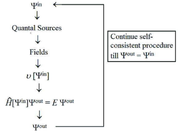
Figure 1: Procedure for the self-consistent solution of the Schrödinger equation.

In any self-consistent procedure, different external potentials $v({\bf{r}})$ can be obtained based on the choice of the initial approximate input wave function $\Psi({\bf{X}})$. In atoms, molecules or solids, the potential $v({\bf{r}})$ obtained self-consistently would be Coulombic. In quantum dots it would be harmonic, and so on. One must begin with an educated accurate guess apropos to the physical system of interest for the initial input. Otherwise one may not achieve self-consistency. Thus, for example, in self-consistent quantal density functional theory calculations on atoms 3 ; 13 ; 14 , the initial input wave function for an atom is the solution of the prior atom of the Periodic Table. In general, for any self-consistent calculation, it is only after self-consistency is achieved that one must judge and test whether the solution is physically meaningful. (Note that in this manner, the external potential $v({\bf{r}})$ and hence the Hamiltonian is determined self-consistently.)

In principle, the above procedure is mathematically entirely akin to the fully-self-consistent solution of the integro-differential equations of Hartree 9 and Hartree-Fock 10 theories, the Optimized Potential method 11 ; 12 , Quantal density functional theory 3 , etc. In each of these cases, the corresponding integro-differential equations are of the form $\hat{H}[\zeta_{i}]\zeta_{i}({\bf{x}})=\lambda_{i}\zeta_{i}({\bf{x}})$, where $\hat{H}$ is the corresponding Hamiltonian and $\zeta_{i},\lambda_{i}$ the single particle orbitals and eigenvalues, respectively. This eigenvalue equation is of the same form as that of the Schrödinger equation written in self-consistent form but with the generalization to the many-electron system. Thus, we now understand that the Schrödinger equation too can be thought of as being a self-consistent equation. This perspective of Schrödinger theory is new.

(We note that there exists a ‘Quantal Newtonian’ first law for Hartree, Hartree-Fock, and local effective potential theories 2 ; 3 . Hence, the external potential $v({\bf{r}})$ of these theories can also be expressed as the work done in a conservative field, and thus replaced in the corresponding equations by a known functional of the requisite Slater determinant.)

(vi) Observe that in writing the Schrödinger equation as in Eqs. (8), (9), the magnetic field ${\boldsymbol{\cal{B}}}({\bf{r}})$ now appears in the Hamiltonian explicitly via the Lorentz field ${\boldsymbol{\cal{L}}}({\bf{r}})$. (See Eq. (7).) It is the intrinsic self-consistent nature of the equation that demands the presence of ${\boldsymbol{\cal{B}}}({\bf{r}})$ in the Hamiltonian. In other words, as the Hamiltonian $\hat{H}[\Psi]$ is being determined self-consistently, all the information of the physical system – electrons and fields – must be incorporated in it. (Of course, equivalently the field ${\boldsymbol{\cal{B}}}({\bf{r}})$ could be expressed in terms of the vector potential ${\bf{A}}({\bf{r}})$. This then shows that when written in self-consistent form, there exists another component of the Hamiltonian involving the vector potential.)

(vii) The presence of a solely electrostatic external field ${\boldsymbol{\cal{E}}}({\bf{r}})=-{\boldsymbol{\nabla}}v({\bf{r}})$ is a special case of the stationary state theory discussed above. This case then constitutes the description of matter as defined previously.

IV Example of a Quantum Dot

To explicate the new physics of stationary-state Schrödinger theory, we consider a ground and first excited singlet state of a two electron, two-dimensional quantum dot in an external magnetostatic field 20 ; 21 . The external scalar potential in the Hamiltonian of Eq. (1) is then $v({\bf{r}})=\frac{1}{2}\omega^{2}_{0}r^{2}$, with $\omega_{0}$ the harmonic frequency. The ground $\psi_{0}({\bf{r}}_{1}{\bf{r}}_{2})$ 16 and excited $\psi_{1}({\bf{r}}_{1}{\bf{r}}_{2})$ 22 state wave functions of the quantum dot in the symmetric gauge ${\bf{A}}({\bf{r}})=\frac{1}{2}{\boldsymbol{\cal{B}}}({\bf{r}})\times{\bf{r}}$, are respectively,

$$\psi_{0}({\bf{r}}_{1}{\bf{r}}_{2})=C_{0}e^{-\Omega(R^{2}+\frac{1}{4}r^{2})}(1+r),$$ (10)

and

$$\psi_{1}({\bf{r}}_{1}{\bf{r}}_{2})=C_{1}e^{-\Omega(R^{2}+\frac{1}{4}r^{2})}\bigg{[}1 + r+\bigg{(}\frac{\Omega}{4}-0.436815\bigg{)}r^{2}$$ (11)

$$+ \bigg{(}\frac{\Omega}{4}-0.353786\bigg{)}r^{3}\bigg{]},$$

where ${\bf{R}}=({\bf{r}}_{1}+{\bf{r}}_{2})/2$, $r=|{\bf{r}}_{1}-{\bf{r}}_{2}|$, $C_{0}=\Omega^{\frac{3}{2}}/\pi[2+\Omega+\sqrt{2\pi\Omega}]^{\frac{1}{2}}$, $C_{1}=0.108563$, $\Omega=\sqrt{k_{\mathrm{eff}}}$, the effective force constant $k_{\mathrm{eff}}=\omega_{0}^{2}+\omega_{L}^{2}=1$ for the ground state, and $k_{\mathrm{eff}}=0.471716$ for the excited case, with $\omega_{L}=B/2$ the Larmor frequency, $E_{0}=3.000000$ a.u., $E_{1}=3.434076$ a.u..

In Figs. 2 and 3 we plot the corresponding electron-interaction ${\boldsymbol{\cal{E}}}_{\mathrm{ee}}({\bf{r}})$, kinetic ${\boldsymbol{\cal{Z}}}({\bf{r}})$, and differential density ${\boldsymbol{\cal{D}}}({\bf{r}})$ components of the internal ${\boldsymbol{\cal{F}}}^{\mathrm{int}}({\bf{r}})$ field. The total magnetic field contribution is incorporated into the effective force constant $k_{\mathrm{eff}}$. Observe that $-{\boldsymbol{\cal{E}}}_{\mathrm{ee}}({\bf{r}})+{\boldsymbol{\cal{Z}}}({\bf{r}})+{\boldsymbol{\cal{D}}}({\bf{r}})=-k_{\mathrm{eff}}r$. This then demonstrates the satisfaction of the ‘Quantal Newtonian’ first law of Eq. (4).

The example of the quantum dot above can be thought of as being the final iteration of the self-consistent procedure in which the exact potential $v({\bf{r}})$, wave function $\Psi$, and energy $E$ are obtained. To see this, consider the initial choice of wave functions to be the following:

$$\Psi_{0}({\bf{r}}_{1}{\bf{r}}_{2})=C_{0}e^{-\Omega_{0}(R^{2}+\frac{1}{4}r^{2})}(1+a_{0}r),$$ (12)

and

$$\Psi_{1}({\bf{r}}_{1}{\bf{r}}_{2})=C_{1}e^{-\Omega_{1}(R^{2}+\frac{1}{4}r^{2})}(1+a_{1}r+b_{1}r^{2}+c_{1}r^{3}),$$ (13)

where $C_{0},C_{1},\Omega_{0},\Omega_{1},a_{0},a_{1},b_{1},c_{1}$ are constants. Let us next assume that for some random iteration, the values of these coefficients turn out to be $C_{0}=0.135646$, $\Omega_{0}=1.000000$, $a_{0}=1.000000$; $C_{1}=0.108563$, $\Omega_{1}=0.686816$, $a_{1}=1.000000$, $b_{1}=-0.265111$, $c_{1}=-0.182082$. One then determines the various fields from the corresponding wave functions and plots them. On adding the fields ${\boldsymbol{\cal{D}}}({\bf{r}})$ and ${\boldsymbol{\cal{Z}}}({\bf{r}})$ one obtains the dot-dash lines as shown in Figs. 2 and 3 for (${\boldsymbol{\cal{D}}}({\bf{r}})+{\boldsymbol{\cal{Z}}}({\bf{r}})$). Adding $-{\boldsymbol{\cal{E}}}_{\mathrm{ee}}({\bf{r}})$ to these lines, one then obtains a straight (dashed) line $-k_{\mathrm{eff}}r$ in each case. On substituting this $-k_{\mathrm{eff}}r$ back into the Schrödinger equation and solving, one obtains the same wave functions $\Psi_{0},\Psi_{1}$ and energies $E_{0},E_{1}$ as that of Eqs. (10) and (11). Additionally, it becomes clear that the potential $v({\bf{r}})$ is harmonic. This then constitutes the final iteration of the self-consistency procedure.

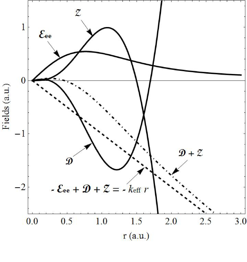
Figure 2: The electron-interaction ${\boldsymbol{\cal{E}}}_{\mathrm{ee}}({\bf{r}})$, kinetic ${\boldsymbol{\cal{Z}}}({\bf{r}})$, and differential density ${\boldsymbol{\cal{D}}}({\bf{r}})$ components of the internal field ${\boldsymbol{\cal{F}}}^{\mathrm{int}}({\bf{r}})$ for the ground state of a quantum dot in a magnetic field. The sums ${\boldsymbol{\cal{D}}}({\bf{r}})+{\boldsymbol{\cal{Z}}}({\bf{r}})$, and $-{\boldsymbol{\cal{E}}}_{\mathrm{ee}}({\bf{r}})+{\boldsymbol{\cal{Z}}}({\bf{r}})+{\boldsymbol{\cal{D}}}({\bf{r}})=-k_{\mathrm{eff}}r$ with $k_{\mathrm{eff}}=1$ are also plotted.

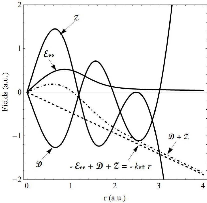
Figure 3: Same as in Fig. 2 but for the first excited singlet state with $k_{\mathrm{eff}}=0.471716$.

V Time-dependent Theory: ‘Quantal Newtonian’ Second Law

The above conclusions are generalizable to the TD case by considering the external field to be ${\boldsymbol{\cal{F}}}^{\mathrm{ext}}({\bf{r}}t)={\boldsymbol{\cal{E}}}({\bf{r}}t)=-{\boldsymbol{\nabla}}v({\bf{r}}t)$. In this case, the ‘Quantal Newtonian’ second law for each electron – the quantal equivalent to Newton’s second law of Eq. (2) – is 2 ; 4 ; 5

$${\boldsymbol{\cal{F}}}^{\mathrm{ext}}({\bf{r}}t)+{\boldsymbol{\cal{F}}}^{\mathrm{int}}({\bf{r}}t)={\boldsymbol{\cal{J}}}({\bf{r}}t),$$ (14)

where ${\boldsymbol{\cal{F}}}^{\mathrm{int}}({\bf{r}}t)$ is given by the TD version of Eq. (6) (without the ${\boldsymbol{\cal{I}}}({\bf{r}}t)$ term) and the response of the electron is described by the current density field ${\boldsymbol{\cal{J}}}({\bf{r}}t)=(1/\rho({\bf{r}}t))\partial{\bf{j}}({\bf{r}}t)/\partial t$. The corresponding external potential energy $v[\Psi]({\bf{r}}t)$ functional of the wave function $\Psi({\bf{X}}t)$ is then the work done at each instant of time in a conservative field:

$$v[\Psi]({\bf{r}}t)=\int^{\bf{r}}_{\infty}{\boldsymbol{\cal{F}}}({\bf{r}}^{\prime}t)\cdot d{\boldsymbol{\ell}}^{\prime},$$ (15)

where ${\boldsymbol{\cal{F}}}({\bf{r}}t)={\boldsymbol{\cal{F}}}^{\mathrm{int}}({\bf{r}}t)-{\boldsymbol{\cal{J}}}({\bf{r}}t)$, with the TD self-consistent Schrödinger equation being

$$\bigg{[}\frac{1}{2}\sum_{i}\hat{\bf{p}}_{i}^{2}+\frac{1}{2}\sideset{}{{}^{\prime}}{\sum}_{i,j}\frac{1}{|{\bf{r}}_{i}-{\bf{r}}_{j}|}+\sum_{i}v[\Psi]({\bf{r}}_{i}t)\bigg{]}\Psi({\bf{X}}t)=i\frac{\partial\Psi({\bf{X}}t)}{\partial t}.$$ (16)

Since ${\boldsymbol{\nabla}}\times{\boldsymbol{\cal{F}}}({\bf{r}}t)=0$, the work done $v({\bf{r}}t)$ at each instant of time is path-independent and thus a potential energy. Again, on summing Eq, (14) over all the electrons, the contribution of ${\boldsymbol{\cal{F}}}^{\mathrm{int}}({\bf{r}}t)$ vanishes, leading to Ehrenfest’s (second law) theorem $\int\rho({\bf{r}}t)[{\boldsymbol{\cal{F}}}^{\mathrm{ext}}({\bf{r}}t)-{\boldsymbol{\cal{J}}}({\bf{r}}t)]d{\bf{r}}=0$. The further generalization of the ‘Quantal Newtonian’ second law to the case of an external TD electromagnetic field with ${\boldsymbol{\cal{E}}}({\bf{r}})=-{\boldsymbol{\nabla}}v({\bf{r}})$, ${\bf{E}}({\bf{r}}t)=-{\boldsymbol{\nabla}}\phi({\bf{r}}t)-\partial{\bf{A}}({\bf{r}}t)/\partial t$, ${\boldsymbol{\cal{B}}}({\bf{r}}t)={\boldsymbol{\nabla}}\times{\bf{A}}({\bf{r}}t)$, is given in 7 .

As an example of the insights for the time-dependent case, consider the two-dimensional two-electron quantum dot in an external magnetostatic field ${\boldsymbol{\cal{B}}}({\bf{r}})={\boldsymbol{\nabla}}\times{\bf{A}}({\bf{r}})$ perturbed by a time-dependent electric field ${\bf{E}}(t)$. The wave function of this system 23 ; 24 , known as the Generalized Kohn Theorem, is comprised of a phase factor times the unperturbed wave function in which the coordinates of each electron are translated by a time-dependent function that satisfies the classical equation of motion. Hence, if the unperturbed wave function is known, the time evolution of all properties is known. As the wave functions for a ground and excited state of the unperturbed quantum dot are given by Eqs. (10), (11), the corresponding solutions of the time-dependent Schrödinger equation, and therefore of all the various fields, is obtained. At the initial time, $t=0$, the results are those of Figs. 2 and 3. Observables that are expectations of non-differential operators such as the density $\rho({\bf{r}}t)$, the electron-interaction field ${\boldsymbol{\cal{E}}}_{\mathrm{ee}}({\bf{r}}t)$, etc., are simply the time-independent functions shifted in time.

VI Concluding Remarks

In conclusion, we have arrived at new insights into the Schrödinger theory of electrons in electromagnetic fields via the ‘Quantal Newtonian’ first and second laws for each electron. A principal understanding is that the scalar potential energy of an electron $\{v({\bf{r}})/v({\bf{r}}t)\}$ is a known functional of the wave function $\{\Psi({\bf{X}})/\Psi({\bf{X}}t)\}$. As such the Hamiltonian $\{\hat{H}/\hat{H}(t)\}$ is a functional of the wave function: $\{\hat{H}[\Psi({\bf{X}})]/\hat{H}[\Psi({\bf{X}})t]\}$. Thus the Schrödinger equation can now be thought of as one whose solution can be obtained self-consistently. A path for the determination of the exact wave function is thus formulated. Such a path is feasible given the advent of present-day high computing power. A second understanding achieved is that it is now possible to write the scalar potential $[v({\bf{r}})/v({\bf{r}}t)]$ as the sum of component functions each of which is representative of a specific property of the system such as the correlations due to the Pauli exclusion principle and Coulomb repulsion, kinetic and magnetic effects, and the electron density. Such a property-related division of the scalar potential is shown by the example of the quantum dot in a magnetostatic field given in the text. Another interesting observation is that in its self-consistent form, in addition to the vector potential, which appears in the Schrödinger equation as a consequence of the correspondence principle, the magnetic field now too appears in the equation because of the ‘Quantal Newtonian’ laws. Ex post facto, we now understand that this must be the case as the Hamiltonian itself is being determined self-consistently.

It is interesting to compare the self-consistent method for the determination of the wave function in the stationary ground state case to that of the variational method. The latter is associated principally with the property of the total energy. An approximate parametrized variational wave function correct to $O(\delta)$ leads to an upper bound for the energy that is correct to $O(\delta^{2})$. Such a wave function is accurate in the region where the principal contribution to the energy arises. However, all other observables obtained as the expectation of Hermitian single- and two-particle operators are correct only to the same order as that of the wave function, viz. to $O(\delta)$. A better approximate variational wave function is one that leads to a lower value of the energy. There is no guarantee that other observables representative of different regions of configuration space are thereby more accurate. On the other hand, in the self-consistent procedure, achieved say to a desired accuracy of five decimal places, all the properties are correct to the same degree of accuracy. An improved wave function would be one correct to a greater decimal accuracy. As a point of note, the constrained-search variational method 25 ; 26 ; 27 expands the variational space of approximate parametrized wave functions by considering the wave function $\Psi$ to be a functional of a function $\chi$, i.e. $\Psi=\Psi[\chi]$. One searches over all functions $\chi$ such that the wave function $\Psi[\chi]$ is normalized, gives the exact (theoretical or experimental) value of an observable, while leading to a rigorous upper bound to the energy. In this manner, the wave function functional $\Psi[\chi]$ is accurate not only in the region contributing to the energy, but also that of the observable. The self-consistent solution of the Schrödinger equation, however, is accurate to the degree required, throughout configuration space.

We do not address here the broader procedural aspects of the self-consistency, nor the implications of the explicit presence of the magnetic field in it. These issues constitute current and future research.

The authors acknowledge Lou Massa and Marlina Slamet for their critique of the paper. VS is supported in part by the Research Foundation of the City University of New York. XP is supported by the National Natural Science Foundation of China (Grant No: 11275100).

References

- (1) V. Sahni and X.-Y. Pan, Bull. Am. Phys. Soc. 61, 408 (2016)
- (2) V. Sahni, Quantal Density Functional Theory, Springer-Verlag, Berlin, Heidelberg, (2004); 2nd edition (2016); and references to the original literature therein
- (3) V. Sahni, Quantal Density Functional Theory II: Approximation Methods and Applications, Springer-Verlag, Berlin, Heidelberg, (2010)
- (4) Z. Qian and V. Sahni, Phys. Let. A 247, 303 (1998)
- (5) Z. Qian and V. Sahni, Int. J. Quantum Chem. 78, 341 (2000)
- (6) Z. Qian and V. Sahni, Phys. Rev. A 63, 042508 (2001)
- (7) V. Sahni, X.-Y. Pan and T. Yang, Computation 4, 30 (2016); doi:10.3990/computation 4030030
- (8) A. Holas and N. H. March, Phys. Rev. A 51, 2040 (1995)
- (9) D.R. Hartree, The Calculation of Atomic Structures, Wiley, New York, (1957)
- (10) C.F. Fischer, The Hartree-Fock Theory for Atoms, Wiley, New York (1977)
- (11) J.D. Talman and W.F. Shadwick, Phys. Rev. A 14, 36 (1976)
- (12) E. Engel and S.H. Vosko, Phys. Rev. A 47, 2800 (1993)
- (13) V. Sahni, Z. Qian, and K.D. Sen, J. Chem. Phys. 114, 8784 (2001)
- (14) V. Sahni, Y. Li, and M.K. Harbola, Phys. Rev. A 45, 1434 (1992)
- (15) Y. Aharonov and D. Bohm, Phys. Rev. 54, 485 (1959)
- (16) T. Yang, X.-Y. Pan and V. Sahni, Phys. Rev. A 83, 042518 (2011)
- (17) A. Holas and N. H. March, Phys. Rev. A 56, 4595 (1997)
- (18) P. Hohenberg and W. Kohn, Phys. Rev. 136, B864 (1964)
- (19) W. Kohn and L. J. Sham, Phys. Rev. 140, A1133 (1965)
- (20) M. Taut, J. Phys. A 27, 1045 (1994); 27, 4723 (1994)
- (21) M. Taut and H. Eschrig, Z. Phys. Chem. 224, 631 (2010)
- (22) M. Slamet and V. Sahni Bull. Am. Phys. Soc. 61, 367 (2016); (manuscript in preparation)
- (23) H.-M. Zhu, J.-W. Chen, X.-Y. Pan, and V. Sahni, J. Chem Phys. 140, 024318 (2014)
- (24) W. Kohn, Phys. Rev. 123, 1242 (1961)
- (25) X.-Y. Pan, V. Sahni, and L. Massa, Phys. Rev Lett. 93, 130401 (2004)
- (26) X.-Y. Pan, M. Slamet, and V. Sahni, Phys. Rev. A 81, 042524 (2010)
- (27) M. Slamet, X.-Y. Pan, and V. Sahni, Phys. Rev A 84, 052504 (2011)