GRAM: Graph-based Attention Model for Healthcare Representation Learning

Abstract

Deep learning methods exhibit promising performance for predictive modeling in healthcare, but two important challenges remain:

• Data insufficiency: Often in healthcare predictive modeling, the sample size is insufficient for deep learning methods to achieve satisfactory results.

• Interpretation: The representations learned by deep learning methods should align with medical knowledge.

To address these challenges, we propose a GRaph-based Attention Model, GRAM that supplements electronic health records (EHR) with hierarchical information inherent to medical ontologies. Based on the data volume and the ontology structure, GRAM represents a medical concept as a combination of its ancestors in the ontology via an attention mechanism.

We compared predictive performance (i.e. accuracy, data needs, interpretability) of GRAM to various methods including the recurrent neural network (RNN) in two sequential diagnoses prediction tasks and one heart failure prediction task. Compared to the basic RNN, GRAM achieved 10% higher accuracy for predicting diseases rarely observed in the training data and 3% improved area under the ROC curve for predicting heart failure using an order of magnitude less training data. Additionally, unlike other methods, the medical concept representations learned by GRAM are well aligned with the medical ontology. Finally, GRAM exhibits intuitive attention behaviors by adaptively generalizing to higher level concepts when facing data insufficiency at the lower level concepts.

1 Introduction

The rapid growth in volume and diversity of health care data from electronic health records (EHR) and other sources is motivating the use of predictive modeling to improve care for individual patients. In particular, novel applications are emerging that use deep learning methods such as word embedding (Choi et al., 2016c; Choi et al., 2016d), recurrent neural networks (RNN) (Che et al., 2016; Choi et al., 2016a, b; Lipton et al., 2016), convolutional neural networks (CNN) (Nguyen et al., 2016) or stacked denoising autoencoders (SDA) (Che et al., 2015; Miotto et al., 2016), demonstrating significant performance enhancement for diverse prediction tasks. Deep learning models appear to perform significantly better than logistic regression or multilayer perceptron (MLP) models that depend, to some degree, on expert feature construction (Lipton et al., 2015; Razavian et al., 2016).

Training deep learning models typically requires large amounts of data that often cannot be met by a single health system or provider organization. Sub-optimal model performance can be particularly challenging when the focus of interest is predicting onset of a rare disease. For example, using Doctor AI (Choi et al., 2016a), we discovered that RNN alone was ineffective to predict the onset of diseases such as cerebral degenerations (e.g. Leukodystrophy, Cerebral lipidoses) or developmental disorders (e.g. autistic disorder, Heller’s syndrome), partly because their rare occurrence in the training data provided little learning opportunity to the flexible models like RNN.

The data requirement of deep learning models comes from having to assess exponential number of combinations of input features. This can be alleviated by exploiting medical ontologies that encodes hierarchical clinical constructs and relationships among medical concepts. Fortunately, there are many well-organized ontologies in healthcare such as the International Classification of Diseases (ICD), Clinical Classifications Software (CCS) (Stearns et al., 2001) or Systematized Nomenclature of Medicine-Clinical Terms (SNOMED-CT) (Project et al., 2010). Nodes (i.e. medical concepts) close to one another in medical ontologies are likely to be associated with similar patients, allowing us to transfer knowledge among them. Therefore, proper use of medical ontologies will be helpful when we lack enough data for the nodes in the ontology to train deep learning models.

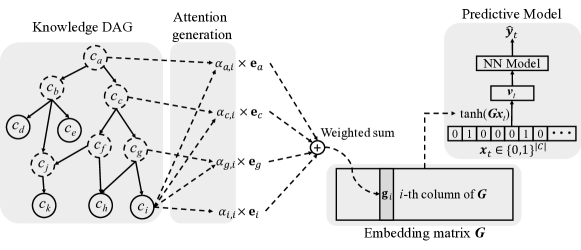
Figure 1: The illustration of GRAM. Leaf nodes (solid circles) represents a medical concept in the EHR, while the non-leaf nodes (dotted circles) represent more general concepts. The final representation $\mathbf{g}_{i}$ of the leaf concept $c_{i}$ is computed by combining the basic embeddings $\mathbf{e}_{i}$ of $c_{i}$ and $\mathbf{e}_{g},\mathbf{e}_{c}$ and $\mathbf{e}_{a}$ of its ancestors $c_{g},c_{c}$ and $c_{a}$ via an attention mechanism. The final representations form the embedding matrix $\mathbf{G}$ for all leaf concepts. After that, we use $\mathbf{G}$ to embed patient visit vector $\mathbf{x}_{t}$ to a visit representation $\mathbf{v}_{t}$, which is then fed to a neural network model to make the final prediction $\hat{\mathbf{y}}_{t}$.

In this work, we propose GRAM, a method that infuses information from medical ontologies into deep learning models via neural attention. Considering the frequency of a medical concept in the EHR data and its ancestors in the ontology, GRAM decides the representation of the medical concept by adaptively combining its ancestors via attention mechanism. This will not only support deep learning models to learn robust representations without large amount of data, but also learn interpretable representations that align well with the knowledge from the ontology. The attention mechanism is trained in an end-to-end fashion with the neural network model that predicts the onset of disease(s). We also propose an effective initialization technique in addition to the ontological knowledge to better guide the representation learning process.

We compare predictive performance (i.e. accuracy, data needs, interpretability) of GRAM to various models including the recurrent neural network (RNN) in two sequential diagnoses prediction tasks and one heart failure (HF) prediction task. We demonstrate that GRAM is up to 10% more accurate than the basic RNN for predicting diseases less observed in the training data. After discussing GRAM’s scalability, we visualize the representations learned from various models, where GRAM provides more intuitive representations by grouping similar medical concepts close to one another. Finally, we show GRAM’s attention mechanism can be interpreted to understand how it assigns the right amount of attention to the ancestors of each medical concept by considering the data availability and the ontology structure.

2 Methodology

We first define the notations describing EHR data and medical ontologies, followed by a description of GRAM (Section 2.2), the end-to-end training of the attention generation and predictive modeling (Section 2.3), and the efficient initialization scheme (Section 2.4).

2.1 Basic Notation

We denote the set of entire medical codes from the EHR as $c_{1},c_{2},\ldots,$ $c_{|\mathcal{C}|}\in\mathcal{C}$ with the vocabulary size $|\mathcal{C}|$. The clinical record of each patient can be viewed as a sequence of visits $V_{1},\ldots,V_{T}$ where each visit contains a subset of medical codes $V_{t}\subseteq\mathcal{C}$. $V_{t}$ can be represented as a binary vector $\mathbf{x}_{t}\in\{0,1\}^{|\mathcal{C}|}$ where the $i$-th element is 1 only if $V_{t}$ contains the code $c_{i}$. To avoid clutter, all algorithms will be presented for a single patient.

We assume that a given medical ontology $\mathcal{G}$ typically expresses the hierarchy of various medical concepts in the form of a parent-child relationship, where the medical codes $\mathcal{C}$ form the leaf nodes. Ontology $\mathcal{G}$ is represented as a directed acyclic graph (DAG) whose nodes form a set $\mathcal{D}=\mathcal{C}+\mathcal{C^{\prime}}$. The set $\mathcal{C^{\prime}}=\{c_{|\mathcal{C}|+1},c_{|\mathcal{C}|+2},\ldots,c_{|\mathcal{C}|+|\mathcal{C^{\prime}}|}\}$ consists of all non-leaf nodes (i.e. ancestors of the leaf nodes), where $|\mathcal{C^{\prime}}|$ represents the number of all non-leaf nodes. We use knowledge DAG to refer to $\mathcal{G}$. A parent in the knowledge DAG $\mathcal{G}$ represents a related but more general concept over its children. Therefore, $\mathcal{G}$ provides a multi-resolution view of medical concepts with different degrees of specificity. While some ontologies are exclusively expressed as parent-child hierarchies (e.g. ICD-9, CCS), others are not. For example, in some instances SNOMED-CT also links medical concepts to causal or treatment relationships, but the majority relationships in SNOMED-CT are still parent-child. Therefore, we focus on the parent-child relationships in this work.

2.2 Knowledge DAG and the Attention Mechanism

GRAM leverages the parent-child relationship of $\mathcal{G}$ to learn robust representations when data volume is constrained. GRAM balances the use of ontology information in relation to data volume in determining the level of specificity for a medical concept. When a medical concept is less observed in the data, more weight is given to its ancestors as they can be learned more accurately and offer general (coarse-grained) information about their children. The process of resorting to the parent concepts can be automated via the attention mechanism and the end-to-end training as described in Figure 1.

In the knowledge DAG, each node $c_{i}$ is assigned a basic embedding vector $\mathbf{e}_{i}\in\mathbb{R}^{m}$, where $m$ represents the dimensionality. Then $\mathbf{e}_{1},\ldots,\mathbf{e}_{|\mathcal{C}|}$ are the basic embeddings of the codes $c_{1},\ldots,c_{|\mathcal{C}|}$ while $\mathbf{e}_{|\mathcal{C}|+1},\ldots,\mathbf{e}_{|\mathcal{C}|+|\mathcal{C^{\prime}}|}$ represent the basic embeddings of the internal nodes $c_{|\mathcal{C}|+1},\ldots,c_{|\mathcal{C}|+|\mathcal{C^{\prime}}|}$. The initialization of these basic embeddings is described in Section 2.4. We formulate a leaf node’s final representation as a convex combination of the basic embeddings of itself and its ancestors:

$$\mathbf{g}_{i}=\sum_{j\in\mathcal{A}(i)}\alpha_{ij}\mathbf{e}_{j},\qquad\sum_{j\in\mathcal{A}(i)}\alpha_{ij}=1,~{}~{}\alpha_{ij}\geq 0~{}\text{ for }j\in\mathcal{A}(i),$$ (1)

where $\mathbf{g}_{i}\in\mathbb{R}^{m}$ denotes the final representation of the code $c_{i}$, $\mathcal{A}(i)$ the indices of the code $c_{i}$ and $c_{i}$’s ancestors, $\mathbf{e}_{j}$ the basic embedding of the code $c_{j}$ and $\alpha_{ij}\in\mathbb{R}$ the attention weight on the embedding $\mathbf{e}_{j}$ when calculating $\mathbf{g}_{i}$. The attention weight $\alpha_{ij}$ in Eq. (1) is calculated by the following Softmax function,

$$\alpha_{ij}=\frac{\exp(f(\mathbf{e}_{i},\mathbf{e}_{j}))}{\sum_{k\in\mathcal{A}(i)}\exp(f(\mathbf{e}_{i},\mathbf{e}_{k}))}$$ (2)

$f(\mathbf{e}_{i},\mathbf{e}_{j})$ is a scalar value representing the compatibility between the basic embeddings of $\mathbf{e}_{i}$ and $\mathbf{e}_{k}$. We compute $f(\mathbf{e}_{i},\mathbf{e}_{j})$ via the following feed-forward network with a single hidden layer (MLP),

$$f(\mathbf{e}_{i},\mathbf{e}_{j})=\mathbf{u}_{a}^{\top}\tanh(\mathbf{W}_{a}\left[\begin{array}[]{c}\mathbf{e}_{i}\\ \mathbf{e}_{j}\end{array}\right]+\mathbf{b}_{a})$$ (3)

where $\mathbf{W}_{a}\in\mathbb{R}^{l\times 2m}$ is the weight matrix for the concatenation of $\mathbf{e}_{i}$ and $\mathbf{e}_{j}$, $\mathbf{b}\in\mathbb{R}^{l}$ the bias vector, and $\mathbf{u}_{a}\in\mathbb{R}^{l}$ the weight vector for generating the scalar value. The constant $l$ represents the dimension size of the hidden layer of $f(\cdot,\cdot)$. We always concatenate $\mathbf{e}_{i}$ and $\mathbf{e}_{j}$ in the child-ancestor order. Note that the compatibility function $f$ is an MLP, because MLP is well known to be a sufficient approximator for an arbitrary function, and we empirically found that our formulation performed better in our use cases than alternatives such as inner product and Bahdanau et al.’s (Bahdanau et al., 2014).

Remarks: The example in Figure 1 is derived based on a single path from $c_{i}$ to $c_{a}$. However, the same mechanism can be applicable to multiple paths as well. For example, code $c_{k}$ has two paths to the root $c_{a}$, containing five ancestors in total. Another scenario is where the EHR data contain both leaf codes and some ancestor codes. We can move those ancestors present in EHR data from the set $\mathcal{C^{\prime}}$ to $\mathcal{C}$ and apply the same process as Eq. (1) to obtain the final representations for them.

2.3 End-to-End Training with a Predictive Model

We train the attention mechanism together with a predictive model such that the attention mechanism improves the predictive performance. By concatenating final representation $\mathbf{g}_{1},\mathbf{g}_{2},\ldots,\mathbf{g}_{|\mathcal{C}|}$ of all medical codes, we have the embedding matrix $\mathbf{G}\in\mathcal{R}^{m\times|\mathcal{C}|}$ where $\mathbf{g}_{i}$ is its $i$-th column of $\mathbf{G}$. We can then convert visit $V_{t}$ to a visit representation $\mathbf{v}_{t}$ by multiplying embedding matrix $\mathbf{G}$ with multi-hot vector $\mathbf{x}_{t}$ indicating the clinical events in visit $V_{t}$ as shown in the right side of Figure 1. Finally the visit representation $\mathbf{v}_{t}$ will be used as an input to pass to a predictive model for predicting the target label $\mathbf{y}_{t}$ using a neural network (NN) model. In this work, we use RNN as the choice of the NN model as the task is to perform sequential diagnoses prediction (Choi et al., 2016a, b) with the objective of predicting the disease codes of the next visit $V_{t+1}$ given the visit records up to the current timestep $V_{1},V_{2},\ldots,V_{t}$, which can be expressed as follows,

$$\widehat{\mathbf{y}}_{t}=\widehat{\mathbf{x}}_{t+1} =\mathrm{Softmax}(\mathbf{W}\mathbf{h}_{t}+\mathbf{b}),\text{\quad where}$$

$$\mathbf{h}_{1},\mathbf{h}_{2},\ldots,\mathbf{h}_{t} =\textrm{RNN}(\mathbf{v}_{1},\mathbf{v}_{2},\ldots,\mathbf{v}_{t};\theta_{r}),\text{\quad where}$$ (4)

$$\mathbf{v}_{1},\mathbf{v}_{2},\ldots,\mathbf{v}_{t} =\tanh(\mathbf{G}[\mathbf{x}_{1},\mathbf{x}_{2},\ldots,\mathbf{x}_{t}])$$

where $\mathbf{x}_{t}\in\mathbb{R}^{|\mathcal{C}|}$ denotes the $t$-th visit; $\mathbf{v}_{t}\in\mathbb{R}^{m}$ the $t$-th visit representation; $\mathbf{h}_{t}\in\mathbb{R}^{r}$ the RNN’s hidden layer at $t$-th time step (i.e. $t$-th visit); $\theta_{r}$ RNN’s parameters; $\mathbf{W}\in\mathbb{R}^{|\mathcal{C}|\times r}$ and $\mathbf{b}\in\mathbb{R}^{|\mathcal{C}|}$ the weight matrices and the bias vector of the Softmax function; $r$ denotes the dimension size of the hidden layer. We use “$\mathrm{RNN}$” to denote any recurrent neural network variants that can cope with the vanishing gradient problem (Bengio et al., 1994), such as LSTM (Hochreiter and Schmidhuber, 1997), GRU (Cho et al., 2014), and IRNN (Le et al., 2015), with any varying numbers of hidden layers. The prediction loss for all time steps is calculated using the binary cross entropy as follows,

$$\mathcal{L}(\mathbf{x}_{1},\mathbf{x}_{2}\ldots,\mathbf{x}_{T})=-\frac{1}{T-1}\sum_{t=1}^{T-1}\Big{(}{\mathbf{y}_{t}}^{\top}\log(\widehat{\mathbf{y}}_{t})+(\mathbf{1}-\mathbf{y}_{t})^{\top}\log(\mathbf{1}-\widehat{\mathbf{y}}_{t})\Big{)}$$ (5)

where we sum the cross entropy errors from all timestamps of $\widehat{\mathbf{y}}_{t}$, $T$ denotes the number of timestamps of the visit sequence. Note that the above loss is defined for a single patient. In actual implementation, we will take the average of the individual loss for multiple patients. Algorithm 1 describes the overall training procedure of GRAM, under the assumption that we are performing the sequential diagnoses prediction task using an RNN. Note that Algorithm 1 describes stochastic gradient update to avoid clutter, but it can be easily extended to other gradient based optimization such as mini-batch gradient update.

Algorithm 1 GRAM Optimization

  Randomly initialize basic embedding matrix $\mathbf{E}$, attention parameters $\mathbf{u}_{a},\mathbf{W}_{a},\mathbf{b}_{a}$, RNN parameter $\theta_{r}$, softmax parameters $\mathbf{W},\mathbf{b}$.

  repeat

     Update $\mathbf{E}$ with GloVe objective function (see Section 2.4)

  until convergence

  repeat

     $\mathbf{X}\leftarrow$ random patient from dataset

     for visit $V_{t}$ in $\mathbf{X}$ do

        for code $c_{i}$ in $V_{t}$ do

           Refer $\mathcal{G}$ to find $c_{i}$’s ancestors $C^{\prime}$

           for code $c_{j}$ in $C^{\prime}$ do

              Calculate attention weight $\alpha_{ij}$ using Eq. (2).

           end for

           Obtain final representation $\mathbf{g}_{i}$ using Eq. (1).

        end for

        $\mathbf{v}_{t}\leftarrow\mbox{tanh}(\sum_{i:c_{i}\in V_{t}}\mathbf{g}_{i})$

        Make prediction $\widehat{\mathbf{y}}_{t}$ using Eq. (4)

     end for

     Calculate prediction loss $\mathcal{L}$ using Eq .(5)

     Update parameters according to the gradient of $\mathcal{L}$

  until convergence

2.4 Initializing Basic Embeddings

The attention generation mechanism in Section 2.2 requires basic embeddings $\mathbf{e}_{i}$ of each node in the knowledge DAG. The basic embeddings of ancestors, however, pose a difficulty because they are often not observed in the data. To properly initialize them, we use co-occurrence information to learn the basic embeddings of medical codes and their ancestors. Co-occurrence has proven to be an important source of information when learning representations of words or medical concepts (Mikolov et al., 2013; Choi et al., 2016c; Choi et al., 2016d). To train the basic embeddings, we employ GloVe (Pennington et al., 2014), which uses the global co-occurrence matrix of words to learn their representations. In our case, the co-occurrence matrix of the codes and the ancestors was generated by counting the co-occurrences within each visit $V_{t}$, where we augment each visit with the ancestors of the codes in the visit.

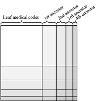
Figure 2: Creating the co-occurrence matrix together with the ancestors. The $n$-th ancestors are the group of nodes that are $n$ hops away from any leaf node in $\mathcal{G}$. Here we exclude the root node, which will be just a single row (column).

We describe the details of the initialization algorithm with an example. We borrow the parent-child relationships from the knowledge DAG of Figure 1. Given a visit $V_{t}$,

$$V_{t}=\{c_{d},c_{i},c_{k}\}$$

we augment it with the ancestors of all the codes to obtain the augmented visit $V^{\prime}_{t}$,

$$V^{\prime}_{t}=\{c_{d},\underline{c_{b}},\underline{c_{a}},c_{i},\underline{c_{g}},\underline{c_{c}},\underline{c_{a}},c_{k},\underline{c_{j}},\underline{c_{f}},\underline{c_{c}},\underline{c_{b}},\underline{c_{a}}\}$$

where the augmented ancestors are underlined. Note that a single ancestor can appear multiple times in $V^{\prime}_{t}$. In fact, the higher the ancestor is in the knowledge DAG, the more times it is likely to appear in $V^{\prime}_{t}$. We count the co-occurrence of two codes in $V^{\prime}_{t}$ as follows,

$$co\mbox{-}occurrence(c_{i},c_{j},V^{\prime}_{t})=count(c_{i},V^{\prime}_{t})\times count(c_{j},V^{\prime}_{t})$$

where $count(c_{i},V^{\prime}_{t})$ is the number of times the code $c_{i}$ appears in the augmented visit $V^{\prime}_{t}$. For example, the co-occurrence between the leaf code $c_{i}$ and the root $c_{a}$ is 3. However, the co-occurrence between the ancestor $c_{c}$ and the root $c_{a}$ is 6. Therefore our algorithm will make the higher ancestor codes, which are more general concepts, have more involvement in all medical events (i.e. visits), which is natural in healthcare application as those general concepts are often reliable. We repeat this calculation for all pairs of codes in all augmented visits of all patients to obtain the co-occurrence matrix $\mathbf{M}\in\mathbb{R}^{|\mathcal{D}|\times|\mathcal{D}|}$ depicted by Figure 2. For training the embedding vectors $\mathbf{e}_{i}$’s using $\mathbf{M}$, we minimize the following loss function as described in Pennington et al. (2014).

$$J =\sum_{i,j=1}^{|\mathcal{D}|}f(\mathbf{M}_{ij})(\mathbf{e}_{i}^{\top}\mathbf{e}_{j}+b_{i}+b_{j}-\log\mathbf{M}_{ij})^{2}$$

where $$f(x)=\begin{cases}(x<x_{max})^{\alpha}&\text{if $x<x_{max}$}\\ 1&\text{otherwise}\end{cases}$$

where the hyperparameters $x_{max}$ and $\alpha$ are respectively set to $100$ and $0.75$ as the original paper (Pennington et al., 2014). Note that, after the initialization, the basic embeddings $\mathbf{e}_{i}$’s of both leaf nodes (i.e. medical codes) and non-leaf nodes (i.e. ancestors) are fine-tuned during model training via backpropagation.

3 Experiments

We conduct three experiments to determine if GRAM offered superior prediction performance when facing data insufficiency. We first describe the experimental setup followed by results comparing predictive performance of GRAM with various baseline models. After discussing GRAM’s scalability, we qualitatively evaluate the interpretability of the resulting representation. The source code of GRAM is publicly available at https://github.com/mp2893/gram.

3.1 Experiment Setup

Table 1: Basic statistics of Sutter PAMF, MIMIC-III and Sutter heart failure (HF) cohort.

Dataset	Sutter PAMF	MIMIC-III	Sutter HF cohort
# of patients	258,555†	7,499†	30,727† (3,408 cases)
# of visits	13,920,759	19,911	572,551
Avg. # of visits per patient	53.8	2.66	38.38
# of unique ICD9 codes	10,437	4,893	5,689
Avg. # of codes per visit	1.98	13.1	2.06
Max # of codes per visit	54	39	29
$\dagger$ For all datasets, we chose patients who made at least two visits.

Prediction tasks and source of data: We conduct the sequential diagnoses prediction (SDP) tasks on two datasets, which aim at predicting all diagnosis categories in the next visit, and a heart failure (HF) prediction task on one dataset, which is a binary prediction task for predicting a future HF onset where the prediction is made only once at the last visit $\mathbf{x}_{T}$.
Two sequential diagnoses predictions (SDP) are respectively conducted using two datasets: 1) Sutter Palo Alto Medical Foundation (PAMF) dataset, which consists of 18-years longitudinal medical records of 258K patients between age 50 and 90. This will determine GRAM’s performance for general adult population with long visit records. 2) MIMIC-III dataset (Johnson et al., 2016; Goldberger et al., 2000), which is a publicly available dataset consisting of medical records of 7.5K intensive care unit (ICU) patients over 11 years. This will determine GRAM’s performance for high-risk patients with very short visit records. We utilize all the patients with at least 2 visits. We prepared the true labels $\mathbf{y}_{t}$ by grouping the ICD9 codes into 283 groups using CCS single-level diagnosis grouper. This is to improve the training speed and predictive performance for easier analysis, while preserving sufficient granularity for each diagnosis. Each diagnosis code’s varying frequency in the training data can be viewed as different degrees of data insufficiency. We calculate Accuracy@k for each of CCS single-level diagnosis codes such that, given a visit $V_{t}$, we get 1 if the target diagnosis is in the top $k$ guesses and 0 otherwise.
We conduct HF prediction on Sutter heart failure (HF) cohort, which is a subset of Sutter PAMF data for a heart failure onset prediction study with 3.4K HF cases chosen by a set of criteria described in Vijayakrishnan et al. (2014); Gurwitz et al. (2013) and 27K matching controls chosen by a set of criteria described in Choi et al. (2016e). This will determine GRAM’s performance for a different prediction task where we predict the onset of one specific condition. We randomly downsample the training data to create different degrees of data insufficiency. We use area under the ROC curve (AUC) to measure the performance.
A summary of the datasets are provided in Table 1.We used CCS multi-level diagnoses hierarchy as our knowledge DAG $\mathcal{G}$. We also tested the ICD9 code hierarchy, but the performance was similar to using CCS multi-level hierarchy. For all three tasks, we randomly divide the dataset into the training, validation and test set by .75:.10:.15 ratio, and use the validation set to tune the hyper-parameters. Further details regarding the hyper-parameter tuning are provided below. The test set performance is reported in the paper.

Implementation details: We implemented GRAM with Theano 0.8.2 (Team, 2016). For training models, we used Adadelta (Zeiler, 2012) with a mini-batch of 100 patients, on a machine equipped with Intel Xeon E5-2640, 256GB RAM, four Nvidia Titan X’s and CUDA 7.5.

Models for comparison are the following. The first two GRAM+ and GRAM are the proposed methods and the rest are baselines. Hyper-parameter tuning is configured so that the number of parameters for the baselines would be comparable to GRAM’s. Further details are provided below.

• GRAM: Input sequence $\mathbf{x}_{1},\ldots,\mathbf{x}_{T}$ is first transformed by the embedding matrix $\mathbf{G}$, then fed to the GRU with a single hidden layer, which in turn makes the prediction, as described by Eq. (4). The basic embeddings $\mathbf{e}_{i}$’s are randomly initialized.

• GRAM+: We use the same setup as GRAM, but the basic embeddings $\mathbf{e}_{i}$’s are initialized according to Section 2.4.

• RandomDAG: We use the same setup as GRAM, but each leaf concept has five randomly assigned ancestors from the CCS multi-level hierarchy to test the effect of correct domain knowledge.

• RNN: Input $\mathbf{x}_{t}$ is transformed by an embedding matrix $\mathbf{W}_{emb}\in\mathbb{R}^{k\times|\mathcal{C}|}$, then fed to the GRU with a single hidden layer. The embedding size $k$ is a hyper-parameter. $\mathbf{W}_{emb}$ is randomly initialized and trained together with the GRU.

• RNN+: We use the RNN model with the same setup as before, but we initialize the embedding matrix $\mathbf{W}_{emb}$ with GloVe vectors trained only with the co-occurrence of leaf concepts. This is to compare GRAM with a similar weight initialization technique.

• SimpleRollUp: We use the RNN model with the same setup as before. But for input $\mathbf{x}_{t}$, we replace all diagnosis codes with their direct parent codes in the CCS multi-level hierarchy, giving us 578, 526 and 517 input codes respectively for Sutter data, MIMIC-III and Sutter HF cohort. This is to compare the performance of GRAM with a common grouping technique.

• RollUpRare: We use the RNN model with the same setup as before, but we replace any diagnosis code whose frequency is less than a certain threshold in the dataset with its direct parent. We set the threshold to 100 for Sutter data and Sutter HF cohort, and 10 for MIMIC-III, giving us 4,408, 935 and 1,538 input codes respectively for Sutter data, MIMIC-III and Sutter HF cohort. This is an intuitive way of dealing with infrequent medical codes.

Hyper-parameter Tuning: We define five hyper-parameters for GRAM:

• dimensionality $m$ of the basic embedding $\mathbf{e}_{i}$: [100, 200, 300, 400, 500]

• dimensionality $r$ of the RNN hidden layer $\mathbf{h}_{t}$ from Eq. (4): [100, 200, 300, 400, 500]

• dimensionality $l$ of $\mathbf{W}_{a}$ and $\mathbf{b}_{a}$ from Eq. (3): [100, 200, 300, 400, 500]

• $L_{2}$ regularization coefficient for all weights except RNN weights: [0.1, 0.01, 0.001, 0.0001]

• dropout rate for the dropout on the RNN hidden layer: [0.0, 0.2, 0.4, 0.6, 0.8]

We performed 100 iterations of the random search by using the above ranges for each of the three prediction experiments. In order to fairly compare the model performances, we matched the number of model parameters to be similar for all baseline methods. To facilitate reproducibility, final hyper-parameter settings we used for all models for each prediction experiments are described at the source code repository, https://github.com/mp2893/gram, along with the detailed steps we used to tune the hyper-parameters.

3.2 Prediction performance and scalability

Model	0-20	20-40	40-60	60-80	80-100
GRAM+	0.0150	0.3242	0.4325	0.4238	0.4903
GRAM	0.0042	0.2987	0.4224	0.4193	0.4895
RandomDAG	0.0050	0.2700	0.4010	0.4059	0.4853
RNN+	0.0069	0.2742	0.4140	0.4212	0.4959
RNN	0.0080	0.2691	0.4134	0.4227	0.4951
SimpleRollUp	0.0085	0.3078	0.4369	0.4330	0.4924
RollUpRare	0.0062	0.2768	0.4176	0.4226	0.4956

(a) Accuracy@5 of sequential diagnoses prediction on Sutter data

Model	0-20	20-40	40-60	60-80	80-100
GRAM+	0.0672	0.1787	0.2644	0.2490	0.6267
GRAM	0.0556	0.1016	0.1935	0.2296	0.6363
RandomDAG	0.0329	0.0708	0.1346	0.1512	0.4494
RNN+	0.0454	0.0843	0.2080	0.2494	0.6239
RNN	0.0454	0.0731	0.1804	0.2371	0.6243
SimpleRollUp	0.0578	0.1328	0.2455	0.2667	0.6387
RollUpRare	0.0454	0.0653	0.1843	0.2364	0.6277

(b) Accuracy@20 of sequential diagnoses prediction on MIMIC-III

Model	10%	20%	30%	40%	50%	60%	70%	80%	90%	100%
GRAM+	0.7970	0.8223	0.8307	0.8332	0.8389	0.8404	0.8452	0.8456	0.8447	0.8448
GRAM	0.7981	0.8217	0.8340	0.8332	0.8372	0.8377	0.8440	0.8431	0.8430	0.8447
RandomDAG	0.7644	0.7882	0.7986	0.8070	0.8143	0.8185	0.8274	0.8312	0.8254	0.8226
RNN+	0.7930	0.8117	0.8162	0.8215	0.8261	0.8333	0.8343	0.8353	0.8345	0.8335
RNN	0.7811	0.7942	0.8066	0.8111	0.8156	0.8207	0.8258	0.8278	0.8297	0.8314
SimpleRollUp	0.7799	0.8022	0.8108	0.8133	0.8177	0.8207	0.8223	0.8272	0.8269	0.8258
RollUpRare	0.7830	0.8067	0.8064	0.8119	0.8211	0.8202	0.8262	0.8296	0.8307	0.8291

(c) AUC of HF onset prediction on Sutter HF cohort

Table 2: Performance of three prediction tasks. The x-axis of (a) and (b) represents the labels grouped by the percentile of their frequencies in the training data in non-decreasing order. 0-20 are the most rare diagnosese while 80-100 are the most common ones. (b) uses Accuracy@20 because MIMIC-III has a large average number of codes per visit (see Table 1). For (c), we vary the size of the training data to train the models.

Tables 2(a) and 2(b) show the sequential diagnoses prediction performance on Sutter data and MIMIC-III. Both figures show that GRAM+ outperforms other models when predicting labels with significant data insufficiency (i.e. less observed in the training data).The performance gain is greater for MIMIC-III, where GRAM+ outperforms the basic RNN by 10% in the 20th-40th percentile range. This seems to come from the fact that MIMIC patients on average have significantly shorter visit history than Sutter patients, with much more codes received per visit. Such short sequences make it difficult for the RNN to learn and predict diagnoses sequence. The performance difference between GRAM+ and GRAM suggests that our proposed initialization scheme of the basic embeddings $\mathbf{e}_{i}$ is important for sequential diagnosis prediction.

Table 2(c) shows the HF prediction performance on Sutter HF cohort. GRAM and GRAM+ consistently outperforms other baselines (except RNN+) by 3$\sim$4% AUC, and RNN+ by maximum 1.8% AUC. These differences are quite significant given that the AUC is already in the mid-80s, a high value for HF prediction, cf. (Choi et al., 2016e). Note that, for GRAM+ and RNN+, we used the downsampled training data to initialize the basic embeddings $\mathbf{e}_{i}$’s and the embedding matrix $\mathbf{W}_{emb}$ with GloVe, respectively. The result shows that the initialization scheme of the basic embeddings in GRAM+ gives limited improvement over GRAM. This stems from the different natures of the two prediction tasks. While the goal of HF prediction is to predict a binary label for the entire visit sequence, the goal of sequential diagnosis prediction is to predict the co-occurring diagnosis codes at every visit. Therefore the co-occurrence information infused by the initialized embedding scheme is more beneficial to sequential diagnosis prediction. Additionally, this benefit is associated with the natures of the two prediction tasks than the datasets used for the prediction tasks. Because the initialized embedding shows different degrees of improvement as shown by Tables 2(a) and 2(c), when Sutter HF cohort is a subset of Sutter PAMF, thus having similar characteristics.

Table 3: Scalablity result in per epoch training time in second (the number of epochs needed). SDP stands for Sequential Diagnoses Prediction

Model	SDP (Sutter data)	SDP (MIMIC-III)	HF prediction (Sutter HF cohort)
GRAM	525s (39 epochs)	2s (11 epochs)	12s (7 epochs)
RNN	352s (24 epochs)	1s (6 epochs)	8s (5 epochs)

Overall, GRAM showed superior predictive performance under data insufficiency in three different experiments, demonstrating its general applicability in clinical predictive modeling. Now we briefly discuss the scalability of GRAM by comparing its training time to RNN’s. Table 3 shows the number of seconds taken for the two models to train for a single epoch for each predictive modeling task. GRAM+ and RNN+ showed the similar behavior as GRAM and RNN. GRAM takes approximately 50% more time to train for a single epoch for all prediction tasks. This stems from calculating attention weights and the final representations $\mathbf{g}_{i}$ for all medical codes. GRAM also generally takes about 50% more epochs to reach to the model with the lowest validation loss. This is due to optimizing an extra MLP model that generates the attention weights. Overall, use of GRAM adds a manageable amount of overhead in training time to the plain RNN.

3.3 Qualitative evaluation of interpretable representations

To qualitatively assess the interpretability of the learned representations of the medical codes, we plot on a 2-D space using t-SNE (Maaten and Hinton, 2008) the final representations $\mathbf{g}_{i}$ of 2,000 randomly chosen diseases learned by GRAM+ for sequential diagnoses prediction on Sutter data (Figure 3(a)). The color of the dots represents the highest disease categories and the text annotations represent the detailed disease categories in CCS multi-level hierarchy. For comparison, we also show the t-SNE plots on the strongest results from GRAM (Figure 3(b)), RNN+ (Figure 3(c)), RNN (Figure 3(d)) and RandomDAG (Figure 3(e)). GloVe (Figure 3(f)) and Skip-gram (Figure 3(g)) were trained on the Sutter data, where a single visit $V_{t}$ was used as the context window to calculate the co-occurrence of codes.

Figures 3(c) and 3(f) confirm that interpretable representations cannot simply be learned only by co-occurrence or supervised prediction without medical knowledge. GRAM+ and GRAM learn interpretable disease

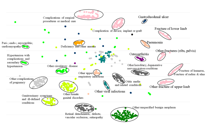
(a) Scatterplot of the final representations $\mathbf{g}_{i}$’s of GRAM+

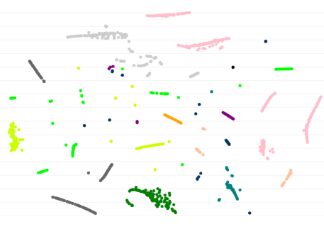
(b) Scatterplot of the final representations $\mathbf{g}_{i}$’s of GRAM

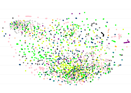
(c) Scatterplot of the trained embedding matrix $\mathbf{W}_{emb}$ of RNN+

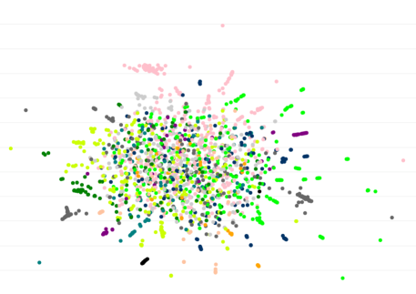
(d) Scatterplot of the trained embedding matrix $\mathbf{W}_{emb}$ of RNN

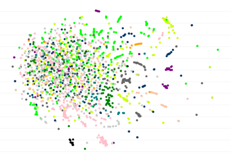
(e) Scatterplot of the final representations $\mathbf{g}_{i}$’s of RandomDAG

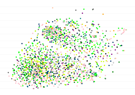
(f) Scatterplot of the disease representations trained by GloVe

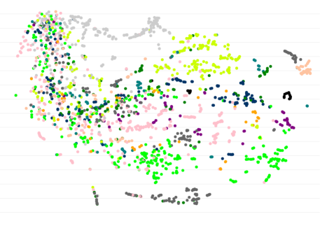
(g) Scatterplot of the basic embeddings $\mathbf{e}_{i}$’s trained by Skip-gram

Figure 3: t-SNE scatterplots of medical concepts trained by GRAM+, GRAM, RNN+, RNN, RandomDAG, GloVe and Skip-gram. The color of the dots represents the highest disease categories and the text annotations represent the detailed disease categories in CCS multi-level hierarchy. It is clear that GRAM+ and GRAM exhibit interpretable embedding that are well aligned with the medical ontology.

representations that are significantly more consistent with the given knowledge DAG $\mathcal{G}$. Based on the prediction performance shown by Table 2, and the fact that the representations $\mathbf{g}_{i}$’s are the final product of GRAM, we can infer that such medically meaningful representations are necessary for predictive models to cope with data insufficiency and make more accurate predictions. Figure 3(b) shows that the quality of the final representations $\mathbf{g}_{i}$ of GRAM is quite similar to GRAM+. Compared to other baselines, GRAM demonstrates significantly more structured representations that align well with the given knowledge DAG. It is interesting that Skip-gram shows the most structured representation among all baselines. We used GloVe to initialize the basic embeddings $\mathbf{e}_{i}$ in this work because it uses global co-occurrence information and its training time is fast as it is only dependent only on the total number of unique concepts $|\mathcal{C}|$. Skip-gram’s training time, on the other hand, depends on both the number of patients and the number of visits each patient made, which makes the algorithm generally slower than GloVe. An interactive visualization tool can be accessed at http://www.sunlab.org/research/gram-graph-based-attention-model/.

3.4 Analysis of the attention behavior

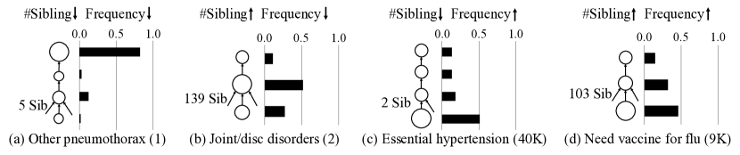
Figure 4: GRAM’s attention behavior during HF prediction for four representative diseases (each column). In each figure, the leaf node represents the disease and upper nodes are its ancestors. The size of the node shows the amount of attention it receives, which is also shown by the bar charts. The number in the parenthesis next to the disease is its frequency in the training data. We exclude the root of the knowledge DAG $\mathcal{G}$ from all figures as it did not play a significant role.

Next we show that GRAM’s attention can be explained intuitively based on the data availability and knowledge DAG’s structure when performing a prediction task. Using Eq. (1), we can calculate the attention weights of individual disease. Figure 4 shows the attention behaviors of four representative diseases when performing HF prediction on Sutter HF cohort.

Other pneumothorax (ICD9 512.89) in Figure 4a is rarely observed in the data and has only five siblings. In this case, most information is derived from the highest ancestor. Temporomandibular joint disorders & articular disc disorder (ICD9 524.63) in Figure 4b is rarely observed but has 139 siblings. In this case, its parent receives a stronger attention because it aggregates sufficient samples from all of its children to learn a more accurate representation. Note that the disease itself also receives a stronger attention to facilitate easier distinction from its large number of siblings.

Unspecified essential hypertension (ICD9 401.9) in Figure 4c is very frequently observed but has only two siblings. In this case, GRAM assigns a very strong attention to the leaf, which is logical because the more you observe a disease, the stronger your confidence becomes. Need for prophylactic vaccination and inoculation against influenza (ICD9 V04.81) in Figure 4d is quite frequently observed and also has 103 siblings. The attention behavior in this case is quite similar to the case with fewer siblings (Figure 4b) with a slight attention shift towards the leaf concept as more observations lead to higher confidence.

4 Related Work

The attention mechanism is a general framework for neural network learning (Bahdanau et al., 2014), and has been since used in many areas such as speech recognition (Chorowski et al., 2014), computer vision (Ba et al., 2014; Xu et al., 2015) and healthcare (Choi et al., 2016b). However, no one has designed attention model based on knowledge ontology, which is the focus of this work.

There are related works in learning the representations of graphs. Several studies focused on learning the representations of graph vertices by using the neighbor information. DeepWalk (Perozzi et al., 2014) and node2vec (Grover and Leskovec, 2016) use random walk while LINE (Tang et al., 2015) uses breadth-first search to find the neighbors of a vertex and learn its representation based on the neighbor information. Graph convolutional approaches (Yang et al., 2016; Kipf and Welling, 2016) also focus on learning the vertex representations to mainly perform vertex classification. All those works focus on solving the graph data problems whereas GRAM focuses on solving clinical predictive modeling problems using the knowledge DAG as supplementary information.

Several researchers tried to model the knowledge DAG such as WordNet (Miller, 1995) or Freebase (Bollacker et al., 2008) where two entities are connected with various types of relation, forming a set of triples. They aim to project entities and relations (Bordes et al., 2013; Socher et al., 2013; Wang et al., 2014; Lin et al., 2015) to the latent space based on the triples or additional information such as hierarchy of entities (Xie et al., 2016). These works demonstrated tasks such as link prediction, triple classification or entity classification using the learned representations. More recently, Li et al. (2016) learned the representations of words and Wikipedia categories by utilizing the hierarchy of Wikipedia categories. GRAM is fundamentally different from the above studies in that it aims to design intuitive attention mechanism on the knowledge DAG as a knowledge prior to cope with data insufficiency and learn medically interpretable representations to make accurate predictions.

A classical approach for incorporating side information in the predictive models is to use graph Laplacian regularization (Weinberger et al., 2006; Che et al., 2015). However, using this approach is not straightforward as it relies on the appropriate definition of distance on graphs which is often unavailable.

5 Conclusion

Data insufficiency, either due to less common diseases or small datasets, is one of the key hurdles in healthcare analytics, especially when we apply deep neural networks models. To overcome this challenge, we leverage the knowledge DAG, which provides a multi-resolution view of medical concepts. We propose GRAM, a graph-based attention model using both a knowledge DAG and EHR to learn an accurate and interpretable representations for medical concepts. GRAM chooses a weighted average of ancestors of a medical concept and train the entire process with a predictive model in an end-to-end fashion. We conducted three predictive modeling experiments on real EHR datasets and showed significant improvement in the prediction performance, especially on low-frequency diseases and small datasets. Analysis of the attention behavior provided intuitive insight of GRAM.

References

- (1)
- Ba et al. (2014) Jimmy Ba, Volodymyr Mnih, and Koray Kavukcuoglu. 2014. Multiple object recognition with visual attention. arXiv:1412.7755 (2014).
- Bahdanau et al. (2014) Dzmitry Bahdanau, Kyunghyun Cho, and Yoshua Bengio. 2014. Neural Machine Translation by Jointly Learning to Align and Translate. arXiv:1409.0473 (2014).
- Bengio et al. (1994) Yoshua Bengio, Patrice Simard, and Paolo Frasconi. 1994. Learning long-term dependencies with gradient descent is difficult. IEEE Transactions on Neural Networks 5, 2 (1994).
- Bollacker et al. (2008) Kurt Bollacker, Colin Evans, Praveen Paritosh, Tim Sturge, and Jamie Taylor. 2008. Freebase: a collaboratively created graph database for structuring human knowledge. In SIGMOD.
- Bordes et al. (2013) Antoine Bordes, Nicolas Usunier, Alberto Garcia-Duran, Jason Weston, and Oksana Yakhnenko. 2013. Translating embeddings for modeling multi-relational data. In NIPS.
- Che et al. (2015) Zhengping Che, David Kale, Wenzhe Li, Mohammad Taha Bahadori, and Yan Liu. 2015. Deep Computational Phenotyping. In SIGKDD.
- Che et al. (2016) Zhengping Che, Sanjay Purushotham, Kyunghyun Cho, David Sontag, and Yan Liu. 2016. Recurrent Neural Networks for Multivariate Time Series with Missing Values. arXiv:1606.01865 (2016).
- Cho et al. (2014) Kyunghyun Cho, Bart Van Merriënboer, Caglar Gulcehre, Dzmitry Bahdanau, Fethi Bougares, Holger Schwenk, and Yoshua Bengio. 2014. Learning phrase representations using RNN encoder-decoder for statistical machine translation. In EMNLP.
- Choi et al. (2016a) Edward Choi, Mohammad Taha Bahadori, Andy Schuetz, Walter F. Stewart, and Jimeng Sun. 2016a. Doctor AI: Predicting Clinical Events via Recurrent Neural Networks. In MLHC.
- Choi et al. (2016b) Edward Choi, Mohammad Taha Bahadori, Andy Schuetz, Walter F. Stewart, and Jimeng Sun. 2016b. RETAIN: Interpretable Predictive Model in Healthcare using Reverse Time Attention Mechanism. In NIPS.
- Choi et al. (2016c) Edward Choi, Mohammad Taha Bahadori, Elizabeth Searles, Catherine Coffey, Michael Thompson, James Bost, Javier T Sojo, and Jimeng Sun. 2016c. Multi-layer Representation Learning for Medical Concepts. In SIGKDD.
- Choi et al. (2016e) Edward Choi, Andy Schuetz, Walter F. Stewart, and Jimeng Sun. 2016e. Using Recurrent Neural Network Models for Early Detection of Heart Failure Onset. Journal of the American Medical Informatics Association (2016), ocw112.
- Choi et al. (2016d) Youngduck Choi, Chill Yi-I Chiu, and David Sontag. 2016d. Learning Low-Dimensional Representations of Medical Concepts. (2016). AMIA CRI.
- Chorowski et al. (2014) Jan Chorowski, Dzmitry Bahdanau, Kyunghyun Cho, and Yoshua Bengio. 2014. End-to-end continuous speech recognition using attention-based recurrent NN: First results. arXiv:1412.1602 (2014).
- Goldberger et al. (2000) Ary Goldberger and others. 2000. Physiobank, physiotoolkit, and physionet components of a new research resource for complex physiologic signals. Circulation (2000).
- Grover and Leskovec (2016) Aditya Grover and Jure Leskovec. 2016. Node2Vec: Scalable Feature Learning for Networks. In SIGKDD.
- Gurwitz et al. (2013) Jerry Gurwitz, David Magid, David Smith, Robert Goldberg, David McManus, Larry Allen, Jane Saczynski, Micah Thorp, Grace Hsu, Sue Hee Sung, and others. 2013. Contemporary prevalence and correlates of incident heart failure with preserved ejection fraction. The American journal of medicine 126, 5 (2013).
- Hochreiter and Schmidhuber (1997) Sepp Hochreiter and Jürgen Schmidhuber. 1997. Long short-term memory. Neural Computation 9, 8 (1997).
- Johnson et al. (2016) Alistair Johnson and others. 2016. MIMIC-III, a freely accessible critical care database. Scientific Data 3 (2016).
- Kipf and Welling (2016) Thomas N Kipf and Max Welling. 2016. Semi-supervised classification with graph convolutional networks. arXiv:1609.02907 (2016).
- Le et al. (2015) Quoc V Le, Navdeep Jaitly, and Geoffrey E Hinton. 2015. A Simple Way to Initialize Recurrent Networks of Rectified Linear Units. arXiv:1504.00941 (2015).
- Li et al. (2016) Yuezhang Li, Ronghuo Zheng, Tian Tian, Zhiting Hu, Rahul Iyer, and Katia Sycara. 2016. Joint Embedding of Hierarchical Categories and Entities for Concept Categorization and Dataless Classification. (2016).
- Lin et al. (2015) Yankai Lin, Zhiyuan Liu, Maosong Sun, Yang Liu, and Xuan Zhu. 2015. Learning Entity and Relation Embeddings for Knowledge Graph Completion. In AAAI.
- Lipton et al. (2015) Zachary C Lipton, David C Kale, Charles Elkan, and Randall Wetzell. 2015. Learning to Diagnose with LSTM Recurrent Neural Networks. arXiv:1511.03677 (2015).
- Lipton et al. (2016) Zachary C Lipton, David C Kale, and Randall Wetzel. 2016. Modeling Missing Data in Clinical Time Series with RNNs. In MLHC.
- Maaten and Hinton (2008) Laurens van der Maaten and Geoffrey Hinton. 2008. Visualizing data using t-SNE. JMLR 9, Nov (2008).
- Mikolov et al. (2013) Tomas Mikolov, Ilya Sutskever, Kai Chen, Greg Corrado, and Jeff Dean. 2013. Distributed representations of words and phrases and their compositionality. In NIPS.
- Miller (1995) George A Miller. 1995. WordNet: a lexical database for English. Commun. ACM 38, 11 (1995).
- Miotto et al. (2016) Riccardo Miotto, Li Li, Brian A Kidd, and Joel T Dudley. 2016. Deep Patient: An Unsupervised Representation to Predict the Future of Patients from the Electronic Health Records. Scientific Reports 6 (2016).
- Nguyen et al. (2016) Phuoc Nguyen, Truyen Tran, Nilmini Wickramasinghe, and Svetha Venkatesh. 2016. Deepr: A Convolutional Net for Medical Records. arXiv:1607.07519 (2016).
- Pennington et al. (2014) Jeffrey Pennington, Richard Socher, and Christopher D Manning. 2014. Glove: Global Vectors for Word Representation. In EMNLP.
- Perozzi et al. (2014) Bryan Perozzi, Rami Al-Rfou, and Steven Skiena. 2014. DeepWalk: Online Learning of Social Representations. In SIGKDD.
- Project et al. (2010) Healthcare Cost & Utilization Project and others. 2010. Clinical classifications software (CCS) for ICD-9-CM. Rockville, MD: Agency for Healthcare Research and Quality (2010).
- Razavian et al. (2016) Narges Razavian, Jake Marcus, and David Sontag. 2016. Multi-task Prediction of Disease Onsets from Longitudinal Lab Tests. In MLHC.
- Socher et al. (2013) Richard Socher, Danqi Chen, Christopher D Manning, and Andrew Ng. 2013. Reasoning with neural tensor networks for knowledge base completion. In NIPS.
- Stearns et al. (2001) Michael Q Stearns, Colin Price, Kent A Spackman, and Amy Y Wang. 2001. SNOMED clinical terms: overview of the development process and project status. In AMIA.
- Tang et al. (2015) Jian Tang, Meng Qu, Mingzhe Wang, Ming Zhang, Jun Yan, and Qiaozhu Mei. 2015. LINE: Large-scale Information Network Embedding. In WWW.
- Team (2016) The Theano Development Team. 2016. Theano: A Python framework for fast computation of mathematical expressions. arXiv:1605.02688 (2016).
- Vijayakrishnan et al. (2014) Rajakrishnan Vijayakrishnan, Steven Steinhubl, Kenney Ng, Jimeng Sun, Roy Byrd, Zahra Daar, Brent Williams, Shahram Ebadollahi, Walter Stewart, and others. 2014. Prevalence of heart failure signs and symptoms in a large primary care population identified through the use of text and data mining of the electronic health record. Journal of cardiac failure 20, 7 (2014).
- Wang et al. (2014) Zhen Wang, Jianwen Zhang, Jianlin Feng, and Zheng Chen. 2014. Knowledge Graph Embedding by Translating on Hyperplanes. In AAAI.
- Weinberger et al. (2006) Kilian Q Weinberger, Fei Sha, Qihui Zhu, and Lawrence K Saul. 2006. Graph Laplacian Regularization for Large-Scale Semidefinite Programming. In NIPS.
- Xie et al. (2016) Ruobing Xie, Zhiyuan Liu, and Maosong Sun. 2016. Representation Learning of Knowledge Graphs with Hierarchical Types. In IJCAI.
- Xu et al. (2015) Kelvin Xu, Jimmy Ba, Ryan Kiros, Kyunghyun Cho, Aaron Courville, Ruslan Salakhutdinov, Richard Zemel, and Yoshua Bengio. 2015. Show, Attend and Tell: Neural Image Caption Generation with Visual Attention.. In ICML.
- Yang et al. (2016) Zhilin Yang, William Cohen, and Ruslan Salakhutdinov. 2016. Revisiting Semi-Supervised Learning with Graph Embeddings. arXiv:1603.08861 (2016).
- Zeiler (2012) Matthew D Zeiler. 2012. ADADELTA: an adaptive learning rate method. arXiv:1212.5701 (2012).