Experimental and theoretical oscillator strengths of Mg I for accurate abundance analysis

Abstract

Context. With the aid of stellar abundance analysis, it is possible to study the galactic formation and evolution. Magnesium is an important element to trace the $\alpha$-element evolution in our Galaxy. For chemical abundance analysis, such as magnesium abundance, accurate and complete atomic data are essential. Inaccurate atomic data lead to uncertain abundances and prevent discrimination between different evolution models.

Aims. We study the spectrum of neutral magnesium from laboratory measurements and theoretical calculations. Our aim is to improve the oscillator strengths ($f$-values) of Mg I lines and to create a complete set of accurate atomic data, particularly for the near-IR region.

Methods. We derived oscillator strengths by combining the experimental branching fractions with radiative lifetimes reported in the literature and computed in this work. A hollow cathode discharge lamp was used to produce free atoms in the plasma and a Fourier transform spectrometer recorded the intensity-calibrated high-resolution spectra. In addition, we performed theoretical calculations using the multiconfiguration Hartree-Fock program ATSP2K.

Results. This project provides a set of experimental and theoretical oscillator strengths. We derived 34 experimental oscillator strengths. Except from the Mg I optical triplet lines (3p ³P${}^{o}_{0,1,2}$ - 4s ³S₁), these oscillator strengths are measured for the first time. The theoretical oscillator strengths are in very good agreement with the experimental data and complement the missing transitions of the experimental data up to $n=7$ from even and odd parity terms. We present an evaluated set of oscillator strengths, gf, with uncertainties as small as 5%. The new values of the Mg I optical triplet line (3p ³P${}^{o}_{0,1,2}$ - 4s ³S₁) oscillator strength values are $\sim$0.08 dex larger than the previous measurements.

1 Introduction

Magnesium is an important element for chemical evolution studies. It is an $\alpha$-element, which is formed and released during supernova type II explosions of massive stars. Magnesium lines are strong in the spectra of late-type stars and even in metal-poor stars. Therefore, it is an ideal element to trace the $\alpha$-element abundances.
The dominant electron source in the stellar atmospheres of metal-poor stars is magnesium. As a result, its abundance affects the model atmospheres (Prochaska et al., 2000). The higher the magnesium abundance, the higher the electron density becomes in the stellar atmosphere. Neglecting this fact may lead to incorrect stellar gravity determination. Prochaska et al. (2000) used an $\alpha$-enhanced model atmosphere to derive abundances. For magnesium abundance analysis, they only found very few magnesium lines with reported $\log(gf)$ values. Because of the missing data, they included additional lines with astrophysical $\log(gf)$ values.
Several studies (Shigeyama & Tsujimoto, 1998; Bensby et al., 2003; Cayrel et al., 2004; Andrievsky et al., 2010) have used magnesium as an alternative to iron for tracing the chemical evolution of the Milky Way. Magnesium is only formed in supernova type II explosions of massive stars (Woosley & Weaver, 1995), whereas iron has several formation channels (Thielemann et al., 2002). A complete set of magnesium atomic data results in more accurate abundances and, correspondingly, makes magnesium an even better choice as a tracer of galactic evolution.
At temperatures $T\geq 5000K$, magnesium is primarily singly ionised. However there are a large number of Mg I lines existing in the solar spectrum (Scott et al., 2015). As a result of Mg⁺ being the dominant species, Mg I is sensitive to the deviations from local thermodynamic equilibrium (LTE). In particular, for the metal-poor stars, these non-LTE effects are predicted to be significant (Zhao et al., 1998; Zhao & Gehren, 2000). To study the deviations from LTE, It is crucial to have accurate atomic data of both Mg I and Mg II. This makes it possible to map the limits of LTE approximations as a function of stellar metallicity, gravity, and temperature, similar to Fe I in Lind et al. (2012). There are several studies on NLTE analysis of neutral magnesium including the recent studies of Bergemann et al. (2015); Osorio & Barklem (2016).The former studied NLTE effects in the J-band Mg I lines and due to a lack of experimental $\log(gf)$ values, calculated $\log(gf)$ values were used. However, using the average of the many calculated $\log(gf)$ values overestimated the line depths, Bergemann et al. (2015) concluded that the values were wrong and derived their astrophysical $\log(gf)$ values.
Scott et al. (2015) determined the magnesium abundance of the Sun to be $\log\epsilon_{\text{Mg}}=7.59\pm 0.04$ from a 3D hydrodynamic model of the solar photosphere. However, due to the lack of laboratory measurements of $\log(gf)$ values, they used theoretical $\log(gf)$ values of Butler et al. (1993) and Chang & Tang (1990). The current study provides experimental $\log(gf)$ values for two of the lines and improved theoretical $\log(gf)$ values for all the lines used by Scott et al. (2015).
In addition, some planetary atmosphere studies show the presence of magnesium in the atmospheres of planets (Fossati et al., 2010; Vidal-Madjar et al., 2013; Bourrier et al., 2014, 2015). By analysing the resonance line of an abundant element, such as magnesium, during a planet transit, the atmospheric escape mechanism can be understood. These studies are usually done by analysing absorption depths of the line of interest, which requires accurate atomic data.
To our knowledge there are no experimental oscillator strengths of Mg I lines, except from the $3\text{s}^{2}$ ${}^{1}\text{S}_{0}-3\text{s}3\text{p}$ ${}^{3}\text{P}_{1}$ intercombination transition at 4571 $\AA$ (Kwong et al., 1982) and the Mg I triplets lines (3p ³P${}^{o}_{0,1,2}$ - 4s ³S₁); 5167, 5172, and 5183 $\AA$ (Aldenius et al., 2007). Although Ueda et al. (1982) provided oscillator strengths for the transitions from 3p ³P level, they were not completely experimental values. Theoretical calculations in Wiese et al. (1969) compilation were used for the absolute scale of the oscillator strengths.
There are several theoretical values, which are generally used for abundance analysis. Chang & Tang (1990) calculated oscillator strengths of Mg I lines between selected ^1,3S - ^1,3F states using the configuration interaction (CI) procedure with a finite basis set constructed from B splines. In addition, theoretical values of Butler et al. (1993) are commonly used for abundance analyses. They used the close-coupling approximation with the R-matrix technique. Moreover, Civiš et al. (2013) performed oscillator strength calculations using the quantum defect theory (QDT) in the region of $800-9000$ cm^-1. Froese Fischer et al. (2006) performed calculations using the multi configuration Hartree-Fock method. Their calculations included the terms up to $n=4$ and all three types of correlations: valence, core-valence, and core-core correlation.
This paper presents experimental $\log(gf)$ values of Mg I lines from high-resolution laboratory measurements in the infrared and optical region from the upper even parity 4s ^1,3S, 5s ¹S, 3d ¹D, and 4d ¹D terms and the odd parity 4p ³P^o, 5p ³P^o, 4f ^1,3F^o, and 5f ^1,3F^o terms. In addition, we performed multiconfiguration Hartree-Fock calculations using the ASTP2K package (Froese Fischer et al., 2007) and obtained $\log(gf)$ values of Mg I lines up to $n=7$ from even parity ^1,3S, ^1,3D, and^1,3G terms and odd parity ^1,3P^o, and ^1,3F^o terms. The transitions between the higher terms fall in the IR spectral region and the calculated $\log(gf)$ values are important for interpreting observations using the new generation of telescopes designed for this region. Following the introduction, Sect. 2 describes the experimental method we used for deriving $\log(gf)$ values. In addition, this section explains the measurements of branching fractions ($BF$) and the uncertainty estimations. The theoretical calculations that we performed are explained in Sect. 3. In Sect. 4, we present our results, the comparisons of our results with previous studies, and the conclusions.

2 Experimental method

We used a water-cooled hollow cathode discharge lamp (HCL) with a magnesium cathode as a light source to produce the magnesium plasma. The experimental set-up was similar to the one described by Pehlivan et al. (2015). The strongest lines for the measurements were obtained using neon as carrier gas and with an applied current of $0.60$ A.
We recorded the Mg I spectra with the high-resolution Fourier transform spectrometer (FTS), Bruker IFS 125 HR, at the Lund Observatory (Edlén Laboratory). The maximum resolving power of the instrument is $10^{6}$ at 2000 cm^-1 and the covered wavenumber region is $50000-2000$ cm^-1 ($200-5000$ nm). We set the resolution to $0.01$ cm^-1 during the measurements and recorded the spectra with indium antimonide (InSb), silicon (Si), and photomultiplier tube (PMT) detectors. These detectors are sensitive to different spectral regions, but they overlap each other in a small wavelength region.
The optical element contributions to the FTS response function were compensated for by obtaining an intensity calibration. Because of the wavelength-dependent transmission of the optical elements and the spectrometer, the measured intensities of the lines differ from their intrinsic intensities. Therefore, we acquired the response function of the instrument for three different detectors that we used during different measurements. The response function is usually determined by measuring the spectrum of an intensity calibrated reference lamp. We used a tungsten filament lamp for the intensity calibration of Mg I lines. The lamp was calibrated by the Swedish National Laboratory (SP) for spectral radiance in the region between $40000-4000$ cm^-1 ($250-2500$ nm). With the calibrated radiance of the lamp, the response function of the instrument can be determined for different detectors. We used the overlapping region Mg I lines, which were recorded with different detectors, to connect the relative intensities on the same scale. This was done by using a normalisation factor $nf$, which in turn contributed an additional uncertainty to the $BF$s.
In addition, we recorded the spectra with different currents to compensate for self-absorption effects. The self-absorption affects the intensity of the line and this, in turn, influences the BF measurements which are used to determine the oscillator strengths. More details can be found in our previous paper (Pehlivan et al., 2015).

2.1 Branching fraction measurements

The oscillator strength of a spectral line is proportional to the transition probability. For electric dipole transition, it is given as

$$f=\frac{g_{\text{u}}}{g_{\text{l}}}\lambda^{2}A_{\text{ul}}1.499\times 10^{-16},$$ (1)

where $g_{\text{u}}$ is the statistical weight of the upper level, $g_{\text{l}}$ the statistical weight of the lower level, $\lambda$ the wavelength of the transition in Å, and $A_{\text{ul}}$ the transition probability between the upper level u and the lower level l in s^-1.
The radiative lifetime of an upper level, $\tau_{\text{u}}$ is the inverse of the sum of all transition probabilities from the same upper level, $\tau_{\text{u}}=1/\sum_{i}A_{\text{u}i}$. The branching fraction (BF) of a line is defined as the transition probability of the line $A_{\text{ul}}$ divided by the total transition probability of the lines from the same upper level;

$$BF_{\text{ul}}=\frac{A_{\text{ul}}}{\sum_{\rm i}A_{\text{u}i}}=\frac{I_{\text{ul}}}{\sum_{\rm i}I_{\text{u}i}}.$$ (2)

As the transition probability is proportional to the line intensity $I_{\text{ul}}$, $BF$ can be defined as the ratio of the line intensities.
Knowing the radiative lifetime and combining this with the measured $BF$s, one can derive the transition probability, $A_{\text{ul}}$, of a spectral line;

$$A_{\text{ul}}=\frac{BF_{\text{ul}}}{\tau_{\text{u}}}.$$ (3)

Transitions from the same upper level can have wavelengths belonging to different regions of the electromagnetic spectrum. However, to accurately measure $BF$s, all transitions from the same upper level should be accounted for. For this reason, we recorded Mg I spectra using different detectors. These different spectra were put on the same relative intensity scale by using a normalisation factor.

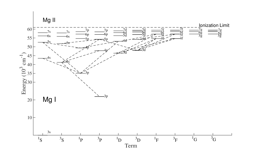
Figure 1: Partial energy level diagram of Mg I with dashed lines showing the observed transitions. The energy level values are from Martin & Zalubas (1980).

A partial energy level diagram of Mg I levels is shown in Fig. 1. The transitions, which we observed and used to derive $\log(gf)$ values, are marked in this figure. Using the Kurucz (2009) database and references in Kaufman & Martin (1991), we predicted the Mg I lines from the same upper level. We identified these lines and analysed our recorded spectra with the FTS analysis software GFit (Engström, 1998, 2014).
Mg I has three dominant isotopes: $\@element[24]{\mathrm{Mg}}$ with 78.99% abundance, $\@element[25]{\mathrm{Mg}}$ with 10% abundance, and $\@element[26]{\mathrm{Mg}}$ with 11% abundance (IUPAC 1991). Although there are three isotopes of Mg I, in our measurements we did not see any isotope shift. The nuclear spins of these isotopes are $0$, $5/2$, and $0$, respectively. This proves that the most dominant isotope $\@element[24]{\mathrm{Mg}}$ has no hyperfine splitting (hfs) in the line profiles. Even though $\@element[25]{\mathrm{Mg}}$ has a nuclear spin of $5/2$, we did not see any hfs as the abundance of this isotope is very low compared to $\@element[24]{\mathrm{Mg}}$.

2.2 Uncertainties

The uncertainty of the $BF$ contains several components. Together with the uncertainty of the intensities, the uncertainty of the self-absorption correction, the uncertainty of the intensity calibration lamp, and the uncertainty of the normalisation factor, which is used to put the intensities on the same scale, should be considered. Including all of these uncertainty components, Sikström et al. (2002) defined the total uncertainty of the $BF$ as,

$$\Bigg{(}\frac{u(BF)}{BF}\Bigg{)}^{2} =(1-(BF)_{k})^{2}\hskip 1.70717pt\Bigg{(}\frac{u(I_{k})}{I_{k}}\Bigg{)}^{2}$$

$$+\sum\limits_{j\neq k(inP)}(BF)_{j}^{2}\hskip 2.27621pt\Bigg{(}\bigg{(}\frac{u(I_{j})}{I_{j}}\bigg{)}^{2}+\bigg{(}\frac{u(c_{j})}{c_{j}}\bigg{)}^{2}\Bigg{)}$$

$$+\sum\limits_{j\neq k(inQ)}(BF)_{j}^{2}\hskip 2.27621pt\Bigg{(}\bigg{(}\frac{u(I_{j})}{I_{j}}\bigg{)}^{2}+\bigg{(}\frac{u(c_{j})}{c_{j}}\bigg{)}^{2}+\bigg{(}\frac{u(nf)}{nf}\bigg{)}^{2}\Bigg{)}.$$ (4)

The first term of the equation includes the branching fraction $(BF)_{k}$ of the line of interest in the spectral region of the detector $P$ and the uncertainty in the measured intensity of the same line, $u(I_{k})$. In the sum that follows $u(c_{j})$ and $u(I_{j})$ are the uncertainties of the calibration lamp and the uncertainties of the measured intensities, respectively, for other lines from the same upper level recorded with the detector P. $(BF)_{j}$ are the branching fractions. The last sum, that describes uncertainties from lines recorded with detector Q, also includes the uncertainty $u(nf)$ in the normalisation factor $nf$ connecting different spectral regions. The intensity uncertainties from the statistical noise were determined using GFit. They varied between $0.001\%$ for the strong lines and $\sim 20\%$ for the weak lines or self-absorbed lines. Most of the lines have uncertainties below $1\%$. When there was self-absorption, we corrected these lines and added the uncertainty from self-absorption to the intensity uncertainty. The calibration lamp uncertainty is $7\%$ and the uncertainty of the normalisation factor is $5\%$. From propagation of errors and using Eq. (3), the uncertainty of the transition probability or $f$-value is defined as,

$$\Bigg{(}\frac{u(f_{k})}{f_{k}}\Bigg{)}^{2}=\Bigg{(}\frac{u(A_{k})}{A_{k}}\Bigg{)}^{2}=\Bigg{(}\frac{u(BF)}{BF}\Bigg{)}^{2}+\Bigg{(}\frac{u(\tau)}{\tau}\Bigg{)}^{2},$$ (5)

where $u(\tau)$ is the uncertainty of the radiative lifetime of the upper level. In the cases where we used experimental lifetimes of Jönsson et al. (1984), the uncertainties vary between $5\%$ and $7\%$. For the theoretical lifetime uncertainties, we compared our theoretical values (to be described in the following section) with the experimental lifetimes available in the literature (Kwiatkowski et al., 1980; Jönsson et al., 1984; Larsson & Svanberg, 1993; Larsson et al., 1993; Aldenius et al., 2007). Figure 2 shows the comparison of the experimental lifetime values with the theoretical lifetime values that we calculated. The blue dashed line marks the $15\%$ and the black dashed line marks the $10\%$ difference. As the difference is small, we adopted $10\%$ relative uncertainty for the theoretical lifetimes.

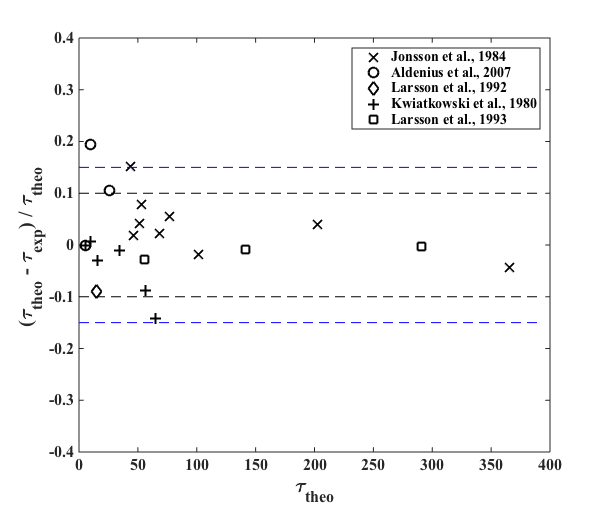
Figure 2: Comparison of the theoretical lifetimes of this study with the previously measured experimental lifetimes. As seen in the figure, there is a large difference of almost $20\%$ for one of the values measured by Aldenius et al. (2007). However, a re-measurement of the lifetime brings it in a very good agreement with the calculated value (see text for more details).

3 Theoretical method

We performed our calculations using the multiconfiguration Hartree-Fock method (MCHF) (Froese Fischer et al., 1997, 2016). In this method , atomic state functions (ASF) $\Psi(\gamma LS)$ for the $LS$ terms are represented by linear combinations of configuration state functions (CSF);

$$\Psi(\gamma LS)=\sum\limits_{i}c_{i}\Phi(\gamma_{i}LS).$$ (6)

In the equation, $\gamma$ represents the electronic configurations and the quantum numbers other than $L$ and $S$. The configuration state functions $\Phi(\gamma_{i}LS)$ are built from one-electron orbitals and $c_{i}$ are the mixing coefficients. The mixing coefficients and the radial parts of the one-electron orbitals are determined by solving a set of equations that results from applying the variational principle to the energy expression associated with the ASFs.
We started with a calculation of the ASFs describing terms of the configurations with $n$ up to nine and $l$ up to $g$ such as 3s², 3s3p, 3s3d, …3s9g. The calculation was done in the simplest approximation, where each ASF consists of only one CSF. All the ASFs were determined together in the same run and the calculation yielded a number of orbitals that were kept fixed in the proceeding calculations.
Terms involving configurations with $n=8,9$ were not our prime target. However, we included these terms in the initial calculation to obtain orbitals that are spatially localised far away from the nucleus. This leads to a more complete and balanced orbital set. To improve the ASFs describing terms of the configurations with $n$ up to seven and $l$ up to $g$, such as 3s², 3s3p, 3s3d, …3s7g, we performed calculations with systematically enlarged CSF expansions. These expansions were formed from single and double replacements of orbitals in the reference configurations with orbitals in an active orbital set. We applied restrictions that there should be at most one replacement from 2s²2p⁶ and 1s² should be a closed shell. The orbitals in the active set were extended to include orbitals with $n=13$ and $l=h$. In these calculations, we determined ASFs with the same $LS$ symmetry together.
Once the ASFs were determined, the oscillator strengths were calculated as expectation values of the transition operator. We performed the calculations both in the length and in the velocity gauge; see Froese Fischer et al. (1997) for more details. For accurate calculations, the oscillator strengths in the two gauges should give the same value. In our calculations, the oscillator strengths in the two gauges typically agree to within $5\%$ for transitions between low-lying terms. The agreement is slightly worse for transitions involving the highest terms. Nevertheless, the velocity gauge, which weights more to the inner part of the wave function, shows good convergence properties and is believed to be the more accurate one for transitions involving the more excited states.
All calculations were non-relativistic and the obtained $gf$ values represent term averages. To obtain the $gf$ values for the fine-structure transitions rather than for transitions between terms, we multiplied the $gf$ values for the term averages with the square of the line factor, see Cowan (1981) Eq. (14.50).
Moreover, we investigated the influence of relativistic effects by comparing our results with results from calculations where relativistic effects were accounted for in the Breit-Pauli approximation. As expected, the relativistic effects were insignificant with negligible term mixing. Exceptions are the $J=3$ states of the ^1,3F terms in which the energy separations are so small that even weak relativistic effects give considerable term mixing. For the states of 4f ^1,3F terms, we performed full calculations with relativistic effects in the Breit-Pauli method and applied the method of fine tuning (Brage & Hibbert, 1989) to match with the experimental data of Martin & Zalubas (1980). Due to the very small energy separations, it was not possible to perform these calculations for the higher $n$ and thus no theoretical oscillator strength values are given for states of the 5f, 6f, 7f ^1,3F terms.

4 Results and conclusions

In this study, experimental and theoretical oscillator strengths of Mg I are provided. $BF$s were obtained using Eq. 2 from the observed line intensities. We recorded the spectra using different currents and detectors. Applying different currents helped to rule out any self-absorption effects. The spectra, which are recorded with different detectors, are put on the same intensity scale by using a normalisation factor. In this way, we had all the lines from the same upper level on the same intensity scale. In the cases where we had unobservable weak lines, we used the theoretical transition probabilities to estimate the residual values.
From the measured $BF$s and radiative lifetimes, the transition probabilities, $A_{ul}$, are derived using Eq. 3 and $\log(gf)$ values are derived from Eq. 1. For the experimental lifetimes, we used the values of Jönsson et al. (1984), and for others, we used our theoretical radiative lifetimes. Table 1 shows the theoretical lifetime values we computed together with the previous experimental and theoretical lifetime values. One notes that sometimes there are very large differences between values by Kurucz (2009) and the experimental values.

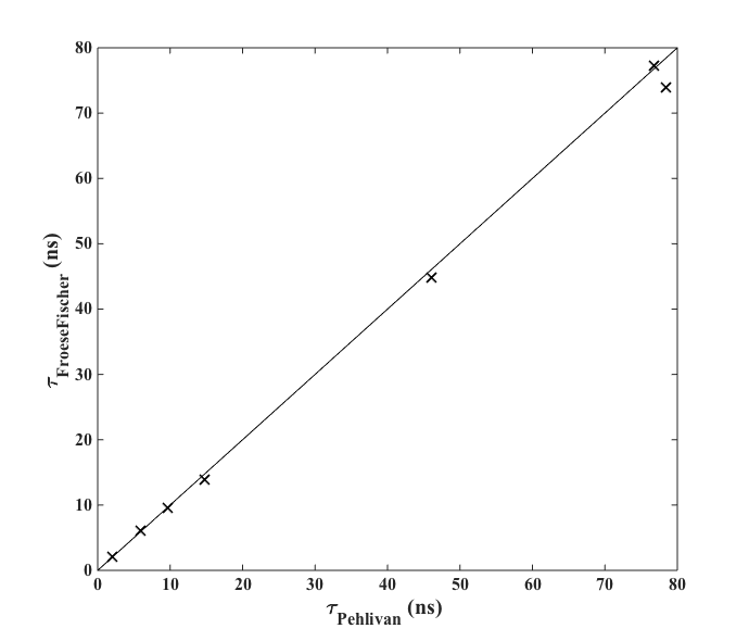
Figure 3: Comparison between lifetime values of Froese Fischer et al. (2006) and this work.

Figure 4: Comparison between experimental and theoretical log$(gf)$ values of this work. The theoretical and experimental $\log(gf)$ values differ markedly for two transitions. These two transitions are affected by a blend and thus the derived experimental values are very uncertain (see text for more details).

Table 1: Theoretical radiative lifetimes of this work together with previous theoretical and experimental lifetimes.

Level	Calculations (ns)			Experimental (ns)
	This work	K091	CFF062	KW803	J844	LS935	L936	A077
3s3p 1Po	2. 1	1.7	2.1	-	-	-	-	-
3s4s 3S	9.6	7.6	9.6	9.7(6)	-	-	-	11.5(1.0)
3s4s 1S	46	35	44.8	-	47(3)	-	-	-
3s3d 1D	77	53	77.2	-	81(6)	-	-	-
3s4p 3Po	79	69	73.9	-	-	-	-	-
3s3d 3D	5.9	4.7	6.0	5.9(4)	-	-	-	5.9(4)
3s4p 1Po	14.7	16.8	13.8	-	-	13.4(4)	-	-
3s5s 3S	26	28	-	-	-	-	-	29(3)
3s5s 1S	102	65	-	-	100(5)	-	-	-
3s4d 1D	53	64	-	-	57(3)	-	-	-
3s4d 3D	16.1	13.7	-	15.6(9)	-	-	-	17.6(1.2)
3s5p 3Po	268	211	-	-	-	-	-	-
3s4f 1Fo	61	41	-	-	-	-	-	-
3s4f 3Fo	61	48	-	-	-	-	-	-
3s5p 1Po	56	98	-	-	-	-	54(3)	-
3s6s 3S	57	63	-	51.8(3.0)	-	-	-	-
3s6s 1S	203	112	-	-	211(12)	-	-	-
3s5d 1D	43	56	-	-	50(4)	-	-	-
3s5d 3D	35	33	-	34.1(1.5)	-	-	-	33(3)
3s6p 3Po	642	502	-	-	-	-	-	-
3s5f 1Fo	121	89	-	-	-	-	-	-
3s5f 3Fo	119	102	-	-	-	-	-	-
3s6p 1Po	141	348	-	-	-	-	140(10)	-
3s5g 3G	226	211	-	-	-	-	-	-
3s5g 1G	226	211	-	-	-	-	-	-
3s7s 3S	109	117	-	-	-	-	-	-
3s7s 1S	366	181	-	-	350(16)	-	-	-
3s6d 1D	52	77	-	-	54(3)	-	-	-
3s6d 3D	65	68	-	55.7(3.0)	-	-	-	-
3s7p 3Po	1280	990	-	-	-	-	-	-
3s6f 1Fo	216	165	-	-	-	-	-	-
3s6f 3Fo	209	182	-	-	-	-	-	-
3s7p 1Po	291	752	-	-	-	-	290(20)	-
3s6g 3G	387	365	-	-	-	-	-	-
3s6g 1G	387	365	-	-	-	-	-	-
3s7d 1D	69	120	-	-	70(6)	-	-	-
3s7d 3D	113	126	-	91.5(5.0)	-	-	-	-
3s7f 3Fo	337	296	-	-	-	-	-	-
3s7f 1Fo	355	287	-	-	-	-	-	-
3s7g 3G	610	578	-	-	-	-	-	-
3s7g 1G	610	578	-	-	-	-	-	-

¹Kurucz (2009); ²Froese Fischer et al. (2006); ³Kwiatkowski et al. (1980); ⁴Jönsson et al. (1984); ⁵Larsson & Svanberg (1993); ⁶Larsson et al. (1993); ⁷Aldenius et al. (2007).

Figure 2 shows a comparison of our theoretical lifetime values with experimental work of Kwiatkowski et al. (1980); Jönsson et al. (1984); Larsson & Svanberg (1993); Larsson et al. (1993); Aldenius et al. (2007). Overall, our calculations agree with the previously published experimental values within the 10% uncertainty. Furthermore, we compared our lifetime values with the theoretical values from Froese Fischer et al. (2006) in Fig. 3 and the agreement is very good. Even the largest deviations are less than $6\%$.
From experimental $BF$s, we derived 34 $\log(gf)$ values of Mg I lines from the upper even parity 4s ^1,3S, 5s ¹S, 3d ¹D, and 4d ¹D, and odd parity 4p ³P^o, 5p ³P^o, 4f ^1,3F^o, and 5f ^1,3F^o with uncertainties in gf as low as 5%. In addition, we calculated theoretical $\log(gf)$ values of Mg I lines up to $n=7$ from even parity ^1,3S, ^1,3D, and ^1,3G terms, and odd parity ^1,3P^o and ^1,3F^o terms using ATSP2K package. Figure 4 shows the comparison between the experimental and the theoretical $\log(gf)$ values. The good agreement between our experimental and theoretical $\log(gf)$ values makes us confident to recommend our theoretical values for the transitions in Table 3. Table 2 shows our experimental $\log(gf)$ values together with their uncertainty and corresponding theoretical $\log(gf)$ values that we calculated in this study, together with the branching fractions $BF$ and the transition probabilities $A_{ul}$. In addition, we compared our theoretical $\log(gf)$ values with Froese Fischer et al. (2006) values in Fig. 5. Froese Fischer et al. (2006) performed calculations for only the lowest lying levels up to $n=4$ while the current study calculations are additionally for higher levels up to $n=7$. The good agreement between our values and the theoretical values of Froese Fischer et al. (2006) is an additional indication of the quality of our values. Covering much more states and transitions, our calculations complement those of Froese Fischer et al. (2006).

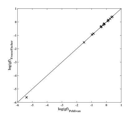
Figure 5: Comparison of $\log(gf)$ values of the current study with the values of Froese Fischer et al. (2006).

Overall, our theoretical lifetime values are in very good agreement with the experimental lifetime values in the literature. In addition, our theoretical $\log(gf)$ values agree with the experimental values of this work. However, our $\log(gf)$ values differ from the Aldenius et al. (2007) values for the optical Mg I triplet lines (3p ³P${}^{o}_{0,1,2}$ - 4s ³S₁), although we measured the same $BF$s. Figure 6(a) shows these lines in one of our spectra. The difference in $\log(gf)$ arises from the radiative lifetime of the upper level. Aldenius et al. (2007) measured the lifetime of $4\text{s}$ ³S₁ level to 11.5$\pm$1.0 ns. Other experimental studies find the lifetime ranging from 5.8 ns to 14.8 ns (Berry et al., 1970; Schaefer, 1971; Andersen et al., 1972; Havey et al., 1977; Kwiatkowski et al., 1980). Apparently, there is a large spread in the literature values and a 2 ns difference in lifetime corresponding to a 0.08 dex difference in log($gf$) values. The derived $\log(gf)$ value is thus sensitive to the choice of lifetime. Using the facility at Lund High Power Laser Centre, we remeasured the lifetime of this level. The atomic structure of Mg I and technical limitations prevented us from deriving a conclusive value. However, the remeasured value leans towards the measurements by Kwiatkowski et al. (1980) and our calculated value. Therefore, we adopted our theoretical lifetime value (9.63 ns) for the $4\text{s}$ ³S₁ level. Our calculated lifetime value of 9.63 ns is a good choice, because it shows internal consistency between the length and velocity gauges, and in comparisons with other levels. Furthermore, Mashonkina (2013) investigated the atomic data used in stellar magnesium abundance analyses. The paper found that the Aldenius et al. (2007) values overestimate the magnesium abundance by 0.11 dex compared to the other lines. With our experimental values this difference will be reduced.
We recommend our experimental oscillator strengths when available. However, we would like to point out that the uncertainties of the Mg I 15886.26 $\AA$ (6293.03 cm^-1) and 15886.18 $\AA$ (6293.06 cm^-1) are larger than 20% owing to the weak line intensities and the blending of these two lines with each other. The oscillator strengths of these lines are outliers in Fig. 4. The lines are displayed in figure 7. It is seen that they are weak with small separations, making fits to line profiles difficult. For these reasons, we advise the use of theoretical values for these transitions. When the experimental data are not available, we suggest theoretical values to be used.

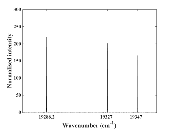
(a)

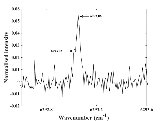
(b)

Figure 6: Sample spectrum of two spectral regions of the FTS recordings. a) The Mg I optical triplet lines (3p ³P${}^{o}_{0,1,2}$ - 4s ³S₁). b) The feature consisting of the 3d ³D_2,1 - 5p ³P${}^{o}_{1}$ transitions.

longtablel c c c c c c c

Transition & $\lambda$ $\sigma$ $BF$ $BF$ Unc. $A_{ul}$ log($gf$) log($gf$)
$(\AA)$ (cm^-1) $\%$ (s^-1) Exp. Calc.

3p ³P${}^{o}_{0}$ - 4s ³S₁ 5167.321 19346.997 0.1121 7 $9.75\times 10^{6}$ -0.854$\pm$0.05 -0.865
3p ³P${}^{o}_{1}$ 5172.684 19326.939 0.3471 3 $3.02\times 10^{7}$ -0.363$\pm$0.04 -0.387
3p ³P${}^{o}_{2}$ 5183.604 19286.225 0.5408 1 $4.70\times 10^{7}$ -0.168$\pm$0.04 -0.166
$Residual$ $<10^{-4}$
$\tau=9.6^{*}$ ns

3p ¹P${}^{o}_{1}$ - 4s ¹S₀ 11828.185 8452.08 1 0 $2.13\times 10^{7}$ -0.350$\pm$0.03 -0.343
$Residual$ $<10^{-4}$
$\tau=47$ ns

3p ¹P${}^{o}_{1}$ - 3d ¹D₂ 8806.756 11351.800 1 0 $1.23\times 10^{7}$ -0.144$\pm$0.03 -0.128
$Residual$ $<10^{-4}$
$\tau=81$ ns

4s ³S₁ - 4p ³P${}^{o}_{0}$ 15047.705 6643.71 1 0 $1.27\times 10^{7}$ -0.364$\pm$0.04 -0.360
$\tau=78.5^{*}$ ns

4s ³S₁ - 4p ³P${}^{o}_{1}$ 15040.246 6647.01 1 0 $1.27\times 10^{7}$ 0.113$\pm$0.04 0.117
$Residual$ $<10^{-4}$
$\tau=78.5^{*}$ ns

4s ³S₁ - 4p ³P${}^{o}_{2}$ 15024.992 6653.76 1 0 $1.27\times 10^{7}$ 0.334$\pm$0.03 0.339
$\tau=78.5^{*}$ ns

3p ¹P${}^{o}_{1}$ - 5s ¹S₀ 5711.088 17504.942 0.2942 10 $2.94\times 10^{6}$ -1.842$\pm$0.05 -1.742
4p ¹P${}^{o}_{1}$ 31157.72^vac 3209.447 0.7057 $1$ $7.06\times 10^{6}$ 0.012$\pm$0.02 -0.052
$Residual$ $<10^{-4}$
$\tau=100$ ns

3p ¹P${}^{o}_{1}$ - 4d ¹D₂ 5528.405 18083.378 0.7060 3 $1.24\times 10^{7}$ -0.547$\pm$0.02 -0.513
4p ¹P${}^{o}_{1}$ 26399.76^vac 3787.88 0.2938 7 $5.16\times 10^{6}$ 0.430$\pm$0.04 0.444
$Residual$ 0.0001
$\tau=57$ ns

4s ³S₁ - 5p ³P${}^{o}_{0}$ 7659.901 13051.405 0.3424 9 $1.28\times 10^{6}$ -1.948$\pm$0.05 -1.986
3d ³D₁ 15889.485 6291.74 0.0939 17 $3.51\times 10^{5}$ -1.876$\pm$0.08 -1.817
5s ³S₁ 42082.53^vac 2376.305 0.5636 5 $2.11\times 10^{6}$ -0.252$\pm$0.05 -0.236
$Residual$ $<10^{-4}$
$\tau=267.6^{*}$ ns

4s ³S₁ - 5p ³P${}^{o}_{1}$ 7659.152 13052.683 0.3810 9 $1.42\times 10^{6}$ -1.425$\pm$0.05 -1.509
3d ³D₂ 15886.183 6293.06 0.0300 24 $1.12\times 10^{5}$ -1.896$\pm$0.10 -1.465
3d ³D₁ 15886.261 6293.028 0.0410 38 $1.53\times 10^{5}$ -1.760$\pm$0.14 -1.942
5s ³S₁ 42059.93^vac 2377.595 0.5480 6 $2.05\times 10^{6}$ 0.212$\pm$0.05 0.241
$Residual$ 0.0001
$\tau=267.6^{*}$ ns

4s ³S₁ - 5p ³P${}^{o}_{2}$ 7657.603 13055.323 0.3105 8 $1.16\times 10^{6}$ -1.292$\pm$0.05 -1.287
3d ³D₃ 15879.567 6295.68 0.0669 11 $2.50\times 10^{5}$ -1.326$\pm$0.06 -1.194
5s ³S₁ 42013.28^vac 2380.236 0.5995 4 $2.24\times 10^{6}$ 0.472$\pm$ 0.04 0.463
$Residual$ 0.0231
$\tau=267.6^{*}$ ns

3d ¹D₂ - 4f ¹F${}^{o}_{3}$ 12083.662 8273.38 0.9505 1 $1.55\times 10^{7}$ 0.377$\pm$0.04 0.368
3d ³D₂ 14878.191 6719.42 0.0158 8 $2.58\times 10^{5}$ -1.223$\pm$0.05 -1.211
$Residual$ 0.0337
$\tau=61.2^{*}$ ns

3d ³D₁ - 4f ³F${}^{o}_{2}$ 14877.752 6719.60 0.8388 0.03 $6.126\times 10^{8}$ 0.357$\pm$0.04 0.371
$Residual$ 0.1612
$\tau=61.2^{*}$ ns

3d ¹D₂ - 4f ³F${}^{o}_{3}$ 12083.278 8273.64 0.0180 8 $2.94\times 10^{5}$ -1.347$\pm$0.05 -1.376
3d ³D₂ 14877.608 6719.67 0.8699 1 $1.42\times 10^{7}$ 0.518$\pm$0.04 0.534
$Residual$ 0.1121
$\tau=61.2^{*}$ ns

3d ³D₃ - 4f ³F${}^{o}_{4}$ 14877.529 6719.71 0.9987 3 $1.63\times 10^{7}$ 0.688$\pm$0.04 0.702
$Residual$ 0.0013
$\tau=61.2^{*}$ ns

3d ¹D₂ - 5f ¹F${}^{o}_{3}$ 9255.778 10801.098 0.8724 1 $7.22\times 10^{6}$ -0.187$\pm$0.04 -
4d ¹D₂ 24572.92^vac 4069.51 0.0776 10 $6.42\times 10^{5}$ -0.391$\pm$0.06 -
$Residual$ 0.0501
$\tau=120.7^{*}$ ns

3d ³D₁ - 5f ³F${}^{o}_{2}$ 10811.158 9247.170 0.6499 2 $5.45\times 10^{6}$ -0.321$\pm$0.04 -
4d ³D₁ 33201.71^vac 3011.893 0.1891 8 $1.58\times 10^{6}$ 0.117$\pm$0.05 -
$Residual$ 0.1610
$\tau=119.4^{*}$ ns

3d ³D₃ - 5f ³F${}^{o}_{4}$ 10811.053 9247.260 0.8524 1 $7.14\times 10^{6}$ 0.052$\pm$0.04 -
4d ³D₃ 33199.99^vac 3012.049 0.1465 7 $1.23\times 10^{6}$ 0.261$\pm$0.05 -
$Residual$ 0.0011
$\tau=119.4^{*}$ ns

longtablel c c r r Presentation of theoretical $\log(gf)$ values of this work together with the transition, wavenumber, $\sigma$, wavelength, $\lambda_{air}$, and the transition probability. The wavelength and wavenumber values are taken from the compilation of Kaufman & Martin (1991). For $2000$ Å$<\lambda<20000$ Å, the wavelength is given in vacuum, otherwise in air.
Transition $\sigma$ $\lambda$ A_ul log(gf)
(cm^-1) (Å) (s^-1)

Continued.
Transition $\sigma$ $\lambda$ A_ul log(gf)
(cm^-1) (Å) (s^-1)

3s^{2 1}S₀ - 7p ¹P${}^{o}_{1}$ 58580.20 1707.06^vac 2.53 $\times$ 10⁶ -2.482
3s^{2 1}S₀ - 6p ¹P${}^{o}_{1}$ 57215.00 1747.79^vac 5.42 $\times$ 10⁶ -2.131
3s^{2 1}S₀ - 5p ¹P${}^{o}_{1}$ 54706.57 1827.94^vac 1.44 $\times$ 10⁷ -1.667
3s^{2 1}S₀ - 4p ¹P${}^{o}_{1}$ 49346.73 2025.82 5.73 $\times$ 10⁷ -0.979
3p ³P${}^{o}_{0}$ - 7d ³D₁ 37468.38 2668.12 7.04 $\times$ 10⁵ -1.951
3p ³P${}^{o}_{1}$ - 7d ³D₁ 37448.33 2670.35 5.28 $\times$ 10⁵ -2.076
3p ³P${}^{o}_{1}$ - 7d ³D₂ 37448.32 2669.55 1.58 $\times$ 10⁶ -1.599
3p ³P${}^{o}_{2}$ - 7d ³D₁ 37407.62 2673.25 3.52 $\times$ 10⁴ -3.253
3p ³P${}^{o}_{2}$ - 7d ³D₂ 37407.60 2669.55 5.28 $\times$ 10⁵ -2.076
3p ³P${}^{o}_{2}$ - 7d ³D₃ 37407.59 2672.46 2.96 $\times$ 10⁶ -1.328
3p ³P${}^{o}_{0}$ - 6d ³D₁ 36592.48 2731.99 1.27 $\times$ 10⁶ -1.675
3p ³P${}^{o}_{1}$ - 6d ³D₁ 36572.41 2733.49 9.51 $\times$ 10⁵ -1.800
3p ³P${}^{o}_{1}$ - 6d ³D₂ 36572.40 2733.49 2.85 $\times$ 10⁶ -1.323
3p ³P${}^{o}_{2}$ - 6d ³D₁ 36531.70 2736.54 6.34 $\times$ 10⁴ -2.976
3p ³P${}^{o}_{2}$ - 6d ³D₂ 36531.68 2736.54 9.51 $\times$ 10⁵ -1.800
3p ³P${}^{o}_{2}$ - 6d ³D₃ 36531.66 2736.54 5.33 $\times$ 10⁶ -1.052

3p ³P${}^{o}_{0}$ - 7s ³S₁ 36004.81 2777.41 7.17 $\times$ 10⁵ -2.608
3p ³P${}^{o}_{1}$ - 7s ³S₁ 35984.75 2778.95 2.15 $\times$ 10⁶ -2.131
3p ³P${}^{o}_{2}$ - 7s ³S₁ 35943.96 2781.28 3.58 $\times$ 10⁶ -1.909
3p ³P${}^{o}_{0}$ - 5d ³D₁ 35117.87 2846.72 2.50 $\times$ 10⁶ -1.344
3p ³P${}^{o}_{1}$ - 5d ³D₂ 35097.83 2848.35 5.63 $\times$ 10⁶ -0.992
3p ³P${}^{o}_{1}$ - 5d ³D₁ 35097.81 2848.34 1.88 $\times$ 10⁶ -1.469
3p ³P${}^{o}_{2}$ - 5d ³D₁ 35057.09 2851.65 1.25 $\times$ 10⁵ -2.645
3p ³P${}^{o}_{2}$ - 5d ³D₂ 35057.07 2851.65 1.88 $\times$ 10⁶ -1.469
3p ³P${}^{o}_{2}$ - 5d ³D₃ 35056.99 2851.66 1.05 $\times$ 10⁷ -0.721
3s^{2 1}S₀ - 3p ¹P${}^{o}_{1}$ 35051.25 2852.13 4.79 $\times$ 10⁸ 0.240
3p ³P${}^{o}_{0}$ - 6s ³S₁ 34041.42 2936.74 1.40 $\times$ 10⁶ -2.269
3p ³P${}^{o}_{1}$ - 6s ³S₁ 34021.33 2938.47 4.20 $\times$ 10⁶ -1.792
3p ³P${}^{o}_{2}$ - 6s ³S₁ 33980.60 2941.99 7.00 $\times$ 10⁶ -1.570

3p ³P${}^{o}_{0}$ - 4d ³D₁ 32341.93 3091.06 5.82 $\times$ 10⁶ -0.907
3p ³P${}^{o}_{1}$ - 4d ³D₁ 32321.87 3092.98 4.37 $\times$ 10⁶ -1.032
3p ³P${}^{o}_{1}$ - 4d ³D₂ 32321.85 3092.99 1.31 $\times$ 10⁷ -0.555
3p ³P${}^{o}_{2}$ - 4d ³D₁ 32281.16 3096.88 2.91 $\times$ 10⁵ -2.208
3p ³P${}^{o}_{2}$ - 4d ³D₂ 32281.12 3096.89 4.37 $\times$ 10⁶ -1.032
3p ³P${}^{o}_{2}$ - 4d ³D₃ 32281.09 3096.89 2.45 $\times$ 10⁷ -0.284
3p ³P${}^{o}_{0}$ - 5s ³S₁ 30022.13 3329.92 3.22 $\times$ 10⁶ -1.798
3p ³P${}^{o}_{1}$ - 5s ³S₁ 30002.06 3332.15 9.67 $\times$ 10⁶ -1.321
3p ³P${}^{o}_{2}$ - 5s ³S₁ 29961.35 3336.67 1.61 $\times$ 10⁷ -1.099
3p ³P${}^{o}_{0}$ - 3d ³D₁ 26106.65 3829.35 1.88 $\times$ 10⁷ -0.214
3p ³P${}^{o}_{1}$ - 3d ³D₁ 26086.59 3832.30 1.41 $\times$ 10⁷ -0.339
3p ³P${}^{o}_{1}$ - 3d ³D₂ 26086.56 3832.30 4.23 $\times$ 10⁷ 0.138
3p ³P${}^{o}_{2}$ - 3d ³D₁ 26045.88 3838.29 9.40 $\times$ 10⁵ -1.515
3p ³P${}^{o}_{2}$ - 3d ³D₃ 26045.87 3838.29 7.89 $\times$ 10⁷ 0.409
3p ³P${}^{o}_{2}$ - 3d ³D₂ 26045.85 3838.30 1.41 $\times$ 10⁷ -0.339
3p ¹P${}^{o}_{1}$ - 7d ¹D₂ 23989.76 4167.27 1.39 $\times$ 10⁷ -0.746

3p ¹P${}^{o}_{1}$ - 6d ¹D₂ 22971.98 4351.91 1.83 $\times$ 10⁷ -0.588
3p ¹P${}^{o}_{1}$ - 7s ¹S₀ 22958.14 4354.53 5.34 $\times$ 10⁵ -2.820
3s^{2 1}S₀ - 3p ³P₁ 21870.46 4571.10 3.94 $\times$ 10² -5.397
3p ¹P${}^{o}_{1}$ - 5d ¹D₂ 21257.12 4702.99 2.12 $\times$ 10⁷ -0.456
3p ¹P${}^{o}_{1}$ - 6s ¹S₀ 21135.61 4730.03 1.25 $\times$ 10⁶ -2.379
3p ³P${}^{o}_{0}$ - 4s ³S₁ 19347.00 5167.32 1.15 $\times$ 10⁷ -0.865
3p ³P${}^{o}_{1}$ - 4s ³S₁ 19326.94 5172.68 3.46 $\times$ 10⁷ -0.387
3p ³P${}^{o}_{2}$ - 4s ³S₁ 19286.23 5183.60 5.77 $\times$ 10⁷ -0.166
3p ¹P${}^{o}_{1}$ - 4d ¹D₂ 18083.38 5528.40 1.35 $\times$ 10⁷ -0.513
3p ¹P${}^{o}_{1}$ - 5s ¹S₀ 17504.94 5711.09 3.71 $\times$ 10⁶ -1.742
4s ³S₁ - 7p ³P${}^{o}_{2}$ 17280.36 5785.31 6.90 $\times$ 10⁴ -2.506
4s ³S₁ - 7p ³P${}^{o}_{1}$ 17279.62 5785.56 4.14 $\times$ 10⁴ -2.728
4s ³S₁ - 7p ³P${}^{o}_{0}$ 17279.29 5787.28 1.38 $\times$ 10⁴ -3.205
4s ³S₁ - 6p ³P${}^{o}_{2}$ 15821.63 6318.72 1.77 $\times$ 10⁵ -2.020
4s ³S₁ - 6p ³P${}^{o}_{1}$ 15820.32 6319.24 1.06 $\times$ 10⁵ -2.242
4s ³S₁ - 6p ³P${}^{o}_{0}$ 15819.68 6319.50 3.54 $\times$ 10⁴ -2.719
4s ¹S₀ - 7p ¹P${}^{o}_{1}$ 15076.90 6630.83 6.07 $\times$ 10³ -3.923
4s ¹S₀ - 6p ¹P${}^{o}_{1}$ 13711.65 7291.06 6.32 $\times$ 10⁴ -2.823
4s ³S₁ - 5p ³P${}^{o}_{2}$ 13055.32 7657.60 6.51 $\times$ 10⁵ -1.287
4s ³S₁ - 5p ³P${}^{o}_{1}$ 13052.68 7659.15 3.91 $\times$ 10⁵ -1.509
4s ³S₁ - 5p ³P${}^{o}_{0}$ 13051.41 7659.90 1.30 $\times$ 10⁵ -1.986

4p ³P${}^{o}_{0}$ - 6s ³S₁ 12417.91 8050.66 3.17 $\times$ 10⁵ -1.662
3d ¹D₂ - 7p ¹P${}^{o}_{1}$ 12177.16 8209.84 1.78 $\times$ 10⁵ -2.264
4p ³P${}^{o}_{0}$ - 7d ³D₁ 11477.67 8710.17 1.39 $\times$ 10⁵ -1.629
4p ³P${}^{o}_{1}$ - 7d ³D₁ 11474.38 8712.68 1.04 $\times$ 10⁵ -1.754
4p ³P${}^{o}_{1}$ - 7d ³D₂ 11474.36 8712.69 3.12 $\times$ 10⁵ -1.277
4p ³P${}^{o}_{2}$ - 7d ³D₁ 11467.63 8717.80 6.94 $\times$ 10³ -2.930
4p ³P${}^{o}_{2}$ - 7d ³D₂ 11467.61 8717.82 1.04 $\times$ 10⁵ -1.754
4p ³P${}^{o}_{2}$ - 7d ³D₃ 11467.60 8717.83 5.83 $\times$ 10⁵ -1.006
3p ¹P${}^{o}_{1}$ - 3d ¹D₂ 11351.80 8806.76 1.30 $\times$ 10⁷ -0.128
4s ¹S₀ - 5p ¹P${}^{o}_{1}$ 11203.20 8923.57 5.87 $\times$ 10⁵ -1.679
3d ¹D₂ - 6p ¹P${}^{o}_{1}$ 10811.94 9246.51 2.72 $\times$ 10⁵ -1.976
4p ³P${}^{o}_{0}$ - 6d ³D₁ 10601.75 9429.81 2.49 $\times$ 10⁵ -1.306
4p ³P${}^{o}_{1}$ - 6d ³D₁ 10598.46 9432.75 1.87 $\times$ 10⁵ -1.431
4p ³P${}^{o}_{1}$ - 6d ³D₂ 10598.44 9432.76 5.61 $\times$ 10⁵ -0.954
4p ³P${}^{o}_{2}$ - 6d ³D₁ 10591.71 9438.76 1.25 $\times$ 10⁴ -2.607
4p ³P${}^{o}_{2}$ - 6d ³D₂ 10591.69 9438.77 1.87 $\times$ 10⁵ -1.431
4p ³P${}^{o}_{2}$ - 6d ³D₃ 10591.68 9438.78 1.05 $\times$ 10⁶ -0.683

3d ³D₂ - 7p ³P${}^{o}_{2}$ 10520.73 9505.04 5.69 $\times$ 10³ -3.154
3d ³D₃ - 7p ³P${}^{o}_{2}$ 10520.71 9502.45 3.19 $\times$ 10⁴ -2.406
3d ³D₁ - 7p ³P${}^{o}_{2}$ 10520.70 9505.07 3.79 $\times$ 10² -4.330
3d ³D₂ - 7p ³P${}^{o}_{1}$ 10519.99 9503.10 1.71 $\times$ 10⁴ -2.677
3d ³D₁ - 7p ³P${}^{o}_{1}$ 10519.96 9505.74 5.69 $\times$ 10³ -3.154
3d ³D₁ - 7p ³P${}^{o}_{0}$ 10519.63 9503.43 7.58 $\times$ 10³ -3.029
4p ³P${}^{o}_{0}$ - 7s ³S₁ 10014.08 9983.19 1.50 $\times$ 10⁵ -2.177
4p ³P${}^{o}_{1}$ - 7s ³S₁ 10010.80 9986.47 4.49 $\times$ 10⁵ -1.700
4p ³P${}^{o}_{2}$ - 7s ³S₁ 10004.05 9993.21 7.48 $\times$ 10⁵ -1.478
4p ¹P${}^{o}_{1}$ - 7d ¹D₂ 9694.28 10312.52 2.44 $\times$ 10⁵ -1.718
4p ³P${}^{o}_{0}$ - 5d ³D₁ 9127.15 10953.32 4.90 $\times$ 10⁵ -0.883
4p ³P${}^{o}_{1}$ - 5d ³D₁ 9123.86 10957.28 3.67 $\times$ 10⁵ -1.008
4p ³P${}^{o}_{1}$ - 5d ³D₂ 9123.83 10957.30 1.10 $\times$ 10⁶ -0.531
4p ³P${}^{o}_{2}$ - 5d ³D₁ 9117.11 10965.39 2.45 $\times$ 10⁴ -2.184
4p ³P${}^{o}_{2}$ - 5d ³D₂ 9117.09 10965.41 3.67 $\times$ 10⁵ -1.008
4p ³P${}^{o}_{2}$ - 5d ³D₃ 9117.06 10965.45 2.06 $\times$ 10⁶ -0.260

3d ³D₂ - 6p ³P${}^{o}_{2}$ 9062.00 11032.07 1.24 $\times$ 10⁴ -2.686
3d ³D₃ - 6p ³P${}^{o}_{2}$ 9061.97 11032.10 6.93 $\times$ 10⁴ -1.938
3d ³D₁ - 6p ³P${}^{o}_{2}$ 9061.97 11032.11 8.25 $\times$ 10² -3.862
3d ³D₂ - 6p ³P${}^{o}_{1}$ 9060.69 11033.66 3.71 $\times$ 10⁴ -2.209
3d ³D₁ - 6p ³P${}^{o}_{1}$ 9060.67 11033.69 1.24 $\times$ 10⁴ -2.686
3d ³D₁ - 6p ³P${}^{o}_{0}$ 9060.00 11034.48 1.65 $\times$ 10⁴ -2.561
4p ¹P${}^{o}_{1}$ - 6d ¹D₂ 8676.49 11522.21 1.25 $\times$ 10⁵ -1.913
4p ¹P${}^{o}_{1}$ - 7s ¹S₀ 8662.64 11540.61 9.02 $\times$ 10⁵ -1.745
3p ¹P${}^{o}_{1}$ - 4s ¹S₀ 8452.08 11828.19 2.17 $\times$ 10⁵ -0.343
3d ¹D₂ - 5p ¹P${}^{o}_{1}$ 8303.50 12039.86 4.25 $\times$ 10⁷ -1.551
3d ¹D₂ - 4f ³F${}^{o}_{3}$ 8273.64 12083.28 2.95 $\times$ 10⁵ -1.376
3d ¹D₂ - 4f ¹F${}^{o}_{3}$ 8273.38 12083.66 1.55 $\times$ 10⁷ 0.368
4p ³P${}^{o}_{1}$ - 6s ³S₁ 8047.36 12422.99 9.50 $\times$ 10⁵ -1.185
4p ³P${}^{o}_{2}$ - 6s ³S₁ 8040.62 12433.42 1.58 $\times$ 10⁶ -0.964
4p ¹P${}^{o}_{1}$ - 5d ¹D₂ 6961.63 14360.48 3.65 $\times$ 10⁴ -2.255

4p ¹P${}^{o}_{1}$ - 6s ¹S₀ 6840.13 14615.58 1.84 $\times$ 10⁶ -1.230
3d ³D₃ - 4f ³F${}^{o}_{4}$ 6719.71 14877.53 6.98 $\times$ 10⁶ 0.702
3d ³D₂ - 4f ³F${}^{o}_{3}$ 6719.67 14877.61 4.83 $\times$ 10⁶ 0.534
3d ³D₃ - 4f ³F${}^{o}_{3}$ 6719.66 14877.65 6.03 $\times$ 10⁵ -0.370
3d ³D₂ - 4f ³F${}^{o}_{2}$ 6719.63 14877.71 6.03 $\times$ 10⁵ -0.362
3d ³D₃ - 4f ³F${}^{o}_{2}$ 6719.61 14877.75 1.72 $\times$ 10⁴ -1.906
3d ³D₁ - 4f ³F${}^{o}_{2}$ 6719.60 14877.78 3.26 $\times$ 10⁶ 0.371
3d ³D₂ - 4f ¹F${}^{o}_{3}$ 6719.41 14882.26 2.67 $\times$ 10⁵ -1.211
3d ³D₃ - 4f ¹F${}^{o}_{3}$ 6719.39 14882.30 3.35 $\times$ 10⁴ -2.113
4s ³S₁ - 4p ³P${}^{o}_{2}$ 6653.76 15029.10 7.08 $\times$ 10⁶ 0.339
4s ³S₁ - 4p ³P${}^{o}_{1}$ 6647.01 15040.25 4.25 $\times$ 10⁶ 0.117
4s ³S₁ - 4p ³P${}^{o}_{0}$ 6643.71 15047.71 1.42 $\times$ 10⁶ -0.360
5s ³S₁ - 7p ³P${}^{o}_{2}$ 6605.26 15135.37 6.36 $\times$ 10⁴ -1.706
5s ³S₁ - 7p ³P${}^{o}_{1}$ 6604.51 15137.07 3.82 $\times$ 10⁴ -1.928
5s ³S₁ - 7p ³P${}^{o}_{0}$ 6604.15 15137.83 1.27 $\times$ 10⁴ -2.405
4p ³P${}^{o}_{0}$ - 4d ³D₁ 6351.22 15740.72 1.09 $\times$ 10⁶ -0.223
4p ³P${}^{o}_{1}$ - 4d ³D₁ 6347.92 15748.89 8.19 $\times$ 10⁵ -0.348
4p ³P${}^{o}_{1}$ - 4d ³D₂ 6347.88 15748.99 2.46 $\times$ 10⁶ 0.129
4p ³P${}^{o}_{2}$ - 4d ³D₁ 6341.17 15765.65 5.46 $\times$ 10⁴ -1.524
4p ³P${}^{o}_{2}$ - 4d ³D₂ 6341.13 15765.75 8.19 $\times$ 10⁵ -0.348
4p ³P${}^{o}_{2}$ - 4d ³D₃ 6341.10 15765.84 4.59 $\times$ 10⁶ 0.400

3d ³D₂ - 5p ³P${}^{o}_{2}$ 6295.70 15879.52 3.28 $\times$ 10⁴ -1.942
3d ³D₃ - 5p ³P${}^{o}_{2}$ 6295.68 15879.57 1.84 $\times$ 10⁵ -1.194
3d ³D₁ - 5p ³P${}^{o}_{2}$ 6295.67 15879.60 2.19 $\times$ 10³ -3.118
3d ³D₂ - 5p ³P${}^{o}_{1}$ 6293.06 15886.18 9.84 $\times$ 10⁴ -1.465
3d ³D₁ - 5p ³P${}^{o}_{1}$ 6293.03 15886.26 3.28 $\times$ 10⁴ -1.942
3d ³D₁ - 5p ³P${}^{o}_{0}$ 6291.74 15889.49 4.38 $\times$ 10⁴ -1.817
5s ¹S₀ - 7p ¹P${}^{o}_{1}$ 6024.05 16595.68 6.62 $\times$ 10⁴ -2.090
4s ¹S₀ - 4p ¹P${}^{o}_{1}$ 5843.41 17108.66 9.37 $\times$ 10⁶ 0.090
4d ¹D₂ - 7p ¹P${}^{o}_{1}$ 5445.62 18358.50 1.17 $\times$ 10⁵ -1.750
5s ³S₁ - 6p ³P${}^{o}_{2}$ 5146.53 19425.38 1.84 $\times$ 10⁵ -1.027
5s ³S₁ - 6p ³P${}^{o}_{1}$ 5145.21 19430.29 1.11 $\times$ 10⁵ -1.249
5s ³S₁ - 6p ³P${}^{o}_{0}$ 5144.57 19432.73 3.68 $\times$ 10⁴ -1.726
5p ³P${}^{o}_{0}$ - 7d ³D₁ 5070.00 19718.54 6.28 $\times$ 10⁴ -1.263
5p ³P${}^{o}_{1}$ - 7d ³D₁ 5068.71 19723.51 4.71 $\times$ 10⁴ -1.388
5p ³P${}^{o}_{1}$ - 7d ³D₂ 5068.70 19723.58 1.41 $\times$ 10⁵ -0.911
5p ³P${}^{o}_{2}$ - 7d ³D₁ 5066.07 19733.79 3.14 $\times$ 10³ -2.564
5p ³P${}^{o}_{2}$ - 7d ³D₃ 5066.05 19733.90 2.64 $\times$ 10⁵ -0.640
5p ³P${}^{o}_{2}$ - 7d ³D₂ 5066.05 19733.86 4.71 $\times$ 10⁴ -1.388
4f ³F${}^{o}_{3}$ - 7g ³G₄ 4747.10 21065.50^vac 5.38 $\times$ 10⁵ -0.494
4f ¹F${}^{o}_{3}$ - 7g ³G₃ 4747.10 21065.50^vac 1.04 $\times$ 10³ -3.316
4f ¹F${}^{o}_{3}$ - 7g ³G₄ 4747.10 21065.50^vac 1.47 $\times$ 10⁵ -1.057

4f ³F${}^{o}_{2}$ - 7g ³G₃ 4746.90 21065.50^vac 6.67 $\times$ 10⁵ -0.510
4f ¹F${}^{o}_{3}$ - 7g ¹G₄ 4746.84 21066.66^vac 5.78 $\times$ 10⁵ -0.463
4f ³F${}^{o}_{3}$ - 7g ¹G₄ 4746.84 21066.66^vac 1.43 $\times$ 10⁵ -1.069
4f ³F${}^{o}_{3}$ - 7g ³G₃ 4746.84 21066.66^vac 5.73 $\times$ 10⁴ -1.576
4f ³F${}^{o}_{4}$ - 7g ³G₅ 4746.80 21066.90^vac 7.26 $\times$ 10⁵ -0.277
4f ³F${}^{o}_{4}$ - 7g ³G₃ 4746.78 21066.90^vac 9.25 $\times$ 10² -3.368
4f ³F${}^{o}_{4}$ - 7g ³G₄ 4746.78 21066.90^vac 4.04 $\times$ 10⁴ -1.619
4f ³F${}^{o}_{4}$ - 7g ¹G₄ 4746.78 21066.90^vac 4.99 $\times$ 10⁴ -2.527
5s ¹S₀ - 6p ¹P${}^{o}_{1}$ 4658.81 21464.82^vac 2.33 $\times$ 10⁵ -1.322
4f ¹F${}^{o}_{3}$ - 7d ³D₃ 4642.33 21540.93^vac 4.82 $\times$ 10¹ -4.632
4f ³F${}^{o}_{2}$ - 7d ³D₁ 4642.14 21541.79^vac 8.83 $\times$ 10³ -2.040
4f ³F${}^{o}_{2}$ - 7d ³D₂ 4642.12 21541.88^vac 1.64 $\times$ 10³ -2.773
4f ³F${}^{o}_{2}$ - 7d ³D₃ 4642.11 21541.93^vac 7.74 $\times$ 10¹ -4.427
4f ³F${}^{o}_{3}$ - 7d ³D₂ 4642.07 21542.10^vac 1.31 $\times$ 10⁴ -1.869
4f ³F${}^{o}_{3}$ - 7d ³D₃ 4642.06 21542.15^vac 2.66 $\times$ 10³ -2.890
4f ³F${}^{o}_{4}$ - 7d ³D₃ 4642.01 21542.40^vac 3.14 $\times$ 10⁴ -1.819
4f ¹F${}^{o}_{3}$ - 7d ¹D₂ 4364.58 22911.71^vac 7.07 $\times$ 10⁴ -1.568
5p ¹P${}^{o}_{1}$ - 7d ¹D₂ 4334.48 23070.80^vac 3.92 $\times$ 10³ -3.817
4d ³D₃ - 7p ³P${}^{o}_{2}$ 4285.51 23334.48^vac 3.52 $\times$ 10⁴ -1.583
4d ³D₂ - 7p ³P${}^{o}_{2}$ 4285.47 23334.69^vac 6.29 $\times$ 10³ -2.331
4d ³D₁ - 7p ³P${}^{o}_{2}$ 4285.43 23334.91^vac 4.19 $\times$ 10² -3.507

4d ³D₂ - 7p ³P${}^{o}_{1}$ 4284.73 23338.72^vac 1.89 $\times$ 10⁴ -1.854
4d ³D₁ - 7p ³P${}^{o}_{1}$ 4284.69 23338.94^vac 6.29 $\times$ 10³ -2.331
4d ³D₁ - 7p ³P${}^{o}_{0}$ 4284.35 23340.74^vac 8.38 $\times$ 10³ -2.206
5p ³P${}^{o}_{0}$ - 6d ³D₁ 4194.07 23843.22^vac 1.11 $\times$ 10⁵ -0.851
5p ³P${}^{o}_{1}$ - 6d ³D₁ 4192.79 23850.48^vac 8.34 $\times$ 10⁴ -0.976
5p ³P${}^{o}_{1}$ - 6d ³D₂ 4192.70 23850.60^vac 2.50 $\times$ 10⁵ -0.499
5p ³P${}^{o}_{2}$ - 6d ³D₁ 4190.15 23865.51^vac 5.56 $\times$ 10³ -2.152
5p ³P${}^{o}_{2}$ - 6d ³D₂ 4190.13 23865.63^vac 8.34 $\times$ 10⁴ -0.976
5p ³P${}^{o}_{2}$ - 6d ³D₃ 4190.11 23865.68^vac 4.67 $\times$ 10⁵ -0.228
4d ¹D₂ - 6p ¹P${}^{o}_{1}$ 4080.37 24507.70^vac 2.16 $\times$ 10⁵ -1.229
4p ³P${}^{o}_{0}$ - 5s ³S₁ 4031.39 24805.24^vac 1.01 $\times$ 10⁶ -0.561
4p ³P${}^{o}_{1}$ - 5s ³S₁ 4028.09 24825.53^vac 3.03 $\times$ 10⁶ -0.084
4p ³P${}^{o}_{2}$ - 5s ³S₁ 4021.34 24867.18^vac 5.05 $\times$ 10⁶ 0.138
4f ¹F${}^{o}_{3}$ - 6g ¹G₄ 3934.36 25417.11^vac 1.33 $\times$ 10⁶ 0.062
4f ³F${}^{o}_{3}$ - 6g ³G₄ 3934.36 25417.11^vac 1.24 $\times$ 10⁶ -1.376
4f ¹F${}^{o}_{3}$ - 6g ³G₄ 3934.36 25417.11^vac 1.89 $\times$ 10⁵ -0.786
4f ¹F${}^{o}_{3}$ - 6g ³G₃ 3934.36 25417.11^vac 2.18 $\times$ 10³ -2.832
4f ³F${}^{o}_{2}$ - 6g ³G₃ 3934.15 25418.51^vac 1.40 $\times$ 10⁶ -0.026
4f ³F${}^{o}_{3}$ - 6g ³G₃ 3934.09 25418.81^vac 1.20 $\times$ 10⁵ -1.092
4f ³F${}^{o}_{3}$ - 6g ¹G₄ 3934.09 25418.81^vac 1.86 $\times$ 10⁵ -0.793
4f ³F${}^{o}_{4}$ - 6g ³G₅ 3934.05 25419.16^vac 1.52 $\times$ 10⁶ 0.208
4f ³F${}^{o}_{4}$ - 6g ³G₃ 3934.04 25419.16^vac 1.94 $\times$ 10³ -2.883
4f ³F${}^{o}_{4}$ - 6g ³G₄ 3934.04 25419.16^vac 9.01 $\times$ 10⁴ -1.107
4f ³F${}^{o}_{4}$ - 6g ¹G₄ 3934.04 25419.16^vac 4.98 $\times$ 10³ -2.365
4p ¹P${}^{o}_{1}$ - 4d ¹D₂ 3787.88 26399.76^vac 5.45 $\times$ 10⁶ 0.444

4f ¹F${}^{o}_{3}$ - 6d ³D₂ 3776.42 26480.14^vac 1.04 $\times$ 10³ -3.262
4f ¹F${}^{o}_{3}$ - 6d ³D₃ 3766.40 26550.52^vac 9.34 $\times$ 10¹ -4.164
4f ³F${}^{o}_{2}$ - 6d ³D₁ 3766.22 26551.82^vac 6.61 $\times$ 10⁴ -1.682
4f ³F${}^{o}_{2}$ - 6d ³D₂ 3766.20 26551.97^vac 3.06 $\times$ 10³ -2.414
4f ³F${}^{o}_{2}$ - 6d ³D₃ 3766.19 26552.04^vac 1.50 $\times$ 10² -3.958
4f ³F${}^{o}_{3}$ - 6d ³D₂ 3766.15 26552.30^vac 5.78 $\times$ 10⁴ -1.519
4f ³F${}^{o}_{3}$ - 6d ³D₃ 3766.14 26552.37^vac 5.16 $\times$ 10³ -2.422
4f ³F${}^{o}_{4}$ - 6d ³D₃ 3766.09 26552.75^vac 6.08 $\times$ 10⁴ -1.350
5p ³P${}^{o}_{0}$ - 7s ³S₁ 3606.41 27728.44^vac 7.57 $\times$ 10⁴ -1.586
5p ³P${}^{o}_{1}$ - 7s ³S₁ 3605.13 27738.27^vac 2.27 $\times$ 10⁵ -1.109
5p ³P${}^{o}_{2}$ - 7s ³S₁ 3602.49 29879.22^vac 3.78 $\times$ 10⁵ -0.887
4f ¹F${}^{o}_{3}$ - 6d ¹D₂ 3346.80 29879.22^vac 1.11 $\times$ 10⁵ -1.128
4f ¹F${}^{o}_{3}$ - 6d ¹D₂ 3346.80 29879.29^vac 1.11 $\times$ 10⁵ -1.128
4f ³F${}^{o}_{3}$ - 6d ¹D₂ 3346.54 29881.57^vac 1.00 $\times$ 10³ -3.406
5p ¹P${}^{o}_{1}$ - 6d ¹D₂ 3316.69 30150.36^vac 7.69 $\times$ 10⁴ -1.293
5p ¹P${}^{o}_{1}$ - 7s ¹S₀ 3302.82 30277.19^vac 6.21 $\times$ 10⁵ -1.065
4p ¹P${}^{o}_{1}$ - 5s ¹S₀ 3209.45 31157.72^vac 6.11 $\times$ 10⁶ -0.052
3d ¹D₂ - 4p ¹P${}^{o}_{1}$ 2943.70 33971.27^vac 1.26 $\times$ 10⁶ -0.161

4d ³D₃ - 6p ³P${}^{o}_{2}$ 2826.79 35376.08^vac 7.87 $\times$ 10⁴ -0.869
4d ³D₂ - 6p ³P${}^{o}_{2}$ 2826.73 35376.55^vac 1.40 $\times$ 10⁴ -1.617
4d ³D₁ - 6p ³P${}^{o}_{2}$ 2826.69 35377.07^vac 9.37 $\times$ 10² -2.793
4d ³D₂ - 6p ³P${}^{o}_{1}$ 2825.47 35392.84^vac 4.21 $\times$ 10⁴ -1.140
4d ³D₁ - 6p ³P${}^{o}_{1}$ 2825.39 35393.36^vac 1.40 $\times$ 10⁴ -1.617
4d ³D₁ - 6p ³P${}^{o}_{0}$ 2824.74 35401.45^vac 1.87 $\times$ 10⁴ -1.492
5p ³P${}^{o}_{0}$ - 5d ³D₁ 2719.43 36771.98^vac 2.10 $\times$ 10⁵ -1.344
5p ³P${}^{o}_{1}$ - 5d ³D₁ 2718.19 36789.25^vac 1.58 $\times$ 10⁵ -1.469
5p ³P${}^{o}_{1}$ - 5d ³D₂ 2718.12 36789.57^vac 4.73 $\times$ 10⁵ -0.992
5p ³P${}^{o}_{2}$ - 5d ³D₁ 2715.55 36825.02^vac 1.05 $\times$ 10⁴ -2.645
5p ³P${}^{o}_{2}$ - 5d ³D₂ 2715.52 36825.33^vac 1.58 $\times$ 10⁵ -1.469
5p ³P${}^{o}_{2}$ - 5d ³D₃ 2715.45 36825.74^vac 8.82 $\times$ 10⁵ -0.721
4f ¹F${}^{o}_{3}$ - 5g ¹G₄ 2586.33 38664.95^vac 4.39 $\times$ 10⁶ 0.944
4f ¹F${}^{o}_{3}$ - 5g ³G₄ 2586.33 38664.95^vac 9.43 $\times$ 10⁴ -0.724
4f ¹F${}^{o}_{3}$ - 5g ³G₃ 2586.32 38664.95^vac 6.44 $\times$ 10³ -1.999
4f ³F${}^{o}_{2}$ - 5g ³G₃ 2586.11 38668.18^vac 4.12 $\times$ 10⁶ 0.807
4f ³F${}^{o}_{3}$ - 5g ³G₃ 2586.07 38668.88^vac 3.54 $\times$ 10⁵ -0.259
4f ³F${}^{o}_{3}$ - 5g ¹G₄ 2586.06 38664.95^vac 9.93 $\times$ 10⁴ -0.702
4f ³F${}^{o}_{3}$ - 5g ³G₄ 2586.06 38668.88^vac 4.11 $\times$ 10⁶ 0.916
4f ³F${}^{o}_{4}$ - 5g ³G₃ 2586.02 38669.69^vac 5.72 $\times$ 10³ -2.050

4f ³F${}^{o}_{4}$ - 5g ³G₄ 2586.01 38669.69^vac 2.80 $\times$ 10⁵ -0.251
4f ³F${}^{o}_{4}$ - 5g ¹G₄ 2586.01 38669.69^vac 7.20 $\times$ 10¹ -3.842
6s ³S₁ - 7p ³P${}^{o}_{2}$ 2585.96 38670.36^vac 6.30 $\times$ 10⁴ -0.894
6s ³S₁ - 7p ³P${}^{o}_{1}$ 2585.22 38681.43^vac 3.78 $\times$ 10⁴ -1.115
6s ³S₁ - 7p ³P${}^{o}_{0}$ 2584.89 38686.38^vac 1.26 $\times$ 10⁴ -1.593
6s ¹S₀ - 7p ¹P${}^{o}_{1}$ 2393.36 41782.32^vac 8.74 $\times$ 10⁴ -1.172
5s ³S₁ - 5p ³P${}^{o}_{2}$ 2380.24 42013.28^vac 1.21 $\times$ 10⁶ 0.463
5s ³S₁ - 5p ³P${}^{o}_{1}$ 2377.60 42059.93^vac 7.24 $\times$ 10⁵ 0.241
5s ³S₁ - 5p ³P${}^{o}_{0}$ 2376.31 42082.53^vac 2.41 $\times$ 10⁵ -0.236
6p ³P${}^{o}_{0}$ - 7d ³D₁ 2301.72 43445.87^vac 3.53 $\times$ 10⁴ -0.828
6p ³P${}^{o}_{1}$ - 7d ³D₁ 2301.07 43458.06^vac 2.65 $\times$ 10⁴ -0.953
6p ³P${}^{o}_{1}$ - 7d ³D₂ 2301.05 43458.40^vac 7.95 $\times$ 10⁴ -0.476
6p ³P${}^{o}_{2}$ - 7d ³D₁ 2299.77 43482.65^vac 1.77 $\times$ 10³ -2.129
6p ³P${}^{o}_{2}$ - 7d ³D₂ 2299.75 43482.99^vac 2.65 $\times$ 10⁴ -0.953
6p ³P${}^{o}_{2}$ - 7d ³D₃ 2299.74 43483.00^vac 1.48 $\times$ 10⁵ -0.205
4f ¹F${}^{o}_{3}$ - 5d ³D₂ 2291.81 43633.65^vac 2.50 $\times$ 10³ -2.453
4f ¹F${}^{o}_{3}$ - 5d ³D₃ 2291.78 43634.22^vac 2.24 $\times$ 10² -3.354

4f ³F${}^{o}_{2}$ - 5d ³D₁ 2291.62 43637.31^vac 1.59 $\times$ 10⁵ -0.872
4f ³F${}^{o}_{2}$ - 5d ³D₂ 2291.59 43637.75^vac 1.76 $\times$ 10⁴ -1.604
4f ³F${}^{o}_{2}$ - 5d ³D₃ 2291.56 43638.00^vac 3.59 $\times$ 10² -3.148
4f ³F${}^{o}_{3}$ - 5d ³D₃ 2291.52 43639.21^vac 1.24 $\times$ 10⁴ -1.612
4f ³F${}^{o}_{4}$ - 5d ³D₃ 2291.50 43630.24^vac 1.46 $\times$ 10⁵ -0.540
4f ³F${}^{o}_{3}$ - 5d ³D₂ 2291.50 43648.64^vac 1.38 $\times$ 10⁵ -0.709
5d ¹D₂ - 7p ¹P${}^{o}_{1}$ 2271.86 44016.80^vac 1.01 $\times$ 10⁵ -1.046
5s ¹S₀ - 5p ¹P${}^{o}_{1}$ 2150.35 46503.99^vac 1.80 $\times$ 10⁶ 0.237
6p ¹P${}^{o}_{1}$ - 7d ¹D₂ 1826.03 54763.70^vac 4.18 $\times$ 10⁴ -1.050
5p ³P${}^{o}_{0}$ - 6s ³S₁ 1642.99 60864.61^vac 2.42 $\times$ 10⁵ -0.401
5p ³P${}^{o}_{1}$ - 6s ³S₁ 1641.71 60911.95^vac 7.26 $\times$ 10⁵ 0.076
5p ³P${}^{o}_{2}$ - 6s ³S₁ 1639.07 61010.06^vac 1.21 $\times$ 10⁶ 0.298
4f ³F${}^{o}_{3}$ - 5d ¹D₂ 1631.94 61276.65^vac 5.81 $\times$ 10³ -1.762
4f ¹F${}^{o}_{3}$ - 5d ¹D₂ 1631.94 61276.65^vac 3.22 $\times$ 10⁵ -0.020
5p ¹P${}^{o}_{1}$ - 5d ¹D₂ 1601.85 62428.01^vac 1.38 $\times$ 10⁶ 0.587
4d ¹D₂ - 5p ¹P${}^{o}_{1}$ 1571.89 63617.52^vac 7.46 $\times$ 10⁵ 0.147
4d ¹D₂ - 4f ³F${}^{o}_{3}$ 1542.06 64848.36^vac 1.64 $\times$ 10⁴ -1.206
4d ¹D₂ - 4f ¹F${}^{o}_{3}$ 1541.80 64859.42^vac 8.30 $\times$ 10⁵ 0.537
5d ³D₃ - 7p ³P${}^{o}_{2}$ 1509.54 66245.26^vac 3.69 $\times$ 10⁴ -0.651
5d ³D₂ - 7p ³P${}^{o}_{2}$ 1509.51 66246.58^vac 6.60 $\times$ 10³ -1.400
5d ³D₁ - 7p ³P${}^{o}_{2}$ 1509.49 66247.58^vac 4.40 $\times$ 10² -2.576

5d ³D₂ - 7p ³P${}^{o}_{1}$ 1508.77 66279.07^vac 1.98 $\times$ 10⁴ -0.922
5d ³D₁ - 7p ³P${}^{o}_{1}$ 1508.75 66280.08^vac 6.60 $\times$ 10³ -1.400
5d ³D₁ - 7p ³P${}^{o}_{0}$ 1508.42 66294.62^vac 8.80 $\times$ 10³ -1.275
5p ¹P${}^{o}_{1}$ - 6s ¹S₀ 1480.34 67552.19^vac 1.84 $\times$ 10⁶ 0.108
6p ³P${}^{o}_{0}$ - 6d ³D₁ 1425.80 70136.26^vac 6.13 $\times$ 10⁴ -0.176
6p ³P${}^{o}_{1}$ - 6d ³D₁ 1425.15 70168.05^vac 4.60 $\times$ 10⁴ -0.301
6p ³P${}^{o}_{1}$ - 6d ³D₂ 1425.13 70169.09^vac 1.38 $\times$ 10⁵ 0.176
6p ³P${}^{o}_{2}$ - 6d ³D₁ 1423.85 70232.17^vac 3.07 $\times$ 10³ -1.477
6p ³P${}^{o}_{2}$ - 6d ³D₂ 1423.83 70233.20^vac 4.60 $\times$ 10⁴ -0.301
6p ³P${}^{o}_{2}$ - 6d ³D₃ 1423.82 70233.70^vac 2.57 $\times$ 10⁵ 0.447
6s ³S₁ - 6p ³P${}^{o}_{2}$ 1127.25 88713.40^vac 3.28 $\times$ 10⁵ 0.548
6s ³S₁ - 6p ³P${}^{o}_{1}$ 1125.93 88815.90^vac 1.97 $\times$ 10⁵ 0.326
6s ³S₁ - 6p ³P${}^{o}_{0}$ 1125.29 88866.90^vac 6.56 $\times$ 10⁴ -0.151
6s ¹S₀ - 6p ¹P${}^{o}_{1}$ 1028.12 97265.01^vac 5.20 $\times$ 10⁵ 0.328