The heat kernel for two Aharonov-Bohm solenoids in a uniform magnetic field

Abstract

A non-relativistic quantum model is considered with a point particle carrying a charge $e$ and moving on the plane pierced by two infinitesimally thin Aharonov-Bohm solenoids and subjected to a perpendicular uniform magnetic field of magnitude $B$. Relying on a technique due to Schulman and Sunada which is applicable to Schrödinger operators on multiply connected configuration manifolds a formula is derived for the corresponding heat kernel. As an application of the heat kernel formula, an approximate asymptotic expressions are derived for the lowest eigenvalue lying above the first Landau level and for the corresponding eigenfunction while assuming that $|eB|R^{2}/(\hbar c)$ is large where $R$ is the distance between the two solenoids.
Keywords: Aharonov-Bohm solenoid, uniform magnetic field, heat kernel, Landau level

Department of Mathematics, Faculty of Nuclear Science, Czech Technical University in Prague, Trojanova 13, 120 00 Praha, Czech Republic

1 Introduction

A non-relativistic quantum model is considered with a point particle of mass $\mu$, carrying a charge $e$ and moving on the plane pierced by two infinitesimally thin Aharonov-Bohm (AB) solenoids and subjected to a perpendicular uniform magnetic field of magnitude $B$. The constants $\mu$, $B$ are supposed positive, $e$ negative, and let

$$\omega_{c}=\frac{|e|B}{\mu c}$$

be the cyclotron frequency. Denote by $\Phi_{A}$, $\Phi_{B}$ be the strengths of the two AB magnetic fluxes, and let

$$\alpha=-\frac{e\Phi_{A}}{2\pi\hbar c}\,,\ \beta=-\frac{e\Phi_{B}}{2\pi\hbar c}\,,\ \Lambda=(\alpha,\beta).$$ (1.1)

This is a classical observation [2] that the corresponding magnetic Schrödinger operator $H_{\Lambda}$ is $1$-periodic both in $\alpha$ and $\beta$ modulo unitary transformations. Thus we can suppose, without loss of generality, that $\alpha,\beta\in(0,1)$. Moreover, we assume that $\alpha\neq\beta$.

A thorough and detailed analysis of the spectral properties of $H_{\Lambda}$ due to T. Mine can be found in [19]. The spectrum $\mathop{\mathrm{missing}}{spec}\nolimits(H_{\Lambda})$ is known to be positive and pure point. It consists of infinitely degenerate Landau levels $L_{n}=(n+1/2)\hbar\omega_{c}$, $n=0,1,2,\ldots$, and of finitely degenerate isolated eigenvalues always located between two neighboring Landau levels. In more detail, there are no spectral points below $L_{0}$, and in each interval $(L_{n-1},L_{n})$, with $n\in\mathbb{N}$, there are exactly 2$n$ eigenvalues (counted according to their multiplicities) provided the distance $R$ between the solenoids is sufficiently large. Moreover, $n$ of these eigenvalues are located in a neighborhood of the value $(n+\alpha-1/2)\hbar\omega_{c}$ and the other $n$ eigenvalues are located in a neighborhood of $(n+\beta-1/2)\hbar\omega_{c}$, with the diameter of the neighborhoods shrinking with the rate at least $\exp(-\delta R^{2})$ as $R$ increases where $\delta$ is a positive constant.

The present paper pursues basically two goals. First, this is a construction of the heat kernel for $H_{\Lambda}$ which is nothing but the integral kernel of the semi-group of operators $\exp(-tH_{\Lambda}/\hbar)$, $t>0$. Second, after having successfully accomplished the first task one may wish to take advantage of the knowledge of the heat kernel since it contains, in principle, all information about the spectral properties of $H_{\Lambda}$. To extract this information one has to rely on asymptotic analysis, as $t\to+\infty$, which may be technically quite a difficult task. Assuming that $0<\alpha<\beta<1$, we focus just on the simple eigenvalue located closely to $E_{1}:=(\alpha+1/2)\hbar\omega_{c}$. This eigenvalue is called $E_{2}$ and it is the lowest eigenvalue above the first Landau level $L_{0}$. We aim to construct an approximation of the corresponding eigenfunction in the asymptotic domain $|e|BR^{2}/(\hbar c)\gg 1$ and to determine the leading asymptotic term for the energy shift $E_{2}-E_{1}$.

Concerning the first task we rely on a technique making it possible to construct propagators or, similarly, heat kernels, on multiply connected manifolds. This approach results in a formula, called the Schulman-Sunada formula throughout the paper, which was derived by Schulman in the framework of Feynman path integration [20, 21] and, independently and mathematically rigorously, by Sunada [27]. In our model, the configuration manifold is a twice punctured plane. A substantial step in this approach is a construction of the heat kernel for a charged particle subjected to a uniform magnetic field on the universal covering space of the configuration manifold. It may be worthwhile emphasizing that, at this stage, no AB magnetic fluxes are considered while working on the covering space; the AB fluxes are incorporated into the model only after application of the Schulman-Sunada formula.

A deeper understanding of the Schulman-Sunada formula may follow from the fact that it can also be interpreted as an inverse procedure to the Bloch decomposition of semi-bounded Schrödinger operators with a discrete symmetry [13, 14]. The technique has been used successfully, rather long time ago, in an analysis of a similar model with two or more AB solenoids perpendicular to the plane but without a uniform magnetic field in the background [22, 23]. Of course, the spectrum of the Hamiltonian in this case is purely absolutely continuous and so the main focus in such a model is naturally on the scattering problem [24, 25, 26]. This quantum model has been approached also with some completely different techniques like asymptotic methods for largely separated AB solenoids, semiclassical analysis and a complex scaling method [11, 28, 3, 4]. One may also mention more complex models comprising, apart of AB magnetic fluxes, also additional potentials or magnetic fields [16, 19], or models with an arbitrary finite number of AB solenoids or even with countably many solenoids arranged in a lattice [26, 17, 18]. On the other hand, the method stemming from the original ideas of Schulman and Sunada turned out to be fruitful also in analysis of other interesting models like Brownian random walk on the twice punctured plane [10, 7].

The present paper is organized as follows. To develop main ideas and gain some experience we first treat, in Section 2, the case of a single solenoid embedded in a uniform magnetic field. The heat kernel for the model with two AB solenoids in a uniform magnetic field is derived in the form of an infinite series in Section 3. As an application of the heat kernel formula, we then focus on the lowest simple eigenvalue of the magnetic Schrödinger operator which lies above the first Landau level. First, in Section 4, an approximate formula is derived for a corresponding eigenfunction. Then, in Section 5, this formula is used to obtain an asymptotic approximation of the difference between the lowest eigenvalues above the first Landau level for the cases of one and two AB solenoids while assuming that $|e|BR^{2}/(\hbar c)$ is large. Some mathematical technicalities are postponed to Appendices A, B and C.

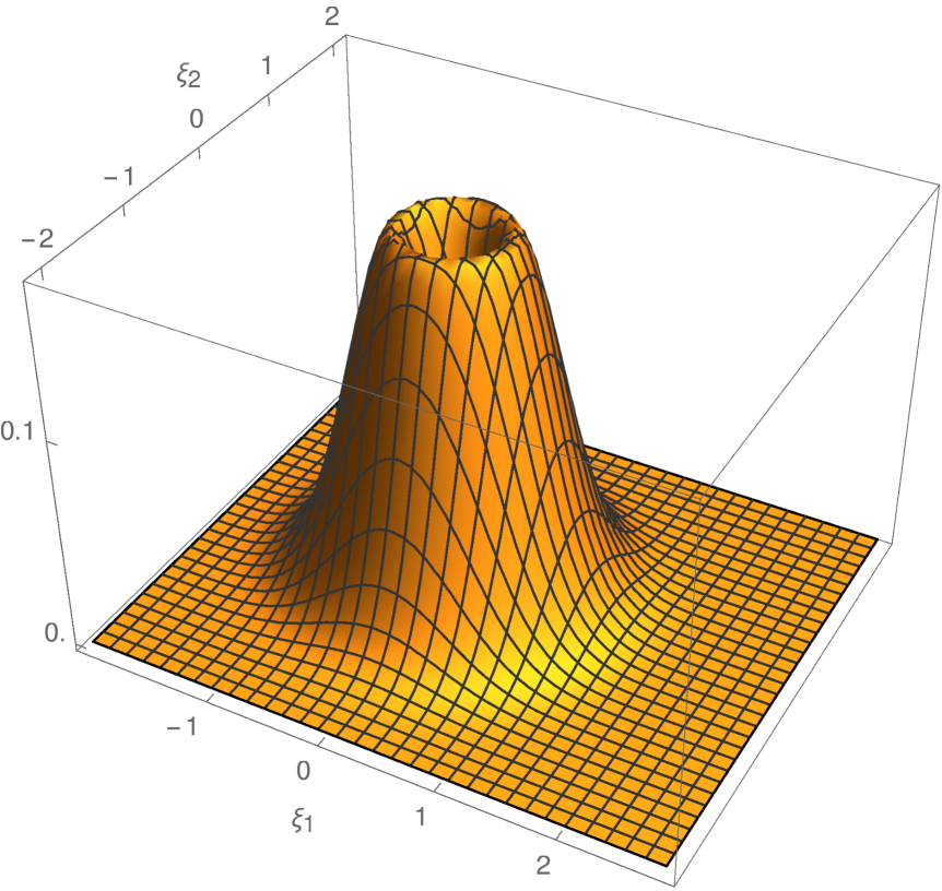
Figure 1: The probability density $|\psi_{1}|^{2}$, with $\psi_{1}$ being a normalized eigenfunction corresponding to the unperturbed eigenvalue $E_{1}:=(\alpha+1/2)\hbar\omega_{c}$, for the values of parameters $\omega_{c}=4$, $\alpha=0.4$. Here $\boldsymbol{\xi}:=\sqrt{\mu\omega_{c}/\hbar}\,\boldsymbol{x}$ is dimensionless.

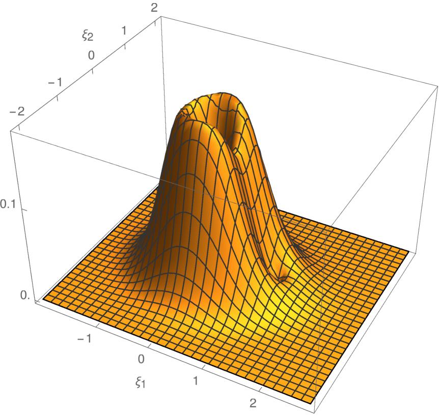
Figure 2: The probability density $|\psi_{2}|^{2}$, with $\psi_{2}$ being a normalized eigenfunction corresponding to the perturbed eigenvalue $E_{2}$ located near $E_{1}$, for the values of parameters $\omega_{c}=4$, $D:=\mu R^{2}\omega_{c}/\hbar=3.5$, $\alpha=0.4$, $\beta=0.7$. Again, $\boldsymbol{\xi}:=\sqrt{\mu\omega_{c}/\hbar}\,\boldsymbol{x}$.

The probability densities of the bound state in the model with one or two solenoids, as mentioned above, are depicted on Figures 1 and 2, respectively. The former case is explicitly solvable while in the latter case we use an approximate formula for the eigenfunction in question which will be derived in Section 4.

2 A single AB solenoid embedded in a uniform magnetic field

2.1 A uniform magnetic field on the universal covering space

As a warm-up, we first study the model with one AB solenoid on the background of a uniform magnetic field. This exercise should provide us with some experience and clues how to proceed in the case of two solenoids. The configuration manifold $M$ is the plane pierced at one point, say the origin, $M=\mathbb{R}^{2}\setminus\{\boldsymbol{0}\}\equiv(0,+\infty)\times S^{1}$ ($S^{1}$ stands for the unit circle). For a electromagnetic vector potential corresponding to a single AB solenoid we can choose

$$\boldsymbol{A}_{AB}=-\frac{\hbar c\alpha}{e}\,\nabla\theta$$

where $\alpha$ is a parameter proportional to the strength of the magnetic flux, see (1.1), and $(r,\theta)$ are polar coordinates. Since the corresponding magnetic Schrödinger operators for $\alpha$ and $\alpha+1$ are unitarily equivalent we shall suppose here and everywhere in what follows that $\alpha\in(0,1)$. A uniform magnetic field can be described by the vector potential (in symmetric gauge)

$$\boldsymbol{A}_{B}=\frac{B}{2}\,\left(\!\begin{array}[]{c}-x_{2}\\ x_{1}\end{array}\!\right).$$ (2.1)

The resulting magnetic Schrödinger operator in polar coordinates reads

$$H_{(B,\alpha)}=-\frac{\hbar^{2}}{2\mu}\!\left(\frac{\partial^{2}}{\partial r^{2}}+\frac{1}{r}\,\frac{\partial}{\partial r}+\frac{1}{r^{2}}\!\left(\frac{\partial}{\partial\theta}-i\,\frac{eBr^{2}}{2\hbar c}+i\alpha\right)^{\!2}\right)\!.$$ (2.2)

The universal covering space of $M$ is $\tilde{M}=(0,+\infty)\times\mathbb{R}$. Then $M=\tilde{M}/2\pi\mathbb{Z}$ (the structure group $\Gamma=2\pi\mathbb{Z}$ acts in the second factor of the Cartesian product). As the first step, we consider a uniform magnetic field on $\tilde{M}$ only. An AB magnetic flux will be incorporated into the model in the following step, in Subsection 2.2, after application of the Schulman-Sunada formula. This means that at this stage we are dealing with the Hamiltonian

$$\tilde{H}_{B}=-\frac{\hbar^{2}}{2\mu}\left(\frac{\partial^{2}}{\partial r^{2}}+\frac{1}{r}\,\frac{\partial}{\partial r}+\frac{1}{r^{2}}\!\left(\frac{\partial}{\partial\theta}-i\,\frac{eBr^{2}}{2\hbar c}\right)^{\!2}\right)$$

which is supposed to act on $L^{2}(\tilde{M},r\mbox{d}r\mbox{d}\theta)$. For a complete set of normalized generalized eigenfunctions of $\tilde{H}_{B}$ one can take $\{f_{n}(p;r,\theta);\ n\in\mathbb{Z}_{+},p\in\mathbb{R}\}$,

$$f_{n}(p;r,\theta)=C_{n}(p)\,r^{|p|}\,L_{n}^{|p|}\!\left(\frac{\mu\omega_{c}r^{2}}{2\hbar}\right)\exp\!\left(-\frac{\mu\omega_{c}r^{2}}{4\hbar}\right)e^{i\,p\theta},$$ (2.3)

where $L_{n}^{\sigma}$ are Laguerre polynomials and

$$C_{n}(p)=\left(\frac{\mu\omega_{c}}{2\hbar}\right)^{\!(|p|+1)/2}\left(\frac{n!}{\pi\,\Gamma(n+|p|+1)}\right)^{\!1/2}\!.$$

One has $\tilde{H}_{B}f_{n}(p)=\lambda_{n}(p)\,f_{n}(p)$ where

$$\lambda_{n}(p)=\left(\frac{p+|p|+1}{2}+n\right)\!\hbar\omega_{c}.$$ (2.4)

The heat kernel on $\tilde{M}$ equals

$$\tilde{p}_{t}(r,\theta;r_{0},\theta_{0})=\sum_{n\in\mathbb{Z}_{+}}\int_{\mathbb{R}}e^{-\lambda_{n}(p)t/\hbar}\,f_{n}(p;r,\theta)\,\overline{f_{n}(p;r_{0},\theta_{0})}\,\mbox{d}p.$$

To proceed further, let us recall the Poisson kernel formula for Laguerre polynomials [5, Eq. (6.2.25)]: for $a,b,c,\sigma>0$,

$$\sum_{n=0}^{\infty}e^{-cn}\,\frac{n!}{\Gamma(n+c+1)}\,L_{n}^{\sigma}(a)L_{n}^{\sigma}(b)$$

$$=\,\frac{e^{\sigma c/2}}{(ab)^{\sigma/2}(1-e^{-c})}\,\exp\!\left(-\frac{(a+b)\,e^{-c}}{1-e^{-c}}\right)I_{\sigma}\!\left(\frac{2\sqrt{ab}\,e^{-c/2}}{1-e^{-c}}\right)\!.$$ (2.5)

Applying (2.5) one finds that

$$\tilde{p}_{t}(r,\theta;r_{0},\theta_{0}) = \frac{\mu\omega_{c}}{4\pi\hbar\sinh(\omega_{c}t/2)}\,\exp\!\left(-\frac{\mu\omega_{c}\,(r^{2}+r_{0}^{\,2})}{4\hbar}\,\coth\!\left(\frac{\omega_{c}t}{2}\right)\right)$$ (2.6)

$$\times\,\int_{\mathbb{R}}e^{-\left(\omega_{c}t/2+i\,(\theta-\theta_{0})\right)p}\,I_{|p|}\!\left(\frac{\mu\omega_{c}rr_{0}}{2\hbar\sinh(\omega_{c}t/2)}\right)\mbox{d}p.$$

Recall that the heat kernel for a charged particle on the plane in a uniform magnetic field, if expressed in polar coordinates, reads [9, §  6.2.1.5]

$$p_{t}(r,\theta;r_{0},\theta_{0}) = \frac{\mu\omega_{c}}{4\pi\hbar\sinh(\omega_{c}t/2)}$$

$$\times\,\exp\!\left(-\frac{\mu\omega_{c}\,(r^{2}+r_{0}^{\,2})}{4\hbar}\,\coth\!\left(\frac{\omega_{c}t}{2}\right)+\frac{\mu\omega_{c}rr_{0}\cosh(\omega_{c}t/2-i(\theta-\theta_{0}))}{2\hbar\sinh(\omega_{c}t/2)}\right)\!.$$

This is the first opportunity in the present paper to demonstrate how the Schulman-Sunada formula works. It claims that the heat kernels $p_{t}$ and $\tilde{p}_{t}$ on $M$ and $\tilde{M}$, respectively, are related by the equation

$$p_{t}(r,\theta;r_{0},\theta_{0})=\sum_{n\in\mathbb{Z}}\tilde{p}_{t}(r,\theta+2\pi n;r_{0},\theta_{0}).$$ (2.8)

This is apparent, indeed, from the Poisson summation rule

$$\sum_{n\in\mathbb{\mathbb{Z}}}\int_{\mathbb{R}}e^{2\pi inp}\,\varphi(p)\,\mbox{d}p=\sum_{n\in\mathbb{Z}}\varphi(n).$$

In fact, (2.8) is then guaranteed by the identity [1, Eq. 9.6.19]

$$\sum_{n\in\mathbb{Z}}e^{zn}\,I_{|n|}(x)=e^{x\cosh(z)},$$

which is valid for $x>0$ and $z\in\mathbb{C}$.

Since $\tilde{M}$ looks locally like $M$ one may regard $p_{t}(r,\theta;r_{0},\theta_{0})$ as a $\Gamma$-invariant function on $\tilde{M}\times\tilde{M}$ which is well defined provided $|\theta-\theta_{0}|<\pi$. Let us complete $\tilde{M}$ with a point $A$ for which $r=0$ and $\theta$ is not determined. The projection $\pi:\tilde{M}\to M$ extends so that $A$ projects onto the excluded point in $\mathbb{R}^{2}$ (the origin). One has

$$p_{t}(A;r,\theta)=p_{t}(r,\theta;A)=\frac{\mu\omega_{c}}{4\pi\hbar\sinh(\omega_{c}t/2)}\,\exp\!\left(-\frac{\mu\omega_{c}\,r^{2}}{4\hbar}\,\coth\!\left(\frac{\omega_{c}t}{2}\right)\!\right)\!.$$ (2.9)

Being inspired by the approach applied in [22] we wish to express the heat kernel on $\tilde{M}$ in the form

$$\tilde{p}_{t}(r,\theta;r_{0},\theta_{0}) = \vartheta(\pi-|\theta-\theta_{0}|)\,p_{t}(r,\theta;r_{0},\theta_{0})$$

$$+\,\int_{0}^{t}p_{s}(r,\theta;A)V(r,\theta,s;r_{0},\theta_{0},t-s)\,p_{t-s}(A;r_{0},\theta_{0})\,\mbox{d}s.$$

Here $\vartheta$ stands for the Heaviside step function ($\vartheta(x)$ equals $1$ for $x>0$ and $0$ otherwise). Concerning the angles, the expression $V(r,\theta,s;r_{0},\theta_{0},t-s)$ should depend only on their difference $\theta-\theta_{0}$. To obtain the sought expression one can use the formula ($x>0$) [1, Eq. 9.6.20]

$$I_{\nu}(x)=\frac{1}{\pi}\,\int_{0}^{\pi}e^{x\cos(\phi)}\,\cos(\nu\phi)\,\mbox{d}\phi-\frac{\sin(\nu\pi)}{\pi}\,\int_{0}^{\infty}e^{-x\cosh(s)-\nu s}\,\mbox{d}s.$$

We find that, for any $z\in\mathbb{C}$,

$$\int_{-\infty}^{\infty}e^{zp}\,I_{|p|}(x)\,\mbox{d}p = e^{x\cosh(z)}\,\vartheta(\pi-|\mathop{\mathrm{missing}}{Im}\nolimits z|)$$

$$+\,\frac{1}{2\pi i}\int_{-\infty}^{\infty}e^{-x\cosh(u)}\left(\frac{1}{z+u+i\pi}-\frac{1}{z+u-i\pi}\right)\!\mbox{d}u.$$

The identity (2.1) is to be applied for $z=-\omega_{c}t/2+i\,(\theta-\theta_{0})$, $x=\mu\omega_{c}rr_{0}/(2\hbar\sinh(\omega_{c}t/2))$. In combination with (2.6) we obtain

$$\hskip-20.00003pt\tilde{p}_{t}(r,\theta;r_{0},\theta_{0})\,=\,\vartheta(\pi-|\theta-\theta_{0}|)\,p_{t}(r,\theta;r_{0},\theta_{0})$$

$$\qquad+\,\frac{\mu\omega_{c}}{4\pi\hbar\sinh(\omega_{c}t/2)}\,\exp\!\left(-\frac{\mu\omega_{c}\,(r^{2}+r_{0}^{\,2})}{4\hbar}\,\coth(\omega_{c}t/2)\right)$$ (2.12)

$$\qquad\quad\times\,\frac{1}{2\pi i}\int_{-\infty}^{\infty}\exp\!\left(-\frac{\mu\omega_{c}rr_{0}}{2\hbar\sinh(\omega_{c}t)}\,\cosh(u)\right)$$

$$\qquad\qquad\qquad\qquad\times\left(\frac{1}{u-\omega_{c}t/2+i\,(\theta-\theta_{0}+\pi)}-\frac{1}{u-\omega_{c}t/2+i\,(\theta-\theta_{0}-\pi)}\right)\mbox{d}u.$$

To bring the formula to the desired structure we seek a substitution $u=u(s)$ such that

$$\frac{\mu\omega_{c}\,(r^{2}+r_{0}^{\,2})}{4\hbar}\,\coth\!\left(\frac{\omega_{c}t}{2}\right)+\frac{\mu\omega_{c}rr_{0}}{2\hbar\sinh(Bt)}\,\cosh(u)$$

$$=\,\frac{\mu\omega_{c}r^{2}}{4\hbar}\,\coth\!\left(\frac{\omega_{c}s}{2}\right)+\frac{\mu\omega_{c}r_{0}^{\,2}}{4\hbar}\,\coth\!\left(\frac{\omega_{c}(t-s)}{2}\right).$$

Simple manipulations lead to the solution

$$u(s)=\ln\!\left(\frac{r\sinh\!\big{(}\omega_{c}(t-s)/2\big{)}}{r_{0}\sinh(\omega_{c}s/2)}\right)\!.$$

Then the second term on the RHS of (2.12) equals

$$\hskip-20.00003pt\frac{\mu}{i\hbar}\left(\frac{\omega_{c}}{4\pi}\right)^{\!2}\int_{0}^{t}\frac{\exp\!\left(-\mu\omega_{c}r^{2}\coth(\omega_{c}s/2)/(4\hbar)\right)}{\sinh(\omega_{c}s/2)}\,\frac{\exp\!\left(-\mu\omega_{c}r_{0}^{\,2}\coth\big{(}\omega_{c}\,(t-s)/2\big{)}/(4\hbar)\right)}{\sinh\big{(}\omega_{c}\,(t-s)/2\big{)}}$$

$$\qquad\qquad\times\!\left(\frac{1}{u(s)-\omega_{c}t/2+i\,(\theta-\theta_{0}+\pi)}-\frac{1}{u(s)-\omega_{c}t/2+i\,(\theta-\theta_{0}-\pi)}\right)\!\mbox{d}s.$$

We conclude that (2.1) holds, indeed, provided we set

$$\hskip-10.00002ptV(r,\theta,s;r_{0},\theta_{0},s_{0}) = \frac{\hbar}{i\mu}\,\Bigg{(}\!\left(U(r,s;r_{0},s_{0})-\frac{\omega_{c}\,(s+s_{0})}{2}+i\,(\theta-\theta_{0}+\pi)\right)^{\!-1}$$

$$\qquad-\left(U(r,s;r_{0},s_{0})-\frac{\omega_{c}\,(s+s_{0})}{2}+i\,(\theta-\theta_{0}-\pi)\right)^{\!-1}\Bigg{)}$$

where

$$U(r,s;r_{0},s_{0})=\ln\!\left(\frac{r\sinh(\omega_{c}s_{0}/2)}{r_{0}\sinh(\omega_{c}s/2)}\right)\!.$$ (2.14)

2.2 An application of the Schulman-Sunada formula

If an AB flux is switched on the Schulman-Sunada formula (2.8) should be modified. In that case it claims that the heat kernel of the magnetic Schrödinger operator corresponding to one AB solenoid in a uniform magnetic field on the plane equals

$$p_{t}^{(\alpha)}(r,\theta;r_{0},\theta_{0})=\sum_{n\in\mathbb{Z}}e^{2\pi i\alpha n}\,\tilde{p}_{t}(r,\theta-2\pi n;r_{0},\theta_{0}).$$ (2.15)

$p_{t}^{(\alpha)}(r,\theta;r_{0},\theta_{0})$ can be interpreted as an equivariant function on $\tilde{M}$ or, alternatively, as a multivalued function on $M$. To obtain an unambiguous expression one has to choose a cut on $M$. We restrict ourselves to values $\theta\in(-\pi,\pi)$, $\theta_{0}=0$. Note that, under these restrictions, $\vartheta(\pi-|\theta-2\pi n-\theta_{0}|)\neq 0$ if and only if $n=0$. We shall need the readily verifiable identity

$$\sum_{n=-\infty}^{\infty}\frac{e^{2\pi i\alpha n}}{w-2\pi n}=\frac{i\,e^{i\alpha w}}{e^{iw}-1}$$ (2.16)

which holds for $\alpha\in(0,1)$ and $w\in\mathbb{C}\setminus 2\pi\mathbb{Z}$. Plugging (2.12) into (2.15) and using (2.16) we obtain

$$\hskip-15.00002ptp_{t}^{(\alpha)}(r,\theta;r_{0},0)=\frac{\mu\omega_{c}}{4\pi\hbar\sinh(\omega_{c}t/2)}$$

$$\qquad\qquad\qquad\qquad\times\exp\!\left(-\frac{\mu\omega_{c}\,(r^{2}+r_{0}^{\,2})}{4\hbar}\,\coth\!\left(\frac{\omega_{c}t}{2}\right)\!+\frac{\mu\omega_{c}rr_{0}\cosh(\omega_{c}t/2-i\theta)}{2\hbar\sinh(\omega_{c}t/2)}\right)$$

$$\qquad\qquad\qquad-\,\frac{\sin(\pi\alpha)\,\mu\omega_{c}}{4\pi^{2}\hbar\sinh(\omega_{c}t/2)}\,\exp\!\left(-\frac{\mu\omega_{c}\,(r^{2}+r_{0}^{\,2})}{4\hbar}\,\coth(\omega_{c}t/2)\right)$$ (2.17)

$$\qquad\qquad\qquad\qquad\times\int_{\mathbb{R}}\exp\!\left(-\frac{\mu\omega_{c}rr_{0}\cosh(u+\omega_{c}t/2)}{2\hbar\sinh(\omega_{c}t/2)}\right)\!\frac{e^{\alpha(u+i\theta)}}{1+e^{u+i\theta}}\,\mbox{d}u.$$

A common approach how to derive a formula for $p_{t}^{(\alpha)}(r,\theta;r_{0},0)$ is based on the eigenfunction expansion. Referring to (2.3), (2.4), the functions

$$f_{n,m}(r,\theta):=f_{n}(m+\alpha;r,\theta),\ \ \text{with}\ n\in\mathbb{Z}_{+},m\in\mathbb{Z},$$ (2.18)

form an orthonormal basis in $L^{2}(M,r\mbox{d}r\mbox{d}\theta)$. At the same time, the functions

$$f^{\prime}_{n,m}(r,\theta)=e^{-i\alpha\theta}f{}_{n,m}(r,\theta)$$

are eigenfunctions of $H_{(B,\alpha)}$ (see (2.2)), $H_{(B,\alpha)}f^{\prime}_{n,m}=\lambda_{n,m}f^{\prime}_{n,m}$ where

$$\lambda_{n,m}:=\lambda_{n}(m+\alpha)=\!\left(\frac{m+\alpha+|m+\alpha|+1}{2}+n\right)\!\hbar\omega_{c}.$$ (2.19)

Then

$$p_{t}^{(\alpha)}(r,\theta;r_{0},0)=\sum_{n\in\mathbb{Z}_{+}}\sum_{m\in\mathbb{Z}}\,e^{-t\lambda_{n,m}/\hbar}f_{n,m}(r,\theta)\,\overline{f_{n,m}(r_{0},0)}\,.$$ (2.20)

Conversely, (2.20) suggests that $p_{t}^{(\alpha)}$ contains all information about the spectral properties of $H_{(B,\alpha)}$ which can be extracted, in principle, with the aid of asymptotic analysis of the heat kernel as $t\to+\infty$. As an example, let us check just the first two leading asymptotic terms of (2.17). Referring to (B.2), it is straightforward to derive the asymptotic expansion

$$\hskip-20.00003ptp_{t}^{(\alpha)}(r,\theta;r_{0},0)\,=\Bigg{(}\frac{\mu\omega_{c}}{2\pi\hbar}\,\exp\!\left(-\frac{\mu\omega_{c}\,(r^{2}+r_{0}^{\,2})}{4\hbar}+\frac{\mu\omega_{c}rr_{0}}{2\hbar}\,e^{-i\theta}\right)$$

$$-\,\frac{\sin(\pi\alpha)\mu\omega_{c}}{2\pi^{2}\hbar}\,\exp\!\left(-\frac{\mu\omega_{c}\,(r^{2}+r_{0}^{\,2})}{4\hbar}\right)\int_{\mathbb{R}}\exp\!\left(-\frac{\mu\omega_{c}rr_{0}}{2\hbar}\,e^{u}\right)\frac{e^{\alpha(u+i\theta)}}{1+e^{u+i\theta}}\,\mbox{d}u\Bigg{)}e^{-\omega_{c}t/2}$$

$$+\,\frac{\mu\omega_{c}}{2\pi\Gamma(1+\alpha)\hbar}\,\exp\!\left(-\frac{\mu\omega_{c}\,(r^{2}+r_{0}^{\,2})}{4\hbar}\right)\left(\frac{\mu\omega_{c}rr_{0}}{2\hbar}\right)^{\!\alpha}e^{i\alpha\theta}\,e^{-(\alpha+1/2)\omega_{c}t}+O(e^{-3\omega_{c}t/2}).$$

(2.21)

Comparing (2.20) with (2.21), the asymptotic expansion covers the terms in the former formula with $n=0$ and $m\in-\mathbb{Z}_{+}$. For $n=0$ and $m=0$ one reveals the expression for the eigenfunction $f_{0,0}(r,\theta)$ corresponding to the simple eigenvalue $\lambda_{0,0}=(\alpha+1/2)\hbar\omega_{c}$, see (2.18), (2.19).

For $n=0$ and $m<0$, $\lambda_{0,m}=\hbar\omega_{c}/2$ is the infinitely degenerate lowest Landau level. Hence the expression standing at $e^{-\omega_{c}t/2}$ on the RHS of (2.21) should be the kernel of the orthogonal projection onto the corresponding eigenspace. This is to say that

$$\hskip-20.00003pt\sum_{m\in\mathbb{Z},\,m<0}f_{0,m}(r,\theta)\,\overline{f_{0.m}(r_{0},0)}\,=\,\frac{\mu\omega_{c}}{2\pi\hbar}\,\exp\!\left(-\frac{\mu\omega_{c}\,(r^{2}+r_{0}^{\,2})}{4\hbar}+\frac{\mu\omega_{c}rr_{0}}{2\hbar}\,e^{-i\theta}\right)$$

$$\qquad\qquad-\,\frac{\sin(\pi\alpha)\mu\omega_{c}}{2\pi^{2}\hbar}\,\exp\!\left(-\frac{\mu\omega_{c}\,(r^{2}+r_{0}^{\,2})}{4\hbar}\right)\int_{\mathbb{R}}\exp\!\left(-\frac{\mu\omega_{c}rr_{0}}{2\hbar}\,e^{u}\right)\frac{e^{\alpha(u+i\theta)}}{1+e^{u+i\theta}}\,\mbox{d}u.$$

(2.22)

Observing that $L_{0}^{\sigma}(x)=1$, (2.22) amounts to

$$\exp(\rho e^{i\phi})\,e^{i\alpha\phi}-\frac{\sin(\pi\alpha)}{\pi}\int_{\mathbb{R}}\exp(-\rho e^{u})\frac{e^{\alpha u}}{1+e^{u-i\phi}}\,\mbox{d}u=\sum_{m=1}^{\infty}\frac{\rho^{m-\alpha}}{\Gamma(m+1-\alpha)}\,e^{im\phi}$$ (2.23)

for $\rho>0$ and $\phi\in(-\pi,\pi)$ (and $\alpha\in(0,1)$). But (2.23) follows from (A.7).

3 The two-solenoid case

3.1 The heat kernel on the universal covering space

The configuration space for the Aharonov-Bohm effect with two vortices is the plane with two excluded points, $M=\mathbb{R}^{2}\setminus\{\boldsymbol{a},\boldsymbol{b}\}$. $M$ is a flat Riemannian manifold and the same is true for the universal covering space $\tilde{M}$. By the very construction, $\tilde{M}$ is connected and simply connected, and one can identify $M=\tilde{M}/\Gamma$ where $\Gamma$ is the fundamental group of $M$. Let $\pi:\tilde{M}\to M$ be the projection.

The fundamental group $\Gamma$ in this case is known to be the free group with two generators. For the first generator, called $g_{a}$, one can choose the homotopy class of a simple positively oriented loop winding once around the point $\boldsymbol{a}$ and leaving the point $\boldsymbol{b}$ in the exterior. Analogously one can choose the second generator, $g_{b}$, by interchanging the role of $\boldsymbol{a}$ and $\boldsymbol{b}$.

It is convenient to complete the manifold $\tilde{M}$ by a countable set of points $\mathcal{A}\cup\mathcal{B}$ lying on the border of $\tilde{M}$ and projecting onto the excluded points, $\pi(\mathcal{A})=\{\boldsymbol{a}\}$ and $\pi(\mathcal{B})=\{\boldsymbol{b}\}$.

The geometry of $\tilde{M}$ is locally the same as that of the plane but globally it exhibits some substantially distinct features. In particular, not always a couple of points from $\tilde{M}$ can be connected by a segment (a geodesic curve). For $\boldsymbol{x},\boldsymbol{y}\in\tilde{M}\cup\mathcal{A}\cup\mathcal{B}$ set $\chi(\boldsymbol{x},\boldsymbol{y})=1$ if the points $\boldsymbol{x}$, $\boldsymbol{y}$ can be connected by a segment, and $\chi(\boldsymbol{x},\boldsymbol{y})=0$ otherwise.

Our first goal is to construct the heat kernel on $\tilde{M}$ for a charged particle subjected to a uniform magnetic field. A starting point is again formula (2.1) for the heat kernel on the plane which can be rewritten in Cartesian coordinates as

$$p_{t}(\boldsymbol{x},\boldsymbol{x}_{0})=\frac{\mu\omega_{c}}{4\pi\hbar\sinh(Bt)}\,\exp\!\left(-\frac{\mu\omega_{c}\,|\boldsymbol{x}-\boldsymbol{x}_{0}|^{2}}{4\hbar}\,\coth\!\left(\frac{\omega_{c}t}{2}\right)+i\,\frac{\mu\omega_{c}}{2\hbar}\,\boldsymbol{x}\wedge\boldsymbol{x}_{0}\right)\!.$$ (3.1)

Here we have used the notation $\boldsymbol{x}\wedge\boldsymbol{y}:=x_{1}y_{2}-x_{2}y_{1}$. Note that $\boldsymbol{x}\wedge\boldsymbol{x}_{0}=-rr_{0}\sin(\theta-\theta_{0})$.

Our choice of the gauge for the electromagnetic vector potential depends on the choice of the origin of coordinates. Moving the origin of coordinates from $\boldsymbol{0}$ to a point $\boldsymbol{y}$ one has the transformation rule

$$p_{t}^{\text{transformed}}(\boldsymbol{x};\boldsymbol{x}_{0})=e^{i\mu\omega_{c}/(2\hbar)\,\boldsymbol{y}\wedge\boldsymbol{x}}\,p_{t}(\boldsymbol{x};\boldsymbol{x}_{0})\,e^{-i\mu\omega_{c}/(2\hbar)\,\boldsymbol{y}\wedge\boldsymbol{x}_{0}}.$$ (3.2)

For the corresponding Hamiltonian, now written in Cartesian coordinates as

$$H_{B}=-\frac{\hbar^{2}}{2\mu}\left(\frac{\partial}{\partial x_{1}}+\frac{ieB}{2\hbar c}\,x_{2}\right)^{\!2}-\left(\frac{\partial}{\partial x_{2}}-\frac{ieB}{2\hbar c}\,x_{1}\right)^{\!2},$$ (3.3)

this means the unitary transformation

$$H_{B}^{\text{transformed}}=e^{-i\,eB/(2\hbar c)\,(y_{1}x_{2}-y_{2}x_{1})}H_{B}\,e^{i\,eB/(2\hbar c)\,(y_{1}x_{2}-y_{2}x_{1})}.$$

Shifting our focus to the covering space, suppose $\boldsymbol{x}_{0},\boldsymbol{x}\in\tilde{M}\cup\mathcal{A}\cup\mathcal{B}$ and $C\in\mathcal{A}\cup\mathcal{B}$ fulfill $\chi(\boldsymbol{x}_{0},C)=\chi(\boldsymbol{x},C)=1$, i.e. $\boldsymbol{x}_{0}$ and $\boldsymbol{x}$ can be both connected with $C$ by a segment. In addition, suppose we are given $t_{0},t_{1}>0$. In accordance with (LABEL:eq:V_1sol), (2.14), we put

$$\hskip-20.00003ptV\!\left(\!\!\begin{array}[]{c}\boldsymbol{x},C,\boldsymbol{x}_{0}\\ t_{1},t_{0}\end{array}\!\!\right)$$

$$=\,\frac{\hbar}{i\mu}\left(\!\left(U-\frac{\omega_{c}\,(t_{1}+t_{0})}{2}+i\,(\Theta+\pi)\right)^{\!-1}-\left(U-\frac{\omega_{c}\,(t_{1}+t_{0})}{2}+i\,(\Theta-\pi)\right)^{\!-1}\right)$$

where

$$U=\ln\!\left(\frac{\mathop{\mathrm{missing}}{dist}\nolimits(\boldsymbol{x},C)\,\sinh(\omega_{c}t_{0}/2)}{\mathop{\mathrm{missing}}{dist}\nolimits(\boldsymbol{x}_{0},C)\,\sinh(\omega_{c}t_{1}/2)}\right)$$

and $\Theta=\angle\,\boldsymbol{x}_{0},C,\boldsymbol{x}\in\mathbb{R}$ is the oriented angle.

Denote by $\tilde{\mathscr{C}}(\boldsymbol{x},\boldsymbol{x}_{0})$ the set of all piecewise geodesic curves

$$\gamma:\boldsymbol{x}_{0}\to C_{1}\to\ldots\to C_{n}\to\boldsymbol{x}$$

with the inner vortices $C_{j}$, $1\leq j\leq n$, belonging to the set of extreme points $\mathcal{A}\cup\mathcal{B}$. This means that the equations $\chi(\boldsymbol{x}_{0},C_{1})=\chi(C_{1},C_{2})=\ldots=\chi(C_{n},\boldsymbol{x})=1$ hold. Let us denote by $|\gamma|=n\in\mathbb{N}$ the length of a sequence $(C_{1},C_{2},\ldots,C_{n})$. To simplify the notation we set everywhere where convenient $C_{0}=\boldsymbol{x}_{0}$ and $C_{n+1}=\boldsymbol{x}$. Then formula (2.1) for the heat kernel $\tilde{p}_{t}(\boldsymbol{x},\boldsymbol{x}_{0})$ on the universal covering space $\tilde{M}$ generalizes to the model with two AB fluxes as follows

$$\tilde{p}_{t}(\boldsymbol{x},\boldsymbol{x}_{0}) = \chi(\boldsymbol{x},\boldsymbol{x}_{0})\,p_{t}(\boldsymbol{x},\boldsymbol{x}_{0})$$ (3.12)

$$+\,\sum_{\gamma\in\,\tilde{\mathscr{C}}(x,x_{0})}\,\int_{0}^{\infty}\mathrm{d}t_{n}\int_{0}^{\infty}\mathrm{d}t_{n-1}\,\cdots\,\mathrm{\int_{0}^{\infty}d}t_{0}\,\delta(t_{n}+t_{n-1}+\ldots+t_{0}-t)$$

$$\qquad\times\,p_{t_{n}}(\boldsymbol{x},C_{n})\,p_{t_{n-1}}(C_{n},C_{n-1})\,\cdots\,p_{t_{0}}(C_{1},\boldsymbol{x}_{0})$$

$$\qquad\times\,V\!\left(\!\begin{array}[]{c}\boldsymbol{x},C_{n},C_{n-1}\\ t_{n},t_{n-1}\end{array}\!\right)V\!\left(\!\begin{array}[]{c}C_{n},C_{n-1},C_{n-2}\\ t_{n-1},t_{n-2}\end{array}\!\right)\cdots\,V\!\left(\!\begin{array}[]{c}C_{2},C_{1},\boldsymbol{x}_{0}\\ t_{1},t_{0}\end{array}\!\right)\!.$$

Here again, the symbol $p_{t}(\boldsymbol{x},\boldsymbol{y})$ is understood as the lift of the heat kernel (3.1) from the plane to $\tilde{M}$ provided $\boldsymbol{x}$ and $\boldsymbol{y}$ can be connected by a segment.

A detailed verification of (3.12) in the particular case when the background uniform magnetic field is absent can be found in [15]. The general case comprising a uniform magnetic field as well can be treated in the very same manner. We omit the details here since this would be exceedingly lengthy.

3.2 An application of the Schulman-Sunada formula

One-dimensional unitary representations $\Lambda$ of $\Gamma$ are determined by two numbers $\alpha$, $\beta$, $0\leq\alpha,\beta<1$, such that

$$\Lambda(g_{a})=e^{2\pi i\alpha},\textrm{\leavevmode\nobreak\ }\Lambda(g_{b})=e^{2\pi i\beta}.$$

Fix $\alpha,\beta\in(0,1)$ and, correspondingly, a representation $\Lambda$. The values $\alpha$ and $\beta$ are proportional to the strengths of the AB magnetic fluxes through the vortices $\boldsymbol{a}$ and $\boldsymbol{b}$, respectively (see (1.1)). The heat kernel $p_{t}^{\Lambda}(\boldsymbol{x},\boldsymbol{x}_{0})$ for a charged particle on the plane pierced by these two AB fluxes and subjected to a uniform magnetic field can again be derived with the aid the Schulman-Sunada formula, now written in the form

$$p_{t}^{\Lambda}(\boldsymbol{x},\boldsymbol{x}_{0})=\sum_{g\in\Gamma}\Lambda(g^{-1})\,\tilde{p}_{t}(g\cdot\boldsymbol{x},\boldsymbol{x}_{0}).$$ (3.13)

Concerning the corresponding magnetic Schrödinger operator $H_{\Lambda}$, it is convenient to pass to a unitarily equivalent formulation. Suppose the vortices $\boldsymbol{a}$, $\boldsymbol{b}$ lie on the first axis and $\boldsymbol{a}$ is located left to $\boldsymbol{b}$. Let us cut the plane along two half-lines,

$$L_{a}:=(-\infty,a_{1})\times\{0\}\textrm{\leavevmode\nobreak\ and\leavevmode\nobreak\ }L_{b}:=(b_{1},+\infty)\times\{0\}.$$

Let $(r_{c},\theta_{c})$ be polar coordinates centered at a point $\boldsymbol{c}$, $\boldsymbol{c}=\boldsymbol{a},\boldsymbol{b}$. Furthermore, the values $\theta_{a}=\pm\pi$ correspond to the two sides of the cut $L_{a}$, and similarly for $\theta_{b}$ and $L_{b}$. The geometrical arrangement is depicted on Figure 3.

The electromagnetic vector potential in the discussed model is the sum of the vector potential $\boldsymbol{A}_{B}$ given in (2.1) and the AB vector potential

$$\boldsymbol{A}_{AB}=-\frac{\hbar c}{e}\,(\alpha\nabla\theta_{a}+\beta\nabla\theta_{b}).$$

The region $\mathcal{D}=\mathbb{R}^{2}\setminus(L_{a}\cup L_{b})$ is simply connected and therefore one can eliminate the vector potential $\boldsymbol{A}_{AB}$ by means of a gauge transform. This way one can pass to a unitarily equivalent Hamiltonian $H_{\Lambda}^{\prime}\simeq H_{\Lambda}$ acting as the differential operator $H_{B}$ in $L^{2}(\mathbb{R}^{2},\mbox{d}^{2}x)$, see (3.3), and whose domain is determined by the boundary conditions along the cut,

$$\psi(r_{a},\theta_{a}=\pi)=e^{2\pi\,i\,\alpha}\psi(r_{a},\theta_{a}=-\pi),\textrm{\leavevmode\nobreak\ }\partial_{\theta_{a}}\psi(r_{a},\theta_{a}=\pi)=e^{2\pi\,i\,\alpha}\,\partial_{\theta_{a}}\psi(r_{a},\theta_{a}=-\pi)\,,$$

(3.14)

$$\psi(r_{b},\theta_{b}=\pi)=e^{2\pi\,i\,\beta}\psi(r_{b},\theta_{b}=-\pi),\textrm{\leavevmode\nobreak\ }\ \partial_{\theta_{b}}\psi(r_{b},\theta_{b}=\pi)=e^{2\pi\,i\,\beta}\,\partial_{\theta_{b}}\psi(r_{b},\theta_{b}=-\pi)\,.$$

In addition, one should impose the regular boundary condition at the vortices, namely $\psi(\boldsymbol{a})=\psi(\boldsymbol{b})=0$.

One can embed $\mathcal{D}\subset\tilde{M}$ as a fundamental domain of $\Gamma$. The heat kernel ${p^{\prime}_{t}}^{\Lambda}(\boldsymbol{x},\boldsymbol{x}_{0})$ associated with ${H^{\prime}}_{\Lambda}$ can be simply obtained as the restriction to $\mathcal{D}$ of the heat kernel $p_{t}^{\Lambda}(\boldsymbol{x},\boldsymbol{x}_{0})$ associated with $H_{\Lambda}$ provided $p_{t}^{\Lambda}(\boldsymbol{x},\boldsymbol{x}_{0})$ is regarded as a $\Lambda$-equivariant function on $\tilde{M}\times\tilde{M}$. In order to simplify the discussion of phases we shall assume that either $\boldsymbol{x}$, $\boldsymbol{x}_{0}$ belong both to the upper half plane or $\boldsymbol{x}_{0}$ lies on the segment connecting $\boldsymbol{a}$ and $\boldsymbol{b}$. In that case the segment $\overline{\boldsymbol{x}_{0}\boldsymbol{x}}$ intersects none of the cuts $L_{a}$ and $L_{b}$.

Fix $t>0$. Let $\mathscr{C}$ be the set of all finite alternating sequence of points $\boldsymbol{a}$ and $\boldsymbol{b}$, i.e. $\overline{\gamma}\in\mathscr{C}$ if $\overline{\gamma}=(\boldsymbol{c}_{1},\ldots,\boldsymbol{c}_{n})$ for some $n\in\mathbb{N}$ and $\boldsymbol{c}_{j}\in\{\boldsymbol{a},\boldsymbol{b}\}$, $\boldsymbol{c}_{j}\neq\boldsymbol{c}_{j+1}$. Relate to $\overline{\gamma}$ a piecewise geodesic path in $M$, namely

$$\boldsymbol{x}_{0}\to\boldsymbol{c}_{1}\to\ldots\to\boldsymbol{c}_{n}\to\boldsymbol{x}.$$ (3.15)

Let us consider all possible piecewise geodesic paths in $\tilde{M}$,

$$\gamma:\boldsymbol{x}_{0}\to C_{1}\to\ldots\to C_{n}\to g\cdot\boldsymbol{x},$$ (3.16)

with $C_{j}\in\mathcal{A}\cup\mathcal{B}$ and $g\in\Gamma$, covering the path (3.15). Then $C_{j}\in\mathcal{A}$ if and only if $\boldsymbol{c}_{j}=\boldsymbol{a}$, and $C_{j}\in\mathcal{B}$ if and only if $\boldsymbol{c}_{j}=\boldsymbol{b}$. For $n\geq 2$, denote the oriented angles $\angle\,\boldsymbol{x}_{0},\boldsymbol{c}_{1},\boldsymbol{c}_{2}=\theta_{0}$ and $\angle\,\boldsymbol{c}_{n-1},\boldsymbol{c}_{n},\boldsymbol{x}=\theta$. Then angles at the corresponding vortices in the path $\gamma$ take the values $\angle\,\boldsymbol{x}_{0},C_{1},C_{2}=\theta_{0}+2\pi k_{1}$, $\angle\,C_{n-1},C_{n},g\cdot\boldsymbol{x}=\theta+2\pi k_{n}$ and $\angle\,C_{j},C_{j+1},C_{j+2}=2\pi k_{j+1}$ for $1\leq j\leq n-2$ (if $n\geq 3$), where $k_{1},\ldots,k_{n}$ are integers. For $n=1$, $\angle\,\boldsymbol{x}_{0},C_{1},g\cdot\boldsymbol{x}=\angle\,\boldsymbol{x}_{0},c_{1},\boldsymbol{x}+2\pi k_{1}$, $k_{1}\in\mathbb{Z}$. Let us emphasize that any values $k_{1},\ldots,k_{n}\in\mathbb{Z}$ are possible, and these $n$-tuples of integers are in one-to-one correspondence with the group elements $g$ occurring in (3.16). The representation $\Lambda$ takes on $g$ the value

$$\Lambda(g)=\exp(2\pi i(k_{1}\sigma_{1}+\ldots+k_{n}\sigma_{n}))$$

where $\sigma_{j}\in\{\alpha,\beta\}$ and $\sigma_{j}=\alpha$ if $\boldsymbol{x}_{j}=\boldsymbol{a}$, and $\sigma_{j}=\beta$ if $\boldsymbol{c}_{j}=\boldsymbol{b}$.

Note that (2.16) implies that

$$\sum_{k\in\mathbb{Z}}e^{-2\pi\mathrm{i}\alpha k}\left(\frac{1}{z+i\,(2k+1)\pi}-\frac{1}{z+i\,(2k-1)\pi}\right)=\frac{2}{i}\,\sin(\pi\alpha)\,\frac{e^{\alpha z}}{1+e^{z}}$$ (3.17)

holds for $0<\alpha<1$ and $z\in\mathbb{C}$. Observe also that the expression

$$p_{t_{n}}(\boldsymbol{x},C_{n})\,p_{t_{n-1}}(C_{n},C_{n-1})\,\cdots\,p_{t_{0}}(C_{1},\boldsymbol{x}_{0})$$

in the integrand in (3.12) in fact does not depend on the integers $k_{1},\ldots,k_{n}$, see (2.9). Consequently, using (3.17) one can carry out a partial summation over $k_{1},\ldots,k_{n}$ in (3.13), (3.12). This way the summation over $g\in\Gamma$ in (3.13) reduces to a sum over $\overline{\gamma}\in\mathscr{C}$.

Further we apply the following transformation of coordinates for a given $t>0$ and $\overline{\gamma}\in\mathscr{C}$. Denote again by $R$ the distance between $\boldsymbol{a}$ and $\boldsymbol{b}$. Put $r_{0}=|\boldsymbol{x}_{0}-\boldsymbol{c}_{1}|$, $r_{j}=|\boldsymbol{c}_{j}-\boldsymbol{c}_{j+1}|=R$ for $0<j<n$, and $r_{n}=|\boldsymbol{c}_{n}-\boldsymbol{x}|$. The transformation sends an $(n+1)$-tuple of positive numbers $(t_{0},t_{1},\ldots,t_{n})$ fulfilling

$$t_{0}+t_{1}+\cdots+t_{n}=t$$

to $u\in\mathbb{R}^{n}$,

$$u_{j}=\ln\!\left(\frac{r_{j}\sinh(\omega_{c}t_{j-1}/2)}{r_{j-1}\sinh(\omega_{c}t_{j}/2)}\right)-\frac{\omega_{c}\,(t_{j-1}+t_{j})}{2},\ 1\leq j\leq n.$$

Let us regard $t_{1},t_{2},\ldots,t_{n}>0$, obeying $0<t_{1}+t_{2}+\cdots+t_{n}<t$, as independent variables and let $t_{0}=t-t_{1}-t_{2}-\cdots-t_{n}$. The transformation is invertible, the inverse image of $u\in\mathbb{R}^{n}$ is

$$t_{j}=\frac{1}{\omega_{c}}\ln\!\left(\frac{1+T_{j}(u)+e^{-\omega_{c}t}\left(T_{n}(u)-T_{j}(u)\right)}{1+T_{j-1}(u)+e^{-\omega_{c}t}\left(T_{n}(u)-T_{j-1}(u)\right)}\right),\text{ }\ j=1,2,\ldots,n.$$

where we have put

$$T_{j}(u)=\sum_{k=1}^{j}\frac{r_{k}}{r_{0}}\exp\!\left(-\sum_{\ell=1}^{k}u_{\ell}\right),\text{ }\ j=0,1,\ldots,n;$$

particularly, $T_{0}(u)=0$.

By some routine manipulations one can verify that

$$\mbox{d}u_{1}\mbox{d}u_{2}\ldots\mbox{d}u_{n}=\left(\frac{\omega_{c}}{2}\right)^{\!n}\frac{\sinh(\omega_{c}t/2)}{\sinh(\omega_{c}t_{0}/2)\sinh(\omega_{c}t_{1}/2)\cdots\sinh(\omega_{c}t_{n})}\,\mbox{d}t_{1}\mbox{d}t_{2}\ldots\mbox{d}t_{n}.$$

Furthermore,

$$\sum_{j=0}^{n}r_{j}^{\,2}\coth\!\left(\frac{\omega_{c}t_{j}}{2}\right)\!=\coth\!\left(\frac{\omega_{c}t}{2}\right)\sum_{j=0}^{n}r_{j}^{\,2}+\frac{2}{\sinh(\omega_{c}t/2)}\,\sum_{\begin{subarray}{c}j,k=0\\ j<k\end{subarray}}^{n}r_{j}r_{k}\cosh\!\left(\frac{\omega_{c}t}{2}+\sum_{s=j+1}^{k}u_{s}\!\right)\!.$$

Thus we arrive at the desired formula. Suppose $a_{1},b_{1}\in\mathbb{R\equiv\mathbb{R}}\times\{0\}\subset\mathbb{R}^{2}$, $a_{1}<b_{1}$, $a_{2}=b_{2}=0$, $\alpha,\beta\in(0,1)$ and $\boldsymbol{x}_{0},\boldsymbol{x}\in\mathbb{R}_{+}^{2}$ (the upper half-plane), $t>0$. Put $R=b_{1}-a_{1}$. Then

$${p^{\prime}_{t}}^{\Lambda}(x,x_{0})={p^{\prime}_{t}}^{\Lambda}(I)+{p^{\prime}_{t}}^{\Lambda}(II)+{p^{\prime}_{t}}^{\Lambda}(III)$$ (3.18)

where

$${p^{\prime}_{t}}^{\Lambda}(I)=\frac{\mu\omega_{c}}{4\pi\hbar\sinh(\omega_{c}t/2)}\,\exp\!\left(-\frac{\mu\omega_{c}\,|\boldsymbol{x}-\boldsymbol{x}_{0}|^{2}}{4\hbar}\,\coth\!\left(\frac{\omega_{c}t}{2}\right)+i\,\frac{\mu\omega_{c}}{2\hbar}\,\boldsymbol{x}\wedge\boldsymbol{x}_{0}\right)\!,$$ (3.19)

$$\hskip-50.00008pt{p^{\prime}_{t}}^{\Lambda}(II)\,=\,-\,\frac{\mu\omega_{c}}{4\pi^{2}\hbar\sinh(\omega_{c}t/2)}\,\sum_{\boldsymbol{c}\in\{\boldsymbol{a},\boldsymbol{b}\}}\sin(\pi\sigma)$$

$$\qquad\qquad\times\,\exp\!\left(-\frac{\mu\omega_{c}\,(r^{2}+r_{0}^{\,2})}{4\hbar}\,\coth\!\left(\frac{\omega_{c}t}{2}\right)+i\,\frac{\mu\omega_{c}}{2\hbar}\,(\boldsymbol{x}-\boldsymbol{x}_{0})\wedge\boldsymbol{c}\right)$$ (3.20)

$$\qquad\qquad\times\,\int_{\mathbb{R}}\exp\!\left(-\frac{\mu\omega_{c}\,rr_{0}}{2\hbar\sinh(\omega_{c}t/2)}\,\cosh\!\left(\frac{\omega_{c}t}{2}+u\right)\!\right)\frac{e^{\sigma\,(u+i\theta_{1,0})}}{1+e^{u+i\theta_{1,0}}}\,\mbox{d}u,$$

$$\hskip-20.00003pt{p^{\prime}_{t}}^{\Lambda}(x,x_{0})\,=\,\sum_{\overline{\gamma}\in\mathscr{C},\,n\geq 2}\frac{(-1)^{n}\mu\omega_{c}}{4\pi^{n+1}\hbar\sinh(\omega_{c}t/2)}$$

$$\qquad\times\,\exp\!\left(-\frac{\mu\omega_{c}\,(r^{2}+(n-1)R^{2}+r_{0}^{\,2})}{4\hbar}\,\coth\!\left(\frac{\omega_{c}t}{2}\right)+i\,\frac{\mu\omega_{c}}{2\hbar}\,(\boldsymbol{x}\wedge\boldsymbol{c}_{n}+\boldsymbol{c}_{1}\wedge\boldsymbol{x}_{0})\right)$$

$$\qquad\times\,\int_{\mathbb{R}^{n}}\exp\!\left(-\frac{\mu\omega_{c}}{2\hbar\sinh(\omega_{c}t/2)}\,\sum_{0\leq j<k\leq n}r_{k}r_{j}\cosh\!\left(\frac{\omega_{c}t}{2}+\sum_{s=j+1}^{k}u_{s}\right)\right)$$ (3.21)

$$\qquad\times\,\frac{\sin(\pi\sigma_{n})\,e^{\sigma_{n}\,(u_{n}+i\theta)}}{1+e^{u_{n}+i\theta}}\left(\prod_{j=2}^{n-1}\,\frac{\sin(\pi\sigma_{j})\,e^{\sigma_{j}u_{j}}}{1+e^{u_{j}}}\right)\frac{\sin(\pi\sigma_{1})\,e^{\sigma_{1}\,(u_{1}+i\theta_{0})}}{1+e^{u_{1}+i\theta_{0}}}\,\mbox{d}^{n}u.$$

Here we have put, in (3.20), $r=|\boldsymbol{x}-\boldsymbol{c}|$, $r_{0}=|\boldsymbol{x}_{0}-\boldsymbol{c}|$, $\theta_{1,0}=\angle\,\boldsymbol{x}_{0},\boldsymbol{c},\boldsymbol{x}$ and $\sigma=\alpha$ (respectively, $\beta$) if $\boldsymbol{c}=\boldsymbol{a}$ (respectively, $\boldsymbol{b}$), and in (3.21), $\overline{\gamma}=(\boldsymbol{c}_{1},\boldsymbol{c}_{2},\ldots,\boldsymbol{c}_{n})$, $r=r_{n}=|\boldsymbol{x}-\boldsymbol{c}_{n}|$, $r_{0}=|\boldsymbol{x}_{0}-\boldsymbol{c}_{1}|$, $r_{j}=R$ for $1\leq j\leq n-1$, $\theta=\angle\,\boldsymbol{c}_{n-1},\boldsymbol{c}_{n},\boldsymbol{x}$, $\theta_{0}=\angle\,\boldsymbol{x}_{0},\boldsymbol{c}_{1},\boldsymbol{c}_{2}$ and $\sigma_{j}=\alpha$ (respectively, $\beta$) if $\boldsymbol{c}_{j}=\boldsymbol{a}$ (respectively, $\boldsymbol{b}$).

4 An approximate formula for a $2$-solenoid eigenfunction

4.1 An approximation of the heat kernel

We are still using the notation introduced above, in particular, $(r_{a},\theta_{a})$ denote polar coordinates with respect to the center $\boldsymbol{a}$, with the equations $\theta_{a}=\pm\pi$ defining the two sides of the cut $L_{a}$, and similarly for $(r_{b},\theta_{b})$ and $L_{b}$. Furthermore, $R=\mathop{\mathrm{missing}}{dist}\nolimits(\boldsymbol{a},\boldsymbol{b})$ and $\boldsymbol{a},\boldsymbol{b}\in\mathbb{R}\times\{0\}\subset\mathbb{R}^{2}$. Assume that $\boldsymbol{x}_{0}$ is an inner point of the segment $\overline{\boldsymbol{a}\boldsymbol{b}}$, $\boldsymbol{x}\in\mathbb{R}^{2}\setminus(L_{a}\cup L_{b})$. Note that, with this setting, $r_{0a}+r_{0b}=R$, $\theta_{0a}=\theta_{0b}=0$ and $\boldsymbol{x}_{0}\wedge\boldsymbol{a}=\boldsymbol{x}_{0}\wedge\boldsymbol{b}=0$.

We start from formula (3.18) for the heat kernel. The representation $\Lambda$ is determined by parameters $\alpha,\beta$, and we assume that

$$0<\alpha<\beta<1.$$ (4.1)

For simplicity we omit the symbol $\Lambda$ in the notation and write $H^{\prime}$ instead of $H_{\Lambda}^{\prime}$.

Suppose

$$D:=\frac{|e|BR^{2}}{\hbar c}=\frac{\mu\omega_{c}R^{2}}{\hbar}\gg 1.$$ (4.2)

In this asymptotic domain we adopt as an approximation of the heat kernel a truncation of the series (3.18). In more detail, we keep in (3.19), (3.20) and (3.21) only the terms up to the length $n=2$ of the sequence $\overline{\gamma}$. Explicitly,

$$p^{\prime}_{t}(x,x_{0})\simeq p^{\prime}_{0}+p^{\prime}_{a}+p^{\prime}_{b}+p^{\prime}_{ab}+p^{\prime}_{ba},$$ (4.3)

where

$$p^{\prime}_{0}=\frac{\mu\omega_{c}}{4\pi\hbar\sinh(\omega_{c}t/\hbar)}\,\exp\!\left(-\frac{\mu\omega_{c}\,|\boldsymbol{x}-\boldsymbol{x}_{0}|^{2}}{4\hbar}\coth\!\left(\frac{\omega_{c}t}{2}\right)+i\,\frac{\mu\omega_{c}}{2\hbar}\,\boldsymbol{x}\wedge\boldsymbol{x}_{0}\right)\!,$$

$$p^{\prime}_{a} = -\frac{\mu\omega_{c}\sin(\pi\alpha)}{4\pi^{2}\hbar\sinh(\omega_{c}t/2)}\,\exp\!\left(-\frac{\mu\omega_{c}}{4\hbar}\coth\!\left(\frac{\omega_{c}t}{2}\right)\,(r_{a}^{\,2}+r_{0a}^{\,2})+i\,\frac{\mu\omega_{c}}{2\hbar}\,\boldsymbol{x}\wedge\boldsymbol{a}\right)$$

$$\times\,\int_{-\infty}^{\infty}\exp\!\left(-\frac{\mu\omega_{c}\,r_{a}r_{0a}}{2\hbar\sinh(\omega_{c}t/2)}\cosh\!\left(\frac{\omega_{c}t}{2}+u\right)\right)\!\frac{e^{\alpha\,(u+i\theta_{a})}}{1+e^{u+i\theta_{a}}}\,\mbox{d}u,$$

$$p^{\prime}_{b} = -\frac{\mu\omega_{c}\sin(\pi\beta)}{4\pi^{2}\hbar\sinh(\omega_{c}t/2)}\,\exp\!\left(-\frac{\mu\omega_{c}}{4\hbar}\coth\!\left(\frac{\omega_{c}t}{2}\right)\,(r_{b}^{\,2}+r_{0b}^{\,2})+i\,\frac{\mu\omega_{c}}{2\hbar}\,\boldsymbol{x}\wedge\boldsymbol{b}\right)$$

$$\times\,\int_{-\infty}^{\infty}\exp\!\left(-\frac{\mu\omega_{c}\,r_{b}r_{0b}}{2\hbar\sinh(\omega_{c}t/2)}\cosh\!\left(\frac{\omega_{c}t}{2}+u\right)\right)\!\frac{e^{\beta\,(u+i\theta_{b})}}{1+e^{u+i\theta_{b}}}\,\mbox{d}u,$$

$$p^{\prime}_{ab}\,=\,\frac{\mu\omega_{c}\sin(\pi\alpha)\sin(\pi\beta)}{4\pi^{3}\sinh(\omega_{c}t/2)}\,\exp\!\left(-\frac{\mu\omega_{c}}{4\hbar}\coth\!\left(\frac{\omega_{c}t}{2}\right)\,(r_{b}^{\,2}+R^{2}+r_{0a}^{\,2})+i\,\frac{\mu\omega_{c}}{2\hbar}\,\boldsymbol{x}\wedge\boldsymbol{b}\right)$$

$$\quad\ \times\int_{-\infty}^{\infty}\int_{-\infty}^{\infty}\exp\!\Bigg{(}\!-\frac{\mu\omega_{c}}{2\hbar\sinh(\omega_{c}t/2)}\bigg{(}\!Rr_{0a}\cosh\!\left(\frac{\omega_{c}t}{2}+u_{1}\right)+Rr_{b}\cosh\!\left(\frac{\omega_{c}t}{2}+u_{2}\right)$$

$$\qquad\qquad\qquad\qquad\quad+\,r_{b}r_{0a}\cosh\!\left(\frac{\omega_{c}t}{2}+u_{1}+u_{2}\right)\!\bigg{)}\!\Bigg{)}\frac{e^{\alpha u_{1}+\beta\,(u_{2}+i\theta_{b})}}{(1+e^{u_{1}})(1+e^{u_{2}+i\theta_{b}})}\,\mbox{d}u_{1}\mbox{d}u_{2},$$

$$p^{\prime}_{ab}\,=\,\frac{\mu\omega_{c}\sin(\pi\alpha)\sin(\pi\beta)}{4\pi^{3}\hbar\sinh(\omega_{c}t/2)}\,\exp\!\left(-\frac{\mu\omega_{c}}{4\hbar}\coth\!\left(\frac{\omega_{c}t}{2}\right)\,(r_{a}^{\,2}+R^{2}+r_{0b}^{\,2})+i\,\frac{\mu\omega_{c}}{2\hbar}\,\boldsymbol{x}\wedge\boldsymbol{a}\right)$$

$$\quad\times\int_{-\infty}^{\infty}\int_{-\infty}^{\infty}\exp\!\Bigg{(}\!-\frac{\mu\omega_{c}}{2\sinh(\omega_{c}t/2)}\bigg{(}Rr_{0b}\cosh\!\left(\frac{\omega_{c}t}{2}+u_{1}\right)+Rr_{a}\cosh\!\left(\frac{\omega_{c}t}{2}+u_{2}\right)$$

$$\qquad\qquad\qquad\qquad\quad+\,r_{a}r_{0b}\cosh\!\left(\frac{\omega_{c}t}{2}+u_{1}+u_{2}\right)\!\bigg{)}\!\Bigg{)}\frac{e^{\beta u_{1}+\alpha\,(u_{2}+i\theta_{a})}}{(1+e^{u_{1}})(1+e^{u_{2}+i\theta_{a}})}\,\mbox{d}u_{1}\mbox{d}u_{2}.$$

4.2 Extracting an eigenfunction from the heat kernel

We have $p^{\prime}_{t}(\boldsymbol{x},\boldsymbol{x}_{0})=\langle\boldsymbol{x}|\exp(-H^{\prime}t/\hbar)|\boldsymbol{x}_{0}\rangle$ and

$$e^{-H^{\prime}t/\hbar}=\sum_{\lambda\in\mathop{\mathrm{missing}}{spec}\nolimits(H^{\prime})}e^{-\lambda t/\hbar}P_{\lambda}$$

where $P_{\lambda}$ is the eigenprojection corresponding to an eigenvalue $\lambda$. This means that looking at the asymptotic expansion of the heat kernel for large time one can, in principle, extract from it all information about the spectral properties of the Hamiltonian. Assuming (4.1) and (4.2) our goal is to derive an approximate formula for the lowest eigenvalue above the first Landau level. This is to say that we are interested in the unique simple eigenvalue located near

$$E_{1}:=\left(\alpha+\frac{1}{2}\right)\!\hbar\omega_{c}$$ (4.4)

as well as in a corresponding normalized eigenfunction which we denote $E_{2}$ and $\psi_{2}$, respectively.

Thus we are lead to a discussion of the asymptotic behavior of the approximation (4.3) as $t\to+\infty$. It is immediately seen that

$$p^{\prime}_{0}=\frac{\mu\omega_{c}}{4\pi\hbar}\,\exp\!\left(-\frac{\mu\omega_{c}}{4\hbar}\,|\boldsymbol{x}-\boldsymbol{x}_{0}|^{2}+i\,\frac{\mu\omega_{c}}{2\hbar}\,\boldsymbol{x}\wedge\boldsymbol{x}_{0}\right)\!e^{-\omega_{c}t/2}+O(e^{-3\omega_{c}t/2}).$$ (4.5)

To treat $p^{\prime}_{a}$ we apply (B.2) where we set $X=\mu\omega_{c}\,r_{a}r_{0a}/(2\hbar)$. Hence

$$p^{\prime}_{a} = -\frac{\mu\omega_{c}\sin(\pi\alpha)}{2\pi^{2}\hbar}\,\exp\!\left(-\frac{\mu\omega_{c}}{4\hbar}\,(r_{a}^{\,2}+r_{0a}^{\,2})+i\,\frac{\mu\omega_{c}}{2\hbar}\,\boldsymbol{x}\wedge\boldsymbol{a}\right)$$

$$\qquad\ \ \times\,\int_{-\infty}^{\infty}\exp\!\left(-\frac{\mu\omega_{c}\,r_{a}r_{0a}}{2\hbar}\,e^{u}\right)\!\frac{e^{\alpha\,(u+i\theta_{a})}}{1+e^{u+i\theta_{a}}}\,\mbox{d}u\,\times e^{-\omega_{c}t/2}$$

$$+\,\frac{\mu\omega_{c}}{2\pi\Gamma(1+\alpha)\hbar}\,\exp\!\left(-\frac{\mu\omega_{c}}{4\hbar}\,(r_{a}^{\,2}+r_{0a}^{\,2})+i\,\frac{\mu\omega_{c}}{2\hbar}\,\boldsymbol{x}\wedge\boldsymbol{a}\right)\!\left(\frac{\mu\omega_{c}\,r_{a}r_{0a}}{2\hbar}\right)^{\!\alpha}e^{i\alpha\theta_{a}}$$

$$\qquad\ \ \times\,e^{-(\alpha+1/2)\omega_{c}t/2}\,+\,O(e^{-3\omega_{c}t/2}).$$

An analogous formula for $p^{\prime}_{b}$ reads

$$p^{\prime}_{b} = -\frac{\mu\omega_{c}\sin(\pi\beta)}{2\pi^{2}\hbar}\,\exp\!\left(-\frac{\mu\omega_{c}}{4\hbar}\,(r_{b}^{\,2}+r_{0b}^{\,2})+i\,\frac{\mu\omega_{c}}{2\hbar}\,\boldsymbol{x}\wedge\boldsymbol{b}\right)$$

$$\ \times\int_{-\infty}^{\infty}\exp\!\left(-\frac{\mu\omega_{c}\,r_{b}r_{0b}}{2\hbar}\,e^{u}\right)\!\frac{e^{\beta\,(u+i\theta_{b})}}{1+e^{u+i\theta_{b}}}\,\mbox{d}u\,\times e^{-\omega_{c}t/2}+\,O(e^{-(\beta+1/2)\omega_{c}t}).$$

To treat $p^{\prime}_{ab}$ we apply the asymptotic formula (B.1) in which we set $X=\mu\omega_{c}\,Rr_{0a}/(2\hbar)$, $Y=\mu\omega_{c}\,Rr_{b}/(2\hbar)$, $Z=\mu\omega_{c}\,r_{0a}r_{b}/(2\hbar)$, thus obtaining

$$p^{\prime}_{ab} = \frac{\mu\omega_{c}\sin(\pi\alpha)\sin(\pi\beta)}{2\pi^{3}\hbar}\,\exp\!\left(-\frac{\mu\omega_{c}}{4\hbar}\,(r_{b}^{\,2}+R^{2}+r_{0a}^{\,2})+i\,\frac{\mu\omega_{c}}{2\hbar}\,\boldsymbol{x}\wedge\boldsymbol{b}\right)$$

$$\quad\times\int_{-\infty}^{\infty}\int_{-\infty}^{\infty}\exp\!\bigg{(}\!-\frac{\mu\omega_{c}}{2\hbar}\big{(}Rr_{0a}e^{u_{1}}+Rr_{b}e^{u_{2}}+r_{0a}r_{b}e^{u_{1}+u_{2}}\big{)}\!\bigg{)}$$

$$\qquad\qquad\qquad\ \times\,\frac{e^{\alpha u_{1}+\beta\,(u_{2}+i\theta_{b})}}{(1+e^{u_{1}})(1+e^{u_{2}+i\theta_{b}})}\,\mbox{d}u_{1}\mbox{d}u_{2}\,\times e^{-\omega_{c}t/2}$$

$$-\frac{\mu\omega_{c}\sin(\pi\beta)}{2\pi^{2}\Gamma(1+\alpha)\hbar}\exp\!\left(-\frac{\mu\omega_{c}}{4\hbar}\,(r_{b}^{\,2}+R^{2}+r_{0a}^{\,2})+i\,\frac{\mu\omega_{c}}{2\hbar}\,\boldsymbol{x}\wedge\boldsymbol{b}\right)\!\!\left(\frac{\mu\omega_{c}Rr_{0a}}{2\hbar}\right)^{\!\alpha}$$

$$\quad\times\!\int_{-\infty}^{\infty}\left(1+\frac{r_{b}}{R}e^{-u}\right)^{\!\alpha}\exp\!\left(-\frac{\mu\omega_{c}Rr_{b}}{2\hbar}\,e^{u}\right)\frac{e^{\beta(u+i\theta_{b})}}{1+e^{u+i\theta_{b}}}\,\mbox{d}u\,\times\,e^{-(\alpha+1/2)\omega_{c}t}$$

$$+\,O(e^{-(\beta+1/2)\omega_{c}t}).$$

An analogous formula for $p^{\prime}_{ba}$ reads

$$p^{\prime}_{ba} = \frac{\mu\omega_{c}\sin(\pi\alpha)\sin(\pi\beta)}{2\pi^{3}\hbar}\,\exp\!\left(-\frac{\mu\omega_{c}}{4\hbar}\,(r_{a}^{\,2}+R^{2}+r_{0b}^{\,2})+i\,\frac{\mu\omega_{c}}{2\hbar}\,\boldsymbol{x}\wedge\boldsymbol{a}\right)$$

$$\quad\times\int_{-\infty}^{\infty}\int_{-\infty}^{\infty}\exp\!\bigg{(}\!-\frac{\mu\omega_{c}}{2\hbar}\big{(}Rr_{0b}e^{u_{1}}+Rr_{a}e^{u_{2}}+r_{0b}r_{a}e^{u_{1}+u_{2}}\big{)}\!\bigg{)}$$

$$\qquad\qquad\quad\ \times\,\frac{e^{\beta u_{1}+\alpha\,(u_{2}+i\theta_{b})}}{(1+e^{u_{1}})(1+e^{u_{2}+i\theta_{a}})}\,\mbox{d}u_{1}\mbox{d}u_{2}\,\times e^{-\omega_{c}t/2}$$

$$-\frac{\mu\omega_{c}\sin(\pi\beta)}{2\pi^{2}\Gamma(1+\alpha)\hbar}\exp\!\left(-\frac{\mu\omega_{c}}{4\hbar}\,(r_{a}^{\,2}+R^{2}+r_{0b}^{\,2})+i\,\frac{\mu\omega_{c}}{2\hbar}\,\boldsymbol{x}\wedge\boldsymbol{a}\right)\!\!\left(\frac{BRr_{a}}{2}\right)^{\!\alpha}e^{i\alpha\theta_{a}}$$

$$\quad\times\int_{-\infty}^{\infty}\left(1+\frac{r_{0b}}{R}e^{-u}\right)^{\!\alpha}\exp\!\left(-\frac{\mu\omega_{c}Rr_{0b}}{2\hbar}\,e^{u}\right)\frac{e^{\beta u}}{1+e^{u}}\,\mbox{d}u\,\times\,e^{-(\alpha+1/2)\omega_{c}t}$$

$$+\,O(e^{-(\beta+1/2)\omega_{c}t}).$$

Now we are in the position to derive an approximation of the eigenfunction $\psi_{2}$. As far as the eigenvalue $E_{2}$ is concerned, it turns out, unfortunately, that the approximation (4.3) is incapable to directly distinguish between $E_{2}$ and $E_{1}$. As pointed out in the introduction, these eigenvalues approach each other extremely rapidly as $D$ becomes large. However, having at our disposal an approximate formula for the eigenfunction we shall be able to derive, a posteriori in Section 5, a perturbative formula for the difference between $E_{2}$ and $E_{1}$.

Since $E_{2}$ is simple we have

$$\langle\boldsymbol{x}|P_{E_{2}}|\boldsymbol{x}_{0}\rangle=\psi_{2}(\boldsymbol{x})\,\overline{\psi_{2}(\boldsymbol{x}_{0})}\,.$$

From the asymptotic expansion (2.21) in Subsection 2.2, if combined with (3.2), it can be seen that the normalized one-solenoid eigenfunction $\psi_{1}$ corresponding to $E_{1}$ fulfills

$$\psi_{1}(\boldsymbol{x})\,\overline{\psi_{1}(\boldsymbol{x}_{0})}$$

$$=\,\frac{\mu\omega_{c}}{2\pi\Gamma(1+\alpha)\hbar}\,\exp\!\left(-\frac{\mu\omega_{c}}{4\hbar}\,(r_{a}^{\,2}+r_{0a}^{\,2})+i\,\frac{\mu\omega_{c}}{2\hbar}\,(\boldsymbol{x}-\boldsymbol{x}_{0})\wedge\boldsymbol{a}\right)\!\left(\frac{\mu\omega_{c}\,r_{a}r_{0a}}{2\hbar}\right)^{\!\alpha}e^{i\alpha(\theta_{a}-\theta_{0a})}.$$

In our arrangement, $\theta_{0a}=0$ and $\boldsymbol{x}_{0}\wedge\boldsymbol{a}=0$, and therefore

$$\psi_{1}(\boldsymbol{x})=\left(\frac{\mu\omega_{c}}{2\pi\Gamma(1+\alpha)\hbar}\right)^{\!1/2}\exp\!\left(-\frac{\mu\omega_{c}}{4\hbar}\,r_{a}^{\,2}+i\,\frac{\mu\omega_{c}}{2\hbar}\,\boldsymbol{x}\wedge\boldsymbol{a}\right)\!\left(\sqrt{\frac{\mu\omega_{c}}{2\hbar}}\,r_{a}\right)^{\!\alpha}e^{i\alpha\theta_{a}}.$$ (4.10)

Inspecting relations (4.5) through (4.2) and collecting the coefficients standing at $e^{-(\alpha+1/2)\omega_{c}t}$ we arrive at the expression

$$\psi_{2}(\boldsymbol{x})\,\overline{\psi_{2}(\boldsymbol{x}_{0})}\simeq\psi_{1}(\boldsymbol{x})\,\overline{\psi_{1}(\boldsymbol{x}_{0})}+\psi_{1}(\boldsymbol{x})\,\overline{\varphi(\boldsymbol{x}_{0})}+\varphi(\boldsymbol{x})\,\overline{\psi_{1}(\boldsymbol{x}_{0})}$$

where

$$\varphi(\boldsymbol{x}) = -\sqrt{\frac{\mu\omega_{c}}{2\pi\Gamma(1+\alpha)\hbar}}\,\frac{\sin(\pi\beta)}{\pi}\,\exp\!\left(-\frac{\mu\omega_{c}}{4\hbar}\,(R^{2}+r_{b}^{\,2})+i\,\frac{\mu\omega_{c}}{2\hbar}\,\boldsymbol{x}\wedge\boldsymbol{b}\right)$$ (4.11)

$$\times\int_{-\infty}^{\infty}\left(\sqrt{\frac{\mu\omega_{c}}{2\hbar}}\,(R+r_{b}e^{-u})\right)^{\!\alpha}\exp\!\left(-\frac{\mu\omega_{c}Rr_{b}}{2\hbar}\,e^{u}\right)\frac{e^{\beta(u+i\theta_{b})}}{1+e^{u+i\theta_{b}}}\,\mbox{d}u.$$

Recalling (4.2) and neglecting the term $\varphi(\boldsymbol{x})\,\overline{\varphi(\boldsymbol{x}_{0})}$ we adopt as an asymptotic approximation of the normalized eigenfunction

$$\psi_{2}(\boldsymbol{x})\simeq\tilde{\psi}_{2}(\boldsymbol{x}):=\psi_{1}(\boldsymbol{x})+\varphi(\boldsymbol{x}).$$ (4.12)

Let us note that, if working with polar coordinates, we have $\boldsymbol{x}\wedge\boldsymbol{a}=-a_{1}r_{a}\sin(\theta_{a})$ and $\boldsymbol{x}\wedge\boldsymbol{b}=b_{1}r_{b}\sin(\theta_{b})$ in (4.10) and (4.11), respectively ($\boldsymbol{a}=(a_{1},0)$, $\boldsymbol{b}=(b_{1},0)$).

Remark.

The wave function $\tilde{\psi}_{2}(\boldsymbol{x})$ vanishes at $\boldsymbol{x}=\boldsymbol{b}$. In fact, if $\boldsymbol{x}=\boldsymbol{b}$ then $r_{a}=R$, $r_{b}=0$, $\theta_{a}=0$, $\theta_{b}$ is not defined and $\boldsymbol{x}\wedge\boldsymbol{a}=\boldsymbol{x}\wedge\boldsymbol{b}=0$. A simple computation yields

$$\tilde{\psi}_{2}(\boldsymbol{b})\!\left(\frac{\mu\omega_{c}}{2\pi\Gamma(1+\alpha)\hbar}\right)^{\!-1/2}\exp\!\left(\frac{\mu\omega_{c}}{4\hbar}\,R^{2}\right)\!\!\left(\!\sqrt{\frac{\mu\omega_{c}}{2\hbar}}\,R\right)^{\!-\alpha}=1-\frac{\sin(\pi\beta)}{\pi}\int_{-\infty}^{\infty}\frac{e^{\beta(u+i\theta_{b})}}{1+e^{u+i\theta_{b}}}\,\mbox{d}u,$$

and

$$\int_{-\infty}^{\infty}\frac{e^{\beta(u+i\theta_{b})}}{1+e^{u+i\theta_{b}}}\,\mbox{d}u=\int_{-\infty}^{\infty}\frac{e^{\beta u}}{1+e^{u}}\,\mbox{d}u=\frac{\pi}{\sin(\pi\beta)}\,.$$

4.3 Another form of the approximate eigenfunction

We are going to show that formula (4.11) can be simplified provided (4.1) is assumed. Here and in what follows,

$$a_{1}=0,\ b_{1}=R.$$

In the region determined by $r_{b}<R$ and $|\theta_{b}|<\pi/2$,

$$\int_{-\infty}^{\infty}\left(1+\frac{r_{b}}{R}\,e^{-u}\right)^{\!\alpha}\exp\!\left(-\frac{\mu\omega_{c}Rr_{b}}{2\hbar}\,e^{u}\right)\!\frac{e^{\beta(u+i\theta_{b})}}{1+e^{u+i\theta_{b}}}\,\mbox{d}u$$

$$=\int_{-\infty}^{\infty}\left(e^{u}+\frac{r_{b}}{R}\,e^{i\theta_{b}}\right)^{\!\alpha}\exp\!\left(-\frac{\mu\omega_{c}Rr_{b}}{2\hbar}\,e^{u-i\theta_{b}}\right)\!\frac{e^{(\beta-\alpha)u}}{1+e^{u}}\,\mbox{d}u,$$

and, in view of (C.1), we get

$$\varphi(\boldsymbol{x}) = -\sqrt{\frac{\mu\omega_{c}}{2\pi\Gamma(\alpha+1)\hbar}}\left(\sqrt{\frac{\mu\omega_{c}}{2\hbar}}R\right)^{\alpha}\exp\!\left(-\frac{\mu\omega_{c}}{4\hbar}\left(R^{2}+r_{b}^{\,2}\right)+\frac{\mu\omega_{c}Rr_{b}}{2\hbar}\,\cos(\theta_{b})\right)$$

$$\times\Bigg{(}(1-z)^{\alpha}-\frac{\Gamma(\beta-\alpha)\,_{2}F_{1}(1,\beta-\alpha;\beta+1;z)\,z^{\beta}}{\Gamma(-\alpha)\Gamma(\beta+1)}$$

$$\qquad-\frac{\sin(\pi\beta)\Gamma(\beta-\alpha)}{\pi}\left(\frac{D\bar{z}}{2}\right)^{\!1-\beta}\int_{0}^{1}U\!\left(-\alpha,1-\beta,\frac{Dz\bar{z}t}{2}\right)e^{-D\bar{z}t/2}t^{-\beta}\,\mbox{d}t\Bigg{)}$$

where

$$z=\frac{r_{b}}{R}\,e^{i\theta_{b}},\ \bar{z}=\frac{r_{b}}{R}\,e^{-i\theta_{b}}.$$ (4.14)

One observes that $\varphi(\boldsymbol{x})$, as given in (4.11), is real analytic on $\mathbb{R}^{2}\setminus L_{b}$. This is in agreement with the theorem about analytic elliptic regularity ensuring that solutions of elliptic partial differential equations with real analytic coefficients on an open set in $\mathbb{R}^{n}$ are themselves real analytic on this set; see, for instance, [12, Chp. VII] or [6, §6C]. Formula (4.3) has been derived for a smaller region but referring to the uniqueness of the analytic continuation we conclude that (4.3) is even valid as long as $r_{b}<R$ and $|\theta_{b}|<\pi$.

Recalling (4.10) (with $\boldsymbol{a}=\boldsymbol{0}$) and observing that

$$r_{a}e^{i\theta_{a}}=R-r_{b}e^{i\theta_{b}},$$ (4.15)

i.e. $1-z=(r_{a}/R)\,e^{i\theta_{a}}$ and $R^{2}+r_{b}^{\,2}-2Rr_{b}\cos(\theta_{b})=r_{a}^{\,2}$, we find that the approximate 2-solenoid eigenfunction equals

$$\tilde{\psi}_{2}(\boldsymbol{x}) = \psi_{1}(\boldsymbol{x})+\varphi(\boldsymbol{x})$$

$$= \sqrt{\frac{B}{2\pi\Gamma(\alpha+1)}}\left(\sqrt{\frac{B}{2}}R\right)^{\alpha}\exp\!\left(-\frac{B}{4}\left(R^{2}+r_{b}^{\,2}\right)+\frac{BR}{2}\,r_{b}\cos(\theta_{b})\right)$$

$$\times\Bigg{(}\frac{\Gamma(\beta-\alpha)}{\Gamma(-\alpha)\Gamma(\beta+1)}\,\,_{2}F_{1}(1,\beta-\alpha;\beta+1;z)\,z^{\beta}$$

$$\qquad+\,\frac{\sin(\pi\beta)\Gamma(\beta-\alpha)}{\pi}\,\left(\frac{D\bar{z}}{2}\right)^{\!1-\beta}\int_{0}^{1}U\!\left(-\alpha,1-\beta,\frac{Dz\bar{z}t}{2}\right)\,e^{-D\bar{z}t/2}t^{-\beta}\,\mbox{d}t\Bigg{)}.$$

Note that from (4.3) it is apparent that $\tilde{\psi}_{2}(\boldsymbol{x})$ obeys the boundary conditions on the cut $L_{b}$, see (3.14).

4.4 The approximate eigenfunction is an exact solution of an eigenvalue equation

Still assuming (4.1). Recall (4.3) and (4.3). In this subsection we simplify the notation by omitting the subscript $b$, and write $r=r_{b}$, $\theta=\theta_{b}$. Moreover, it is convenient to use complex coordinates (4.14).

Let us introduce a differential operator $H_{B}^{\text{max}}$ on the open set $\mathbb{R}^{2}\setminus L_{a}\cup L_{b}$, formally given by the same differential expression as $H_{B}$ in (3.3) but with the maximal admissible domain as a differential operator on the specified region. In more detail, $\psi\in L^{2}(\mathbb{R}^{2})$ belongs to $\mathop{\mathrm{missing}}{Dom}\nolimits H_{B}^{\text{max}}$ if and only if $H_{B}^{\text{max}}\psi$ computed in the distributional sense on $\mathbb{R}^{2}\setminus L_{a}\cup L_{b}$ belongs as well to $L^{2}(\mathbb{R}^{2})$. In particular this means that no boundary conditions are imposed on the cut $L_{a}\cup L_{b}$. Another and mathematically rigorous formulation says that $H_{B}^{\text{max}}$ is the adjoint operator to the symmetric operator $\dot{H}_{B}$ which is also formally given by the same differential expression (3.3) but whose domain equals $C_{0}^{\infty}(\mathbb{R}^{2}\setminus L_{a}\cup L_{b})$ ($C_{0}^{\infty}$ standing for compactly supported smooth functions on the indicated region).

We claim that $\varphi(\boldsymbol{x})$ is an exact eigenfunction of $H_{B}^{\text{max}}$ corresponding to the eigenvalue $E_{1}$, see (4.4). Let us note that, if expressed in polar coordinates $(r,\theta)$ (which are centered at $\boldsymbol{b}=(R,0)$), $H_{B}^{\text{max}}$ acts as the differential operator

$$-\frac{\hbar^{2}}{2\mu}\Bigg{(}\left(-\cos(\theta)\frac{\partial}{\partial r}+\frac{\sin(\theta)}{r}\frac{\partial}{\partial\theta}-\frac{ieB}{2\hbar c}\,r\sin(\theta)\right)^{\!2}$$

$$\qquad\quad+\left(\sin(\theta)\frac{\partial}{\partial r}+\frac{\cos(\theta)}{r}\frac{\partial}{\partial\theta}+\frac{ieBR}{2\hbar c}-\frac{ieB}{2\hbar c}\,r\cos(\theta)\right)^{\!2}\Bigg{)}.$$

For convenience, let us move the origin of coordinates from $\boldsymbol{a}=(0,0)$ to $\boldsymbol{b}=(R,0)$. This means a change of the vector potential whose original form was (2.1). This is done by means of a gauge transformation, and the operator $H_{B}^{\,\text{max}}$ is transformed correspondingly,

$$H_{B}^{\text{max}}\to\exp\!\left(\frac{ieBR}{2\hbar c}\,r\sin(\theta)\right)H_{B}^{\text{max}}\exp\!\left(-\frac{ieBR}{2\hbar c}\,r\sin(\theta)\right).$$

The resulting differential operator reads

$$-\frac{\hbar^{2}}{2\mu}\Bigg{(}\frac{\partial^{2}}{\partial r^{2}}+\frac{1}{r}\frac{\partial}{\partial r}+\frac{1}{r^{2}}\!\left(\frac{\partial}{\partial\theta}-\frac{ieBr^{2}}{2\hbar c}\right)^{\!2}\Bigg{)}.$$

Recalling (4.2) and using complex coordinates, the differential operator takes the form $\hbar^{2}/(2\mu R^{2})H_{I}$ where

$$H_{I}=-4\,\frac{\partial^{2}}{\partial z\partial\bar{z}}+\frac{D^{2}}{4}\,z\bar{z}+D\left(z\,\frac{\partial}{\partial z}-\bar{z}\,\frac{\partial}{\partial\bar{z}}\right)\!,$$

and the eigenfunction reads, up to a constant multiplier,

$$f_{I}\left(z,\bar{z}\right) = \exp\!\left(-\frac{Dz\bar{z}}{4}+\frac{D\bar{z}}{2}\right)$$

$$\times\Bigg{(}\frac{\Gamma(\beta-\alpha)\,_{2}F_{1}(1,\beta-\alpha;\beta+1;z)\,z^{\beta}}{\Gamma(-\alpha)\Gamma(1+\beta)}$$

$$\quad\ +\,\frac{\sin(\pi\beta)\Gamma(\beta-\alpha)}{\pi}\!\left(\frac{D\bar{z}}{2}\right)^{\!1-\beta}\int_{0}^{1}U\!\left(-\alpha,1-\beta,\frac{Dz\bar{z}t}{2}\right)\!e^{-D\bar{z}t/2}\,t^{-\beta}\,\mbox{d}t\Bigg{)}\!.$$

We have to verify that $H_{I}f_{I}=(1+2\alpha)Df_{I}$. To this end, let us apply yet another gauge transformation

$$\exp\!\left(\frac{Dz\bar{z}}{4}-\frac{D\bar{z}}{2}\right)H_{I}\exp\!\left(-\frac{Dz\bar{z}}{4}+\frac{D\bar{z}}{2}\right)=2H_{II}+D$$

where

$$H_{II}=-2\,\frac{\partial^{2}}{\partial z\partial\bar{z}}+D(z-1)\,\frac{\partial}{\partial z}.$$

The transformed eigenfunction is simply

$$f_{II}\left(z,\bar{z}\right) = \frac{\Gamma(\beta-\alpha)\,_{2}F_{1}(1,\beta-\alpha;\beta+1;z)\,z^{\beta}}{\Gamma(-\alpha)\Gamma(1+\beta)}$$

$$+\,\frac{\sin(\pi\beta)\Gamma(\beta-\alpha)}{\pi}\left(\frac{D\bar{z}}{2}\right)^{1-\beta}\int_{0}^{1}U\!\left(-\alpha,1-\beta,\frac{D}{2}z\bar{z}t\right)e^{-D\bar{z}t/2}\,t^{-\beta}\,\mbox{d}t,$$

and it should hold $H_{II}f_{II}=\alpha Df_{II}$.

Finally, after rescaling $f_{I}(z,\bar{z})=g\left(Dz,D\bar{z}\right)$ we obtain the equation

$$Hg=\frac{\alpha}{D}\,g,\ \text{with\ }\ H=-2\,\frac{\partial^{2}}{\partial z\partial\bar{z}}-\left(1-\frac{z}{D}\right)\frac{\partial}{\partial z}$$

and

$$g(z,\bar{z}) = \frac{\Gamma(\beta-\alpha)}{\Gamma(-\alpha)\Gamma(1+\beta)}\,\,_{2}F_{1}\!\left(1,\beta-\alpha;\beta+1;\frac{z}{D}\right)z^{\beta}D^{-\beta}$$

$$+\,\frac{\sin(\pi\beta)\Gamma(\beta-\alpha)}{\pi}\int_{0}^{\bar{z}/2}U\!\left(-\alpha,1-\beta,\frac{zt}{D}\right)e^{-t}t^{-\beta}\,\mbox{d}t.$$

Recall (A.6). We can write

$$g\left(z,\bar{z}\right)=\frac{1}{\Gamma(1-\beta)}\,g_{1}\left(z,\bar{z}\right)+\frac{\Gamma(\beta-\alpha)D^{-\beta}}{\Gamma(-\alpha)\Gamma(1+\beta)}\,g_{2}\left(z,\bar{z}\right)$$

where

$$g_{1}\left(z,\bar{z}\right)=\int_{0}^{\bar{z}/2}\,{}_{1}F_{1}\!\left(-\alpha;1-\beta;\frac{zt}{D}\right)e^{-t}t^{-\beta}\,\mbox{d}t$$

and

$$g_{2}\left(z,\bar{z}\right)=\,_{2}F_{1}\!\left(1,\beta-\alpha;1+\beta;\frac{z}{D}\right)z^{\beta}-z^{\beta}\int_{0}^{\bar{z}/2}\,{}_{1}F_{1}\!\left(\beta-\alpha;1+\beta;\frac{zt}{D}\right)e^{-t}\,\mbox{d}t.$$

One can verify that, indeed,

$$-\left(2\,\frac{\partial^{2}}{\partial z\partial\bar{z}}+\left(1-\frac{z}{D}\right)\frac{\partial}{\partial z}\right)g_{j}\left(z,\bar{z}\right)=\frac{\alpha}{D}\,g_{j}\left(z,\bar{z}\right),\ \text{ }\text{for}\ j=1,2.$$

For $j=1$ the verification leads to equation (A.5). The case $j=2$ is guaranteed by (A.4) and again by (A.5).

We conclude that $\tilde{\psi}_{2}=\psi_{1}+\varphi$ is an exact formal eigenfunction solving the differential equation $H_{B}^{\text{max}}\tilde{\psi}_{2}=E_{1}\tilde{\psi}_{2}$ on $\mathbb{R}^{2}\backslash L_{a}\cup L_{b}$. Moreover, $\tilde{\psi}_{2}$ fulfills the desired boundary condition on the cut $L_{b}$ exactly but on $L_{a}$ only approximately. Nevertheless the relative error of the boundary condition on $L_{a}$ is of order (at most) $D^{\alpha-\beta}e^{-D/2}$. In fact, referring to (4.10) (where $\boldsymbol{a}=(0,0)$), $\psi_{1}$ fulfills the boundary condition on $L_{a}$ exactly. As far as $\varphi$ is concerned, its behavior for $\left|\theta_{b}\right|<\pi$ is perhaps best seen from the form (4.11).

5 The shift of the energy

5.1 A general formula for $\Delta E$

Denote

$$\nabla_{\!A}\!\Big{(}\frac{\partial}{\partial\mathbf{n}}\Big{)}=\frac{\partial}{\partial\mathbf{n}}-\frac{ie}{\hbar c}\,\mathbf{n}\cdot\mathbf{A}$$

where $\mathbf{n}$ is the outer normalized normal vector on the boundary of a region $G$. Note that Green’s second identity is also applicable to magnetic Laplacians
$\Delta_{A}=(\nabla-ie/(\hbar c)\mathbf{A})^{2}$,

$$\int_{G}\left(\,\overline{f}\,\Delta_{A}g-g\,\overline{\Delta_{A}f}\,\right)\!\mbox{d}S = \int_{G}\nabla\!\left(\,\overline{f}\left(\nabla-\frac{ie}{\hbar c}\,\mathbf{A}\right)g-g\,\overline{\left(\nabla-\frac{ie}{\hbar c}\,\mathbf{A}\right)f}\,\right)\!\mbox{d}S=$$

$$= \int_{\partial G}\left(\,\overline{f}\!\left(\frac{\partial}{\partial\mathbf{n}}-\frac{ie}{\hbar c}\,\mathbf{n}\cdot\mathbf{A}\right)\!g-g\,\overline{\left(\frac{\partial}{\partial\mathbf{n}}-\frac{ie}{\hbar c}\,\mathbf{n}\cdot\mathbf{A}\right)\!f}\,\right)\!\mbox{d}\ell$$

$$= \int_{\partial G}\left(\,\overline{f}\,\nabla_{\!A}\!\Big{(}\frac{\partial}{\partial\mathbf{n}}\Big{)}g-g\,\overline{\nabla_{\!A}\!\Big{(}\frac{\partial}{\partial\mathbf{n}}\Big{)}f}\,\right)\!\mbox{d}\ell.$$

Still assuming (4.1). The reader is reminded that we denote by $\psi_{2}$ an exact two-solenoid eigenfunction and by $\tilde{\psi}_{2}$ its approximation, cf. (4.12) and (4.11) or (4.3) where $\psi_{1}$ is the one-solenoid normalized eigenfunction, as given in (4.10) (with $\boldsymbol{a}=\boldsymbol{0}$). The corresponding exact eigenvalue $E_{2}$ is supposed to be written in the form

$$E_{2}=E_{1}+\Delta E$$ (5.1)

where $E_{1}$, as introduced in (4.4), is the exact one-solenoid energy corresponding to $\psi_{1}$.

We shall again work with the maximal differential operator $H_{B}^{\text{max}}$ on the region $\mathbb{R}^{2}\setminus L_{a}\cup L_{b}$ which we have introduced in Subsection 4.4. Then $\psi_{1}$ and $\psi_{2}$ belong both to the domain of $H_{B}^{\text{max}}$ and both of them are its eigenfunctions with the eigenvalues $E_{1}$ and $E_{2}$, respectively. One observes that the one-solenoid and the two-solenoid Hamiltonians are both restrictions of $H_{B}^{\text{max}}$. In the latter case, the domain is determined by the boundary conditions on $L_{a}\cup L_{b}$, see (3.14), while in the former case, the domain is determined by the boundary conditions on $L_{a}$ only and with no discontinuity being supposed on $L_{b}$ (which corresponds to letting $\beta=0$ in (3.14)).

Thus we have $H_{B}^{\text{max}}\psi_{1}=E_{1}\psi_{1}$, and $\psi_{1}$ satisfies that part of the boundary conditions which has been imposed on $L_{a}$ but has no discontinuity on $L_{b}$. Furthermore, $H_{B}^{\text{max}}\psi_{2}=E_{2}\psi_{2}$, and $\psi_{2}$ satisfies the boundary conditions (3.14) both on $L_{a}$ and $L_{b}$. As suggested in (5.1), $E_{2}$ is regarded as a perturbation of $E_{1}$. Let us write

$$\psi_{2}=\tilde{\psi}_{2}+\eta=\psi_{1}+\varphi+\eta.$$ (5.2)

We have verified, in Subsection 4.4, that the approximate two-solenoid eigenfunction $\tilde{\psi}_{2}$ fulfills the formal eigenvalue equation $H_{B}^{\text{max}}\tilde{\psi}_{2}=E_{1}\tilde{\psi}_{2}$. Concerning the boundary conditions, $\tilde{\psi}_{2}$ satisfies the boundary conditions on $L_{b}$ exactly, see (4.3), and on $L_{a}$ only approximately.

To derive a formula for the energy shift $\Delta E$ occurring when the second solenoid is switched on we suppose that the correction $\eta$ in (5.2) is comparatively small and, in particular, that $\langle\psi_{2},\eta\rangle$ can be neglected with respect to $1$. Starting from the eigenvalue equation

$$H_{B}^{\text{max}}(\tilde{\psi}_{2}+\eta)=H_{B}^{\text{max}}\psi_{2}=E_{2}\psi_{2}=(E_{1}+\Delta E)(\tilde{\psi}_{2}+\eta),$$

which simplifies to $H_{B}^{\text{max}}\eta=\Delta E\,\tilde{\psi}_{2}+E_{2}\eta$, and taking the scalar product with $\psi_{2}$ we obtain

$$\Delta E\approx\Delta E\,\langle\psi_{2},\tilde{\psi}_{2}\rangle=\langle\psi_{2},H_{B}^{\text{max}}\eta\rangle-\langle H_{B}^{\text{max}}\psi_{2},\eta\rangle.$$

Since $\psi_{2}$ and $\tilde{\psi}_{2}$ satisfy both the boundary conditions on $L_{b}$ it is seen from (5.2) that the same is true for $\eta$. Green’s second identity then tells us that

$$\Delta E\approx\frac{\hbar^{2}}{2\mu}\int_{L_{a}}\left(\eta\,\overline{\nabla_{\!A}\!\left(\frac{\partial}{\partial\mathbf{n}}\right)\!\psi_{2}}-\overline{\psi_{2}}\,\nabla_{\!A}\!\left(\frac{\partial}{\partial\mathbf{n}}\right)\!\eta\right)\mbox{d}\ell.$$ (5.3)

Note that the cut $L_{a}$ has two sides, denoted $L_{a}(+)$ and $L_{a}(-)$, which are determined by the equations $\theta_{a}=\pi$ and $\theta_{a}=-\pi$, respectively. Using this notation we can rewrite the boundary condition on $L_{a}$ as

$$\psi_{2}\Big{|}_{L_{a}(+)}=e^{2\pi i\alpha}\,\psi_{2}\Big{|}_{L_{a}(-)},\ \frac{\partial\psi_{2}}{\partial\mathbf{n}}\Big{|}_{L_{a}(+)}=-e^{2\pi i\alpha}\,\frac{\partial\psi_{2}}{\partial\mathbf{n}}\Big{|}_{L_{a}(-)}.$$ (5.4)

The sign in the latter equation comes from the fact that the outward oriented normalized normal vectors have opposite signs on $L_{a}(+)$ and $L_{a}(-)$. Consequently, the RHS of (5.3) equals

$$\hskip-10.00002pt\frac{\hbar^{2}}{2\mu}\int_{L_{a}(+)}\Bigg{(}\!\left(\eta\bigg{|}_{L_{a}(+)}-e^{2\pi i\alpha}\,\eta\bigg{|}_{L_{a}(-)}\right)\!\overline{\nabla_{\!A}\!\left(\frac{\partial}{\partial\mathbf{n}}\right)\!\psi_{2}}\bigg{|}_{L_{a}(+)}$$

$$\qquad\qquad-\left(\nabla_{\!A}\!\left(\frac{\partial}{\partial\mathbf{n}}\right)\!\eta\bigg{|}_{L_{a}(+)}+e^{2\pi i\alpha}\,\nabla_{\!A}\!\left(\frac{\partial}{\partial\mathbf{n}}\right)\!\eta\bigg{|}_{L_{a}(-)}\right)\overline{\psi_{2}}\bigg{|}_{L_{a}(+)}\,\Bigg{)}\mbox{d}\ell.$$ (5.5)

Recalling that $\psi_{1}$ obeys (5.4), too, and referring to (5.2) we find that $\eta$ in (5.5) can be replaced by $-\varphi$. Furthermore, still regarding $\eta$ as a small correction to the approximate eigenstate, in (5.5) we replace $\psi_{2}$ by $\tilde{\psi}_{2}=\psi_{1}+\varphi$. But keeping only the leading asymptotic term as $D$ tends to the infinity (see (4.2)), $\tilde{\psi}_{2}$ can be further reduced to $\psi_{1}$ (note that $r_{b}>R$ and hence $\varphi$ is, at least, of order $e^{-D/2}$ on $L_{a}$). Since $\varphi$ has no discontinuity on $L_{a}$ we finally get

$$\Delta E\approx\frac{\hbar^{2}}{2\mu}\,(1-e^{2\pi i\alpha})\int_{0}^{\infty}\left(-\varphi\,\overline{\nabla_{\!A}\!\left(\frac{\partial}{\partial\mathbf{n}}\right)\!\psi_{1}}\bigg{|}_{\theta_{a}=\pi}+\overline{\psi_{1}}\bigg{|}_{\theta_{a}=\pi}\,\nabla_{\!A}\!\left(\frac{\partial}{\partial\mathbf{n}}\right)\!\varphi\right)\!\mbox{d}r_{a}$$ (5.6)

where $\mathbf{n}$ is the outward oriented normalized normal vector on $L_{a}(+)$.

5.2 Derivation of the formula for the energy shift

Let us start from (4.11). Recalling (4.2) and again letting $z=(r_{b}/R)\,e^{i\theta_{b}}$, we can rewrite the integral in (4.11) for $|\theta_{b}|<\pi/2$ as follows

$$\int_{-\infty}^{\infty}(1+ze^{-u})^{\alpha}\exp\!\left(-\frac{D\overline{z}}{2}\,e^{u}\right)\!\frac{e^{\beta u}}{1+e^{u}}\,\mbox{d}u$$

$$=\left(\frac{D\overline{z}}{2}\right)^{\!\alpha-\beta}z^{\alpha}\int_{0}^{\infty}\left(1+\frac{2t}{D|z|^{2}}\right)^{\!\alpha}e^{-t}\left(1+\frac{2t}{D\overline{z}}\right)^{\!-1}\,t^{-1+\beta-\alpha}\,\mbox{d}t$$

$$=\left(\frac{D}{2}\right)^{\!-\beta/2}\Gamma(\beta-\alpha)\left(\sqrt{\frac{D}{2}}\,\frac{r_{b}}{R}\right)^{\!2\alpha-\beta}e^{i\beta\theta_{b}}\left(1+O(D^{-1})\right)\!.$$

Thus, in the vicinity of the cut $L_{a}$, we have the approximation

$$\hskip-10.00002pt\varphi(\boldsymbol{x})\,=\,-\,\sqrt{\frac{D}{2\pi\Gamma(\alpha+1)}}\frac{\sin(\pi\beta)}{\pi R}\,\Gamma(\beta-\alpha)\!\left(\frac{D}{2}\right)^{\!(\alpha-\beta)/2}$$

$$\qquad\quad\times\exp\!\left(-\frac{D}{4R^{2}}\left(R^{2}+r_{b}^{2}\right)+\frac{iD}{2R}\,r_{b}\sin\left(\theta_{b}\right)\!\right)\!\left(\sqrt{\frac{D}{2}}\,\frac{r_{b}}{R}\right)^{\!2\alpha-\beta}e^{i\beta\theta_{b}}\left(1+O(D^{-1})\right)\!.$$

(5.7)

On $L_{a}(+)$, $\theta_{a}=\pi$, $\theta_{b}=0$ and

$$\frac{\partial}{\partial\mathbf{n}}=-\frac{\partial}{\partial x_{2}}=\frac{1}{r_{a}}\,\frac{\partial}{\partial\theta_{a}}=\frac{1}{r_{b}}\,\frac{\partial}{\partial\theta_{b}}\,.$$

At the same time, referring to (2.1), $\boldsymbol{A}_{B}=(B/2)\,r_{a}^{\,2}\,\nabla\theta_{a}$ whence

$$\nabla_{\!A}\!\left(\frac{\partial}{\partial\mathbf{n}}\right)=\frac{1}{r_{a}}\,\frac{\partial}{\partial\theta_{a}}-\frac{ieB}{2\hbar c}\,r_{a}.$$

In view of (4.15), approximation (5.7) can be rewritten in the form

$$\varphi(\boldsymbol{x}) \approx -\,\sqrt{\frac{D}{2\pi\Gamma(\alpha+1)}}\frac{\sin(\pi\beta)}{\pi R}\,\Gamma(\beta-\alpha)\!\left(\frac{D}{2}\right)^{\!(\alpha-\beta)/2}$$

$$\times\exp\!\left(-\frac{D}{2}-\frac{Dr_{a}^{\,2}}{4R^{2}}+\frac{Dr_{a}}{2R}\,e^{-i\theta_{a}}\right)\!\left(\sqrt{\frac{D}{2}}\,\frac{r_{b}}{R}\right)^{\!2\alpha-\beta}(R-r_{a}e^{i\theta_{a}})^{\beta}\,r_{b}^{\,-\beta}.$$

It follows that

$$\nabla_{\!A}\!\left(\frac{\partial}{\partial\mathbf{n}}\right)\!\varphi(\boldsymbol{x})\approx\varphi(\boldsymbol{x})\!\left(\frac{iD}{2R}+\frac{i\beta}{r_{b}}+\frac{iDr_{a}}{2R^{2}}\right)=\varphi(\boldsymbol{x})\,\frac{iDr_{b}}{2R^{2}}\left(1+O(D^{-1})\right)\!.$$

Recalling (4.10),

$$\nabla_{\!A}\!\left(\frac{\partial}{\partial\mathbf{n}}\right)\!\psi_{1}(\boldsymbol{x})=\psi_{1}(\boldsymbol{x})\!\left(\frac{i\alpha}{r_{a}}+\frac{iDr_{a}}{2R^{2}}\right)\!.$$

Plugging these relations into (5.6) we obtain

$$\Delta E \approx \frac{i\hbar^{2}}{2\mu R}\,\sqrt{\frac{D}{2}}\,(e^{-i\pi\alpha}-e^{i\pi\alpha})\,\frac{(-1)\mu\omega_{c}}{2\pi\Gamma(\alpha+1)\hbar}\frac{\sin(\pi\beta)}{\pi}\,\Gamma(\beta-\alpha)\!\left(\frac{D}{2}\right)^{\!(\alpha-\beta)/2}e^{-D/2}$$

$$\times\int_{0}^{\infty}\exp\!\left(-\frac{Dr_{a}^{\,2}}{2R^{2}}-\frac{Dr_{a}}{2R}\right)\!\left(\sqrt{\frac{D}{2}}\,\frac{r_{b}}{R}\right)^{\!2\alpha-\beta}$$

$$\qquad\times\left(\sqrt{\frac{D}{2}}\,\frac{r_{a}}{R}+\alpha\!\left(\sqrt{\frac{D}{2}}\,\frac{r_{a}}{R}\right)^{\!-1}+\sqrt{\frac{D}{2}}\,\frac{r_{b}}{R}\right)\!\left(\sqrt{\frac{D}{2}}\,\frac{r_{a}}{R}\right)^{\!\alpha}\mbox{d}r_{a}.$$

Applying the substitution $r_{a}=2Rx/D$ we arrive at the expression

$$\Delta E \approx -\frac{\hbar\omega_{c}\sin(\pi\alpha)\sin(\pi\beta)}{2\pi^{2}\,\Gamma(\alpha+1)}\,\Gamma(\beta-\alpha)\!\left(\frac{D}{2}\right)^{\!\alpha-\beta}e^{-D/2}\int_{0}^{\infty}e^{-x}\left(\frac{\alpha}{x}+1\right)x^{\alpha}\,\mbox{d}x$$

$$\times\left(1+O(D^{-1})\right).$$

We conclude that the desired formula for the energy shift reads (see (4.2))

$$\Delta E\approx-\frac{\sin(\pi\alpha)\sin(\pi\beta)}{\pi^{2}}\,\Gamma(\beta-\alpha)\!\left(\frac{D}{2}\right)^{\!\alpha-\beta}e^{-D/2}\,\hbar\omega_{c}.$$

Appendix A. Hypergeometric functions, the incomplete gamma function

Here we collect, for the reader’s convenience, several formulas concerned with some special functions playing an important role in the derivations throughout the paper.

Euler’s transformation formulas for the hypergeometric function tell us that [8, Eq. 9.131(1)]:

$$\,{}_{2}F_{1}(a,b;c;z)=(1-z)^{-a}\,\,_{2}F_{1}\!\left(a,c-b;c;\frac{z}{z-1}\right)$$ (A.1)

and

$$\,{}_{2}F_{1}(a,b;c;z)=(1-z)^{c-a-b}\,\,_{2}F_{1}(c-a,c-b;c;z).$$ (A.2)

By another transformation formula [8, Eq. 9.131(2)],

$$\,{}_{2}F_{1}(a,b;c;1-z) = \frac{\Gamma(c)\Gamma(c-a-b)}{\Gamma(c-a)\Gamma(c-b)}\,\,_{2}F_{1}(a,b;a+b-c+1;z)$$

$$+\,z^{c-a-b}\,\frac{\Gamma(c)\Gamma(a+b-c)}{\Gamma(a)\Gamma(b)}\,\,_{2}F_{1}(c-a,c-b;c-a-b+1;z),$$

Let us recall, too, the following two basic identities for the hypergeometric function and the confluent hypergeometric function,

$$-\,b\,_{2}F_{1}(1,1+b-a;2+b;z)-(1-z)\,\,_{2}F_{1}(2,1+b-a;2+b;z)$$

$$+\,(1+b)\,\,_{2}F_{1}(1,b-a;1+b;z)\,=\,0$$ (A.4)

and

$$\,{}_{1}F_{1}(a;c;x)-\left(1-\frac{x}{c}\right)\,_{1}F_{1}(a+1;c+1;x)-\frac{(a+1)x}{c\,(c+1)}\,\,_{1}F_{1}(a+2;c+2;x)=0.$$ (A.5)

The second confluent hypergeometric function $U(a,b;z)$ (in the literature alternatively denoted $\Psi(a,b;c)$), fulfills [8, Eq. 9.210(2)]

$$U(a,c,z) = \frac{\pi}{\sin(\pi c)}\left(\frac{\,{}_{1}F_{1}(a;c;z)}{\Gamma(c)\Gamma(1+a-c)}-\frac{z^{1-c}\,_{1}F_{1}(1+a-c;2-c;z)}{\Gamma(a)\Gamma(2-c)}\right)$$ (A.6)

$$= z^{1-c}\,U(1+a-c;2-c;z).$$

Let us further remark that

$$\sum_{m=0}^{\infty}\frac{r^{m+\sigma}}{\Gamma(m+\sigma+1)}=\frac{1}{\Gamma(\sigma)}\,e^{r}\int_{0}^{r}t^{-1+\sigma}e^{-t}\,\mbox{d}t=e^{r}-\frac{e^{r}\,\Gamma(\sigma,r)}{\Gamma(\sigma)}$$

holds for $\sigma>0$ and $r\geq 0$ where

$$\Gamma(\sigma,z)=\int_{z}^{\infty}t^{\sigma-1}e^{-t}\,\mbox{d}t$$

is the incomplete gamma function. Moreover,

$$\Gamma(\sigma,r) = \Gamma(\sigma)\!\left(1-e^{-r}\sum_{m=0}^{\infty}\frac{r^{m+\sigma}}{\Gamma(m+\sigma+1)}\right)=\Gamma(\sigma)-\sum_{k=0}^{\infty}\frac{(-1)^{k}r^{k+\sigma}}{k!\,(k+\sigma)}$$ (A.7)

$$= \Gamma(\sigma)-\frac{1}{\sigma}\,\,_{1}F_{1}(\sigma;1+\sigma;-r)\,r^{\sigma}$$

holds for all $r>0$ and $\sigma\in\mathbb{C}$, $\sigma\neq 0,-1,-2,\ldots$.

Appendix B. An asymptotic formula

Suppose $X,Y,Z>0$, $0<\alpha<\beta<1$ and $\phi_{1},\phi_{2}\in(-\pi,\pi)$. Let

$$V(\epsilon,u_{1},u_{2}) = \exp\!\big{(}-(Xe^{u_{1}}+Ye^{u_{2}}+Ze^{u_{1}+u_{2}})$$

$$\qquad-2\epsilon\left(X\cosh(u_{1})+Y\cosh(u_{2})+Z\cosh(u_{1}+u_{2})\right)\big{)}$$

$$\qquad\qquad\qquad\times\,\frac{e^{\alpha u_{1}+\beta u_{2}}}{(1+e^{u_{1}+i\phi_{1}})(1+e^{u_{2}+i\phi_{2}})}\,.$$

The dependence of $V$ on $X$, $Y$, $Z$, $\alpha$, $\beta$ and $\phi$ is not explicitly indicated in the notation.

Proposition.

Under the above assumptions,

$$\int_{-\infty}^{\infty}\int_{-\infty}^{\infty}V(\epsilon,u_{1},u_{2})\,\mbox{d}u_{1}\mbox{d}u_{2} = \int_{-\infty}^{\infty}\int_{-\infty}^{\infty}V(0,u_{1},u_{2})\,\mbox{d}u_{1}\mbox{d}u_{2}$$ (B.1)

$$\hskip-1.99997pt+\,\Gamma(-\alpha)\epsilon^{\alpha}\int_{-\infty}^{\infty}(X+Ze^{-u})^{\alpha}\exp(-Ye^{u})\,\frac{e^{\beta u}}{1+e^{u+i\phi}}\,\mbox{d}u$$

$$+\,O(\epsilon^{\beta})\ \ \text{{as}}\ \epsilon\to 0+.$$

A proof of the proposition is provided in a sketchy form since it is somewhat lengthy and tedious though based on routine reasoning.

Step 1.

Suppose $0<\alpha<1$ and $F(u)=e^{-\alpha u}\left(1+O(e^{-u})\right)$. Then

$$\int_{0}^{\infty}\exp(-2\epsilon\cosh(u))F(u)\,\mbox{d}u=\int_{0}^{\infty}F(u)\,\mbox{d}u+\Gamma(-\alpha)\,\epsilon^{\alpha}+O(\epsilon).$$

In particular, for $X>0$, $0<\alpha<1$ and $\phi\in(-\pi,\pi)$,

$$\int_{-\infty}^{\infty}\exp\!\big{(}-Xe^{u}-2\epsilon X\cosh(u)\big{)}\frac{e^{\alpha u}}{1+e^{u+i\phi}}\,\mbox{d}u$$

$$=\,\int_{-\infty}^{\infty}\exp(-Xe^{u})\,\frac{e^{\alpha u}}{1+e^{u+i\phi}}\,\mbox{d}u+\Gamma(-\alpha)\,X^{\alpha}\epsilon^{\alpha}+O(\epsilon).$$ (B.2)

In fact, the integral asymptotically equals

$$\int_{0}^{\infty}\exp(-\epsilon e^{u})F(u)\,\mbox{d}u+O(\epsilon)=\int_{0}^{\infty}\exp(-\epsilon e^{u})e^{-\alpha u}\,\mbox{d}u+\int_{0}^{\infty}\!\big{(}F(u)-e^{-\alpha u}\big{)}\mbox{d}u+O(\epsilon),$$

and from (A.7) one deduces that

$$\int_{0}^{\infty}\exp(-\epsilon e^{u})e^{-\alpha u}\,\mbox{d}u=\epsilon^{\alpha}\Gamma(-\alpha,\epsilon)=\frac{1}{\alpha}+\Gamma(-\alpha)\,\epsilon^{\alpha}+O(\epsilon).$$

Step 2.

Suppose $\epsilon,\sigma,\nu>0$ and $a,b>0$. Then

$$\int_{a}^{\infty}\int_{b}^{\infty}e^{-\epsilon t_{1}t_{2}}t_{1}{}^{-1-\sigma}t_{2}{}^{-1-\nu}\,\mbox{d}t_{1}\mbox{d}t_{2} = \frac{1}{\sigma-\nu}\left(a^{-\sigma+\nu}\,\Gamma(-\nu)\,\epsilon^{\nu}-b^{\sigma-\nu}\,\Gamma(-\sigma)\,\epsilon^{\sigma}\right)$$ (B.3)

$$+\,a^{-\sigma}b^{-\nu}\sum_{k=0}^{\infty}\frac{(-1)^{k}(ab\epsilon)^{k}}{k!(k-\sigma)(k-\nu)}$$

(the singularities on the RHS occurring for $\sigma=\nu$ or $\sigma\in\mathbb{N}$ or $\nu\in\mathbb{N}$ can be treated in the limit).

A simple scaling of the integrand shows that it is sufficient to consider the particular case with $a=b=1$. If so, after application of the transformation of variables $t_{1}=\sqrt{z_{1}z_{2}}$, $t_{2}=\sqrt{z_{1}/z_{2}}$, one obtains the expression

$$\frac{1}{2}\int_{1}^{\infty}e^{-\epsilon z_{1}}\,z_{1}^{\,-1-(\sigma+\nu)/2}\left(\int_{1/z_{1}}^{z_{1}}z_{2}^{\,-1-(\sigma-\nu)/2}\,\mbox{d}z_{2}\right)\!\mbox{d}z_{1}=\int_{1}^{\infty}e^{-\epsilon z_{1}}\!\left(z_{1}^{\,-1-\nu}-z_{1}^{\,-1-\sigma}\right)\mbox{d}z_{1}.$$

Now it is sufficient to apply (A.7).

Step 3.

Suppose $X$, $Y$, $Z$ are positive and $0<\alpha,\beta<1$. Then

$$\int_{0}^{\infty}\int_{0}^{\infty}\exp\!\big{(}-\epsilon\,(Xe^{u_{1}}+Ye^{u_{2}}+Ze^{u_{1}+u_{2}})\big{)}e^{-\alpha u_{1}-\beta u_{2}}\,\mbox{d}u_{1}\mbox{d}u_{2}$$

$$=\,\frac{1}{\alpha\beta}+\frac{\Gamma(-\alpha)(X+Z)^{\alpha}}{\beta-\alpha}\,\,_{2}F_{1}\!\left(1,-\alpha;1-\alpha+\beta;\frac{X}{X+Z}\right)\epsilon^{\alpha}$$ (B.4)

$$\quad+\,\frac{\Gamma(-\beta)(Y+Z)^{\beta}}{\alpha-\beta}\,\,_{2}F_{1}\!\left(1,-\beta;1+\alpha-\beta;\frac{Y}{Y+Z}\right)\epsilon^{\beta}+O(\epsilon).$$

First rewrite the integral as

$$e^{\epsilon XY/Z}\int_{1+Y/Z}^{\infty}\int_{1+X/Z}^{\infty}\exp\!\big{(}-\epsilon Z\,t_{1}t_{2}\big{)}\left(t_{1}-\frac{Y}{Z}\right)^{\!-1-\alpha}\!\left(t_{2}-\frac{X}{Z}\right)^{\!-1-\beta}\mbox{d}t_{1}\mbox{d}t_{2}$$

$$=\,e^{\epsilon XY/Z}\sum_{k=0}^{\infty}\sum_{\ell=0}^{\infty}\binom{-1-\alpha}{k}\binom{-1-\beta}{\ell}\left(-\frac{Y}{Z}\right)^{\!k}\!\left(-\frac{X}{Z}\right)^{\!\ell}$$

$$\qquad\qquad\qquad\times\,\int_{1+Y/Z}^{\infty}\int_{1+X/Z}^{\infty}e^{-\epsilon Z\,t_{1}t_{2}}\,t_{1}^{-1-k-\alpha}\,t_{2}^{-1-\ell-\beta}\,\mbox{d}t_{1}\mbox{d}t_{2}.$$

Referring to (B.3), we have the asymptotic behavior of the last integral

$$\frac{1}{\alpha\beta}+\sum_{k=0}^{\infty}\binom{-1-\alpha}{k}\left(-\frac{Y}{Z}\right)^{\!k}\frac{1}{k+\alpha-\beta}\left(\frac{Z}{Y+Z}\right)^{\!k+\alpha-\beta}\Gamma(-\beta)(Z\epsilon)^{\beta}$$

$$+\sum_{\ell=0}^{\infty}\binom{-1-\beta}{\ell}\left(-\frac{X}{Z}\right)^{\!\ell}\frac{1}{\ell-\alpha+\beta}\left(\frac{Z}{X+Z}\right)^{\!\ell+\alpha-\beta}\Gamma(-\alpha)(Z\epsilon)^{\alpha}+O(\epsilon).$$

To complete the derivation it suffices to apply the very definition of the hypergeometric function and (A.2).

Step 4.

Suppose $0<\gamma<1$, $\sigma>2$, $a,b>0$, and $F(t)=O(t^{-\sigma})$ as $t\to+\infty$. Then

$$\int_{a}^{\infty}\int_{b}^{\infty}e^{-\epsilon t_{1}t_{2}}F(t_{2})t_{1}^{\,-1-\gamma}\,\mbox{d}t_{1}\mbox{d}t_{2}=\frac{a^{-\gamma}}{\gamma}\int_{b}^{\infty}F(t)\,\mbox{d}t+\Gamma(-\gamma)\!\left(\int_{b}^{\infty}F(t)t^{\gamma}\,\mbox{d}t\right)\!\epsilon^{\gamma}+O(\epsilon)$$ (B.5)

A simple scaling of the integrand shows that it suffices to consider the particular case $a=b=1$. Then the LHS equals

$$\hskip-20.00003pt\epsilon^{\gamma}\int_{1}^{\infty}F(t)t^{\gamma}\!\left(\int_{\epsilon t}^{\infty}e^{-u}\,u^{-1-\gamma}\,\mbox{d}u\right)\!\mbox{d}t$$

$$\hskip 70.0001pt=\,\int_{1}^{\infty}F(t)\!\left(\frac{1}{\gamma}\,e^{-\epsilon t}-\frac{(\epsilon t)^{\gamma}}{\gamma}\,\Gamma(1-\gamma)+\frac{(\epsilon t)^{\gamma}}{\gamma}\int_{0}^{\epsilon t}e^{-u}\,u^{-\gamma}\,\mbox{d}u\right)\!\mbox{d}t.$$

Now it suffices to observe that

$$(\epsilon t)^{\gamma}\int_{0}^{\epsilon t}e^{-u}\,u^{-\gamma}\,\mbox{d}u\leq\frac{\epsilon t}{1-\gamma}\,.$$

Step 5.

Suppose $X,Z>0$, $0<\alpha<1<\sigma$, and $F(u)=O(e^{-\sigma u})$ as $u\to+\infty$. Then

$$\int_{0}^{\infty}\int_{0}^{\infty}\exp\!\big{(}-\epsilon\,(Xe^{u_{1}}+Ze^{u_{1}+u_{2}})\big{)}F(u_{2})\,e^{-\alpha u_{1}}\,\mbox{d}u_{1}\mbox{d}u_{2}$$

$$=\,\frac{1}{\alpha}\int_{0}^{\infty}F(u)\,\mbox{d}u+\left(\int_{0}^{\infty}\left(Ze^{u}+X\right)^{\alpha}F(u)\,du\right)\!\Gamma(-\alpha)\,\epsilon^{\alpha}+O(\epsilon).$$ (B.6)

Let $G(t)=F(\ln t)/t=O(t^{-1-\sigma})$. The integral equals

$$\int_{1}^{\infty}\int_{1+X/Z}^{\infty}\exp(-\epsilon Zt_{1}t_{2})\,G\!\left(t_{2}-\frac{X}{Z}\right)\!t_{1}^{\,-1-\alpha}\,\mbox{d}t_{1}\mbox{d}t_{2},$$

and according to (B.5), this expression is equal to

$$\frac{1}{\alpha}\int_{1+X/Z}^{\infty}G\!\left(t-\frac{X}{Z}\right)\!\mbox{d}t+\Gamma(-\alpha)\!\left(\int_{1+X/Z}^{\infty}G\!\left(t-\frac{X}{Z}\right)t^{\alpha}\,\mbox{d}t\right)\!(\epsilon Z)^{\alpha}+O(\epsilon).$$

Step 6.

For $X,Z>0$, $c>-1$ and $d$ arbitrary it holds true that

$$\int_{0}^{1}(Xt+Z)^{d}\,t^{c}\,\mbox{d}t=\frac{(X+Z)^{d}}{1+c}\,\,_{2}F_{1}\!\left(1,-d;c+2;\frac{X}{X+Z}\right)\!,$$ (B.7)

see [8, Eq. 3.194(1)] and (A.1).

Step 7.

Assume that $X,Y,Z>0$, $0<\alpha<\beta<1$ and $\phi_{1},\phi_{2}\in(-\pi,\pi)$. Then

$$\hskip-20.00003pt\int_{0}^{\infty}\int_{0}^{\infty}V(\epsilon,-u_{1},-u_{2})\,\mbox{d}u_{1}\mbox{d}u_{2}\,=\,\int_{0}^{\infty}\int_{0}^{\infty}V(0,-u_{1},-u_{2})\,\mbox{d}u_{1}\mbox{d}u_{2}$$

$$\hskip 70.0001pt+\,\Gamma(-\alpha)\!\left(\int_{0}^{\infty}\left(Ze^{u}+X\right)^{\alpha}\frac{\exp(-Ye^{-u})\,e^{-\beta u}}{1+e^{-u+i\phi_{2}}}\,\mbox{d}u\right)\!\epsilon^{\alpha}+O(\epsilon^{\beta}).$$

(B.8)

For simplicity we put $\phi_{1}=\phi_{2}=0$ but the manipulations to follow can readily be extended to arbitrary values $\phi_{1},\phi_{2}\in(-\pi,\pi)$. The integral asymptotically equals

$$\hskip-13.00005pt\int_{0}^{\infty}\int_{0}^{\infty}\!\left(\exp(-Ze^{-u_{1}-u_{2}})-1\right)\exp\!\big{(}-(Xe^{-u_{1}}+Ye^{-u_{2}})\big{)}\frac{e^{-\alpha u_{1}-\beta u_{2}}}{(1+e^{-u_{1}})(1+e^{-u_{2}})}\,\mbox{d}u_{1}\mbox{d}u_{2}$$

$$\hskip-13.00005pt+\,\int_{0}^{\infty}\int_{0}^{\infty}\exp\!\big{(}-\epsilon\,(Xe^{u_{1}}+Ye^{u_{2}}+Ze^{u_{1}+u_{2}})\big{)}\exp\!\big{(}-(Xe^{-u_{1}}+Ye^{-u_{2}})\big{)}$$

$$\qquad\quad\times\,\frac{e^{-\alpha u_{1}-\beta u_{2}}}{(1+e^{-u_{1}})(1+e^{-u_{2}})}\,\mbox{d}u_{1}\mbox{d}u_{2}+O(\epsilon).$$

The second integral in this expression equals

$$\hskip-13.00005pt\int_{0}^{\infty}\int_{0}^{\infty}\exp\!\big{(}-\epsilon\,(Xe^{u_{1}}+Ye^{u_{2}}+Ze^{u_{1}+u_{2}})\big{)}e^{-\alpha u_{1}-\beta u_{2}}\,\mbox{d}u_{1}\mbox{d}u_{2}$$

$$\hskip-13.00005pt-\int_{0}^{\infty}\int_{0}^{\infty}\exp\!\big{(}-\epsilon\,(Ye^{u_{2}}+Ze^{u_{1}+u_{2}})\big{)}\!\left(1-\frac{\exp(-Xe^{-u_{1}})}{1+e^{-u_{1}}}\right)e^{-\alpha u_{1}-\beta u_{2}}\,\mbox{d}u_{1}\mbox{d}u_{2}$$

$$\hskip-13.00005pt-\int_{0}^{\infty}\int_{0}^{\infty}\exp\!\big{(}-\epsilon\,(Xe^{u_{1}}+Ze^{u_{1}+u_{2}})\big{)}\!\left(1-\frac{\exp(-Ye^{-u_{2}})}{1+e^{-u_{2}}}\right)e^{-\alpha u_{1}-\beta u_{2}}\,\mbox{d}u_{1}\mbox{d}u_{2}$$

$$\hskip-13.00005pt+\int_{0}^{\infty}\int_{0}^{\infty}\left(1-\frac{\exp(-Xe^{-u_{1}})}{1+e^{-u_{1}}}\right)\!\left(1-\frac{\exp(-Ye^{-u_{2}})}{1+e^{-u_{2}}}\right)e^{-\alpha u_{1}-\beta u_{2}}\,\mbox{d}u_{1}\mbox{d}u_{2}+O(\epsilon).$$

To complete the derivation one can apply (B.4) to the first integral and (B.6) to the second and third integral in the last expression while taking into account (B.7).

Step 8.

Assume $X,Y,Z>0$, $0<\alpha,\beta<1$ and $\phi_{1},\phi_{2}\in(-\pi,\pi)$. Then

$$\hskip-30.00005pt\int_{0}^{\infty}\int_{0}^{\infty}V(\epsilon,-u_{1},u_{2})\,\mbox{d}u_{1}\mbox{d}u_{2}\,=\,\int_{0}^{\infty}\int_{0}^{\infty}V(0,-u_{1},u_{2})\,\mbox{d}u_{1}\mbox{d}u_{2}$$

$$\qquad\qquad\qquad+\,\Gamma(-\alpha)\!\left(\int_{0}^{\infty}\left(Ze^{-u}+X\right)^{\alpha}\exp(-Ye^{u})\,\frac{e^{\beta u}}{1+e^{u+i\phi_{2}}}\,\mbox{d}u\right)\!\epsilon^{\alpha}+O(\epsilon).$$

(B.9)

To simplify the notation let us consider just the case $\phi_{1}=\phi_{2}=0$. The integral asymptotically equals

$$\hskip-18.00005pt\int_{0}^{\infty}\int_{0}^{\infty}\exp\!\big{(}-(Xe^{-u_{1}}+Ye^{u_{2}}+Ze^{-u_{1}+u_{2}})-\epsilon\,(Xe^{u_{1}}+Ze^{u_{1}-u_{2}})\big{)}$$

$$\hskip-18.00005pt\qquad\qquad\times\,\frac{e^{-\alpha u_{1}-(1-\beta)u_{2}}}{(1+e^{-u_{1}})(1+e^{-u_{2}})}\,\mbox{d}u_{1}\mbox{d}u_{2}+O(\epsilon)$$

$$\hskip-18.00005pt=\int_{0}^{\infty}\int_{0}^{\infty}\!\left(\frac{\exp(-Xe^{-u_{1}})}{1+e^{-u_{1}}}-1\right)\!\exp\!\big{(}-(Ye^{u_{2}}+Ze^{-u_{1}+u_{2}})\big{)}\frac{e^{-\alpha u_{1}-(1-\beta)u_{2}}}{1+e^{-u_{2}}}\,\mbox{d}u_{1}\mbox{d}u_{2}$$

$$\hskip-18.00005pt\quad+\,\int_{0}^{\infty}\int_{0}^{\infty}\exp\!\big{(}-(Ye^{u_{2}}+Ze^{-u_{1}+u_{2}})-\epsilon\,(Xe^{u_{1}}+Ze^{u_{1}-u_{2}})\big{)}\frac{e^{-\alpha u_{1}-(1-\beta)u_{2}}}{1+e^{-u_{2}}}\,\mbox{d}u_{1}\mbox{d}u_{2}$$

$$\hskip-18.00005pt\quad+\,O(\epsilon).$$

In the very last integral in this equation we split the integration domain into two disjoint subdomains, $u_{1}<u_{2}$ and $u_{1}>u_{2}$, and apply the substitutions $u_{2}=u_{1}+v_{2}$ and $u_{1}=u_{2}+v_{1}$, respectively. The derivation then goes on in a very routine manner.

Step 9. It is obvious that

$$\int_{0}^{\infty}\int_{0}^{\infty}V(\epsilon,u_{1},u_{2})\,\mbox{d}u_{1}\mbox{d}u_{2}=\int_{0}^{\infty}\int_{0}^{\infty}V(0,u_{1},u_{2})\,\mbox{d}u_{1}\mbox{d}u_{2}+O(\epsilon).$$ (B.10)

Splitting the integration domain on the LHS of (B.1), i.e. the $u_{1}$,$u_{2}$ plane, into four quadrants and applying (B.10), (B.8) and (B.9) we obtain the result.

Appendix C. Evaluation of an integral

In this appendix it is shown that

$$\int_{0}^{\infty}\frac{(t+c)^{\alpha}\,t^{\beta-\alpha-1}}{1+t}\,e^{-zt}\,\mbox{d}t$$

$$=\frac{\pi}{\sin(\pi\beta)}\!\left(\!(1-c)^{\alpha}-\frac{\Gamma(\beta-\alpha)}{\Gamma(-\alpha)\Gamma(1+\beta)}\,\,_{2}F_{1}(1,\beta-\alpha;1+\beta;c)\,c^{\beta}\right)\!e^{z}$$ (C.1)

$$\quad-\,\Gamma(\beta-\alpha)\,z^{1-\beta}\int_{0}^{1}e^{zt}U\big{(}-\alpha,1-\beta;cz(1-t)\big{)}(1-t)^{-\beta}\,\mbox{d}t.$$

holds for $\alpha<\beta<1$, $0<|c|<1$, $|\arg c|<\pi$, and $\mathop{\mathrm{missing}}{Re}\nolimits z\geq 0$.

First, according to [8, Eq. 3.227], if $0<\mathop{\mathrm{missing}}{Re}\nolimits\nu<\mathop{\mathrm{missing}}{Re}\nolimits\sigma$, $\beta,\gamma\neq 0$, $|\arg\beta|<\pi$, $|\arg\gamma|<\pi$, then

$$\int_{0}^{\infty}\frac{x^{\nu-1}(\beta+x)^{1-\sigma}}{\gamma+x}\,\mbox{d}x=\beta^{1-\sigma}\gamma^{\nu-1}B(\nu,\sigma-\nu)\,_{2}F_{1}\!\left(\sigma-1,\nu;\sigma;1-\frac{\gamma}{\beta}\right)\!.$$ (C.2)

Combining (C.2) with (A.1) and (LABEL:eq:hyperfce_transf) we deduce that

$$\int_{0}^{\infty}\frac{(t+c)^{\alpha}\,t^{\beta-\alpha-1}}{1+t}\,\mbox{d}t$$

$$=\frac{\pi}{\sin(\pi\beta)}\left(\!(1-c)^{\alpha}-\frac{\Gamma(\beta-\alpha)}{\Gamma(-\alpha)\Gamma(1+\beta)}\,\,_{2}F_{1}(1,\beta-\alpha;1+\beta;c)\,c^{\beta}\right)$$ (C.3)

holds for for $0<|c|<1$ and $|\arg c|<\pi$.

Second, suppose $\alpha$, $\beta$, $c$ are fixed and put

$$F(z)=\int_{0}^{\infty}\frac{(t+c)^{\alpha}\,t^{\beta-\alpha-1}}{1+t}\,e^{-zt}\,\mbox{d}t.$$

Then $F(z)$ is continuous on the half-plane $\mathop{\mathrm{missing}}{Re}\nolimits z\geq 0$, analytic on $\mathop{\mathrm{missing}}{Re}\nolimits z>0$, and obeys the differential equation

$$F^{\prime}(z)-F(z)=-G(z)$$

where

$$G(z)=\int_{0}^{\infty}(t+c)^{\alpha}\,t^{\beta-\alpha-1}\,e^{-zt}\,\mbox{d}t$$

Referring to (A.6) and [8, Eq. 9.211(4)] we have

$$G(z)=\Gamma(\beta-\alpha)c^{\beta}U(\beta-\alpha,1+\beta;cz)=\Gamma(\beta-\alpha)z^{-\beta}U(-\alpha,1-\beta;cz).$$

It follows that

$$F(z)=F(0)e^{z}-z\int_{0}^{1}e^{zt}G\big{(}z(1-t)\big{)}\,\mbox{d}t.$$

Now it suffices to observe that, by (C.3),

$$F(0)=\frac{\pi}{\sin(\pi\beta)}\left(\!(1-c)^{\alpha}-\frac{\Gamma(\beta-\alpha)}{\Gamma(-\alpha)\Gamma(1+\beta)}\,\,_{2}F_{1}(1,\beta-\alpha;1+\beta;c)\,c^{\beta}\right)\!.$$

Figure 3: The geometric arrangement with the AB vortices $\boldsymbol{a}$ and $\boldsymbol{b}$, and the cuts of the plane $L_{a}$ and $L_{b}$. Angle variables $\theta_{a},\theta_{b}\in(-\pi,\pi]$ are taken with respect to the centers $\boldsymbol{a}$ and $\boldsymbol{b}$, respectively.

References

- [1] M. Abramowitz, I. A. Stegun: Handbook of Mathematical Functions with Formulas, Graphs, and Mathematical Tables, (Dover Publications, New York, 1972).
- [2] Y. Aharonov, D. Bohm: Significance of electromagnetic potentials in the quantum theory, Phys. Rev. 115 (1959), 485-491.
- [3] I. Alexandrova, H. Tamura: Resonance free regions in magnetic scattering by two solenoidal fields at large separation, J. Funct. Anal. 260 (2011), 1836-1885.
- [4] I. Alexandrova, H. Tamura: Resonances in scattering by two magnetic fields at large separation and a complex scaling method, Adv. Math. 256 (2014), 398-448.
- [5] G. E. Andrews, R. Askey, R. Roy: Special Functions, (Cambridge University Press, Cambridge, 1999).
- [6] G. B. Folland: Introduction to Partial Differential Equations, Second Edition, (Princeton University Press, Princeton, 1995).
- [7] O. Giraud, A. Thain, J. H. Hannay: Shrunk loop theorem for the topology probabilities of closed Brownian (or Feynman) paths on the twice punctured plane, J. Phys. A: Math. Gen. 37 (2004), 2913-2935.
- [8] I. S. Gradshteyn, I. M. Ryzhik: Table of Integrals, Series, and Products, Edited by A. Jeffrey and D. Zwillinger (Academic Press, Amsterdam, 2007).
- [9] C. Grosche, F. Steiner: Handbook of Feynman Path Integrals, (Springer-Verlag, Heidelberg, 1998).
- [10] J. H. Hannay, A. Thain: Exact scattering theory for any straight reflectors in two dimensions, J. Phys. A: Math. Gen. 36 (2003), 4063-4080.
- [11] H. T. Ito, H. Tamura: Aharonov-Bohm effect in scattering by point-like magnetic fields at large separation, Ann. H. Poincaré 2 (2001), 309-359.
- [12] F. John: Plane Waves and Spherical Means Applied to Partial Differential Equations, (Springer-Verlag, New York, 1981).
- [13] P. Kocábová, P. Šťovíček: Generalized Bloch analysis and propagators on Riemannian manifolds with a discrete symmetry, J. Math. Phys. 49 (2008), art. no. 033518.
- [14] P. Košťáková, P. Šťovíček: Noncommutative Bloch analysis of Bochner Laplacians with nonvanishing gauge fields J. Geom. Phys. 61 (2011), 727-744.
- [15] P. Košťáková, P. Šťovíček: The Aharonov-Bohm Hamiltonian with two vortices revisited, Acta Polytechnica 56 (2016), 224-235.
- [16] S. Mashkevich, J. Myrheim, S, Ouvry: Quantum mechanics of a particle with two magnetic impurities, Phys. Lett. A 330 (2004), 41-47.
- [17] M. Melgaard, E. Ouhabaz, G. Rozenblum: Negative discrete spectrum of perturbed multivortex Aharonov-Bohm Hamiltonians, Ann. H. Poincaré 5 (2004), 979-1012.
- [18] T. Mine, Y. Nomura: Periodic Aharonov-Bohm solenoids in a constant magnetic field, Rev. Math. Phys. 18 (2006), 913-934.
- [19] T. Mine: The Aharonov-Bohm solenoids in a constant magnetic field, Ann. H. Poincaré 6 (2005), 125-154.
- [20] L. S. Schulman. Approximate topologies. J. Math. Phys. 12:304-308, 1971. DOI: 10.1063/1.1665592
- [21] L. S. Schulman. Techniques and Applications of Path Integration. New York: Wiley, 1981.
- [22] P. Šťovíček: The Green function for the two-solenoid Aharonov-Bohm effect, Phys. Lett. A 142 (1989), 5-10.
- [23] P. Šťovíček: Krein’s formula approach to the multisolenoid Aharonov-Bohm effect, J. Math. Phys. 32 (19941, 2114-2122.
- [24] P. Šťovíček: Scattering matrix for the two-solenoid Aharonov-Bohm effect, Phys. Lett. A 161 (1991), 13-20.
- [25] P. Šťovíček: Scattering on two solenoids, Phys. Rev. A 48 (1993), 3987-3990.
- [26] P. Šťovíček: Scattering on a finite chain of vortices, Duke Math. J. 76 (1994), 303-332.
- [27] T. Sunada: Fundamental groups and Laplacians, in ’Geometry and analysis on manifolds’, Lect. Notes Math. 1339 (Springer, Berlin, 1988), pp. 248-277.
- [28] H. Tamura: Semiclassical analysis for magnetic scattering by two solenoidal fields: Total cross sections, Ann. H. Poincaré 8 (2007), 1071-1114.