Graph states and local unitary transformations beyond local Clifford operations

Abstract

Graph states are quantum states that can be described by a stabilizer formalism and play an important role in quantum information processing. We consider the action of local unitary operations on graph states and hypergraph states. We focus on non-Clifford operations and find for certain transformations a graphical description in terms of weighted hypergraphs. This leads to the indentification of hypergraph states that are locally equivalent to graph states. Moreover, we present a systematic way to construct pairs of graph states which are equivalent under local unitary operations, but not equivalent under local Clifford operations. This generates counterexamples to a conjecture known as LU-LC conjecture. So far, the only counterexamples to this conjecture were found by random search. Our method reproduces the smallest known counterexample as a special case and provides a physical interpretation.

1 Introduction

Multiparticle entanglement is central for many protocols in quantum information processing. When studying its effects and properties, one often focuses on special families of states with certain symmetries or a compact description. Two relevant families of pure multiparticle states are graph states and hypergraph states. Graph states are described by mathematical graphs, where the vertices correspond to the qubits and the edges represent particular interactions between them [1, 2]. A generalization of these states are hypergraph states [3, 6, 4, 8, 9, 10, 7, 5]. In a usual graph an edge connects only two vertices, but in a hypergraph an edge connects an arbitrary subset of vertices. It follows that hypergraph states are generated by multiparticle interactions and not only by two-particle ones. Both families of states have found many applications: Graph states are relevant for quantum error correction [11, 12] and measurement-based quantum computation [13], while hypergraph states occur in certain quantum algorithms [5] and violate Bell inequalities in a robust way [10].

Entanglement is a property independent of the local basis, so it is important to study equivalence classes under local unitary (LU) transformations. States that are LU equivalent have the same entanglement properties and are useful for exactly the same tasks. For graph states it has turned out that different graphs may describe the same state up to LU transformations. The question arises, whether such an equivalence can be checked easily for two given graphs. For a small number of qubits, it was realized that a certain discrete subset of LU transformations, the so-called local Clifford (LC) transformations, are the only relevant transformations [1, 14, 15]. Clifford transformations are defined by their property of leaving the Pauli matrices invariant. It was also shown that the action of LC transformations on graph states corresponds to a certain transformation of the graph, called local complementation [16]. In this way, the equivalence of two graphs under LC transformations can easily be checked in a graphical way [17].

The fact that LC transformations are sufficient to characterize LU equivalence for up to eight qubits led to the conjecture that two graph states are LU equivalent, if and only if they are LC equivalent [18]. After formulation of this conjecture, some evidence in favor of it has been given and it was shown to be equivalent to a property of quadratic forms over the binary field $\mathbbm{F}^{n}$ [18, 19, 20]. This LU-LC conjecture, however, is false [21]. Zhengfeng Ji and coworkers found a counterexample for 27 qubits based on the relation of the LU-LC conjecture to quadratic forms. The counterexample itself was found numerically by random search and does not give significant insight into the question how it may be generalised. Also, the two corresponding graphs that are not LC equivalent do not reveal any structure helping to understand the problem.

In this paper we clarify this situation. To do so, we study non-Clifford transformations of graph and hypergraph states in a systematic way. First, we consider the application of the transformation $U=(\sigma_{x})^{\alpha}$ on a single qubit. This is an LC transformation for $\alpha=\pm 1/2$ or $\alpha=\pm 1$, but we derive a graphical rule for general $\alpha$ in terms of weighted hypergraph states. This shows that weighted hypergraph states, initially introduced as locally maximally entangleable (LME) states in Refs. [22, 23], are the natural framework to study this problem. Equipped with these rules we obtain several insights: First, we give an example of a graph state that is LU equivalent to a hypergraph state with edges of higher cardinality. This shows that sometimes many particle interactions are not needed for generating hypergraph states. Second, we present a family of pairs of graph states that are LU equivalent, but not LC equivalent. All these examples rely on some bipartite structure of the underlying graph. We first discuss a 28 qubit example, for which the main idea is easy to understand. Then, we demonstrate that the same idea can be used to construct an example with 27 qubits. This example is then shown to be equivalent to the example from Ref. [21]. More specifically, the example in Ref. [21] can be transformed into our example by LC operations and permutations of the qubits. Finally, we conclude and discuss further open questions.

2 Hypergraph states and weighted hypergraph states

Let us start by introducing graph states and hypergraph states. A graph is a set of vertices and some edges connecting them. A hypergraph consists also of a set of vertices and edges, but now the edges are allowed to connect more than two vertices. Some examples of graphs and hypergraphs are shown in Fig. 1. Of course, any graph is also a hypergraph, so we can write down the definitions for hypergraphs only, they also hold for usual graphs. More details on the general theory of hypergraph states can be found in Refs. [3, 6].

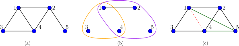
Figure 1: (a) An example of a graph with five vertices. (b) An example of a hypergraph with five vertices. (c) Another graph of five qubits, this graph originates from the graph in (a) by a local complementation on the second vertex. Starting from the second vertex one considers its neighbourhood (the vertices $1,4,$ and $5$) and the corresponding subgraph is inverted. Existing edges ($\{1,4\}$) are removed, and missing ones ($\{1,5\}$ and $\{4,5\}$) are created. See text for further details.

Given a hypergraph $H$ with $N$ vertices we can associate to it a pure quantum state on $N$ qubits in the following way: Any vertex corresponds to a qubit and any qubit is prepared in the state $|+\rangle=(|0\rangle+|1\rangle)/\sqrt{2}$. Then, one applies for each edge a multi-qubit phase gate. For an edge $e$ containing $k$ vertices, this gate is given by

$$C_{e}=\mathbbm{1}_{e}-2|\underbrace{1,\dots,1}_{k\;\;{\rm times}}\rangle\!\langle\underbrace{1,\dots,1}_{k\;\;{\rm times}}|$$ (1)

and acts on the qubits connected by $e$. The phase gate $C_{e}$ acts trivially on all other qubits. So, if we have an element of the computational basis, this vector acquires a sign flip, if and only if it has only $1$-s on every qubit contained in $e$. The hypergraph state is the state after application of all phase gates,

$$|H\rangle=\big{(}\prod_{e\in H}C_{e}\big{)}|+\rangle^{\otimes N}.$$ (2)

Note that all the phase gates commute, so the order of the product does not matter here.

It is convenient that hypergraph states coincide with states which have real and equal weights for any member of the computational basis [3]. These states can be written as

$$|\psi\rangle=\frac{1}{\sqrt{2^{N}}}\sum_{x\in\{0,1\}^{N}}(-1)^{f(x)}|x\rangle,$$ (3)

where $f(x)\in\{0,1\}$. A further very useful fact about hypergraph states is that they can be described by a (non-local) stabilizer. This means that there exists an abelian group of $2^{N}$ observables $S_{i}$ and the hypergraph state is the unique eigenstate of all these observables, that is $S_{i}|H\rangle=|H\rangle$ for all $i$. This offers an alternative definition of hypergraph states, but this is not so important for our approach. For the case of usual graph states, the stabilizer is local, that is, the $S_{i}$ are tensor products of Pauli matrices.

The starting point for our discussion is that different hypergraphs may describe the same hypergraph state up to LU transformations. Let us discuss this first for the special case of graph states. One can ask whether for two different graphs $G_{1}$ and $G_{2}$ the relation

$$|G_{1}\rangle=U_{1}\otimes U_{2}\otimes\dots\otimes U_{N}|G_{2}\rangle$$ (4)

holds. Here, the $U_{i}$ are unitary transformations on the respective qubits. For a small number of qubits ($N\leq 8$) it has turned out that it is sufficient to consider only special unitaries $U_{i}$ from the Clifford group when deciding LU equivalence [1, 18]. These unitaries leave by definition the set of Pauli matrices invariant, i.e., $U\sigma_{i}U^{\dagger}=\pm\sigma_{\pi(i)},$ where $\pi(\cdot)$ is some permutation. This is a discrete set, consisting of elements like $\sigma_{i}$ and $\sqrt{\sigma_{i}}$ and the Hadamard transformation. Moreover, the action of local Clifford (LC) operations graph states has a graphical interpretation in terms of a local complementation of the graph. In this operation, a single vertex is picked and its neighbourhood is inverted, an example is explained in Fig. 1. One can show that this transformation corresponds to an LC transformation on the graph state and, conversely, any LC transformation between graph states can be written as a sequence of local complementations [16].

Of course, given this restricted set of operations with a clear interpretation, it is much easier to decide whether two graph states are LC equivalent. Since LC transformations are sufficient for small systems, it is tempting to conjecture that any LU equivalent pair of graph states is also LC equivalent. This is the LU-LC conjecture. This conjecture is wrong, however, and it is one of the main goals of this paper to develop a systematic procedure to generate counterexamples to this. Concerning LU equivalence of hypergraph states containing edges with three or more vertices, it was shown in Refs. [6, 7] that for $N\leq 4$ all the LU equivalent states are equivalent under a simple application of the Pauli matrices (that is, even a smaller subset than the LC transformations), while for $N\geq 5$ this is not the case [24]. Still many open questions remain. For instance, LU transformations between graph states and hypergraph states have not been identified so far. We will later present an example of a graph state and a hypergraph state containing three-edges, which are LU equivalent.

Let us finally discuss weighted hypergraph states, as they are a main tool to formulate our graphical rules later. Instead of the multiqubit phase gate in Eq. (1) we consider the generalization with an arbitrary phase,

$$C_{e}^{\alpha_{e}}=\mathbbm{1}_{e}-(1-e^{i\pi\alpha_{e}})|\underbrace{1,\dots,1}_{k\;\;{\rm times}}\rangle\!\langle\underbrace{1,\dots,1}_{k\;\;{\rm times}}|.$$ (5)

For $\alpha_{e}=1$ this is just the phase gate from above. Then, the weighted hypergraph state is defined as

$$|H\rangle=\big{(}\prod_{e\in H}C_{e}^{\alpha_{e}}\big{)}|+\rangle^{\otimes N}$$ (6)

and it can be represented by a hypergraph where each edge carries the weight $\alpha_{e}$. We can also express the weighted hypergraph state as a (not necessarily real) equally weighted state

$$|\psi\rangle=\frac{1}{\sqrt{2^{N}}}\sum_{x\in\{0,1\}^{N}}e^{i\pi f(x)}|x\rangle.$$ (7)

Contrary to Eq. (3) the values of the function $f(x)$ are not necessarily in $\{0,1\}$, but can be any real values.

These equally weighted states were originally invented as LME states due to their property of being maximally entangleable to auxiliary systems using only local operations [22]. We will see that the actions of powers of Pauli gates to hypergraph states will in general give us such an LME state. Thus LME states are the fundamental objects if one wishes to study unitary transformations of graph states or hypergraph states.

3 The power of a single-qubit gate

In this section we derive some facts about the power $G^{\alpha}$ of some single-qubit unitary $G$ for an arbitrary real $\alpha$. This will be needed later for giving the LU transformation a graphical description.

We consider unitary operators $G$ that satisfy the condition $G^{2}=\mathbbm{1}$. This condition is equivalent to the statement that $G$ is also a hermitian operator, or alternatively to the statement that all eigenvalues of $G$ are $\pm 1$. Such operators obey the following formula:

$$G=e^{i\pi\frac{\mathbbm{1}-G}{2}}.$$ (8)

From this formula it is natural to define $G^{\alpha}$ for any real $\alpha$ as:

$$G^{\alpha}\equiv e^{i\pi\alpha\frac{\mathbbm{1}-G}{2}}=\frac{1}{2}\big{[}(1+e^{i\pi\alpha})\mathbbm{1}+(1-e^{i\pi\alpha})G\big{]}.$$ (9)

Note that even for scalars non-integer powers are not uniquely defined, thus it is natural that the same occurs with matrices. For example, each Pauli matrix squares to the identity matrix and thus could be considered to be $\mathbbm{1}^{\frac{1}{2}}$. The definition above, however, chooses one particular option out of all possible choices for $G^{\alpha}$.

This definition has some natural properties of usual exponentiation. For example as one would expect: $G^{1}=G$ and $G^{n}$ defined this way coincides with the usual definition of integer powers of a matrix. This definition also coincides with the definition of $C_{e}^{\alpha_{e}}$ for weighted hypergraph states. Moreover, the following equation holds:

$$G^{\alpha_{1}}G^{\alpha_{2}}=G^{\alpha_{1}+\alpha_{2}}\quad\mbox{ for all }\alpha_{1},\alpha_{2}.$$ (10)

It is important, however, to realize that in general the power of a product of matrices $G_{1}$ and $G_{2}$ does not always coincide with product of powers, even if $G_{1}$ and $G_{2}$ commute,

$$(G_{1}G_{2})^{\alpha}\neq G_{1}^{\alpha}G_{2}^{\alpha}.$$ (11)

This is because our definition selects one option out of several for defining the power of a matrix. To give an example that is useful later, we consider single-qubit phase gates

$$C_{1}=\begin{bmatrix}1&0&0&0\\ 0&1&0&0\\ 0&0&-1&0\\ 0&0&0&-1\end{bmatrix}\quad\text{and}\quad C_{2}=\begin{bmatrix}1&0&0&0\\ 0&-1&0&0\\ 0&0&1&0\\ 0&0&0&-1\end{bmatrix},$$ (12)

acting on a two-qubit system. Then the product of their powers and the power of their products can be expressed as follows:

$$C_{1}^{\alpha}\cdot C_{2}^{\alpha}=\begin{bmatrix}1&0&0&0\\ 0&e^{i\pi\alpha}&0&0\\ 0&0&e^{i\pi\alpha}&0\\ 0&0&0&e^{i\pi 2\alpha}\end{bmatrix}\quad(C_{1}\cdot C_{2})^{\alpha}=\begin{bmatrix}1&0&0&0\\ 0&e^{i\pi\alpha}&0&0\\ 0&0&e^{i\pi\alpha}&0\\ 0&0&0&1\end{bmatrix}.$$ (13)

Thus we need the two-qubit phase gate $C_{\{1,2\}}^{-2\alpha}$ as a correction term to obtain $(C_{1}C_{2})^{\alpha}$ from $C_{1}^{\alpha}\cdot C_{2}^{\alpha}$, where

$$C_{\{1,2\}}=\begin{bmatrix}1&0&0&0\\ 0&1&0&0\\ 0&0&1&0\\ 0&0&0&-1\end{bmatrix}\quad\text{and thus}\quad C_{\{1,2\}}^{-2\alpha}=\begin{bmatrix}1&0&0&0\\ 0&1&0&0\\ 0&0&1&0\\ 0&0&0&e^{-i\pi 2\alpha}\end{bmatrix}.$$ (14)

In this example, we have seen that powers of single-qubit operators naturally lead to weighted multi-qubit unitaries. In the following section, we will see a more general formula for powers of such product operators.

4 A graphical rule for the action of $X^{\alpha}$ on a hypergraph state

In this section, we formulate graphical rules for the action of some local unitaries on hypergraph states. We consider powers of the Pauli matrices $\sigma_{x},\sigma_{y}$ and $\sigma_{z}.$ From now on, we will abbreviate the Pauli matrices simply by $X,Y$, and $Z$.

First, if the Pauli $Z$ gate acts on qubit $i$ with some power $\alpha$, the action of $Z_{i}^{\alpha}=C_{i}^{\alpha}$ to the hypergraph state is easy to describe in terms of a weighted hypergraph. Such gates just add weight $\alpha$ to the edge $e=\{i\}$ that contains the single qubit $i$. On the other hand, the Pauli gate $Y^{\alpha}$, in general, does not transform hypergraph states into hypergraph states, it leads out of the space of weighted hypergraph states.

So let us focus on the Pauli $X$ gate. With the power $\alpha=1$ it always transforms hypergraph states into hypergraph states and its effects are well known [6, 4]. Specifically, applied to the $i$-th qubit of the hypergraph state $|H\rangle=(\prod_{e\in H}C_{e})|+\rangle^{\otimes N}$ it produces the state $C_{\Delta_{i}H}|H\rangle$ where $C_{\Delta_{i}H}$ is a diagonal unitary operator defined as follows: $C_{\Delta_{i}H}$ causes the appearance (or disappearance if they are already present) of all edges in the hypergraph $\Delta_{i}H$. The hypergraph $\Delta_{i}H$ is formed by taking all edges in $H$ that contain the vertex $i$ and removing the vertex $i$ from each of them,

$$\Delta_{i}H =\{e-\{i\}\;|\;i\in e,e\in H\}$$

$$=\{e^{\prime}\subseteq\{1,\dots N\}\;|\;i\notin e^{\prime},e^{\prime}\cup\{i\}\in H\},$$ (15)

$$C_{\Delta_{i}H} =\prod_{e\in\Delta_{i}H}C_{e}.$$ (16)

The proof of this rule follows from the commutation relations between the $X_{i}$ and the phase gates $C_{e}$, see Ref. [6] for many examples of this rule.

Let us now consider the action of the $X_{i}^{\alpha}$ gate on a hypergraph state $|H\rangle$. Since $X_{i}^{\alpha}$ can be decomposed into a weighted sum of $\mathbb{1}$ and $X_{i}$ gates, its action on $|H\rangle$ state is easy to characterize:

$$X_{i}^{\alpha}|H\rangle =X_{i}^{\alpha}C_{H}|+\rangle^{\otimes N}$$

$$=\frac{1}{2}\big{[}(1+e^{i\pi\alpha})\mathbb{1}+(1-e^{i\pi\alpha})X_{i}\big{]}C_{H}|+\rangle^{\otimes N}$$

$$=\frac{1}{2}C_{H}\big{[}(1+e^{i\pi\alpha})\mathbb{1}+(1-e^{i\pi\alpha})C_{\Delta_{i}H}X_{i}\big{]}|+\rangle^{\otimes N}$$

$$=\frac{1}{2}C_{H}\big{[}(1+e^{i\pi\alpha})\mathbb{1}+(1-e^{i\pi\alpha})C_{\Delta_{i}H}\big{]}|+\rangle^{\otimes N}$$

$$=C_{\Delta_{i}H}^{\alpha}C_{H}|+\rangle^{\otimes N}=C_{\Delta_{i}H}^{\alpha}|H\rangle.$$ (17)

Thus we see that the result of $X_{i}^{\alpha}$ acting on $|H\rangle$ is the same as the result of $C_{\Delta_{i}H}^{\alpha}$ acting on $|H\rangle$,

$$(X_{i})^{\alpha}|H\rangle=(C_{\Delta_{i}H})^{\alpha}|H\rangle.$$ (18)

To understand the graphical interpretation of this action, we need to look at $C_{\Delta_{i}H}^{\alpha}$ and decompose it into actions of gates that change the weight of single hyperedges. In general, $C_{\Delta_{i}H}$ is a product of several hyperedge gates, $C_{\Delta_{i}H}=C_{e_{1}}C_{e_{2}}\ldots C_{e_{k}}$, and for taking the power we have to recall that $(G_{1}G_{2})^{\alpha}\neq G_{1}^{\alpha}G_{2}^{\alpha}$. Thus we need to study the decomposition of powers of products of individual edge producing gates.

To calculate $C_{\Delta_{i}H}^{\alpha}$, we need to look at the eigenspace of $C_{\Delta_{i}H}$ with eigenvalue $-1$ and change its eigenvalue to $e^{i\pi\alpha}$. Since $C_{\Delta_{i}H}$ is diagonal in the computational basis, this eigenspace is spanned by vectors in the computational basis. In fact, it is spanned by all vectors in the computational basis that are contained in the symmetric difference (denoted by $\bigoplus$) of the $-1$ eigenspace basis-vectors of all the edges in $\Delta_{i}H$. We can compute the indicator function ${\rm\bf I}_{\bigoplus_{i=1}^{k}e_{i}}$ of the symmetric difference of $k$ sets using a formula similar to the inclusion-exclusion principle,

$${\rm\bf I}_{\bigoplus_{i=1}^{k}e_{i}}=\sum_{S\subseteq\{1,2\ldots k\},S\neq\emptyset}(-2)^{|S|-1}{\rm\bf I}_{\bigcup\limits_{j\in S}e_{j}}.$$ (19)

Using this formula, we can obtain an expression for powers of products of $C_{e}$ gates. The simplest case was already discussed in the previous section:

$$(C_{e_{1}}C_{e_{2}})^{\alpha} =C_{e_{1}}^{\alpha}C_{e_{2}}^{\alpha}C_{e_{1}\cup e_{2}}^{-2\alpha},$$ (20)

$$(C_{e_{1}}C_{e_{2}}C_{e_{3}})^{\alpha} =C_{e_{1}}^{\alpha}C_{e_{2}}^{\alpha}C_{e_{3}}^{\alpha}C_{e_{1}\cup e_{2}}^{-2\alpha}C_{e_{1}\cup e_{3}}^{-2\alpha}C_{e_{2}\cup e_{3}}^{-2\alpha}C_{e_{1}\cup e_{2}\cup e_{3}}^{4\alpha},$$ (21)

and generally

$$\big{(}\prod\limits_{i=1}^{k}C_{e_{i}}\big{)}^{\alpha} =\prod\limits_{S\subseteq\{1,2\ldots k\},S\neq\emptyset}(C_{\bigcup\limits_{j\in S}e_{j}})^{(-2)^{|S|-1}\alpha}.$$ (22)

Thus the effect of the $X^{\alpha}$ gate on qubit $i$ in a hypergraph state $|H\rangle$ is the following:

• For each edge $e^{\prime}$ in $\mathcal{A}_{i}=\{e^{\prime}\subset\{1,\dots,N\}|i\notin e^{\prime},e^{\prime}\cup\{i\}\in H\}$ add weight $\alpha$ to the edge $e^{\prime}$ in the hypergraph.

• For each pair of edges $\{e_{1},e_{2}\in\mathcal{A}_{i}|e_{1}\neq e_{2}\}$ subtract weight $2\alpha$ from edge $e_{1}\cup e_{2}$

• For each triplet of distinct edges $\{e_{1},e_{2},e_{3}\in\mathcal{A}_{i}\}$ add weight $4\alpha$ to the edge $e_{1}\cup e_{2}\cup e_{3}$

• In general: For each $k$-tuple of distinct edges in $e_{1}\ldots e_{k}\in\mathcal{A}_{i}$ add weight $(-2)^{k-1}\alpha$ to the edge $\cup_{j=1}^{k}e_{j}.$

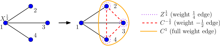
Figure 2: An example for the graphical action of the $X^{\alpha}$ gate. The action of $X^{\frac{1}{4}}$ gate on the first qubit of the four-qubit star graph produces three single-qubit edges $\{2\},\{3\}$ and $\{4\}$ with weights $\frac{1}{4}$, three two-qubit edges $\{2,3\},\{2,4\}$ and $\{3,4\}$ with weight $-\frac{1}{2}$ and a single full-weight three-qubit hyperedge $\{2,3,4\}$.

An example of these rules is shown in Fig. 2. We can easily see that if $\alpha=1$ all the terms with unions of two or more edges add weight that is a multiple of two. Since $C_{e}^{2}=\mathbb{1}$ we only need to consider the weight modulo two, so these terms act trivially on the hypergraph. The remaining terms correctly describe the action of Pauli $X$ gate on the hypergraph.

When $\alpha=\frac{1}{2}$, all the terms with triple or larger unions add weight that is a multiple of two and thus act trivially. Therefore only terms with single edges and pairs of edges remain. If we look at the effect graphically we can see that this corresponds (up to some single-vertex actions of weight $1/2$) to the local complementation operation of the graph state around vertex $i$ (see Fig. 1). This is again to be expected, since $X^{\frac{1}{2}}$ is (up to some single qubit terms $Z^{\frac{1}{2}}$) the gate that performs local complementation for graph states.

For other values of $\alpha$ we can obtain interesting examples of transformations of graph and hypergraph states. Some of these can be obtained using Clifford gates only, but some others require the use of non-Clifford gates. Such examples, along with proofs that they cannot be obtained using Clifford transformations, are described in following sections.

5 Graph states and hypergraph states can be LU equivalent

In order to see how our graphical rule is useful, we now describe an example of a hypergraph state that is LU equivalent to a normal graph state. The trick that we use is later relevant for constructing counterexamples to the LU-LC conjecture.

We have seen already in Fig. 2 how a $X^{\frac{1}{4}}$ gate can create a three-edge acting on a graph state, but we also created some other edges with fractional weights. To obtain a pure hypergraph state with no fractional weight edges, we will need to cancel the fractional edges by other fractional power gates. Consider an example where we have a four-qubit star graph as before, but now each pair of non-central qubits is also connected to a different vertex. As shown on Fig. 3, if we apply $X^{\frac{1}{4}}$ on the central qubit of the star graph, we obtain a three-hyperedge with several fractional two-edges and one-edges.

Figure 3: The first stage of transformation of a pure graph state into a hypergraph state with a three-edge. See text for further details.

However, as demonstrated in Fig. 4 we can cancel the partial two-edges by applying $X^{-\frac{1}{4}}$ on the three qubits that connected to pairs of affected vertices. These gates will cancel the two-edges, but since two of them add weight $-\frac{1}{4}$ to every single-qubit edge, each single-qubit edge weight will reverse from $\frac{1}{4}$ to $-\frac{1}{4}.$

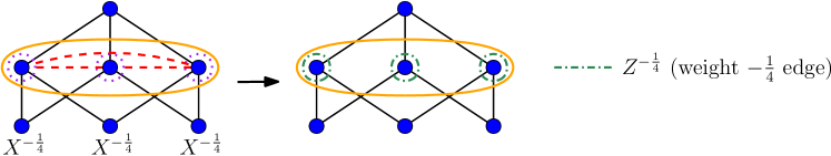
Figure 4: In the second stage, one has to cancel the partial two-edges that appeared after the first stage. This is done by applying $X^{-\frac{1}{4}}$ gates to the qubits on the bottom.

This leaves us nearly with a hypergraph state, we only need to cancel the fractional single qubit edges. For this we can just use local $Z^{\frac{1}{4}}$ gates on those qubits and obtain a hypergraph state. Fig. 5 combines all three steps and shows how a graph state can be transformed into a hypergraph state with a three-edge. Since LC actions cannot transform a graph state into a hypergraph states, this gives us an example of two hypergraph states that are LU equivalent, but not LC equivalent.

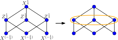
Figure 5: Complete transformation of a pure graph state into a hypergraph state via local unitary transformations.

6 Generating counterexamples to the LU-LC conjecture

In this section we will show how to systematically generate pairs of graph states that are LU equivalent, but not LC equivalent. These are then counterexamples to the LU-LC conjecture. We will show how to construct an example with $28$ qubits, but our example generalises to more qubits. In the following section, we will also construct a counterexample with 27 qubits, but the construction with 28 qubits is simpler, so we explain it first.

Consider the graph $G_{1}$ from Fig. 6. This is a bipartite graph with seven vertices on one side (the “left” side) and $\binom{7}{5}=21$ vertices on the other side (the “right” side). Each vertex on the right side corresponds to a set of five vertices on the left side and is connected with an edge to exactly those five vertices. For a possible generalization, an analogous construction with $n=8k-1$ vertices on the left side and $\binom{n}{5}$ vertices on the right side works as well. We can also obtain a similar construction if we take $n=8k-1$ vertices on the left side and $\binom{n}{4}$ vertices on the right, each of which is connected to a unique set of four vertices on the left. But for the sake of simplicity we consider the graph from Fig. 6 in the following.

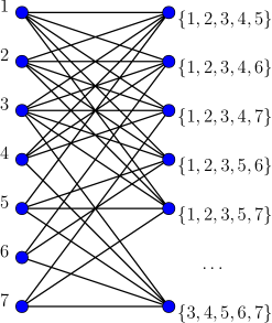
Figure 6: A bipartite graph construction with seven vertices on the left side and $21=\binom{7}{5}$ vertices on the right side. Each of the vertices on the right side is connected to a five-vertex subset of the vertices on the left side. This construction is used to find counterexamples to the LU-LC conjecture, see text for further details.

Let us see what happens if we perform $X^{\frac{1}{4}}$ on every vertex on the right side:

• Each single-qubit edge on the left side will appear with weight $\frac{1}{4}$, multiplied with the number of neighbours the qubit has (which is $\binom{6}{4}=15$). Thus we will have all single-qubit edges with weights of $\frac{15}{4}$, but we can easily cancel these by applying the $Z^{-\frac{15}{4}}$ gates to every qubit on the left side.

• Each two-edge between vertices on the left side will appear with weight $-\frac{1}{2}$, multiplied with the number of qubits on the right that are connected to both of the ends of such an edge. The number of such qubits on the right is $\binom{7-2}{5-2}=\binom{5}{3}=10$, thus every edge will appear with weight $-5$, which is equivalent to $1$ modulo $2$. Thus we will make every possible two-edge on the left side appear.

• Each three-edge will appear with weight $1$, multiplied with the number of qubits on the right that are connected to all three qubits in the edge. There are $\binom{7-3}{5-3}=\binom{4}{2}=6$ such qubits. Thus the three-edge will appear with weight $6$, which is equivalent to not appearing at all, since the weights are counted modulo $2$.

• All four-edges and five-edges appear with weights that are multiples of $2$, which is also equivalent to not appearing at all.

Thus the graph state of the bipartite graph $G_{1}$ described above is LU equivalent to the graph state of graph $G_{2}$, which has the same edges between the two parts as $G_{1}$ and also has no edges between vertices on the right side but, unlike $G_{1}$, all the vertices of $G_{2}$ on the left side are connected to each other.

Now we need to show that $G_{2}$ cannot be obtained from $G_{1}$ by local Clifford operations only. It has been shown [16] that any Clifford transformation can be decomposed into a series of local complementation operations on the graph state. Using this fact, we break our proof into two parts.

1. First we show that $G_{2}$ cannot be obtained from $G_{1}$ using only local complementation operations on vertices in the right hand side of the graph.

2. Then we show a general Lemma, stating that if we can obtain a graph state $G_{2}$ from a bipartite graph state $G_{1}$, and $G_{2}$ only differs from $G_{1}$ by edges between vertices on the left side, then it must be the case that local complementations of the right side suffice to produce the transformation. Together with the first part this will complete the proof.

First part of the proof. —

The first part of the proof is quite simple. We only need to observe that each local complementation operation on vertices in the right-hand side affects $\binom{5}{2}=10$ edges. Since that is an even number, the parity of the number of edges on the left always remains even (as it started from the even number zero). Thus, it must be even at the end of the transformation. However, $\binom{7}{2}=21$ is an odd number. This shows that we can never obtain all edges on the left-hand side using only local complementations on the right side.

Second part of the proof. —

In this part we to show that if the graph state $|G_{2}\rangle$ can be obtained from $|G_{1}\rangle$ using Clifford operations, then there must be a set of vertices on the right side, such that $G_{1}$ is transformed into $G_{2}$ by performing local complementation operations on exactly those vertices. We will show this by proving a more general fact that works for almost any bipartite $G_{1}$, that is, any graph $G_{1}$ that can be divided into two sides with edges running only from one side to another and never within one side. We will also use the fact that there is a path from every vertex to every other vertex in $G_{1}$, which means that $G_{1}$ is connected. The mathematical result is the following:

Lemma. Let $G_{1}$ be a connected bipartite graph that has $k_{1}$ vertices on the left side of the bipartition and $k_{2}$ on the right side, with $k_{1}\neq k_{2}$. Let $G_{2}$ be a graph with the same vertices and the same edges between the two sides, but some extra edges added on the left side of the graph. Then, if the graph state $|G_{1}\rangle$ can be transformed into graph state $|G_{2}\rangle$ using local Clifford gates, the graph $G_{1}$ can be transformed into $G_{2}$ using local complementation applied to vertices on the right side only.

Proof. It has been shown in Ref. [16] that whether two graph states are equivalent under LC operations can be determined using a set of equations over the binary field. Specifically, let us consider the stabiliser matrices $S_{1}$ and $S_{2}$ of the corresponding graphs $G_{1}$ and $G_{2}$ as $2n\times n$ matrices, where $n$ is the total number of vertices in each graph. These matrices have the adjacency matrix of the corresponding graph in the top part and the identity matrix in the bottom part, i.e.,

$$S_{1}=\begin{bmatrix}\theta_{1}\\ \mathbbm{1}\end{bmatrix},\quad S_{2}=\begin{bmatrix}\theta_{2}\\ \mathbbm{1}\end{bmatrix},$$ (23)

with $\theta_{1}$ and $\theta_{2}$ being the adjacency matrices of the corresponding graphs. Then the graph states $|G_{1}\rangle$ and $|G_{2}\rangle$ are LC equivalent if and only if there exists a binary matrix $Q$ of size $2n\times 2n$ with a block structure

$$Q=\begin{bmatrix}A&B\\ C&D\end{bmatrix},$$ (24)

where $A$, $B$, $C$ and $D$ are diagonal and satisfy the following equations:

$$A_{ii}D_{ii}+B_{ii}C_{ii}=1\quad\mbox{ for all }i$$ (25)

and

$$S_{1}^{T}\cdot Q^{T}\cdot\begin{bmatrix}0&\mathbb{1}\\ \mathbb{1}&0\end{bmatrix}\cdot S_{2}=0.$$ (26)

Substituting $S_{1}$ and $S_{2}$ into Eq. (26) we obtain the following criterion:

$$\theta_{1}C\theta_{2}+\theta_{1}A+D\theta_{2}+B=0.$$ (27)

In our case the first graph $G_{1}$ is bipartite and the second one is obtained from the first one by adding some edges on one side of the graph. Thus the matrices $\theta_{1}$ and $\theta_{2}$ have the following special forms:

$$\theta_{1}=\begin{bmatrix}0&\zeta\\ \zeta^{T}&0\end{bmatrix},\quad\theta_{2}=\begin{bmatrix}\eta&\zeta\\ \zeta^{T}&0\end{bmatrix},$$ (28)

where $\eta$ is the adjacency matrix of the subgraph on the left side generated by the transformation, and $\zeta$ is an $k_{1}\times k_{2}$ matrix that shows which vertices on the left side are adjacent to which ones on the right side. We also use the fact that, since all of $A$, $B$, $C$ and $D$ are diagonal, they can be written as:

$$A=\begin{bmatrix}A_{u}&0\\ 0&A_{l}\end{bmatrix},\quad B=\begin{bmatrix}B_{u}&0\\ 0&B_{l}\end{bmatrix},\quad C=\begin{bmatrix}C_{u}&0\\ 0&C_{l}\end{bmatrix},\quad D=\begin{bmatrix}D_{u}&0\\ 0&D_{l}\end{bmatrix},$$ (29)

with all the nonzero upper parts sized $k_{1}\times k_{1}$ and all the nonzero lower parts sized $k_{2}\times k_{2}$.

Then, Eq. (27) gives us the following condition:

$$\begin{bmatrix}\zeta C_{l}\zeta^{T}&0\\ \zeta^{T}C_{u}\eta&\zeta^{T}C_{u}\zeta\end{bmatrix}+\begin{bmatrix}0&\zeta A_{l}\\ \zeta^{T}A_{u}&0\end{bmatrix}+\begin{bmatrix}D_{u}\eta&D_{u}\zeta\\ D_{l}\zeta^{T}&0\end{bmatrix}+\begin{bmatrix}B_{u}&0\\ 0&B_{l}\end{bmatrix}=\begin{bmatrix}0&0\\ 0&0\end{bmatrix}.$$ (30)

Thus we have four matrix equations over the binary field:

$$\zeta C_{l}\zeta^{T}+D_{u}\eta+B_{u}=0,$$ (31)

$$\zeta A_{l}+D_{u}\zeta=0,$$ (32)

$$\zeta^{T}C_{u}\eta+\zeta^{T}A_{u}+D_{l}\zeta^{T}=0,$$ (33)

$$\zeta^{T}C_{u}\zeta+B_{l}=0.$$ (34)

Let us analyse Eq. (32) first. Since both $A_{l}$ and $D_{u}$ are diagonal, the terms $\zeta A_{l}$ and $D_{u}\zeta$ correspond to some selections of columns and rows of $\zeta$ respectively. These two terms need to sum to zero, which is the same as being equal over the binary field. But for every $i$, such that $(A_{l})_{ii}=1$ we have a full column $i$ of $\zeta$ in $\zeta A_{l}$, and thus for every position $j$ where $\zeta_{ij}=1$ we must also have the $j$-th row in $D_{u}\zeta$. Therefore, we need to have $(D_{u})_{jj}=1$. In graph theoretic terms, whenever we have $(A_{l})_{ii}=1$ we need to have $(D_{u})_{jj}=1$ for every vertex $j$ that is connected to $i$. Similarly, whenever we have $(D_{u})_{jj}=1$, we must have $(A_{l})_{ii}=1$ for every vertex $i$ connected to $j$. But since the whole graph is connected, the matrices $A_{l}$ and $D_{u}$ must simultaneously both be zero matrices or both be identity matrices of their respective dimensions. Hence, we have two cases to consider:

Case 1: If $A_{l}=0_{k_{2}\times k_{2}}$ and $D_{u}=0_{k_{1}\times k_{1}}$ the term $A_{ii}D_{ii}$ is zero for all $i$ both in the upper and in the lower parts of the matrix. Thus $B_{ii}C_{ii}$ has to be one everywhere, meaning that $B_{u}=C_{u}=\mathbbm{1}_{k_{1}\times k_{1}}$ and $B_{l}=C_{l}=\mathbbm{1}_{k_{2}\times k_{2}}$. Then Eq. (31) gives us $\zeta\zeta^{T}=\mathbbm{1}_{k_{1}\times k_{1}}$, and Eq. (34) gives us $\zeta^{T}\zeta=\mathbbm{1}_{k_{2}\times k_{2}}$. But this cannot be: $\zeta$ and $\zeta^{T}$ are rectangular matrices and cannot have rank more than the $\min(k_{1},k_{2})$. This means that $\zeta^{T}\zeta$ and $\zeta\zeta^{T}$ must also have rank no higher than $\min(k_{1},k_{2})$ and since $k_{1}\neq k_{2}$ this contradicts at least one of the equations $\zeta\zeta^{T}=\mathbbm{1}_{k_{1}\times k_{1}}$ or $\zeta^{T}\zeta=\mathbbm{1}_{k_{2}\times k_{2}}$. Thus this Case 1 cannot happen.

Case 2: If $A_{l}=\mathbbm{1}_{k_{2}\times k_{2}}$ and $D_{u}=\mathbbm{1}_{k_{1}\times k_{1}}$ the Eq. (31) simplifies to the condition $\zeta C_{l}\zeta^{T}=\eta+B_{u}$. Let us look what happens to the adjacency matrix if we apply local complementation on vertex $j$ on the right side. This changes the matrix $\eta$. As we know, we affect edges that connect pairs of vertices neighbouring vertex $j$. Thus the part $\eta$ of the adjacency matrix will change by the matrix $\zeta O_{j}\zeta^{T}$ (up to a diagonal correction), where $O_{j}$ is a matrix with zeros everywhere except on the $j$-th entry of the diagonal, which contains a $1$.

Let us take the set of vertices $j$ on the right side, such that $(C_{l})_{jj}=1$. If we start from graph $G_{1}$ and apply local complementation to exactly those vertices, then we produce the following adjacency matrix on the left:

$$\zeta O_{j_{1}}\zeta^{T}+\zeta O_{j_{2}}\zeta^{T}+\ldots+\zeta O_{j_{m}}\zeta^{T}=\zeta C_{l}\zeta^{T}.$$ (35)

Thus we obtain the adjacency matrix $\eta$ (up to a diagonal correction, parametrized by $B_{u}$) using local complementations on the vertices $j$ with $(C_{l})_{jj}=1$ the right side. Since local complementations produce graph states from graph states the diagonal entries of $\eta$ and our resulting adjacency matrix will also match. Thus as we wanted to show, if there is any LC transformation that produces the graph state with the desired form, then local complementations on vertices in the right side suffice for such a transformation. $\hfill\Box$

This theorem completes the proof that the examples of LU equivalent graph states from above cannot be transformed into each other by means of LC transformations. Note that we did not need the lower right side of the adjacency matrix $\theta_{1}$ to be zero. Thus our proof could be generalised to the case when the initial graph is not bipartite, but has some edges connecting right side qubits to each other. However we still need to require that the final graph has no edges connecting right side qubits to each other. In this case we would see that any local Clifford transformation could be achieved by first cancelling the edges on the right side using local complementations on the left and then creating the edges on the left side by using local complementations on the right. However, our construction does not need such a generalised version of the theorem.

7 A counterexample to the LU-LC conjecture with 27 qubits

So far, we have presented a family of counterexamples to the LU-LC conjecture, the smallest one having 28 qubits. In the literature, however, the smallest explicit counterexample has 27 qubits and has been found by numerical search [21]. So, one may ask whether our construction and the known example are related.

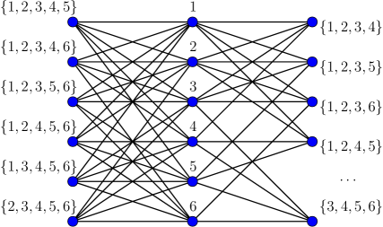
Figure 7: The counterexample to the LU-LC conjecture for 27 qubits. The graph has six central vertices, $6=\binom{6}{5}$ vertices on the right-hand side and $15=\binom{6}{4}$ vertices on the left side. Applying $X^{\frac{1}{4}}$ on all qubits on the right side and on the left side induces all possible connections between the central vertices, i.e. the central subgraph becomes fully connected. This cannot be achieved by local complementation.

Indeed, with our methods we can directly construct the known counterexample and understand why it is a counterexample. Consider the graph with 27 vertices shown in Fig. 7. This is a slight modification of the graph in Fig. 6 discussed before. It is a bipartite graph with six vertices (the central vertices) in one part of the bipartition and 21 vertices (the left and the right vertices) in the other part. As before, one can directly verify the following facts:

• If we apply $X^{\frac{1}{4}}$ on all the $21$ qubits on the right-hand side and one the left-hand side, any possible two-edge between the central qubits will be created with weight one. Higher-order edges will not be created. In addition, any single-qubit edge on the central qubits will occur with weight $15/4$, but this can be corrected by local $Z$ gates on the central qubits.

• The number of created two-edges on the central qubits is $15=\binom{6}{2}$, which is odd. This cannot be created by local complementation using qubits on the right side or the left side, since each of these local complementations changes an even number of edges (either $10=\binom{5}{2}$ or $6=\binom{4}{2}$) on the central qubits.

• Finally, the Lemma from the previous section proves that it is sufficient to consider these special local complementations.

So, the graph in Fig. 7 is a counterexample to the LU-LC conjecture. The graph before and after this transformation is also shown in Fig. 8 (a) and (b).

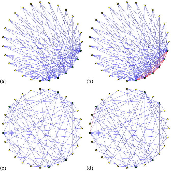
Figure 8: The relation between the different counterexamples to the LU-LC conjecture for 27 qubits. (a) The graph from Fig. 7 which forms the starting point of our considerations. This is a bipartite graph, the bipartition is highlighted by the yellow and green vertices. (b) After applying LU transformations to the graph in (a), the central qubits become connected (shown in red). (c) The graph from Ref. [21], which was used there as a starting point. This is also a bipartite graph, the bipartition is highlighted by the yellow and dark green vertices. The graphs (a) and (c) are equivalent under local complementation without any additional permutation. (d) As shown in Ref. [21], after LU transformations on the graph (c) a single edge (shown in red) can be created. But the graphs (c) and (d) are not LC equivalent. Now, (b) and (d) are equivalent under local complementation, without any permutation.

It remains to show that this example is equivalent to the example from Ref. [21]. The adjacency matrix is explicitly given in that reference, so one may be tempted to check the LC equivalence directly by solving the equations over the binary field as outlined in the previous section [16, 17]. This, however, is not feasible, as there are $27!\approx 10^{28}$ permutations of the vertices which have to be taken into account. Nevertheless one can find the sequence of local complementations and permutations using the following ideas:

• The first observation is that the graph from Ref. [21] is bipartite, also with six vertices on the one side and 21 vertices on the other side.

• The second observation is that certain types of sequences of local complementations of the graph from Fig. 7 do not change the property that it is bipartite, but the partition changes. For instance, if we perform a local complementation on the six central vertices, then the local complementation on some other vertices $\{a,b,c,\dots\}$ on the other side, then local complementation on the six central vertices again, and finally on the vertices $\{a,b,c,\dots\}$ again, the graph typically stays bipartite (again with a $6$ vs. $21$ splitting), but the qubits are permuted and the two parts have changed.

• Considering such transformations, one finds with some exhaustive search transformations which transform the graph from Fig. 7 to a graph with the same degree distribution as the graph from Ref. [21]. More specifically, the set $\{a,b,c,\dots\}$ consists of six qubits, four on the right side and two on the left side. For these transformations and with the help of the given degree distribution one finds a final permutation to map one graph to the other.

With this method we were able to show that under local complementation the initial state in Ref. [21] is equivalent to our state from Fig. 7, and the final state from Ref. [21] is also equivalent to our final state. The corresponding graphs are also displayed in Fig. 8 and a Mathematica file with the explicit calculation is contained in the supplementary information [25]. This proves that our method explains the numerically found counterexample from Ref. [21].

The example with 27 qubits is the smallest example that we could find with our methods. As stated in Ref. [21], also the numerical search gives as a minimal example the example with 27 qubit. It would be interesting to decide whether this is indeed the smallest possible example.

Finally, we should add that further counterexamples to the LU-LC conjecture have been found by M. Grassl and B. Zeng [26]. They found counterexamples for $N\in\{27,$ $28,$ $35,36,38,39,40,41,42,43,$ $44,45,46,47,48,49,$ $50,51,52,54,55,56,59,60,$ $76,$ $115,116,123,124,131,132\}$ using randomized combinatorial search and methods from coding theory. With our methods, we were not able to find counterexamples for all of these values of $N$. This suggests that our construction is not the only way for generating counterexamples and more refined construction methods may be found.

8 Conclusion

In summary, we have investigated the action of local unitary transformations beyond local Clifford operations on graph states and hypergraph states. For the action of $X_{i}^{\alpha}$ gates we found a graphical rule in terms of weighted hypergraphs. Using this rule, we showed an example where hypergraph states and graph states are locally equivalent. We also provided a method to generate systematically counterexamples to the LU-LC conjecture. This also allowed to understand a previously known counterexample.

For further research, there are several open questions. First, it would be interesting to explore the application of our rule to hypergraph states. For instance, it has been suggested that if one has two hypergraph states where one has only $k$-edges and the other has only $\ell$-edges then they may be locally inequivalent [3]. Our graphical rule may be useful to find counterexamples to this question. Another interesting problem is to find graphical rules for other local transformations. They may not be applicable in all situations, as the transformations may, in general, lead out of the space of weighted hypergraph states. Nevertheless, for a restricted class of states such transformations and rules may be possible.

9 Acknowledgements

We thank Mariami Gachechiladze, Markus Grassl, and David Gross for discussions. This work has been supported by the DFG and the ERC (Consolidator Grant 683107/TempoQ).

References

References

- [1] M. Hein, J. Eisert and H. J. Briegel, Phys. Rev. A 69, 062311 (2004).
- [2] M. Hein, W. Dür, J. Eisert, R. Raussendorf, M. Van den Nest, and H.-J. Briegel, Entanglement in Graph States and its Applications, in Quantum Computers, Algorithms and Chaos, edited by G. Casati, D.L. Shepelyansky, P. Zoller, and G. Benenti (IOS Press, Amsterdam, 2006), quant-ph/0602096.
- [3] M. Rossi, M. Huber, D. Bruß, and C. Macchiavello, New J. Phys. 15, 113022 (2013).
- [4] R. Qu, J. Wang, Z. Li, and Y. Bao, Phys. Rev. A 87, 022311 (2013).
- [5] M. Rossi, D. Bruß, and C. Macchiavello, Phys. Scr. T160, 014036 (2014).
- [6] O. Gühne, M. Cuquet, F. E. S. Steinhoff, T. Moroder, M. Rossi, D. Bruß, B. Kraus, and C. Macchiavello, J. Phys. A: Math. Theor. 47, 335303 (2014).
- [7] X.-Y. Chen and L. Wang, J. Phys. A: Math. Theor. 47, 415304 (2014).
- [8] D. W. Lyons, D. J. Upchurch, S. N. Walck, and C. D. Yetter, J. Phys. A: Math. Theor. 48, 095301 (2015).
- [9] D. W. Lyons, N. P. Gibbons, M. A. Peters, D. J. Upchurch, S. N. Walck, and E. W. Wertz, arXiv:1609.01306.
- [10] M. Gachechiladze, C. Budroni, and O. Gühne, Phys. Rev. Lett. 116, 070401 (2016).
- [11] D. Schlingemann and R.F. Werner, Phys. Rev. A 65, 012308 (2002).
- [12] M. Grassl, A. Klappenecker, and M. Rötteler, Proceedings 2002 IEEE International Symposium on Information Theory (ISIT 2002), Lausanne, Switzerland, June/July 2002, p. 45, quant-ph/0703112.
- [13] H. J. Briegel, D. E. Browne, W. Dür, R. Raussendorf, and M. Van den Nest, Nat. Phys. 5, 19 (2009).
- [14] A. Cabello, A.J. Lopez-Tarrida, P. Moreno, and J.R. Portillo, Phys. Lett. A 373, 2219 (2009); Erratum: Phys. Lett. A 374, 3991 (2010).
- [15] A. Cabello, A.J. Lopez-Tarrida, P. Moreno, and J.R. Portillo, Phys. Rev. A 80, 012102 (2009).
- [16] M. van den Nest, J. Dehaene and B. De Moor, Phys. Rev. A 69, 022316 (2004).
- [17] M. van den Nest, J. Dehaene and B. De Moor, Phys. Rev. A 70, 034302 (2004).
- [18] M. van den Nest, J. Dehaene and B. De Moor, Phys. Rev. A 71, 062323 (2005).
- [19] B. Zeng, H. Chung, A. W. Cross, and I. L. Chuang, Phys. Rev. A 75, 032325 (2007).
- [20] D. Gross and M. Van den Nest, Quantum Inf. Comp. 8, 263 (2008).
- [21] Z. Ji, J. Chen, Z. Wei, and M. Ying, Quantum Inf. Comp. 10, 97 (2010).
- [22] C. Kruszynska and B. Kraus, Phys. Rev. A 79, 052304 (2009).
- [23] T. Carle, B. Kraus, W. Dür, and J.I. de Vicente, Phys. Rev. A 87, 012328 (2013).
- [24] M. Gachechiladze, N. Tsimakuridze, and O. Gühne, J. Phys. A: Math. Theor. 50, 19LT01 (2017).
- [25] The file is also available in the submission files of this paper on the arxiv, see https://arxiv.org/e-print/1611.06938v1.
- [26] M. Grassl, private communication, 2016.