Phase co-existence in bidimensional passive and active dumbbell systems

Abstract

We demonstrate that there is macroscopic co-existence between regions with hexatic order and regions in the liquid/gas phase over a finite interval of packing fractions in active dumbbell systems with repulsive power-law interactions in two dimensions. In the passive limit this interval remains finite, similarly to what has been found in bidimensional systems of hard and soft disks. We did not find discontinuous behaviour upon increasing activity from the passive limit.

Interest in the behaviour of $2d$ (and also $3d$) macroscopic systems under continuous and homogeneous input of energy has been boosted by their connection with active matter Toner et al. (2005); Fletcher and Geissler (2009); Romanczuk et al. (2012); Vicsek and Zafeiris (2012); Cates (2012); Marchetti et al. (2013); de Magistris and Marenduzzo (2015); Elgeti et al. (2015). This new type of matter can be realised in various ways. Systems of self-propelled particles constitute an important subclass, with natural examples such as suspensions of bacteria Wu and Libchaber (2000); Dombrowski et al. (2004); Rabani et al. (2013), and artificial ones made of Janus Paxton et al. (2004); Buttinoni et al. (2013); Ginot et al. (2015) or asymmetric granular Lam et al. (2015) particles. In all these cases, the constituents consume internal or environmental energy and use it to displace. Very rich collective motion arises under these out of equilibrium conditions, and liquid, solid and segregated phases are observed Tailleur and Cates (2008); Fily and Marchetti (2012); Stenhammar et al. (2013); Redner et al. (2013); Wysocki et al. (2014); Weber et al. (2014). In particular, in active Brownian particle systems, segregation, also called motility induced phase separation (MIPS), was claimed to occur only above a large critical threshold of the activity Redner et al. (2013); Stenhammar et al. (2014); Suma et al. (2014a); Marchetti et al. (2016); Redner et al. (2016).

Besides, the behaviour of passive disks is a classic theme of study in soft condensed matter. Recently, Bernard & Krauth argued that $2d$ melting of hard and soft repulsive disks occurs in two steps, with a continuous Berezinskii-Kosterlitz-Thouless transition between the solid and hexatic phases, and a first order transition between the hexatic and liquid phases, when density or packing fraction are decreased at constant temperature Bernard and Krauth (2011). The hexatic phase has no positional order but quasi long-range orientational order, while the solid phase has quasi long-range positional and proper long-range orientational order. Liquid and quasi long-range orientationally ordered zones co-exist close to the liquid phase, within a narrow interval of packing fractions.

In this Letter we study the phase diagram of a bidimensional model of active purely repulsive dumbbells and show that it does not comply with the MIPS scenario. We prove that the phase separation found at high values of the activity continuously links, in the passive limit, to a finite co-existence region as the one predicted by Bernard & Krauth for $2d$ melting of hard and soft repulsive disks Bernard and Krauth (2011). There is no non-vanishing critical value of activity needed for segregation in this system, making the popular MIPS scenario at least not general.

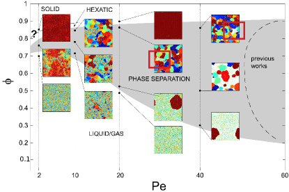
Figure 1: (Color online.) The phase diagram and some representative local hexatic parameter maps. Note the red rectangular contours in the boxes at Pe $=20$ and Pe $=40$ that surround the disordered regions. The way in which the phase boundaries are determined is explained in the text and more details are given in the SM.

The reason for choosing a dumbbell model is that many natural swimmers have elongated shape, and a hard dimer is the simplest approximation of such anisotropy Wojciechowski et al. (1991, 1993); Valeriani et al. (2011). This geometry favours aggregation at intermediate densities and sufficiently strong activation Peruani et al. (2006); Gonnella et al. (2014); Suma et al. (2014a); Cugliandolo et al. (2015); Joyeux and Bertin (2016); Gonnella et al. (2015); Siebert et al. (2016). In this limit the evolution of an initial homogeneous phase occurs by nucleation and growth of clusters Gonnella et al. (2014) and the system phase separates. At the other extreme, for sufficiently low densities and not so strong activity, particles form only very small clusters that do not coalesce Suma et al. (2014b); Cugliandolo et al. (2015); Suma et al. (2015). The results in this Letter complement these two extreme limits. In the absence of activity we confirm the results of Bernard, Kapfer & Krauth for hard and soft disks Bernard and Krauth (2011); Engel et al. (2013); Kapfer and Krauth (2015) –for what concerns the existence of a first-order transition from the liquid phase– using now a molecular system and estimating the density interval for co-existence. We prove that this interval continuously expands towards the strong activity region where cluster aggregation had already been observed. Hence, there is no discontinuity between the passive and active regions in the phase diagram with phase separation. Figure 1 summarises this scenario that, we emphasise, is different from what has been stated in the literature so far. We did not analyze in this work the transition between hexatic and solid phase.

Event-chain algorithms have proven to be an efficient tool to equilibrate $2d$ interacting particle systems Bernard et al. (2009) and they have been used to give strong support to the two step phase transition scenario Bernard and Krauth (2011); Kapfer and Krauth (2015). We use, however, conventional molecular dynamics in order to simulate the out of equilibrium dynamics of active systems as realistically as possibly.

The model consists of $N$ diatomic molecules (dimers) with identical spherical head and tail centered at a fixed distance equal to their diameters, $\sigma_{\rm d}$. Interactions are mediated by a purely repulsive potential, $U(r)=4\epsilon[(r/\sigma)^{-2n}-(r/\sigma)^{-n}]$, truncated at its minimum $r_{c}=2^{1/n}\sigma$, with $r$ the distance between the centers of any two disks. We set $\sigma=2^{-1/n}\sigma_{\rm d}$, so that $r_{c}=\sigma_{\rm d}$ and we favor co-existence in the passive system Kapfer and Krauth (2015) using $n=32$, with particle overlap unlikely smaller than $\sigma_{\rm d}$. Results similar to those shown in the following have been obtained for $n=6$, but with a narrower coexistence region in the passive limit. The evolution of the position ${\mathbf{r}_{i}}$ of the $i$-th bead is given by a Langevin equation,

$$m_{\rm d}\ddot{\mathbf{r}}_{i}=-\gamma_{\rm d}\dot{\mathbf{r}}_{i}-{\boldsymbol{\nabla}}_{i}U+{\boldsymbol{F}}_{\rm act}+\sqrt{2k_{B}T\gamma_{\rm d}}\,{\boldsymbol{\eta}}_{i}(t)\;.$$ (1)

$\gamma_{\rm d}$ is the friction coefficient, ${\boldsymbol{\nabla}}_{i}=\partial_{\mathbf{r}_{i}}$, $T$ is the temperature of the thermal bath, $m_{\rm d}$ is the mass of a bead, ${\boldsymbol{F}}_{\rm act}$ is a tail-head-directed active force with constant magnitude $F_{\rm act}$, and ${\boldsymbol{\eta}}_{i}(t)$ is an uncorrelated Gaussian noise with zero mean and unit variance. We set the parameters to be in the over-damped limit . The dimensionless control parameters are the area fraction covered by the active particles, $\phi=N\pi\sigma_{\rm d}^{2}/(2A)$, where $A=L^{2}$ is the area of the simulation domain, and the Péclet number, Pe = 2$F_{\rm act}\sigma_{\rm d}/(k_{B}T)$. We used $L=500\,\sigma$ and periodic boundary conditions. Each run took, typically, $5\times 10^{5}$ simulation time units (MDs  not written henceforth). We performed tests in systems with $L\approx 1500\,\sigma$ run for longer and we did not find differences with the results shown. More details on the algorithm and running-times are given in the Supplemental Material (SM).

We quantify our assertions with the measurement of the local densities $\phi_{j}$ (computed in two ways explained in the SM), and the local hexatic parameter evaluated as

$$\psi_{6j}=\frac{1}{N^{j}_{\rm nn}}\sum_{k=1}^{N^{j}_{\rm nn}}e^{6{\rm i}\theta_{jk}},$$ (2)

where $N_{\rm nn}^{j}$ are the nearest neighbours of bead $j$ found with a Voronoi tessellation algorithm Rycroft (2009) and $\theta_{jk}$ is the angle between the segment that connects $j$ with its neighbour $k$ and the $x$ axis. For beads regularly placed on the vertices of a triangular lattice, each site has six nearest-neighbours, $\theta_{jk}=2k\pi/6$, and $\psi_{6j}=1$. We also consider the modulus of the average per particle and the average per particle of the modulus,

$$2N\,\psi_{6}\equiv\Big{|}\sum_{j=1}^{N}\psi_{6j}\Big{|}\;,\qquad 2N\,\Gamma_{6}\equiv\sum_{j=1}^{N}|\psi_{6j}|\;.$$ (3)

We visualise the local values of $\psi_{6j}$ as proposed in Bernard and Krauth (2011): first, we project the complex local values $\psi_{6j}$ onto the direction of their space average, next, each bead is colored according to this normalised projection. Zones with orientational order have uniform color, whatever it is.

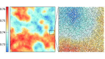
Figure 2: (Color online.) Passive system with $\phi=0.74$ in equilibrium. Left: the density plot constructed by averaging the local density over a region with radius equal to $20\,\sigma$ (similar results are obtained averaging over a region with radius in $[10,50]$). Right: a zoom over the region within the black square in the left plot showing the individual dumbbells close to the interface between a region with hexatic order (lower right) and a disordered sector (upper left). The color code is the same as in the left panel. The local hexatic map for this configuration is shown in the central upper panel in Fig. 3.

We start by studying the passive system. We use three kinds of initial states: random configurations with positions and orientations uniformly distributed, striped states with an ordered close-packed slab, and a hexatic-ordered state (see Sec. S1 in the SM). In all cases we present data evolved for sufficiently long to ensure that the initial state is forgotten and equilibration is reached. In the SM we exemplify the transient.

For $\phi<0.730$ any initial state with phase separation quickly melts and eventually evolves as a liquid. This is confirmed by the fact that translational and hexatic correlation functions decay exponentially with distance. Above $\phi\approx 0.756$ initial states with hexatic order remain ordered and the correlations decay very slowly (see Fig. S3). In between there is a regime with co-existence, as we now prove.

The first evidence for co-existence is given in Fig. 2 where we show the local density plot in equilibrium, with a zoom close to an interface between dense and sparse regions. The hexatic order in the region with high density and the lack of orientational order in the sparse region are clear in the zoom.

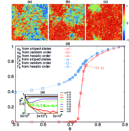
Figure 3: (Color online.) Passive system. (a-c) The local hexatic parameter, $\psi_{6j}$, in equilibrium configurations at $\phi=0.734\leavevmode\nobreak\ {\color[rgb]{0,0,0}\textrm{(a)}},\ 0.740\leavevmode\nobreak\ {\color[rgb]{0,0,0}\textrm{(b)}},\ 0.750\leavevmode\nobreak\ {\color[rgb]{0,0,0}\textrm{(c)}}$. (d) $\psi_{6}$ and $\Gamma_{6}$ defined in Eqs. (3) as functions of $\phi$. (e) Time evolution of $\psi_{6}$ from striped initial conditions at various densities with different solid lines. We also display the evolution at $\phi=0.74$ from random and hexatic-ordered initial states with dashed and dotted lines.

Further evidence for co-existence at this and other global densities is given in Fig. 3(a-c) where we show the local hexatic parameter on three equilibrium snapshots at $\phi=0.734,\ 0.740,\ 0.750$. These configurations are chosen at the long-time limit of the evolution of random initial states. The regions with local hexatic order are also regions of local high density and, conversely, in the sparse regions the dumbbells do not have orientational order (see Fig. S4 in the SM where the corresponding density plots as the one in Fig. 2 and histograms of the local densities are shown). In Fig. 3(d) we display the asymptotic $\psi_{6}$ and $\Gamma_{6}$ defined in Eq. (3) against $\phi$ for the three kinds of initial conditions. The data have been averaged over the last ten configurations (sampled every $\sim\,10^{4}$). The results confirm that the departing state is forgotten as the curves coincide within numerical accuracy. The $\psi_{6}$ curve for random initial configurations at $\phi\gtrsim 0.780$ is an exception and it still has to undergo a coarsening process to orient the clusters in the same direction, see Fig. S7 in the SM. All curves increase with $\phi$ indicating that the proportion of regions with hexatic order with respect to the disordered ones grows with $\phi$. The curve $\Gamma_{6}$ against $\phi$ is continuous and smooth while the one for $\psi_{6}$ although also continuous, shows a very steep increase starting at the smallest density at which co-existence appears. In Fig. 3(e) we show the time-dependence of $\psi_{6}$. The asymptote vanishes for $\phi<0.730$ but grows with $\phi$ for $\phi>0.730$. For $\phi=0.740$ we follow the evolution of different kinds of initial states to prove that they all approach the same asymptote. The evolution of the local $\psi_{6j}$ for these three initial conditions is illustrated in Fig. S2. The last one is at a time at which the (green) curves in Fig. 3 have reached the plateau. Additional signatures of liquid, coexisting and ordered phases are given in Fig. S5 that shows the structure factor for six $\phi$s.

Turning these arguments into a quantitative analysis, we find co-existence in the passive system in the interval $\phi\in[0.730,\ 0.756]$, approximately, justifying the extent of the grey region on the Pe = 0 axis in Fig. 1.

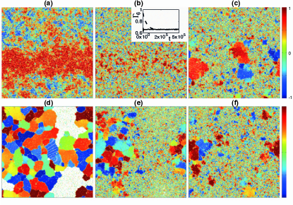
Figure 4: (Color online.) Time evolution at Pe = 10 and $\phi=0.734$. The initial states for the sequences (a-c) and (d-f) correspond to (a) a phase separated configuration at Pe = 0 evolved from a configuration with a striped-state of dumbbells and (d) the steady state at Pe = 40. The system is in its gas phase in the white zones (cfr. Fig. S12 (d) in the SM). The times at which the subsequent snapshots are taken are $t=2.5\times 10^{2}\leavevmode\nobreak\ \textrm{(b)},\,8.6\times 10^{5}\leavevmode\nobreak\ \textrm{(c)}$ and $t\,=\,10^{5}\leavevmode\nobreak\ \textrm{(e)},\,6\times 10^{5}\leavevmode\nobreak\ \textrm{(f)}$. As an inset in (b) we include the time-dependence of $\Gamma_{6}$ for the two runs.

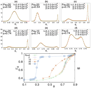
Figure 5: (Color online.) (a-f) Distributions of local densities at $\phi=0.52\leavevmode\nobreak\ {\color[rgb]{0,0,0}\textrm{(a)}},\ 0.54\leavevmode\nobreak\ {\color[rgb]{0,0,0}\textrm{(b)}},\ 0.7\leavevmode\nobreak\ {\color[rgb]{0,0,0}\textrm{(c)}}$ and fixed Pe$=20$ (first row, random initial configurations), and Pe $=20\leavevmode\nobreak\ {\color[rgb]{0,0,0}\textrm{(d)}},\ 10\leavevmode\nobreak\ {\color[rgb]{0,0,0}\textrm{(e)}},\ 0\leavevmode\nobreak\ {\color[rgb]{0,0,0}\textrm{(f)}}$ and $\phi=0.74$ (second row, starting from equilibrium configurations of the passive system). The various curves correspond to data sampled over different time intervals given in the keys. (g) $\Gamma_{6}$ as a function of $\phi$ for several Pe.

We now switch on activity. We first focus on $\phi=0.734$, a density within the interval of co-existence in the passive limit. In Fig. 4 we display the local hexatic order parameter of three instantaneous configurations obtained from the evolution at Pe = 10. The snapshots above are for an initial configuration with co-existence between a dense region with a rough horizontal form and a sparse region around it. Below are the snapshots for an initial stationary state at Pe = 40 where the system is strongly segregated. In the first case the system breaks the horizontal dense region and it later recreates dense clusters of approximately round form. These clusters turn independently of one another and have different (time-dependent) local hexatic order. Movie M1 illustrates the aforementioned dynamics at $\phi=0.74$, with more details on the cluster formation. In the second case, dumbbells are progressively evaporated from the large and dense clusters until less packed and smaller ones attain a stable size. Simultaneously, the regions in between the dense clusters reach the target density of the sparse phase. The subsequent dynamics are the same as for the steady state reached in the upper series of snapshots. In the inset we show the time-dependence of $\Gamma_{6}$ and we verify that the two runs reach the same asymptote. Therefore, independently of the initial conditions, the dynamics at $\phi=0.734$ and Pe = 10 approach a stationary limit with co-existence. The same occurs for all Pe at this $\phi$, even the very small ones (supplementary information on the Pe = 2 case is given in Fig. S8).

Having established that a small amount of activity does not destroy co-existence, we determine how it affects its limits by sweeping the parameters $\phi$ and Pe.

With the data for the coarse-grained local density at different pairs $(\phi,\ \mbox{Pe})$ we built the density distributions of Fig. 5(a-f). In the first row Pe = 20 and $\phi=0.52,\ 0.54,\ 0.7$ (Fig. S9 shows the dynamics at $\phi=0.54$). Figure 5(a) presents a static symmetric distribution around the global packing fraction that is in the liquid phase close to the boundary. Figure 5(b) shows the emergence of a second peak at a higher density, $\phi_{j}\simeq 0.9$, while the weight on lower density has displaced to a lower value of $\phi_{j}$. Figure 5(c) confirms the presence of the peak at $\phi_{j}\simeq 0.9$, the height of which has notably increased. Consequently, the weight on smaller local densities decreased and moved towards a slightly smaller value. The appearance of the second peak is our criterium to draw the upper boundary of the homogeneous phase, also complemented by the analysis of the structure factor in Fig. S11. At higher packing fractions the position of the second peak does not vary but its height increases at the expense of the one of the first peak. The upper boundary of the phase segregated region is naturally determined by the disappearance of the low density peak (configurations below and above the upper co-existence boundary are shown in Fig. S10).

The second row in Fig. 5 displays the Pe-dependence of the local density plots at $\phi=0.74$, inside the co-existence interval at Pe = 0. This analysis confirms continuity between the steady states in the passive and active cases, see also Fig. S14. The position of the high density peak moves towards larger $\phi_{j}$ for increasing Pe, indicating that the dense regions compactify, and accordingly the loose regions get more void. This fact reveals that segregation is more effective at higher Pe. Continuity upon increasing activity was also observed by analyzing the position of the density peaks moving along lines corresponding to equal proportions of disordered and hexatic regions in the system, see Figs. S13 and S15.

The hexatic order can also be used to analyze the phase diagram. At Pe = 0 we used the steep increase of $\psi_{6}$ (around $\phi=0.734$, see Fig. 3) to locate the boundary between liquid to phase separated phases since this quantity does not fluctuate much around its sample average. At finite Pe, instead, clusters with rather different values of $\psi_{6}$ co-exist and it is more convenient to use $\Gamma_{6}$ to study this boundary. In Fig. 5(g) we show $\Gamma_{6}$ as a function of $\phi$ for various Pe values. There is little dependence on Pe for, say, Pe $\lesssim 10$, while for larger values the shoulder moves towards smaller densities, signaling that the phase boundary becomes one between gas (very low $\phi$) and segregated phases at higher Pe.

An analysis of the statistics of the bead displacements at different time-delays and $(\phi,$ Pe) is given in Figs. S16 and S17 where, in particular, we distinguish the dynamics of the liquid and segregated dumbbells, for more details see the SM. Movies M2-M4 complement this survey with emphasis on coarsening at Pe = 2, 10, 20.

Putting these results together we drew the phase diagram in Fig. 1. The figure also includes some configurations at parameter values close to the limits of co-existence that clearly show liquid, phase separated and hexatic order. The lower boundary of the co-existence region decreases with increasing Pe since large activity favors the formation of high density clusters and therefore co-existence. Furthermore, co-existence is allowed at higher global packing fractions. This is because the regions with hexatic order become denser and leave more free space for the liquid phase under higher Pe . We conclude that we do not see any discontinuity between the behaviour of the system at Pe = 0 and Pe $>$ 0 at the densities at which there is phase co-existence in the passive limit.

As in a conventional liquid-vapor transition, it is hard to establish where the first-order transition lies with high precision. It would be desirable to complement our analysis with a thermodynamic study of the phase transitions. The double transition scenario proposed in Bernard and Krauth (2011) for the $2d$ passive hard disk problem was confirmed by the finite-size analysis of the equation of state, or packing-fraction dependence of the pressure in the NVT ensemble Bernard and Krauth (2011); Engel et al. (2013). In contrast, the existence of an equation of state in generic active matter remains open. Indeed, the difficulty to precisely define a pressure with the properties of a state variable in active systems was underlined in a number of papers, see e.g. Solon et al. (2015a); *solon2015pressure; Joyeux and Bertin (2016); Patch et al. (2016). The results here presented should further stimulate the search for a consistent definition of pressure for (molecular) active matter and promote new studies of phase diagrams in other active systems.