Space-Efficient Hidden Surface Removal

Abstract

We propose a space-efficient algorithm for hidden surface removal that combines one of the fastest previous algorithms for that problem with techniques based on bit manipulation. Such techniques had been successfully used in other settings, for example to reduce working space for several graph algorithms. However, bit manipulation is not usually employed in geometric algorithms because the standard model of computation (the real RAM) does not support it. For this reason, we first revisit our model of computation to have a reasonable theoretical framework. Under this framework we show how the use of a bit representation for the union of triangles, in combination with rank-select data structures, allows us to implicitly compute the union of $n$ triangles with roughly $O(1)$ bits per union boundary vertex. This results in an algorithm that uses at most as much space as the previous one, and depending on the input, can give a reduction of up to a factor $\Theta(\log n)$, while maintaining the running time.

1 Introduction

The search for algorithms that use as little storage as possible has received considerable attention in the last few years. This is due in part to the increase in data volumes that currently need to be processed and analyzed, and also to the widespread use of devices that have limited memory, ranging from embedded systems to mobile phones.

The first papers on space-efficient algorithms considered sorting [7, 33] as well as selection [17, 19, 32, 35]. More recently, space-efficient algorithms began to be studied for geometric and graph problems. The geometric problems studied include Delaunay triangulations and Voronoi diagrams [4, 29], linear programming and convex hulls [12, 15], visibility polygons [5], line segment intersections [27], and problems that can be solved by stack-based incremental algorithms (such as the construction of visibility polygons or polygon triangulations), among a few others [2, 4, 6]. For a recent survey, we refer to Korman [28].

The space-efficient algorithms for graph problems studied cover fundamental problems such as depth-first search, breadth-first search, computation of (strongly) connected components, cutvertices and shortest paths [3, 16, 24].

The setting where space-efficient algorithms are studied usually consists of a read-only input, a read-write working memory, and a write-only output memory. The general objective is to use as little working memory as possible. However, the actual goals and techniques used for space-efficient algorithms in computational geometry and graph algorithms are different, mostly due to the different computation models assumed. In computational geometry, the use of the real RAM puts the focus on algorithms that use as few variables as possible. In contrast, for space-efficient graph algorithms the model is often some variant of the word RAM, and the goal is to minimize the size of the working memory. To get a space bound that is independent from the size of a word, the space consumption of those algorithms is expediently measured in bits. The use of bits in the representation of words allows us to use a powerful set of existing algorithms and data structures that work on bit representations, such as rank-select data structures for bit vectors [14] and choice dictionaries for sets [23].

1.1 Computation model

A large body of research in computational geometry focuses on the analysis of the space and time requirements of algorithms that work on a real RAM. The time complexity is measured in the total number of fundamental operations on real numbers or integers, and the space complexity is the total number of memory cells used. In contrast, algorithms in other areas, such as graph algorithms, are often presented for variants of the word RAM, in which space is measured in bits. In this paper we are interested in applying some of the techniques used successfully for graph algorithms to geometric problems, but at the same time, we want to keep the conceptual transparency of the real RAM. We next briefly review these models.

Real RAM.

A real random access machine [9, 34] models an idealized computer that can manipulate arbitrary real numbers, and is the standard model of computation in computational geometry. The model represents data as an infinite sequence of storage cells. These cells can be of two different types: cells that can store real numbers, or cells that can store integers. The model supports standard operations on real numbers in constant time, including addition, multiplication, and elementary analytic functions such as taking roots, logarithms, trigonometric functions, etc. The model also supports standard arithmetic operations on integers, and in addition, integers can be used to directly address memory cells. In a sense, the model is a combination of a standard RAM (which we get by not using the real numbers), and a real-valued pointer machine [26] (which we get by never manipulating the integers).

The true power of the real RAM lies in the combination of the two data types. However, care must be taken: if we allow to freely convert real numbers to integers and vice versa, or indeed, if we can work with arbitrarily large integers at all, the model becomes unreasonably powerful and can solve PSPACE-complete problems in polynomial time [37]. The literature is inconsistent in dealing with this issue, but often a restricted floor function is (implicitly) assumed, that can convert, for instance, real numbers to their nearest integers in constant time only if the resulting integer is of polynomial size w.r.t. the input.

Word RAM.

A word RAM is similar to a real RAM without support for real numbers and with a limited number of bits available to encode integers. The word RAM represents data as a sequence of $w$-bit words, where it is usually assumed that $w=\Omega(\log n)$ where $n$ is the problem size. Integers on a real RAM are usually treated as atomic, whereas the word RAM allows for powerful bit-manipulation tricks. Data can be accessed arbitrarily, and standard operations, such as Boolean operations (and, xor, shl, $\ldots$), addition, or multiplication take constant time. One often assumes that the input is read-only, there is read and write access to the working-space, and the output is write-only. Then, the space-consumption of an algorithm is measured in the size of the required working-space.

There are many variants of the word RAM, depending on precisely which instructions are supported in constant time. The general consensus seems to be that any function in $\text{AC}^{0}$ is acceptable. However, it is always preferable to rely on a set of operations as small, and as non-exotic, as possible. Note that multiplication is not in $\text{AC}^{0}$ [21]. Nevertheless, it is usually included in the word RAM instruction set [20].

Bit manipulation in geometric algorithms.

While the majority of geometric algorithms are analyzed on a pure real RAM, the advantage of bit manipulation and the fact that the word RAM more closely resembles real-life computers, has led to several researchers mixing the two models and treating the integers in a real RAM as words [11, 30, 38]. When the model is handled carefully, this can lead to results that can run on a real world computer within the same resource bounds and that are hard or impossible to obtain on a pure real RAM.

However, these works only analyze the improved time complexity of such algorithms. The space complexity is harder to grasp—memory cells on a real RAM can store arbitrary numbers, while memory cells on a word RAM are restricted by their bits. The standard way to deal with this is to simply count all memory cells equal—when using floating point arithmetic to approximate real numbers in real-life computers, this is not an unreasonable assumption. However, when the majority of memory cells used in an algorithm store integers, rather than real numbers, we may in principle be able to significantly improve the space complexity through bit manipulation.

Model of choice.

In this paper, we will adopt a real RAM with words for integers in the most pure sense. That is:

• real numbers are stored and manipulated in real-valued memory cells, as on a real RAM;

• integer and bits are stored and manipulated integer-valued memory cells, as on a word RAM;

• absolutely no conversion between the two kinds of cells is allowed and only integers can be used to address memory cells.

As it is often the case for algorithms on the word RAM, we assume that the input is read-only and the output is write-only. In addition, we meassure the space consumption of our algorithms by the size of the required working space. Combining the word RAM and the real RAM is not new [10, 13]; however, most existing models are not restrictive enough concerning the conversion between the two kinds of cells, and one can exploit it to obtain algorithms that using an unrealistic amount of working space compared to what is possible on a real computer.

We apply these techniques to one concrete geometric problem: the computation of visibility from one observer among a set of polyhedral obstacles. This problem is closely related to hidden surface removal, a well-studied problem in computer graphics and computational geometry. More precisely, we present a space-efficient algorithm for computing the viewshed of a point in a three-dimensional scene. We give a space-efficient implementation of Katz et al.’s algorithm [25] that computes the viewshed from a point in a three-dimensional scene composed of $n$ triangles. The working space used by our algorithm consists of $O((U(n)+K)\log n)$ bits and $O(1)$ real numbers, where $K$ is a parameter that depends on the input, related to the complexity of unions of the input objects (a precise definition is given in Section 3). In the worst case, $K$ can be $\Theta(U(n)\log n)$ and our new algorithm matches the working space used by Katz et al.’s algorithm. However, we expect that in most practical situations, $K$ is closer to $\Theta(U(n))$, resulting in an improvement of a logarithmic factor.

Our main contribution is a concise representation of the union of triangles, together with a set of operations to manipulate them efficiently, which allows us to store intermediate results of the algorithm more efficiently. We choose Katz et al.’s algorithm for two reasons. Firstly, it is one of the fastest algorithms known for several types of scenes, including polyhedral terrains. This is relevant due to the many applications of this problem in geographic information systems. Secondly, it is a conceptually simple algorithm, making it appropriate to try to apply our bit-based techniques. Moreover, our technique works particularly well in the Katz et al. algorithm, because intermediate results are significantly larger than the final output. We expect that the same approach is applicable to more geometric problems.

We finally want to remark that there is a trivial algorithm to compute the viewshed of a point that runs $O(n\ell)$ time and uses $O(\log(n+\ell))$ bits where $n$ is the number of given polyhedral obstacles and $\ell$ denotes the total number vertices obtained by intersecting all pairs of obstacles: Iterate over all pairs and test if it is hidden by one obstacle. The viewshed consists of all boundaries of a polyhedral obstacle that connects 2 not-hidden vertices.

1.2 Hidden surface removal

Given a set of objects in 3D and a viewing point $p$, a fundamental question is to determine which parts of the objects are visible from $p$. This is sometimes called the viewshed of $p$. Equivalently, one may be interested in determining the parts not visible from $p$, which leads to the hidden surface removal problem.

Visibility problems of this type have been studied in computational geometry for a long time, due to the large number of applications that they have in computer graphics and geographic information systems (where the scene usually consists of a polyhedral terrain).

It is well-known that in a scene with complexity $\Theta(n)$ (e.g., consisting of $n$ triangles), the viewshed of a viewpoint can have $\Theta(n^{2})$ complexity, and can be computed in $O(n^{2})$ time [31]. Most practical algorithms are those that are output-sensitive: their running time is proportional to the complexity of the viewshed, $k$. The best running time for the most general case is achieved by the algorithm by Agarwal and Matousek [1], although at the expense of a fairly complicated method. Simpler but still efficient algorithms are known under the assumptions that a depth order among the 3D objects exists and can be computed efficiently (this is often, but not always, the case). For example, the algorithm by Goodrich [22] runs in $O(n\log n+\ell+t)$ time, where $\ell$ is the number of intersecting pairs of line segments, and $t$ the number of intersections between scene polygons, in the projection plane (note that in our context, all polygons are triangles, thus $t=O(s)$). The fastest algorithms under the depth-order assumption are the ones by Reif and Sen [36] and Katz et al. [25]. The former runs in time $O((n+k)\log n\log\log n)$, while the second one has running time $O((U(n)+k)\log^{2}n)$ and uses $O(U(n)\log n)$ integer/real numbers, where $U(n^{\prime})$ is a super-additive upper bound on the combinatorial complexity of the union of the projections of any $n^{\prime}$ objects from the input ($U(n)$ is nearly-linear for many classes of objects, such as polyhedral terrains).

1.3 Previous space-efficient algorithms

As already mentioned, the first problems studied in the setting of space-efficient algorithms were sorting [7, 33] and selection [17, 19, 32, 35]. Several researchers also considered space-efficient algorithms for geometric problems. Asano et al. [4] showed how to triangulate a planar point set and how to find a Delaunay triangulation or a Voronoi diagram in $O(n^{2})$ time with $O(\log n)$ bits working space where $n$ denotes the number of given points. Chan and Chen [12] presented a randomized algorithm for linear programming that, given an array of $n$ half-spaces in a constant number of dimensions, computes the lowest point in their intersection in $O(n)$ expected time and works with $O((\log n)^{2})$ bits. In addition, they described a randomized algorithm for computing the convex hull of $n$ points sorted from left to right in the plane (i.e., in two dimensions) that works with $O(n^{\epsilon})$ bits and runs in $O(n/\epsilon)$ expected time for any fixed $\epsilon>0$.

Later, several papers with time-space trade-offs were published. Darwish and Elmasry [15] solved the convex-hull problem to optimality with an algorithm that works with $\Theta(s)$ bits ($s\geq\log n$) and runs in $O(n^{2}/s+n\log s)$ time. An algorithm for computing a convex hull of a simple polygon was presented by Barba et al. [6]. They developed a general framework that can be applied to incremental linear-time algorithms that, given $n$ objects, use a stack of size $O(n)$ and possibly $O(1)$ further variables. The framework allows to reduce the space consumption of the algorithm to either $O(s)$ variables ($1\leq s\leq\log n$) at the price of an increased running time of $O(n^{2}\log n/2^{s})$ or to $O(p\log n/\log p)$ variables for any $2\leq p\leq n$ and time $O(n^{1+1/\log p})$. The framework can be used for computing the convex hull of a simple polygon as well as a triangulation of a monotone polygon, the shortest path between two given points inside a monotone polygon, and the visibility profile of a point inside a simple polygon. Moreover, the planar convex-hull problem has been solved optimally with an algorithm that runs in $O(n^{2}/s+n\lg s)$ time [15]. Konagaya and Asano gave an algorithm for reporting the line-segments intersections that runs in $O((n^{2}/\sqrt{s})\cdot\sqrt{\lg n}+n\lg s+k)$ time [27], where $k$ is the number of intersecting pairs. Other papers that deal with space-efficient geometric algorithms include [2, 4, 6]. Recently, Korman et al. [29] gave space-efficient algorithms for triangulations and for constructing Voronoi diagrams.

Furthermore, Barba et al. [5] described an algorithm for computing the visibility of a simple polygon with $n$ vertices that works with only $O(1)$ variables (which can store integers or real numbers) and has a running time of $O(nr)=O(n^{2})$ where $r$ is the number of the so-called reflex vertices of the polygon that are part of the output, and Elmastry and Kammer [18] focused on space-efficient plane-sweep algorithms.

Elmasry et al. [16] presented several basic graph algorithms: They showed that a depth-first search (DFS) can be carried out in $O((n+m)\log n)$ time with $((\log_{2}\!3)+\epsilon)n$ bits for arbitrary fixed $\epsilon>0$. A very similar result was found independently by Asano et al. [3], who need $cn$ bits for an unspecified constant $c>2$, or $\Theta(mn)$ time. Moreover, Elmasry et al. relaxed the space bound to $O(n)$ bits at the price of an increased running time of $O((n+m)\log\log n)$. In addition, they showed how to run a DFS in reverse with only a modest penalty of $O(n\log\log n)$ additional bits. Consequently, topological sortings and strongly connected components can be computed in linear time with $O(n\log\log n)$ bits. Although the connected components of a given undirected graph are usually computed by means of DFS, they observed that this bottleneck can be avoided and showed how to output the connected components in $O(n+m)$ time with $O(n)$ bits and how to compute a shortest path forest—and thus some variant of a breadth-first search (BFS)—within the same resource bounds.

1.4 Problem statement

The input to our problem is a set $D$ of $n$ triangles in $\mathbb{R}^{3}$, and a viewpoint $p$. The input is given as a list of triples of points, where each point is in turn given as a triple of real numbers. We assume that there exists a compatible depth order on the triangles, as seen from $p$, and we assume that the triangles are sorted in this order or that this order is computable in negligible time and space. Without loss of generality, we also assume that $n$ is a power of 2; otherwise, add $\leq n$ triangles inside one triangle. These new triangles do not modify the solution. We finally assume there are no three lines each extending a triangle edge that intersect in one point.

The output is a subdivision of each triangle into a visible and an invisible portion, where a point $q$ on a triangle is visible if the segment $pq$ does not intersect any other triangle of $D$. These visible portions are given as a list of polygons (possibly with holes). We denote their total complexity (that is, the total number of vertices of all these polygons together) by $k$.

2 Hidden surface removal algorithm by Katz et al.

We begin by describing the basic idea of the algorithm by Katz et al. [25]. The input triangles are stored in the leaves of a binary search tree $T$ in the given sorted order, with the nearest triangle in the rightmost leave. Each internal node $w\in T$ stores (1) the union $U_{w}$ of the projections of the triangles in the subtree rooted at $w$ as well as (2) the visible portions $V_{w}$ of $U_{w}$ (i.e., visible with respect to all input triangles). Note that $U_{w}$ and $V_{w}$ are planar regions that may contain holes. See Fig. 1 for an example of the partial unions $U_{i}$.

The main task of the algorithm is to compute $V_{w}$ for all leaves $w$ since then gluing together all visible parts of triangles results in the output. To accomplish this, the algorithm first builds the partial unions $U_{i}$ in a bottom-up fashion, by computing, at each internal node, the union of the unions stored in both subtrees. Once $U_{root}$ is built, the visible portions are produced by traversing $T$ recursively in preorder. At any time during the algorithm, only the visibility regions along one path are stored. It follows that the space bottleneck of the algorithms comes from storing the $U_{i}$ in each of the nodes, that are required for the whole tree, adding up to $O(U(n)\log n)$ integer/real numbers.

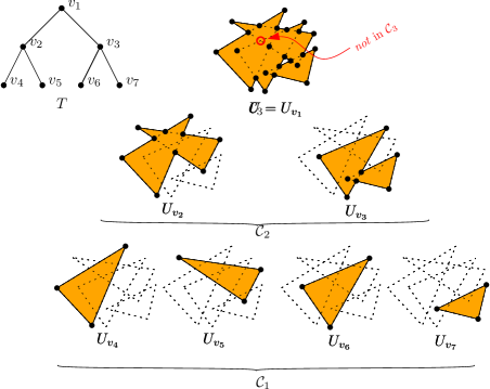
Figure 1: Partial unions $U_{i}$ associated to a tree $T$ for four triangles.

3 Space-efficient union representation

We present a method to build the tree of partial unions $U_{i}$ following the same recursive procedure as in [25]. The main difference will be in how each union is represented and stored.

The idea behind our method will be best illustrated with a running example. Consider the example in Fig. 3, showing the same four triangles as in Fig. 1. The vertices of the union of $n$ triangles are a subset of those in their overlay (i.e., all pairwise edge intersections), or equivalently, vertices from the union of subsets of them. However, as shown in the figure, not all of these vertices will show up in the union of the whole set.

The parameter $K$ is defined as the sum of the complexities of the partial unions $U_{i}$ over all levels of the tree. $K$ is $O(U(n)\log n)$ since the tree has height $O(\log n)$ and each level of the tree corresponds to an instance of size $n$ with complexity $U(n)$. This bound is tight since there are constructions for which $K=\Theta(U(n)\log n)$ as shown in Figure 3. However, we point out that this situation occurs due to a combination of the actual geometry of the triangles with the way in which triangles have been grouped in the tree of partial unions. In practical situations, we expect such constructions to be uncommon.

Our method represents partial unions by using bit vectors, so that each boundary vertex of a partial union is encoded with $O(1)$ bits, instead of with $O(1)$ numbers. Moreover, our algorithm processes the nodes of the tree with increasing heights of the nodes, starting from the leaves. We say that the nodes in the tree are processed level by level, where level 1 consists of the leaves of the tree, level 2 is made of the parents of the leaves, and so on, until the root in level $\ell=\lceil\log_{2}n\rceil+1$.

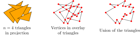
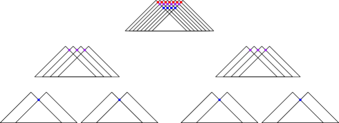
Figure 2: An example instance.

Figure 3: Example with 8 triangles and a tree of partial unions such that in each node many union vertices appear. Generalizing the construction to $n$ triangles results in $K=\Theta(U(n)\log n)$, which is worst possible.

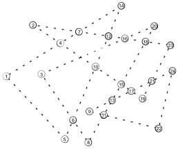
Figure 4: Detail of triangles in Fig. 3 showing vertex numbers for the vertices involved in the computation in Fig. 1.

The three main ingredients of our representation will be a vector ${\mathcal{C}}_{i}$, a set of bit vectors associated with ${\mathcal{C}}_{i}$, denoted $B_{i,j}$, and a set of triangle bit vectors $A_{w}$. For $i\in\{1,\ldots,\ell\}$, let ${\mathcal{C}}_{i}$ be an array with all vertices that potentially can appear in $U_{w}$ for all nodes $w$ in levels $1,\dots,i$, see Fig. 4. It will be important to store ${\mathcal{C}}_{i}$ in a special way and to store some extra information. Note that ${\mathcal{C}}_{i}$ and its extra info will be stored only once and used for all nodes of the tree that are in levels $1,\ldots,i$.

We assume that the triangles are numbered from $1$ to $n$. ${\mathcal{C}}_{i}$ is stored in an array $C_{i}[1,\ldots,n]$ where each entry $C_{i}[k]$ is an array itself that stores the vertices that are on the boundary of the $j$th triangle and that are used by some $U_{w}$ for a node $w$ in some level $1\dots i$. Moreover, the vertices in $C_{i}[k]$ are stored in the order found when walking along the boundary of a triangle $\triangle$ in clockwise direction. Note that some vertices are the intersection of the boundaries of two triangles $k^{\prime}$ and $k^{\prime\prime}$, and thus they are stored in both arrays $C_{i}[k^{\prime}]$ and $C_{i}[k^{\prime\prime}]$. We also store cross pointers between these two entries—a concept introduced for undirected graphs [16]. For each triangle $k$, we also store the number $p_{i}$ of vertices in $C_{i}[k]$ as well as the prefix sums $P_{x}=\sum_{y=1}^{x}p_{y}$.

All the arrays $C_{i}[1],C_{i}[2],C_{i}[3],\ldots$ are stored in consecutive order and we consider it as a global array, which we identify with the name ${\mathcal{C}}_{i}$. Thus, each vertex in the set ${\mathcal{C}}_{i}$ has an absolute position $p\in\{1,\ldots,|{\mathcal{C}}_{i}|\}$ in the array ${\mathcal{C}}_{i}$. Using the prefix sums we can translate between the $j$th vertex of the $k$th triangle and its absolute position $p$ in ${\mathcal{C}}_{i}$. See Table 1 for the vectors that correspond to our example.

${{\mathcal{C}}_{1}}$	: 1,14, 5| 2,23,19| 3,20, 8| 9,24,22
${B_{1,1}}\!\!$	: 1, 1, 1| 1, 1, 1| 1, 1, 1| 1, 1, 1
${{\mathcal{C}}_{2}}$	: 1, 4, 7,14,12,10, 5| 2, 7,12,23,19,10, 4| 3,20,13,11, 8| 9,13,24,22,11
${B_{2,1}}\!\!$	: 1, 0, 0, 1, 0, 0, 1| 1, 0, 0, 1, 1, 0, 0| 1, 1, 0, 0, 1| 1, 0, 1, 1, 0
${B_{2,2}}\!\!$	: 1, 1, 1, 1, 1, 1, 1| 1, 1, 1, 1, 1, 1, 1| 1, 1, 1, 1, 1| 0, 1, 1, 1, 1
${{\mathcal{C}}_{3}}$	: 1, 4, 7,14,12,10, 6, 5| 2, 7,12,16,18,23,21,19,17,15,10, 4| 3,16,20,18,15,13,11, 8, 6| 9,13,17,21,24,22,11
${B_{3,1}}\!\!$	: 1, 0, 0, 1, 0, 0, 0, 1| 1, 0, 0, 0, 0, 1, 0, 1, 0, 0, 0, 0| 1, 0, 1, 0, 0, 0, 0, 1, 0| 1, 0, 0, 0, 1, 1, 0
${B_{3,2}}\!\!$	: 1, 1, 1, 1, 1, 1, 0, 1| 1, 1, 1, 0, 0, 1, 0, 1, 0, 0, 1, 1| 1, 0, 1, 0, 0, 1, 1, 1, 0| 0, 1, 0, 0, 1, 1, 1
${B_{3,3}}\!\!$	: 1, 1, 1, 1, 1, 0, 1, 1| 1, 1, 1, 1, 1, 1, 1, 0, 1, 1, 0, 1| 0, 1, 1, 1, 1, 1, 1, 1, 1| 0, 1, 1, 1, 1, 1, 1

Table 1: Vectors ${{\mathcal{C}}_{i}}$ and $B_{i,j}$ for our example.

Based on ${\mathcal{C}}_{i}$, we can define bit vectors $B_{i,j}$. For each level $j\leq i$, $B_{i,j}$ is a bit vector with the same size as ${\mathcal{C}}_{i}$, following the same triangle structure as ${\mathcal{C}}_{i}$: each group of consecutive entries represents one of the input triangles. $B_{i,j}$ is defined as follows: $B_{i,j}[k]=1$ exactly when the vertex ${\mathcal{C}}_{i}[k]$ appears in the partial union of level $j$ that includes the corresponding triangle. This means that $U_{w}$ and $U_{w^{\prime}}$ with $w\neq w^{\prime}$ are stored in the same bit vector $B_{i,j}$ whenever $w$ and $w^{\prime}$ are in the same level $j$. This is possible since the intersection points are pairwise disjoint in each level and thus each vertex is part of at most one set $U_{w}$ or $U_{w^{\prime}}$. We refer again to Table 1 for an example.

Finally, we store for each node $w$ a bit vector $A_{w}$ over the triangles that are identified with descendants of $w$ as follows: there is a $1$ for a triangle exactly when the boundary of the triangle is part of the boundary of $U_{w}$.

With these data structures in place, consider now the computation of $U_{w}$ for all nodes $w$ in level $i+1$, given the bit vectors $B_{i,j}$ over ${\mathcal{C}}_{i}$ for each level $j<i+1$. Assume for now that based on the bit vectors $B_{i,j}$ we can determine $U_{w^{\prime}}$ for all nodes $w^{\prime}$ in a level $j<i+1$ (we defer the details of this to the next section). Then we can compute $U_{w}$ for all nodes $w$ in level $i+1$. In particular, we can determine the set ${\mathcal{C}}_{i+1}$ as the union of ${\mathcal{C}}_{i}$ and the new vertices found on the boundary $U_{w}$ of some node $w$ in level $i+1$, which can be computed using the standard intersection algorithm by Bentley and Ottmann [8]. However, instead of storing intersection points using real-valued memory cells, we store them implicitly, by storing the indices of the two segments of the input that generate the intersection point. This allows us to store all necessary information for a vertex using $O(\log n)$ bits.

Note also that for each $U_{w}$ of the nodes $w$ in the tree, we store a pointer to a vertex in ${\mathcal{C}}_{i}$ that can be used as start vertex to traverse the boundary components of $U_{w}$. In our example, the pointer could point to the following vertices: $v_{1}:1,13$ (we store two pointers since $U_{v_{1}}$ has an outer boundary and a hole) $v_{2}:1$, $v_{3}:3$, $v_{4}:1$, $v_{5}:2$, $v_{6}:8$, $v_{7}:22$.

It is important to note that at any time during the algorithm, we only need to maintain $C_{i}$ and the $B_{i,j}$ vectors for the previous and current level.

3.1 Reconstructing lower-level unions with rank-select data structures

In order to determine $U_{w^{\prime}}$ for nodes $w^{\prime}$ in level $i+1$, we need to know $U_{w}$ for nodes $w$ in levels 1 to $i$. In this section we describe how to use the bit vector $B_{i,j}$ over ${\mathcal{C}}_{i}$ of level $j\leq i$ to reconstruct $U_{w}$ for a node $w$ in level $j$. The key ingredient is to build a rank-select data structure on each bit vector $B_{i,j}$ and each bit vector $A_{w}$.

Rank-select data structures.

A rank-select data structure for a bit sequence $B=(b_{1},\ldots,b_{N})$ is a data structure that supports two types of queries: $\mathrm{rank}_{B}(j)$ ($j\in\{1,\ldots,N\}$), which returns $\sum_{i=1}^{j}b_{i}$; and $\mathrm{select}_{B}(k)$ ($k\in\{1,\ldots,\sum_{i=1}^{N}b_{i}\}$), which returns the smallest $j\in\{1,\ldots,N\}$ with $\mathrm{rank}_{B}(j)=k$. It is well-known that rank-select structures for bit sequences of length $N$ that support rank and select queries in constant time and occupy $O(N)$ bits of space can be constructed in $O(N)$ time [14]. All rank-select data structures introduced below are of this type.

Computing $U_{w}$.

To compute a set $U_{w}$ for a node $w$ in level $j$, we proceed as follows: Color all triangles white (more precisely, always have a color array where all triangles are white, then use it, and at the end of the usage, undo the recoloring). Using the rank select structure over $A_{w}$ we determine a white triangle $k^{\prime}$ that has some common boundary with $U_{w}$, then we use the rank-select structure on $B_{i,j}$ to find a first vertex that is on the boundary of $U_{w}$ and of $k^{\prime}$, and can translate the absolute position of the vertex to a relative position in $C_{i}[k^{\prime}]$. We next start an iteration to find the rest of the closed curve around the boundary of $U_{w}$. We always know a vertex part of the boundary of a triangle $k^{\prime}$; and this vertex is either the corner of a triangle or an intersection point of $k^{\prime}$ with another triangle. Making use of the rank-select structures we can skip over the corners and assume without loss of generality that the current vertex is an intersection point of $k^{\prime}$ with another triangle $k^{\prime\prime}$. More exactly, we know the position of the vertex in $C_{i}[k^{\prime}]$ where we can follow a cross pointer to the position of the same vertex in $C_{i}[k^{\prime\prime}]$. Using the prefix sums we get the absolute position of the vertex in ${\mathcal{C}}_{i}$. The rank-select structure allows us to find the next vertex on the closed curve, which is w.l.o.g. a vertex of an intersection point between the triangle $k^{\prime\prime}$ and another triangle $k^{\prime\prime\prime}$. Following again a cross pointer we can now jump to that vertex in $C_{i}[k^{\prime\prime\prime}]$. Whenever we extend the boundary by some vertex, we test if all vertices of the current triangle are now part of the boundary (using a separate counter for each triangle). If so, we color the triangle black. After we have found a closed curve, if there are still white triangles in $A_{w}$, then the boundary of $U_{w}$ has holes, so we we rerun the procedure.

We illustrate this in our example by showing how to reconstruct $U_{v_{3}}$ using ${{\mathcal{C}}_{3}}$ and ${B_{3,2}}$. We start at vertex 3 in ${{\mathcal{C}}_{3}}$. Using the rank-select structures, we find the vertex after 3 that also has a 1 in ${B_{3,2}}$, which is vertex 20. Since 20 is a vertex of a triangle (20 has no cross pointer), we are looking for the next 1 in ${B_{3,2}}$, which is vertex 13. Then we use the cross pointer to jump to the other 13 in ${{\mathcal{C}}_{3}}$. Again, we are looking for the next 1s in ${B_{3,2}}$ and find so 24 and subsequently 22 in ${{\mathcal{C}}_{3}}$, which are both corners of a triangle. So we continue and find 11. Using again a cross pointer, we jump to the other 11 in ${{\mathcal{C}}_{3}}$, search for the next 1 in ${B_{3,2}}$ and find 8. Searching for the next one in ${B_{3,2}}$, we find 3 since we have to consider each part as cyclic. Since 3 is the vertex where we begun, we are done.

It remains to analyze the required working space. While processing the nodes in level $i$, we store vertex numbers in ${{\mathcal{C}}_{i^{*}}}$ and suitable cross pointers for levels $i^{*}\in\{i-1,i\}$. Since each vertex number and each cross pointer can be stored with $O(\log n)$ bits, and ${{\mathcal{C}}_{i^{*}}}$ cannot have more vertices that those that appear over the partial unions in the tree, ${{\mathcal{C}}_{i^{*}}}$ can be stored with $(O(U(n)+K)\log n)$ bits, for the whole tree. In addition, we have $O(\log n)$ bit vectors ${B_{i^{*},1}},\ldots,{B_{i^{*},i^{*}}}$ of $O(U(n)+K)$ bits each. In total, the algorithm uses $O((U(n)+K)\log n)$ bits.

Theorem 3.1

There is an algorithm that reports the union of a set of $n$ non-intersecting triangles in 3D in time $O((U(n)+k)\log^{2}n)$ by using $O((U(n)+K)\log n)$ bits of working space and $O(1)$ real numbers, where $U(n^{\prime})$ is a super-additive bound on the maximal complexity of the union of any $n’$ triangles from the family under consideration, $k$ is the complexity of the output, and $K$ is the sum of the complexities of the partial unions over all levels of the recursion tree used by the algorithm.

4 Application to the algorithm by Katz et al.

As mentioned before, the space bottleneck in the algorithm by Katz et al. is the storage of the partial unions $U_{w}$. Therefore we can directly apply our technique, replacing the representation of the partial union boundaries by our bit-based representation, automatically reducing the storage used in terms of bits.

The only detail remaining is how to store $V_{w}$. In contrast to the sets $U_{w}$, we do not have the property that the sets $V_{w}$ and $V_{w^{\prime}}$ of one level have disjoint vertices. Thus, we use one bit vector over $U$ for each such set. Concerning the space consumption this is no problem since we have to store such a bit vector only for the nodes that are part of a root-to-leaf path in the tree.

Theorem 4.1

Consider a set of $n$ non-intersecting triangles in space and a viewing point $p$, such that there exists a known depth ordering of the objects with respect to $p$, and such that the union of the projections of any $n^{\prime}$ of the objects on a viewing plane has complexity $U(n^{\prime})$, where $U(n^{\prime})$ is super-additive. Then the visibility map from $p$ can be reported with $O((U(n)+k)\log^{2}n)$ time, using $O((U(n)+K)\log n)$ bits of working space and $O(1)$ real numbers, where $k$ is the complexity of the visibility map, and $K$ is the sum of the complexities of the partial unions over all levels of the recursion tree used by the algorithm.

5 Conclusion

We have shown that techniques previously used for graph algorithms can also be applied to geometric problems. In line with recent results for graph algorithms [3, 16, 24], the space consumption to compute the viewshed of a point in a three-dimensional scene can be reduced by a factor of $\Theta(\log n)$ while maintaining the running time. However, the space used ultimately depends on the complexities of the intermediate unions along the recursion tree, represented by the parameter $K$, which sometimes can be $\Theta(U(n)\log n)$. It may be possible to reduce the dependency on the intermediate unions by storing only the union vertices in each level that contribute to the current union, and not the rest. Exploring this direction further is an interesting direction for further research.

References

- [1] Pankaj K. Agarwal and Jirí Matousek. Ray shooting and parametric search. SIAM J. Comput., 22(4):794–806, 1993.
- [2] Tetsuo Asano, Kevin Buchin, Maike Buchin, Matias Korman, Wolfgang Mulzer, Günter Rote, and André Schulz. Reprint of: Memory-constrained algorithms for simple polygons. Comput. Geom. Theory Appl., 47(3, Part B):469–479, 2014.
- [3] Tetsuo Asano, Taisuke Izumi, Masashi Kiyomi, Matsuo Konagaya, Hirotaka Ono, Yota Otachi, Pascal Schweitzer, Jun Tarui, and Ryuhei Uehara. Depth-first search using bits. In Proc. 25th International Symposium on Algorithms and Computation (ISAAC 2014), volume 8889 of LNCS, pages 553–564. Springer, 2014.
- [4] Tetsuo Asano, Wolfgang Mulzer, Günter Rote, and Yajun Wang. Constant-work-space algorithms for geometric problems. J. Comput. Geom., 2(1):46–68, 2011.
- [5] Luis Barba, Matias Korman, Stefan Langerman, and Rodrigo I. Silveira. Computing a visibility polygon using few variables. Comput. Geom. Theory Appl., 47(9):918–926, 2014.
- [6] Luis Barba, Matias Korman, Stefan Langerman, Rodrigo I. Silveira, and Kunihiko Sadakane. Space-time trade-offs for stack-based algorithms. In Proc. 30th International Symposium on Theoretical Aspects of Computer Science (STACS 2013), volume 20 of LIPIcs, pages 281–292. Schloss Dagstuhl – Leibniz-Zentrum für Informatik, 2013.
- [7] Paul Beame. A general sequential time-space tradeoff for finding unique elements. SIAM J. Comput., 20(2):270–277, 1991.
- [8] Jon Louis Bentley and Thomas Ottmann. Algorithms for reporting and counting geometric intersections. IEEE Trans. Computers, 28(9):643–647, 1979.
- [9] Lenore Blum, Mike Shub, and Steve Smale. On a theory of computation and complexity over the real numbers: NP-completeness, recursive functions and universal machines. Bull. Amer. Math. Soc. (N.S.), 21(1):1–46, 07 1989.
- [10] Vasco Brattka and Peter Hertling. Feasible real random access machines. J. Complexity, 14(4):490–526, 1998.
- [11] Karl Bringmann and Tobias Friedrich. Exact and efficient generation of geometric random variates and random graphs. In Proc. 40th International Colloquium on Automata, Languages, and Programming (ICALP 2013), Part I, pages 267–278, 2013.
- [12] Timothy M. Chan and Eric Y. Chen. Multi-pass geometric algorithms. Discrete Comput. Geom., 37(1):79–102, 2007.
- [13] Timothy M. Chan and Mihai Pǎtraşcu. Transdichotomous results in computational geometry. I. Point location in sublogarithmic time. SIAM J. Comput., 39(2):703–729, 2009.
- [14] David Clark. Compact Pat Trees. PhD thesis, University of Waterloo, Waterloo, Ontario, Canada, 1996.
- [15] Omar Darwish and Amr Elmasry. Optimal time-space tradeoff for the 2D convex-hull problem. In Proc. 22nd Annual European Symposium on Algorithms (ESA 2014), volume 8737 of LNCS, pages 284–295. Springer, 2014.
- [16] Amr Elmasry, Torben Hagerup, and Frank Kammer. Space-efficient basic graph algorithms. In Proc. 32nd International Symposium on Theoretical Aspects of Computer Science, (STACS 2015), volume 30 of LIPIcs, pages 288–301. Schloss Dagstuhl – Leibniz-Zentrum für Informatik, 2015.
- [17] Amr Elmasry, Daniel Dahl Juhl, Jyrki Katajainen, and Srinivasa Rao Satti. Selection from read-only memory with limited workspace. Theor. Comput. Sci., 554:64–73, 2014.
- [18] Amr Elmasry and Frank Kammer. Space-efficient plane-sweep algorithms. In Proc. 27th International Symposium on Algorithms and Computation (ISAAC 2016), volume 64 of LIPIcs, pages 30:1–30:13. Schloss Dagstuhl – Leibniz-Zentrum für Informatik, 2016.
- [19] Greg N. Frederickson. Upper bounds for time-space trade-offs in sorting and selection. J. Comput. Syst. Sci., 34(1):19–26, 1987.
- [20] Michael L. Fredman and Dan E. Willard. Trans-dichotomous algorithms for minimum spanning trees and shortest paths. J. Comput. System Sci., 48(3):533–551, 1994.
- [21] Merrick Furst, James B. Saxe, and Michael Sipser. Parity, circuits, and the polynomial-time hierarchy. Math. Systems Theory, 17(1):13–27, 1984.
- [22] Michael T. Goodrich. A polygonal approach to hidden-line and hidden-surface elimination. CVGIP: Graphical Model and Image Processing, 54(1):1–12, 1992.
- [23] Torben Hagerup and Frank Kammer. Succinct choice dictionaries. Computing Research Repository (CoRR), arXiv:1604.06058 [cs.DS], 2016.
- [24] Frank Kammer, Dieter Kratsch, and Moritz Laudahn. Space-Efficient Biconnected Components and Recognition of Outerplanar Graphs. In 41st International Symposium on Mathematical Foundations of Computer Science (MFCS 2016), volume 58 of LIPIcs, pages 56:1–56:14. Schloss Dagstuhl – Leibniz-Zentrum für Informatik, 2016.
- [25] Matthew J. Katz, Mark H. Overmars, and Micha Sharir. Efficient hidden surface removal for objects with small union size. Comput. Geom. Theory Appl., 2:223–234, 1992.
- [26] Donald Ervin Knuth. The Art of Computer Programming: Fundamental Algorithms, volume 1. Addison-Wesley, 3rd edition, 1997.
- [27] Matsuo Konagaya and Tetsuo Asano. Reporting all segment intersections using an arbitrary sized work space. IEICE TRANSACTIONS on Fundamentals of Electronics, Communications and Computer Sciences, 96-A(6):1066–1071, 2013.
- [28] Matias Korman. Memory-constrained algorithms. In Encyclopedia of Algorithms, pages 1260–1264. Springer, 2016.
- [29] Matias Korman, Wolfgang Mulzer, Andre van Renssen, Marcel Roeloffzen, Paul Seiferth, and Yannik Stein. Time-space trade-offs for triangulations and Voronoi diagrams. In Proc. 14th Algorithms and Data Structures Symposium (WADS 2015), 2015.
- [30] Drago Krznaric and Christos Levcopoulos. Computing a threaded quadtree from the Delaunay triangulation in linear time. Nordic J. Comput., 5(1):1–18, 1998.
- [31] Michael McKenna. Worst-case optimal hidden-surface removal. ACM Trans. Graph., 6(1):19–28, January 1987.
- [32] J. Ian Munro and Venkatesh Raman. Selection from read-only memory and sorting with minimum data movement. Theor. Comput. Sci., 165(2):311–323, 1996.
- [33] Jakob Pagter and Theis Rauhe. Optimal time-space trade-offs for sorting. In Proc. 39th Annual IEEE Symposium on Foundations of Computer Science (FOCS 1998), pages 264–268. IEEE Computer Society, 1998.
- [34] Franco P. Preparata and Michael I. Shamos. Computational Geometry: An Introduction. Springer, 1985.
- [35] Venkatesh Raman and Sarnath Ramnath. Improved upper bounds for time-space trade-offs for selection. Nord. J. Comput., 6(2):162–180, 1999.
- [36] John H. Reif and Sandeep Sen. An efficient output-sensitive hidden surface removal algorithm and its parallelization. In Proc. 4th Annu. ACM Sympos. Comput. Geom. (SoCG), pages 193–200. ACM, 1988.
- [37] Arnold Schönhage. On the power of random access machines. In Proc. 6th Internat. Colloq. Automata Lang. Program. (ICALP), pages 520–529, 1979.
- [38] Okke Schrijvers, Frits van Bommel, and Kevin Buchin. Delaunay triangulations on the word RAM: Towards a practical worst-case optimal algorithm. In Proc. 10th International Symposium on Voronoi Diagrams in Science and Engineering (ISVD 2013), pages 7–15. IEEE Computer Society, 2013.