A massive momentum-subtraction scheme

Abstract

A new renormalization scheme is defined for fermion bilinears in QCD at non vanishing quark masses. This new scheme, denoted RI/mSMOM, preserves the benefits of the nonexceptional momenta introduced in the RI/SMOM scheme, and allows a definition of renormalized composite fields away from the chiral limit. Some properties of the scheme are investigated by performing explicit one-loop computation in dimensional regularization.

I Introduction

Nonperturbative renormalization MOM schemes have been introduced in Refs. Martinelli:1994ty ; Sturm:2009kb by imposing a set of renormalization conditions, which specify the renormalization of the fermion wave function, of the fermion mass, and of composite operators like fermion bilinears. The renormalization conditions are imposed in the chiral limit of QCD, and therefore, by construction, these schemes are mass-independent, meaning that all the renormalization constants are independent of the value of the fermion mass. This is useful for instance when considering ratios of quantities such as masses; in a mass-independent scheme $m_{i}/m_{j}$ for two different fermions $i$ and $j$, does not renormalize since the renormalization constants cancel between the numerator and the denominator. The renormalization conditions are chosen so that renormalized correlators involving the vector and axial currents satisfy the Ward identities (WIs) dictated by the symmetries of the theory. Using massless schemes for massive quarks involves violations of the Ward identities by terms that scale like powers of $m/\mu$, where $\mu$ is the typical energy scale of the correlators that are computed.

Recent lattice studies have begun investigating the nonperturbative dynamics of heavy quarks like charm and bottom, including these heavy flavors as relativistic dynamical degrees of freedom in the path integral. In current simulations the mass of the heavy quarks is often of the same order of magnitude as the UV cutoff, defined as the inverse lattice spacing $a^{-1}$. As a consequence, it is not possible to reach a regime where there is a clear separation between the fermion mass, the renormalization scale, and the cutoff, i.e. a regime where $m\ll\mu\ll a^{-1}$. When studying heavy quarks, it may be interesting to introduce a massive scheme, i.e. a scheme where the renormalization conditions are imposed at some finite value of the renormalized mass. It is indeed possible to choose the renormalization conditions in such a way that the desirable properties of the massless schemes are preserved, in particular the Ward identities would hold exactly at finite values of the quark mass, and independently of the ratio $m/\mu$.

In this paper, we define a massive scheme for axial and vector currents as well as scalar and pseudoscalar densities, which we call mSMOM. The renormalization constants defined in mSMOM satisfy properties that are similar to the ones found in SMOM Sturm:2009kb . SMOM was introduced in order to reduce chiral symmetry breaking and other unwanted infrared effects, by defining the renormalization conditions for the vertex functions at a symmetric subtraction point which involves non-exceptional momenta. The key property of the SMOM scheme is that the renormalization conditions are defined so that the renormalized WIs are satisfied. This is in contrast with MOM where the WI for the axial current are recovered only for large values of $\mu^{2}$ Sturm:2009kb . Starting from SMOM, we modify some of the renormalization conditions in order to recover the massive renormalized WIs. The renormalization conditions for massive quarks require the introduction of an extra scale $\overline{m}$, which is the value of the renormalized mass at which the conditions are spelled out. As we take the limit $\overline{m}\to 0$, our scheme reduces to SMOM, so that we are able to interpolate between massive and massless schemes.

We discuss a number of properties using non-perturbative arguments after which we perform an explicit check at one-loop in perturbation theory using dimensional regularization. While the results of this calculation is exactly as expected, it is pleasing to see explicitly a number of nontrivial cancellations. We then focus on the case of the lattice currents, and discuss their renormalization in mSMOM. The massive schemes can be implemented numerically, in order to obtain nonperturbative determinations of the corresponding renormalization constants. The massive renormalization constants will change some lattice artefacts $O(a^{2}m^{2})$, and could potentially lead to smoother extrapolations to the continuum limit of phenomenologically relevant observables. A first qualitative understanding of the can be obtained by a perturbative study along the lines of Ref. Athenodorou:2011zp , but ultimately dedicated numerical studies are necessary in order to settle this issue.

II Massive renormalization conditions

A regularization independent momentum subtraction scheme for bilinears with a nonexceptional, symmetric point has been introduced in Ref. Sturm:2009kb , under the name of RI/SMOM. RI/SMOM is a mass-independent renormalization scheme, in that all the renormalization conditions are specified in the chiral limit, and therefore the renormalization constants cannot depend on the quark masses by definition. Before investigating the possibility of defining a similar scheme at finite quark mass, let us briefly recall the renormalization conditions that define RI/SMOM, and discuss the main properties of the renormalized bilinears in that scheme.

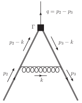
Figure 2: Diagram representing the non-amputated vertex function at 1-loop in perturbative QCD.

Fig. 2 summarises the kinematics used in this paper: the correlators of fermion bilinears with two external off-shell fermions are

$$G^{a}_{\Gamma}(p_{3},p_{2})=\langle O^{a}_{\Gamma}(q)\bar{\psi}(p_{3})\psi(p_{2})\rangle\,,$$ (1)

where $O^{a}_{\Gamma}=\bar{\psi}\Gamma\tau^{a}\psi$ is a flavor non-singlet fermion bilinear, and $\Gamma$ spans all the elements of the basis of the Clifford algebra, which we denote as $\Gamma=\mathrm{S},\mathrm{P},\mathrm{V},\mathrm{A},\mathrm{T}$. Note that $\tau^{a}$ denotes a generic generator of rotations in flavor space. The conventions for the Dirac gamma matrices are spelled out in detail in App. A. The four dimensional vectors $p_{2}$ and $p_{3}$ are respectively the incoming and outgoing momenta of the external fermions, and momentum conservation requires $q=p_{2}-p_{3}$. The kinematics adopted in this work is the one used in Ref. Sturm:2009kb :

$$p_{2}^{2}=p_{3}^{2}=q^{2}=-\mu^{2}\,.$$ (2)

Following the convention in the paper above, we denote this symmetric point by the shorthand “$\mathrm{sym}$”.

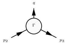
Figure 1: Kinematics used for the correlators of fermion bilinears.

For the purpose of illustration, we can consider the case of a fermion doublet

$$\psi=\begin{pmatrix}\psi_{1}\\ \psi_{2}\end{pmatrix}\,,~{}~{}\overline{\psi}=\begin{pmatrix}\overline{\psi}_{1}&\overline{\psi}_{2}\end{pmatrix},$$ (3)

with mass matrix

$$\mathcal{M}=\begin{pmatrix}m_{1}&0\\ 0&m_{2}\end{pmatrix}.$$ (4)

Note that in the mass degenerate case, we simply have $\mathcal{M}=m\mathds{1}$. If we choose $\tau^{a}=\tau^{+}=\frac{\sigma^{+}}{2}=\frac{1}{2}\left(\sigma^{1}+i\sigma^{2}\right)$, then the bilinear $O^{a}_{\Gamma}=\bar{\psi}\Gamma\tau^{a}\psi$ takes the form $O_{\Gamma}=\overline{\psi}_{1}\Gamma{\psi_{2}}$.

The infinitesimal vector and axial non-singlet SU(2) chiral transformation are as follows

$$\delta\psi(x)=i\Big{[}\alpha_{V}(x)\tau^{a}\Big{]}\psi(x)\,,~{}~{}\delta\overline{\psi}(x)=-i\overline{\psi}(x)\Big{[}\alpha_{V}(x)\tau^{a}\Big{]},$$ (5)

and

$$\delta\psi(x)=i\Big{[}\alpha_{A}(x)\tau^{a}\gamma^{5}\Big{]}\psi(x)\,,~{}~{}\delta\overline{\psi}(x)=i\overline{\psi}(x)\Big{[}\alpha_{A}(x)\tau^{a}\gamma^{5}\Big{]}\,.$$ (6)

In our conventions, bare quantities are written without any suffix, while their renormalized counterparts are identified by a suffix $R$. The renormalization conditions are usually expressed in terms of amputated correlators

$$\Lambda^{a}_{\Gamma}(p_{2},p_{3})=S(p_{3})^{-1}G^{a}_{\Gamma}(p_{3},p_{2})S(p_{2})^{-1}\,,$$ (7)

where $S(p)$ is the fermion propagator:

$$S(p)=\frac{i}{\not{\hbox{\kern-2.0pt$p$}}-m-\Sigma(p)+i\epsilon}\,.$$ (8)

Note that for each leg being amputated, the fermion propagator with the corresponding flavor needs to be used.

The quark mass breaks chiral symmetry explicitly. This breaking is visible in the second equation below, Eq. 10. If the regulator does not induce any further breaking of chiral symmetry, then $\Lambda^{a}_{\mathrm{V}}$ and $\Lambda^{a}_{\mathrm{A}}$ are related to the fermion propagator by the vector and axial Ward identities respectively:

$$q\cdot\Lambda^{a}_{\mathrm{V}} =iS(p_{2})^{-1}-iS(p_{3})^{-1}\,,$$ (9)

$$q\cdot\Lambda^{a}_{\mathrm{A}} =2mi\Lambda^{a}_{\mathrm{P}}-\gamma_{5}iS(p_{2})^{-1}-iS(p_{3})^{-1}\gamma_{5}\,.$$ (10)

As specified above, the vertex functions are all taken to be non-singlet for the rest of the paper. In this section the mass-degenerate cases are being considered, i.e. either both quarks are light (massless) or both are heavy. In both cases the two fermion propagators that enter in the Ward identities are the same, and only differ because of the momentum associated to the external leg. We will suppress the flavor index $a$ to keep the notation simple.

The renormalized quantities are defined as follows:

$$\psi_{R}=Z_{q}^{1/2}\psi\,,\quad m_{R}=Z_{m}m\,,\quad M_{R}=Z_{M}M\,\quad O_{\Gamma,R}=Z_{\Gamma}O_{\Gamma}\,,$$ (11)

where $m$ and $M$ denote the masses of the light and heavy quark respectively. The renormalized propagator and amputated vertex functions are

$$S_{R}(p)=Z_{q}S(p)\,,\quad\Lambda_{\Gamma,R}(p_{2},p_{3})=\frac{Z_{\Gamma}}{Z_{q}}\Lambda_{\Gamma}(p_{2},p_{3})\,,$$ (12)

where $q=l,H$ for light and heavy quarks respectively. Note that our conventions for defining the fermion propagator are slightly different from the ones used in Ref. Sturm:2009kb ; using our own conventions, the RI/SMOM conditions are

$$\lim_{m_{R}\to 0} \left.\frac{1}{12p^{2}}\mbox{Tr}\left[iS_{R}(p)^{-1}\not{\hbox{\kern-2.0pt$p$}}\right]\right|_{p^{2}=-\mu^{2}}=1\,,$$ (13)

$$\lim_{m_{R}\to 0} \frac{1}{12m_{R}}\left\{\left.\mbox{Tr}\left[-iS_{R}(p)^{-1}\right]\right|_{p^{2}=-\mu^{2}}-\frac{1}{2}\left.\mbox{Tr}\left[\left(q\cdot\Lambda_{\mathrm{A},R}\right)\gamma_{5}\right]\right|_{\mathrm{sym}}\right\}=1\,,$$ (14)

$$\lim_{m_{R}\to 0} \frac{1}{12q^{2}}\mbox{Tr}\left.\left[\left(q\cdot\Lambda_{\mathrm{V},R}\right)\not{\hbox{\kern-2.0pt$q$}}\right]\right|_{\mathrm{sym}}=1\,,$$ (15)

$$\lim_{m_{R}\to 0} \frac{1}{12q^{2}}\mbox{Tr}\left.\left[\left(q\cdot\Lambda_{\mathrm{A},R}\right)\gamma_{5}\not{\hbox{\kern-2.0pt$q$}}\right]\right|_{\mathrm{sym}}=1\,,$$ (16)

$$\lim_{m_{R}\to 0} \frac{1}{12i}\mbox{Tr}\left.\left[\Lambda_{\mathrm{P},R}\gamma_{5}\right]\right|_{\mathrm{sym}}=1\,,$$ (17)

$$\lim_{m_{R}\to 0} \frac{1}{12}\mbox{Tr}\left.\left[\Lambda_{\mathrm{S},R}\right]\right|_{\mathrm{sym}}=1\,.$$ (18)

These renormalization conditions ensure that the renormalized bilinears obey vector and axial renormalized Ward identities like the ones in Eqs. 9, and 10, and the renormalization constants satisfy the same properties as in the $\overline{\mathrm{MS}}$ scheme, namely

$$Z_{\mathrm{V}}=Z_{\mathrm{A}}=1,\quad Z_{\mathrm{P}}=Z_{\mathrm{S}},\quad Z_{m}Z_{\mathrm{P}}=1\,.$$ (19)

While the renormalization conditions in the RI/SMOM scheme are imposed in the chiral limit, the RI/mSMOM scheme is defined by imposing a similar set of conditions at some fixed value of a reference renormalized mass that we denote by $\overline{m}$:

$$\lim_{M_{R}\to\overline{m}} \left.\frac{1}{12p^{2}}\mbox{Tr}\left[iS_{R}(p)^{-1}\not{\hbox{\kern-2.0pt$p$}}\right]\right|_{p^{2}=-\mu^{2}}=1\,,$$ (20)

$$\lim_{M_{R}\to\overline{m}} \frac{1}{12M_{R}}\left\{\left.\mbox{Tr}\left[-iS_{R}(p)^{-1}\right]\right|_{p^{2}=-\mu^{2}}-\frac{1}{2}\left.\mbox{Tr}\left[\left(q\cdot\Lambda_{\mathrm{A},R}\right)\gamma_{5}\right]\right|_{\mathrm{sym}}\right\}=1\,,$$ (21)

$$\lim_{M_{R}\to\overline{m}} \frac{1}{12q^{2}}\mbox{Tr}\left.\left[\left(q\cdot\Lambda_{\mathrm{V},R}\right)\not{\hbox{\kern-2.0pt$q$}}\right]\right|_{\mathrm{sym}}=1\,,$$ (22)

$$\lim_{M_{R}\to\overline{m}} \frac{1}{12q^{2}}\mbox{Tr}\left.\left[\left(q\cdot\Lambda_{\mathrm{A},R}-2M_{R}i\Lambda_{\mathrm{P},R}\right)\gamma_{5}\not{\hbox{\kern-2.0pt$q$}}\right]\right|_{\mathrm{sym}}=1\,,$$ (23)

$$\lim_{M_{R}\to\overline{m}} \frac{1}{12i}\mbox{Tr}\left.\left[\Lambda_{\mathrm{P},R}\gamma_{5}\right]\right|_{\mathrm{sym}}=1\,,$$ (24)

$$\lim_{M_{R}\to\overline{m}} \Bigg{\{}\frac{1}{12}\text{Tr}\left[\Lambda_{S,R}\right]-\frac{1}{6q^{2}}\text{Tr}\left[2iM_{R}\Lambda_{P,R}\gamma_{5}\not{q}\right]\Bigg{\}}\Bigg{|}_{\text{sym}}=1\,.$$ (25)

Comparing with the SMOM prescription, only the renormalization condition for the axial vertex has been modified by a term proportional to $M_{R}$, which therefore vanishes in the chiral limit. We have introduced a new scale $\overline{m}$, which identifies the renormalized mass at which the renormalization conditions are imposed. The scale $\overline{m}$ is a free parameter, which needs to be specified in order to fully define the renormalization scheme. In the limit where $\overline{m}\to 0$, the mSMOM prescription reduces to the SMOM one. As usual the renormalization conditions are satisfied by the tree level values of the field correlators.

The properties of the renormalization constants defined by the mSMOM conditions can be obtained by following very closely their derivation in the SMOM schemes. In the case of $Z_{\mathrm{V}}$ the derivation is exactly the same. Using the relation between renormalized and bare vertex functions, and Eq. (22), we obtain

$$\lim_{M_{R}\to\overline{m}}\frac{1}{12q^{2}} \mbox{Tr}\left.\left[\left(q\cdot\Lambda_{\mathrm{V}}\right)\not{\hbox{\kern-2.0pt$q$}}\right]\right|_{\mathrm{sym}}=\lim_{M_{R}\to\overline{m}}\frac{Z_{q}}{Z_{\mathrm{V}}}\frac{1}{12q^{2}}\mbox{Tr}\left.\left[\left(q\cdot\Lambda_{\mathrm{V},R}\right)\not{\hbox{\kern-2.0pt$q$}}\right]\right|_{\mathrm{sym}}$$ (26)

$$=\frac{Z_{q}}{Z_{\mathrm{V}}}\,.$$ (27)

Using the vector Ward identity, Eq. (9), the LHS of the expression above can be written as

$$\lim_{M_{R}\to\overline{m}}\frac{1}{12q^{2}} \mbox{Tr}\left.\left[\left(iS(p_{2})^{-1}-iS(p_{3})^{-1}\right)\not{\hbox{\kern-2.0pt$q$}}\right]\right|_{\mathrm{sym}}=\frac{1}{12q^{2}}\mbox{Tr}\left.\left[iS(q)^{-1}\not{\hbox{\kern-2.0pt$q$}}\right]\right|_{\mathrm{sym}}$$ (28)

$$=Z_{q}\lim_{M_{R}\to\overline{m}}\frac{1}{12q^{2}}\mbox{Tr}\left.\left[iS_{R}(q)^{-1}\not{\hbox{\kern-2.0pt$q$}}\right]\right|_{q^{2}=-\mu^{2}}=Z_{q}\,.$$ (29)

Comparing Eqs. (27) and (29) yields $Z_{\mathrm{V}}=1$.

Because of the modified renormalization condition for the renormalization of the axial vertex function, the computation of $Z_{\mathrm{A}}$ and $Z_{M}Z_{\mathrm{P}}$ are coupled in the mSMOM scheme. The axial Ward identity, Eq. (10), can be rewritten in terms of renormalized quantities:

$$\frac{1}{Z_{\mathrm{A}}}q\cdot\Lambda_{\mathrm{A},R} -\frac{1}{Z_{M}Z_{\mathrm{P}}}2M_{R}i\Lambda_{\mathrm{P},R}=-\left\{\gamma_{5}iS_{R}(p_{2})^{-1}+iS_{R}(p_{3})^{-1}\gamma_{5}\right\}\,.$$ (30)

Two independent equations can be obtained by multipling Eq. (30) by $\gamma^{5}\not{\hbox{\kern-2.0pt$q$}}$ and $\gamma_{5}$ respectively, taking the trace, and evaluating correlators at the symmetric point. In the first case we obtain

$$(Z_{\mathrm{A}}-1)=\left(1-\frac{Z_{\mathrm{A}}}{Z_{M}Z_{\mathrm{P}}}\right)C_{mP}\,,$$ (31)

where

$$C_{m\mathrm{P}}=\lim_{M_{R}\to\overline{m}}\frac{1}{12q^{2}}\mbox{Tr}\left.\left[2iM_{R}\Lambda_{\mathrm{P},R}\gamma_{5}\not{\hbox{\kern-2.0pt$q$}}\right]\right|_{\mathrm{sym}}\,.$$ (32)

The second equation instead yields

$$(Z_{\mathrm{A}}-1)C_{qA}=-2Z_{\mathrm{A}}\left(1-\frac{1}{Z_{M}Z_{\mathrm{P}}}\right)\,,$$ (33)

where we have introduced one more constant

$$Z_{\mathrm{P}}C_{q\mathrm{A}}=\lim_{M_{R}\to\overline{m}}\frac{1}{12M_{R}}\mbox{Tr}\left.\left[q\cdot\Lambda_{\mathrm{A},R}\gamma_{5}\right]\right|_{\mathrm{sym}}\,.$$ (34)

It is easy to verify that $Z_{\mathrm{A}}=1$, $Z_{M}Z_{\mathrm{P}}=1$ is a solution of the system. The renormalization constants defined through the mSMOM prescription do satisfy the properties in Eq. (19) , as is the case for the renormalization constants defined in massless schemes like e.g. RI/SMOM. As a consequence Eq. (30) reduces to the correct axial Ward identity for the renormalized correlators. Note in particular that $Z_{\mathrm{A}}=1$ implies that $Z_{\mathrm{A}}$ does not depend on the renormalization scale $\mu$. As emphasized in Ref. Blum:2001sr , using the conventional RI/MOM prescription, these relations are not satisfied in the presence of an explicit breaking of chiral symmetry. In this respect mSMOM inherits the good properties of the SMOM scheme.

III Perturbative computation

It is instructive to understand the details of the RI/mSMOM scheme by performing an explicit one-loop computation. For simplicity we regularize the theory using dimensional regularization, and evaluate the relevant diagrams including their dependence on the bare mass $m$. Because we are mostly interested in flavor non-singlet quantities, we do not need to worry about extending the definition of $\gamma_{5}$ to arbitrary dimensions 'tHooft:1972fi ; Breitenlohner:1977hr . If one were interested in flavor singlet currents, then a precise definition of $\gamma_{5}$ in dimensional regulation is mandatory. In this Section we focus on the actual results, and their consequences, while we report on the technical details of the computations in App. B.

III.1 Fermion self-energy

Setting $D=4-2\epsilon$ the fermion self-energy is

$$\Sigma(p) =\frac{\alpha}{4\pi}C_{2}(F)\,\left[\not{\hbox{\kern-2.0pt$p$}}\left(-\frac{1}{\epsilon}-1+\gamma_{E}+\frac{m^{2}}{\mu^{2}}+\frac{m^{4}}{\mu^{4}}\ln\left(\frac{m^{2}}{m^{2}+\mu^{2}}\right)+\ln\left(\frac{m^{2}+\mu^{2}}{\tilde{\mu}^{2}}\right)\right)\right.$$

$$\left.\quad+m\left(\frac{4}{\epsilon}+6-4\gamma_{E}+\frac{4m^{2}}{\mu^{2}}\ln\left(\frac{m^{2}}{m^{2}+\mu^{2}}\right)-4\ln\left(\frac{m^{2}+\mu^{2}}{\tilde{\mu}^{2}}\right)\right)\right]\,,$$ (35)

where $\gamma_{E}$ is the Euler-Mascheroni constant, we have replaced $p^{2}=-\mu^{2}$, and denoted $\tilde{\mu}$ the scale introduced by dimensional regularization through the rescaling of the gauge coupling $g\to g\tilde{\mu}^{\epsilon}$.

Eq. (20) yields the renormalization constant for the fermion field in the mSMOM scheme:

$$Z_{q}=1+\frac{\alpha}{4\pi}C_{2}(F)\left[\frac{1}{\epsilon}+1-\gamma_{E}-\frac{\bar{m}^{2}}{\mu^{2}}-\frac{\bar{m}^{4}}{\mu^{4}}\ln\left(\frac{\bar{m}^{2}}{\bar{m}^{2}+\mu^{2}}\right)-\ln\left(\frac{\bar{m}^{2}+\mu^{2}}{\tilde{\mu}^{2}}\right)\right]\,.$$ (36)

The effect of the change of scheme is a redefinition of the finite part of the renormalization constant $Z_{q}$. As expected on dimensional grounds, the dependence on the reference mass $\bar{m}$ only enters via the dimensionless ratio $\bar{m}/\mu$. The limit for $\bar{m}\to 0$ is well defined and reproduces the result of the massless scheme Sturm:2009kb .

III.2 Vector vertex

Let us now start considering the vertex functions, and discuss in detail the structure of the vector correlator $\Lambda_{\mathrm{V}}$. The one-loop contribution to the vertex for the case of massive fermions is

$$\Lambda^{(1)\sigma}_{\mathrm{V}}(p_{2},p_{3})=-ig^{2}C_{2}(F)\int_{k}\frac{\gamma_{\alpha}\left[\not{\hbox{\kern-2.0pt$p$}}_{3}-\not{\hbox{\kern-2.0pt$k$}}+m\right]\gamma^{\sigma}\left[\not{\hbox{\kern-2.0pt$p$}}_{2}-\not{\hbox{\kern-2.0pt$k$}}+m\right]\gamma^{\alpha}}{k^{2}\left[\left(p_{3}-k\right)^{2}-m^{2}\right]\left[\left(p_{2}-k\right)^{2}-m^{2}\right]}\,.$$ (37)

It is clear from this compact expression that $\Lambda^{(1)\sigma}_{\mathrm{V}}(p_{2},p_{3})$ transforms as a four-vector under Lorentz transformations. A closer inspection shows that the integral can be expressed in terms of just five form factors

$$\Lambda^{(1)\sigma}_{\mathrm{V}}(p_{2},p_{3})=\frac{\alpha}{4\pi}C_{2}(F)\left[A_{\mathrm{V}}\frac{1}{\mu^{2}}\right. \left.\left(i\epsilon^{\sigma\rho\alpha\beta}\gamma_{\rho}\gamma^{5}p_{3\alpha}p_{2\beta}\right)+B_{\mathrm{V}}\gamma^{\sigma}+C_{\mathrm{V}}\frac{1}{\mu^{2}}\left(p_{2}^{\sigma}\not{\hbox{\kern-2.0pt$p$}}_{2}+p_{3}^{\sigma}\not{\hbox{\kern-2.0pt$p$}}_{3}\right)+\right.$$

$$\left.+D_{\mathrm{V}}\frac{1}{\mu^{2}}\left(p_{2}^{\sigma}\not{\hbox{\kern-2.0pt$p$}}_{3}+p_{3}^{\sigma}\not{\hbox{\kern-2.0pt$p$}}_{2}\right)+E_{\mathrm{V}}\frac{1}{\mu}\left(p_{2}^{\sigma}+p_{3}^{\sigma}\right)\right]\,.$$ (38)

The form factors $A_{\mathrm{V}},\ldots,E_{\mathrm{V}}$ only depend on the Lorentz invariants, and are computed analytically. At the symmetric point, they are given by the following expressions.

$$A_{\mathrm{V}}=\frac{4}{3}\left[\left(\frac{1}{2}-\frac{m^{2}}{\mu^{2}}\right)C_{0}\left(\frac{m^{2}}{\mu^{2}}\right)+\left(1+\frac{m^{2}}{\mu^{2}}\right)\log\left(\frac{m^{2}}{m^{2}+\mu^{2}}\right)-\sqrt{1+4\frac{m^{2}}{\mu^{2}}}\log\left(\frac{\sqrt{1+4\frac{m^{2}}{\mu^{2}}}-1}{\sqrt{1+4\frac{m^{2}}{\mu^{2}}}+1}\right)\right]\,,$$ (39)

where the expression for $C_{0}\left(\frac{m^{2}}{\mu^{2}}\right)$ can be found in App. B, Eq. 132 and Eq. 134. Although the last two terms in the expression are separately divergent in the massless limit, these divergences cancel, yielding a finite expression when $m\to 0$, which agrees with the results in Ref. Sturm:2009kb . Similarly for the other form factors we find:

$$B_{\mathrm{V}}= \frac{1}{\epsilon}-\gamma_{E}+\frac{1}{3}\left[-C_{0}\left(\frac{m^{2}}{\mu^{2}}\right)\left(1-4\frac{m^{2}}{\mu^{2}}-2\frac{m^{4}}{\mu^{4}}\right)+2\left(3-\frac{m^{2}}{\mu^{2}}\right)\frac{m^{2}}{\mu^{2}}\log\left(\frac{m^{2}}{m^{2}+\mu^{2}}\right)+\left(1-4\frac{m^{2}}{\mu^{2}}\right)\log\left(\frac{m^{2}}{\tilde{\mu}^{2}}\right)\right.$$

$$\left.-4\left(1-\frac{m^{2}}{\mu^{2}}\right)\log\left(\frac{m^{2}+\mu^{2}}{\tilde{\mu}^{2}}\right)-\left(1-2\frac{m^{2}}{\mu^{2}}\right)\sqrt{1+4\frac{m^{2}}{\mu^{2}}}\log\left(\frac{\sqrt{1+4\frac{m^{2}}{\mu^{2}}}-1}{\sqrt{1+4\frac{m^{2}}{\mu^{2}}}+1}\right)\right]\,;$$ (40)

$$C_{\mathrm{V}}=-\frac{2}{3} \left[\left(1-\frac{m^{2}}{\mu^{2}}\right)\frac{m^{2}}{\mu^{2}}\log\left(\frac{m^{2}}{m^{2}+\mu^{2}}\right)+\left(1-2\frac{m^{2}}{\mu^{2}}\right)\sqrt{1+4\frac{m^{2}}{\mu^{2}}}\log\left(\frac{\sqrt{1+4\frac{m^{2}}{\mu^{2}}}-1}{\sqrt{1+4\frac{m^{2}}{\mu^{2}}}+1}\right)\right.$$

$$\left.+\left(2-\frac{m^{2}}{\mu^{2}}\right)-2C_{0}\left(\frac{m^{2}}{\mu^{2}}\right)\frac{m^{2}}{\mu^{2}}\left(1+\frac{m^{2}}{\mu^{2}}\right)-\left(1-4\frac{m^{2}}{\mu^{2}}\right)\log\left(\frac{m^{2}}{\tilde{\mu}^{2}}\right)+\left(1-4\frac{m^{2}}{\mu^{2}}\right)\log\left(\frac{m^{2}+\mu^{2}}{\tilde{\mu}^{2}}\right)\right]\,;$$ (41)

$$D_{\mathrm{V}}=\frac{2}{3} \left[\left(1+C_{0}\left(\frac{m^{2}}{\mu^{2}}\right)\right)\left(1-2\frac{m^{2}}{\mu^{2}}\right)-2\left(1+\frac{m^{2}}{\mu^{2}}\right)\frac{m^{2}}{\mu^{2}}\log\left(\frac{m^{2}}{m^{2}+\mu^{2}}\right)\right]\,;\ \ \ \ \ \ \ \ \ \ \ \ \ \ \ \ \ \ \ \ \ \ \ \ \ \ \ \ \ \ \ \ \ \ \ \ \ \ \ \ \ \ \ \ \ \ \ \ \ \ \ \$$ (42)

$$E_{\mathrm{V}}=-\frac{4}{3} \frac{m}{\mu}\Bigg{[}C_{0}\left(\frac{m^{2}}{\mu^{2}}\right)\left(1-2\frac{m^{2}}{\mu^{2}}\right)+2\log\left(\frac{m^{2}}{m^{2}+\mu^{2}}\right)+2\frac{m^{2}}{\mu^{2}}\log\left(\frac{m^{2}}{m^{2}+\mu^{2}}\right)$$

$$\ \ \ \ -2\sqrt{1+4\frac{m^{2}}{\mu^{2}}}\log\left(\frac{\sqrt{1+4\frac{m^{2}}{\mu^{2}}}-1}{\sqrt{1+4\frac{m^{2}}{\mu^{2}}}+1}\right)\Bigg{]}\,;$$ (43)

which all agree with the results in Ref. Sturm:2009kb when the limit $m\to 0$ is taken.

III.3 Pseudoscalar vertex

For the pseudoscalar vertex function at one-loop we have:

$$\Lambda^{(1)}_{\mathrm{P}}(p_{2},p_{3})=g^{2}C_{2}(F)\int_{k}\frac{\gamma_{\alpha}\left[\not{\hbox{\kern-2.0pt$p$}}_{3}-\not{\hbox{\kern-2.0pt$k$}}+m\right]\gamma^{5}\left[\not{\hbox{\kern-2.0pt$p$}}_{2}-\not{\hbox{\kern-2.0pt$k$}}+m\right]\gamma^{\alpha}}{k^{2}\left[\left(p_{3}-k\right)^{2}-m^{2}\right]\left[\left(p_{2}-k\right)^{2}-m^{2}\right]}\,.$$ (44)

The one-loop structure of this vertex is simpler

$$\Lambda^{(1)}_{\mathrm{P}}(p_{2},p_{3})=\frac{i\alpha}{4\pi}C_{2}(F)\left[B_{\mathrm{P}}\left(\gamma^{5}\right)+E_{\mathrm{P}}\frac{1}{\mu}(\gamma^{5})\left(\not{\hbox{\kern-2.0pt$p$}}_{2}-\not{\hbox{\kern-2.0pt$p$}}_{3}\right)\right]\,.$$ (45)

The form factors are:

$$B_{\mathrm{P}}=4\left[\frac{1}{\epsilon}-\gamma_{E}+\frac{3}{2}-\frac{1}{2}C_{0}\left(\frac{m^{2}}{\mu^{2}}\right)+\frac{m^{2}}{\mu^{2}}\log\left(\frac{m^{2}}{m^{2}+\mu^{2}}\right)-\log\left(\frac{m^{2}+\mu^{2}}{\tilde{\mu}^{2}}\right)\right]\,;$$ (46)

$$E_{\mathrm{P}}=-\frac{m}{\mu}2C_{0}\left(\frac{m^{2}}{\mu^{2}}\right)\,.$$ (47)

Using the renormalization condition Eq. (24), we have

$$\lim_{M_{R}\to\overline{m}} \frac{1}{12i}\mbox{Tr}\left.\left[\Lambda_{\mathrm{P},R}\gamma_{5}\right]\right|_{\mathrm{sym}}=\lim_{m_{R}\to\overline{m}}\frac{1}{12i}\text{Tr}\left[\frac{Z_{\mathrm{P}}}{Z_{q}}\Lambda_{P}\gamma^{5}\right]\Bigg{|}_{\text{sym}}=1,$$ (48)

giving

$$Z_{\mathrm{P}}=\Bigg{\{}1+\frac{\alpha}{4\pi}C_{2}(F)\Bigg{[} -3\left(\frac{1}{\epsilon}-\gamma_{E}\right)-5+2C_{0}\left(\frac{m^{2}}{\mu^{2}}\right)-\frac{\overline{m}^{2}}{\mu^{2}}\left(1-4\ln\left(1+\frac{\mu^{2}}{\overline{m}^{2}}\right)-\frac{\overline{m}^{2}}{\mu^{2}}\ln\left(1+\frac{\mu^{2}}{\overline{m}^{2}}\right)\right)$$

$$+3\ln\left(\frac{\overline{m}^{2}+\mu^{2}}{\tilde{\mu}^{2}}\right)\Bigg{]}\Bigg{\}}.$$ (49)

The above result reduce to Ref. Sturm:2009kb in the massless limit. Note that $Z_{\mathrm{P}}$ is scale dependent; setting $\tilde{\mu}=\mu$, we find that the dependence on the scale only appears through the combination $\mu/\overline{m}$.

III.4 Axial vertex

The computation of the axial vertex follows very closely the one of the vector vertex presented above. The starting expression

$$\Lambda^{(1)\sigma}_{\mathrm{A}}(p_{2},p_{3})=-ig^{2}C_{2}(F)\int_{k}\frac{\gamma_{\alpha}\left[\not{\hbox{\kern-2.0pt$p$}}_{3}-\not{\hbox{\kern-2.0pt$k$}}+m\right]\gamma^{\sigma}\gamma^{5}\left[\not{\hbox{\kern-2.0pt$p$}}_{2}-\not{\hbox{\kern-2.0pt$k$}}+m\right]\gamma^{\alpha}}{k^{2}\left[\left(p_{3}-k\right)^{2}-m^{2}\right]\left[\left(p_{2}-k\right)^{2}-m^{2}\right]}$$ (50)

can again be parametrized in terms of five form factors, which we denote $A_{\mathrm{A}},\ldots,E_{\mathrm{A}}$,

$$\Lambda^{(1)\sigma}_{\mathrm{A}}(p_{2},p_{3})=\frac{\alpha}{4\pi}C_{2}(F)\left[A_{\mathrm{A}}\frac{1}{\mu^{2}}\right. \left.\left(i\epsilon^{\sigma\rho\alpha\beta}\gamma_{\rho}p_{3\alpha}p_{2\beta}\right)+B_{\mathrm{A}}\gamma^{\sigma}\gamma^{5}+C_{\mathrm{A}}\frac{1}{\mu^{2}}\gamma^{5}\left(p_{2}^{\sigma}\not{\hbox{\kern-2.0pt$p$}}_{2}+p_{3}^{\sigma}\not{\hbox{\kern-2.0pt$p$}}_{3}\right)+\right.$$

$$\left.+D_{\mathrm{A}}\frac{1}{\mu^{2}}\gamma^{5}\left(p_{2}^{\sigma}\not{\hbox{\kern-2.0pt$p$}}_{3}+p_{3}^{\sigma}\not{\hbox{\kern-2.0pt$p$}}_{2}\right)+E_{\mathrm{A}}\frac{1}{\mu}\left(p_{2}^{\sigma}-p_{3}^{\sigma}\right)\right]\,.$$ (51)

For the axial form factors we find:

$$A_{\mathrm{A}}=\frac{4}{3}\left[\left(\frac{1}{2}-\frac{m^{2}}{\mu^{2}}\right)C_{0}\left(\frac{m^{2}}{\mu^{2}}\right)+\frac{m^{2}}{\mu^{2}}\log\left(\frac{m^{2}}{m^{2}+\mu^{2}}\right)-\log\left(\frac{m^{2}+\mu^{2}}{\tilde{\mu}^{2}}\right)-\sqrt{1+4\frac{m^{2}}{\mu^{2}}}\log\left(\frac{\sqrt{1+4\frac{m^{2}}{\mu^{2}}}-1}{\sqrt{1+4\frac{m^{2}}{\mu^{2}}}+1}\right)\right]\,;$$ (52)

$$B_{\mathrm{A}}= \frac{1}{\epsilon}-\gamma_{E}+\frac{1}{3}\left[-C_{0}\left(\frac{m^{2}}{\mu^{2}}\right)\left(1+8\frac{m^{2}}{\mu^{2}}-2\frac{m^{4}}{\mu^{4}}\right)+\left(3-\frac{m^{2}}{\mu^{2}}\right)2\frac{m^{2}}{\mu^{2}}\log\left(\frac{m^{2}}{m^{2}+\mu^{2}}\right)+\left(1-4\frac{m^{2}}{\mu^{2}}\right)\log\left(\frac{m^{2}}{\tilde{\mu}^{2}}\right)\right.$$

$$\left.-4\left(1-\frac{m^{2}}{\mu^{2}}\right)\log\left(\frac{m^{2}+\mu^{2}}{\tilde{\mu}^{2}}\right)-\left(1-2\frac{m^{2}}{\mu^{2}}\right)\sqrt{1+4\frac{m^{2}}{\mu^{2}}}\log\left(\frac{\sqrt{1+4\frac{m^{2}}{\mu^{2}}}-1}{\sqrt{1+4\frac{m^{2}}{\mu^{2}}}+1}\right)\right]\,;$$ (53)

$$C_{\mathrm{A}}=-\frac{2}{3} \left[\left(4-\frac{m^{2}}{\mu^{2}}\right)\frac{m^{2}}{\mu^{2}}\log\left(\frac{m^{2}}{m^{2}+\mu^{2}}\right)-\left(1-2\frac{m^{2}}{\mu^{2}}\right)\sqrt{1+4\frac{m^{2}}{\mu^{2}}}\log\left(\frac{\sqrt{1+4\frac{m^{2}}{\mu^{2}}}-1}{\sqrt{1+4\frac{m^{2}}{\mu^{2}}}+1}\right)\right.$$

$$\left.-\left(2-\frac{m^{2}}{\mu^{2}}\right)+2C_{0}\left(\frac{m^{2}}{\mu^{2}}\right)\frac{m^{2}}{\mu^{2}}\left(1+\frac{m^{2}}{\mu^{2}}\right)+\left(1-4\frac{m^{2}}{\mu^{2}}\right)\log\left(\frac{m^{2}}{\tilde{\mu}^{2}}\right)-\left(1-4\frac{m^{2}}{\mu^{2}}\right)\log\left(\frac{m^{2}+\mu^{2}}{\tilde{\mu}^{2}}\right)\right]\,;$$ (54)

$$D_{\mathrm{A}}=-\frac{2}{3}\left[\left(1+C_{0}\left(\frac{m^{2}}{\mu^{2}}\right)\right)\left(1-2\frac{m^{2}}{\mu^{2}}\right)-2\left(1+\frac{m^{2}}{\mu^{2}}\right)\frac{m^{2}}{\mu^{2}}\log\left(\frac{m^{2}}{m^{2}+\mu^{2}}\right)\right]\,;$$ (55)

$$E_{\mathrm{A}}=\frac{m}{\mu}4C_{0}\left(\frac{m^{2}}{\mu^{2}}\right)\,.$$ (56)

Again, in the massless limit $m\to 0$, the above coefficients coincide with the corresponding results in Ref. Sturm:2009kb .

III.5 Scalar vertex

In this section we discuss the mSMOM renormalization condition for the scalar vertex.

$$\Lambda^{(1)}_{\mathrm{S}}(p_{2},p_{3})=-ig^{2}C_{2}(F)\int_{k}\frac{\gamma_{\alpha}\left[\not{\hbox{\kern-2.0pt$p$}}_{3}-\not{\hbox{\kern-2.0pt$k$}}+m\right]\left[\not{\hbox{\kern-2.0pt$p$}}_{2}-\not{\hbox{\kern-2.0pt$k$}}+m\right]\gamma^{\alpha}}{k^{2}\left[\left(p_{3}-k\right)^{2}-m^{2}\right]\left[\left(p_{2}-k\right)^{2}-m^{2}\right]}\,.$$ (57)

The one-loop structure of this vertex is

$$\Lambda^{(1)}_{\mathrm{S}}(p_{2},p_{3})=\frac{\alpha}{4\pi}C_{2}(F)\left[B_{\mathrm{S}}+E_{\mathrm{S}}\frac{1}{\mu}\left(\not{\hbox{\kern-2.0pt$p$}}_{2}+\not{\hbox{\kern-2.0pt$p$}}_{3}\right)\right]\,.$$ (58)

The form factors are:

$$B_{\mathrm{S}}=\Bigg{\{}4\left(\frac{1}{\epsilon}-\gamma_{E}\right)+6-\left(8\frac{m^{2}}{\mu^{2}}+2\right)C_{0}\left(\frac{m^{2}}{\mu^{2}}\right)+\frac{4m^{2}}{\mu^{2}}\ln\left(\frac{m^{2}}{m^{2}+\mu^{2}}\right)-4\ln\left(\frac{m^{2}+\mu^{2}}{\tilde{\mu}^{2}}\right),$$ (59)

$$E_{\mathrm{S}}=-\frac{4}{3} \frac{m}{\mu}\left[C_{0}\left(\frac{m^{2}}{\mu^{2}}\right)\left(-\frac{1}{2}+\frac{m^{2}}{\mu^{2}}\right)-\left(1+\frac{m^{2}}{\mu^{2}}\right)\log\left(\frac{m^{2}}{m^{2}+\mu^{2}}\right)+\sqrt{1+4\frac{m^{2}}{\mu^{2}}}\log\left(\frac{\sqrt{1+4\frac{m^{2}}{\mu^{2}}}-1}{\sqrt{1+4\frac{m^{2}}{\mu^{2}}}+1}\right)\right]\,.$$ (60)

Using the renormalization condition Eq. (25), and the fact that $Z_{m}Z_{\mathrm{P}}=1$, yields

$$\begin{split}&\lim_{m_{R}\to\overline{m}}\Bigg{\{}\frac{1}{12}\text{Tr}\left[\frac{Z_{S}}{Z_{q}}\Lambda_{S}\right]+\frac{1}{6q^{2}}\text{Tr}\left[\frac{Z_{m}Z_{\mathrm{P}}}{Z_{q}}2im\Lambda_{P}\gamma_{5}\not{q}\right]\Bigg{\}}\Bigg{|}_{\text{sym}}\\ =&\lim_{m_{R}\to\overline{m}}Z_{q}^{-1}\Bigg{\{}Z_{S}\Bigg{(}1+C_{2}(F)\frac{\alpha}{4\pi}\Bigg{[}4\left(\frac{1}{\epsilon}-\gamma_{E}\right)+6-\left(8\frac{m^{2}}{\mu^{2}}+2\right)C_{0}\left(\frac{m^{2}}{\mu^{2}}\right)+\frac{4m^{2}}{\mu^{2}}\ln\left(\frac{m^{2}}{m^{2}+\mu^{2}}\right)-4\ln\left(\frac{m^{2}+\mu^{2}}{\tilde{\mu}^{2}}\right)\Bigg{)}\\ &\ \ \ \ \ \ \ \ \ \ \ \ \ \ \ +\frac{8m^{2}}{\mu^{2}}C_{0}\left(\frac{m^{2}}{\mu^{2}}\right)\Bigg{]}\Bigg{\}}=1\,.\end{split}$$ (61)

After introducing

$$\mathcal{P}=\Bigg{(}1+C_{2}(F)\frac{\alpha}{4\pi}\Bigg{[}4\left(\frac{1}{\epsilon}-\gamma_{E}\right)+6-2C_{0}\left(\frac{m^{2}}{\mu^{2}}\right)+\frac{4m^{2}}{\mu^{2}}\ln\left(\frac{m^{2}}{m^{2}+\mu^{2}}\right)-4\ln\left(\frac{m^{2}+\mu^{2}}{\tilde{\mu}^{2}}\right)\Bigg{)}\,,$$ (62)

we obtain

$$\begin{split}Z_{S}\Bigg{(}\mathcal{P}-\frac{\alpha}{4\pi}C_{2}(F)\frac{8m^{2}}{\mu^{2}}C_{0}\left(\frac{m^{2}}{\mu^{2}}\right)\Bigg{)}&=Z_{q}\left(1-\frac{1}{Z_{q}}C_{2}(F)\frac{\alpha}{4\pi}\frac{8m^{2}}{\mu^{2}}\right)\\ &=Z_{q}\left(1-C_{2}(F)\frac{\alpha}{4\pi}\frac{8m^{2}}{\mu^{2}}+\mathcal{O}(\alpha^{2})\right)\,,\end{split}$$

and hence

$$\begin{split}Z_{S}=&Z_{q}\mathcal{P}^{-1}\left(1-C_{2}(F)\frac{\alpha}{4\pi}\frac{8m^{2}}{\mu^{2}}+\mathcal{O}(\alpha^{2})\right)\Bigg{(}1+\frac{\alpha}{4\pi}C_{2}(F)\frac{8m^{2}}{\mu^{2}}\frac{C_{0}\left(\frac{m^{2}}{\mu^{2}}\right)}{\mathcal{P}}\Bigg{)}\\ =&Z_{q}\mathcal{P}^{-1}\left(1-C_{2}(F)\frac{\alpha}{4\pi}\frac{8m^{2}}{\mu^{2}}+\mathcal{O}(\alpha^{2})\right)\Bigg{(}1+\frac{\alpha}{4\pi}C_{2}(F)\frac{8m^{2}}{\mu^{2}}C_{0}\left(\frac{m^{2}}{\mu^{2}}\right)+\mathcal{O}(\alpha^{2})\Bigg{)}\\ =&Z_{\mathrm{P}}\,.\end{split}$$ (63)

We can rewrite the above expression explicitly as:

$$\begin{split}Z_{S}=&\Bigg{\{}1+\frac{\alpha}{4\pi}C_{2}(F)\Bigg{[}-3\left(\frac{1}{\epsilon}-\gamma_{E}\right)-5+2C_{0}\left(\frac{m^{2}}{\mu^{2}}\right)\\ &\ \ \ \ \ \ \ \ \ \ \ \ \ \ \ \ \ \ \ \ \ -\frac{\overline{m}^{2}}{\mu^{2}}\left(1-4\ln\left(1+\frac{\mu^{2}}{\overline{m}^{2}}\right)-\frac{\overline{m}^{2}}{\mu^{2}}\ln\left(1+\frac{\mu^{2}}{\overline{m}^{2}}\right)\right)+3\ln\left(\frac{\overline{m}^{2}+\mu^{2}}{\tilde{\mu}^{2}}\right)\Bigg{]}\Bigg{\}}\\ =&Z_{\mathrm{P}}\end{split}$$ (64)

which clearly depends on the ratio $\frac{m^{2}}{\mu^{2}}$.

It is possible to show non-perturbatively that $Z_{m}Z_{S}=1$ using the vector WI with a suitable probe. See e.g. Ref. Vladikas:2011bp for a detailed discussion.

III.6 Mass Renormalization

The mass renormalization can be computed following the mSMOM prescription:

$$\lim_{m_{R}\to\overline{m}}\frac{1}{12m_{R}}\left\{\text{Tr}\Bigg{[}-iS^{-1}_{R}\Bigg{]}-\frac{1}{2}\text{Tr}\Bigg{[}q_{\mu}\Lambda_{A,R}^{\mu}\gamma^{5}\Bigg{]}\right\}\Bigg{|}_{\text{sym}}=1.$$ (65)

We prove that $Z_{m}Z_{\mathrm{P}}$ has to be equal to 1, i.e.

$$\begin{split}&\lim_{m_{R}\to\overline{m}}\frac{1}{12Z_{m}m}\left\{\text{Tr}\Bigg{[}-iZ_{q}^{-1}S^{-1}\Bigg{]}-\frac{1}{2}\text{Tr}\Bigg{[}Z_{\mathrm{A}}Z_{q}^{-1}q_{\mu}\Lambda_{A,R}^{\mu}\gamma^{5}\Bigg{]}\right\}\Bigg{|}_{\text{sym}}\\ =&\lim_{m_{R}\to\overline{m}}\frac{Z_{m}^{-1}}{12m}\left\{Z_{q}^{-1}(12m)(1+\Sigma_{S}(p^{2}))-\frac{1}{2}Z_{\mathrm{A}}Z_{q}^{-1}(12)C_{2}(F)\frac{\alpha}{4\pi}4mC_{0}\left(\frac{m^{2}}{\mu^{2}}\right)\right\}\Bigg{|}_{\text{sym}}\end{split}$$ (66)

Setting $Z_{\mathrm{A}}=1$, we have

$$\begin{split}Z_{m}=&Z_{q}^{-1}\Bigg{[}1+\frac{\alpha}{4\pi}C_{2}(F)\Bigg{(}4\left(\frac{1}{\epsilon}-\gamma_{E}\right)+6+\frac{4m^{2}}{\mu^{2}}\ln\left(\frac{m^{2}}{m^{2}+\mu^{2}}\right)-4\ln\left(\frac{m^{2}+\mu^{2}}{\tilde{\mu}^{2}}\right)-2C_{0}\left(\frac{m^{2}}{\mu^{2}}\right)\Bigg{)}\Bigg{]}\\ =&1+\frac{\alpha}{4\pi}C_{2}(F)\Bigg{[}3\left(\frac{1}{\epsilon}-\gamma_{E}\right)+5-2C_{0}\left(\frac{m^{2}}{\mu^{2}}\right)\\ &\ \ \ \ \ \ \ \ \ \ \ \ \ \ \ \ \ \ +\frac{\overline{m}^{2}}{\mu^{2}}\left(1+4\ln\left(\frac{\overline{m}^{2}}{\overline{m}^{2}+\mu^{2}}\right)-\frac{\overline{m}^{2}}{\mu^{2}}\ln\left(\frac{\overline{m}^{2}}{\overline{m}^{2}+\mu^{2}}\right)\right)-3\ln\left(\frac{\overline{m}^{2}+\mu^{2}}{\tilde{\mu}^{2}}\right)\Bigg{]}\\ =&Z_{\mathrm{P}}^{-1}\,.\end{split}$$ (67)

III.7 Vector Ward identity

The results in the two previous subsections need to satisfy the vector Ward identity. This requirement provides a stringent test of our computations. At one-loop the Ward identity becomes

$$q\cdot\Lambda_{\mathrm{V}}^{(1)}=\Sigma(p_{3})-\Sigma(p_{2})\,.$$ (68)

Using the results in Sec. (III.2), the LHS of Eq. 68 is readily evaluated

$$\frac{\alpha}{4\pi}C_{2}(F)\not{\hbox{\kern-2.0pt$q$}}\left\{\frac{1}{\epsilon}-\gamma_{E}+1-\log\left(\frac{m^{2}+\mu^{2}}{\tilde{\mu}^{2}}\right)-\frac{m^{2}}{\mu^{2}}\left(1-\frac{m^{2}}{\mu^{2}}\left[1-\frac{m^{2}}{\mu^{2}}\log\left(\frac{m^{2}}{m^{2}+\mu^{2}}\right)\right]\right)\right\}\,.$$ (69)

Likewise, for the RHS of Eq. (68), the results in Sec. (III.1) yield exactly the same expression, so that the vector Ward identity is indeed satisfied.

As discussed in the previous section, the vector Ward identity implies that $Z_{V}=1$. This can be checked explicitly from our one-loop calculation. Using the renormalization condition Eq. (22) yields

$$\lim_{M_{R}\to\overline{m}} \frac{1}{12q^{2}}\mbox{Tr}\left.\left[\left(q\cdot\Lambda_{\mathrm{V},R}\right)\not{\hbox{\kern-2.0pt$q$}}\right]\right|_{\mathrm{sym}}=\lim_{m_{R}\to\overline{m}}\frac{1}{12q^{2}}\text{Tr}\left[\frac{Z_{V}}{Z_{q}}(q\cdot\Lambda_{V})\not{\hbox{\kern-2.0pt$q$}}\right]\Bigg{|}_{\text{sym}}=1,$$ (70)

which, using Eq. (36), implies

$$Z_{\mathrm{V}}=Z_{q}\left[1+\frac{\alpha}{4\pi}C_{2}(F)\Bigg{(}\frac{1}{\epsilon}+1-\gamma_{E}-\frac{\bar{m}^{2}}{\mu^{2}}-\frac{\bar{m}^{4}}{\mu^{4}}\ln\left(\frac{\bar{m}^{2}}{\bar{m}^{2}+\mu^{2}}\right)-\ln\left(\frac{\bar{m}^{2}+\mu^{2}}{\tilde{\mu}^{2}}\right)\Bigg{)}\right]^{-1}=1.$$ (71)

III.8 Axial Ward identity

The axial Ward identity also needs to be fulfilled in our check at 1-loop. This constraint becomes

$$q\cdot\Lambda_{\mathrm{A}}^{(1)}=2mi\Lambda_{\mathrm{P}}+\gamma_{5}\Sigma(p_{2})+\Sigma(p_{3})\gamma_{5}$$ (72)

Using the results in Sec. (III.4), the LHS of Eq. (72) can be evaluated

$$-\frac{\alpha}{4\pi}C_{2}(F)\gamma^{5}\Bigg{\{}\not{q}\Bigg{[}\frac{1}{\epsilon}-\gamma_{E}+1-\frac{4m^{2}}{\mu^{2}}C_{0}\left(\frac{m^{2}}{\mu^{2}}\right)-\frac{m^{2}}{\mu^{2}}-\frac{m^{4}}{\mu^{4}}\ln\left(\frac{m^{2}}{m^{2}+\mu^{2}}\right)-\ln\left(\frac{m^{2}+\mu^{2}}{\tilde{\mu}^{2}}\right)\Bigg{]}-4mC_{0}\left(\frac{m^{2}}{\mu^{2}}\right)\Bigg{\}}.$$ (73)

Similarly, for the RHS of Eq. (72) , the results in Sec. (III.1) and Sec. (III.3) yield exactly the same expression, so that the axial Ward identity is indeed satisfied.

As discussed in the previous section, the axial Ward identity implies that $Z_{\mathrm{A}}=1$. This can be checked explicitly from our one-loop calculation. Note that the modified renormalization condition Eq. (23) is critical to get $Z_{\mathrm{A}}=1$.

$$\lim_{M_{R}\to\overline{m}}\frac{1}{12q^{2}}\mbox{Tr}\left.\left[\left(q\cdot\Lambda_{\mathrm{A},R}-2m_{R}i\Lambda_{\mathrm{P},R}\right)\gamma_{5}\not{\hbox{\kern-2.0pt$q$}}\right]\right|_{\mathrm{sym}}=\lim_{M_{R}\to\overline{m}}\frac{1}{12q^{2}}\text{Tr}\left[\left(\frac{Z_{\mathrm{A}}}{Z_{q}}q\cdot\Lambda_{A}-\frac{Z_{\mathrm{P}}Z_{m}}{Z_{q}}2im\Lambda_{P}\right)\gamma^{5}\not{q}\right]\Bigg{|}_{\text{sym}}$$ (74)

$$= \lim_{M_{R}\to\overline{m}}\frac{1}{12q^{2}}\frac{1}{Z_{q}}\text{Tr}\Bigg{\{}Z_{\mathrm{A}}\Bigg{(}q^{2}+\frac{\alpha}{4\pi}C_{2}(F)q^{2}\Bigg{[}\frac{1}{\epsilon}-\gamma_{E}+1-\frac{4m^{2}}{\mu^{2}}C_{0}\left(\frac{m^{2}}{\mu^{2}}\right)-\frac{m^{2}}{\mu^{2}}$$

$$\ \ \ \ \ \ \ \ \ \ \ \ \ \ \ \ \ \ \ \ \ \ \ \ \ \ \ \ \ \ \ \ \ \ \ \ \ \ \ \ \ \ \ \ \ \ \ \ \ \ \ \ \ -\frac{m^{4}}{\mu^{4}}\ln\left(\frac{m^{2}}{m^{2}+\mu^{2}}\right)-\ln\left(\frac{m^{2}+\mu^{2}}{\tilde{\mu}^{2}}\right)\Bigg{]}\Bigg{)}$$

$$\ \ \ \ \ \ \ \ \ \ \ \ \ \ \ \ \ \ \ \ \ \ \ \ +C_{2}(F)\frac{\alpha}{4\pi}q^{2}\frac{4m^{2}}{\mu^{2}}C_{0}\left(\frac{m^{2}}{\mu^{2}}\right)\Bigg{\}}\Bigg{|}_{\text{sym}}=1,$$

where we have used $Z_{m}Z_{\mathrm{P}}=1$. Substituting Eq. (36), yields

$$Z_{\mathrm{A}}=1\,.$$ (75)

IV Mass non-degenerate scheme

We will now consider the renormalization scheme for the case of non-singlet, mass non-degenerate vertex functions. Note that according to Eq. 3, we collect the two fermion fields in a flavor doublet:

$$\psi=\begin{pmatrix}H\\ l\end{pmatrix}\,,~{}~{}\overline{\psi}=\begin{pmatrix}\overline{H}&\overline{l}\end{pmatrix},$$ (76)

with the non-degenerate mass matrix

$$\mathcal{M}=\begin{pmatrix}M&0\\ 0&m\end{pmatrix}.$$ (77)

In what follows we will be interested in fermion bilinears of the form $O^{+}=\overline{H}\Gamma l$ by choosing the flavor rotation matrix to be $\tau^{a}=\tau^{+}=\frac{\sigma^{+}}{2}=\frac{1}{2}\left(\sigma^{1}+i\sigma^{2}\right)$. For clarity, we will leave the flavor index $``+"$ explicit in the Ward identities, but will suppress it for the rest of the section to keep the notation simple. We have used curly letters ($\mathcal{V},\mathcal{A},\mathcal{P},\mathcal{S}$) to denote the heavy-light bilinears. The vector and axial Ward identities are as follows:

$$q\cdot\Lambda^{+}_{\mathcal{V}}=(M-m)\Lambda^{+}_{\mathcal{S}}+iS_{H}(p_{2})^{-1}-iS_{l}(p_{3})^{-1}.$$ (78)

$$q\cdot\Lambda^{+}_{\mathcal{A}}=(M+m)i\Lambda^{+}_{\mathcal{P}}-\gamma_{5}iS_{H}(p_{2})^{-1}-iS_{l}(p_{3})^{-1}\gamma_{5}\,,$$ (79)

where $M$ and $m$ are masses of the heavy and the light quarks respectively.

IV.1 Modified renormalization conditions

The RI/mSMOM scheme for the heavy-light mixed case is defined by imposing the following set of conditions at some reference mass $\overline{m}$:

$$\lim_{\begin{subarray}{c}m_{R}\to 0\\ M_{R}\to\overline{m}\end{subarray}} \frac{1}{12q^{2}}\mbox{Tr}\left.\left[\left(q\cdot\Lambda_{\mathcal{V},R}-(M_{R}-m_{R})\Lambda_{\mathcal{S},R}\right)\not{\hbox{\kern-2.0pt$q$}}\right]\right|_{\mathrm{sym}}=\lim_{\begin{subarray}{c}m_{R}\to 0\\ M_{R}\to\overline{m}\end{subarray}}\frac{1}{12q^{2}}\mbox{Tr}\left[\left(i\zeta^{-1}S_{H,R}(p_{2})^{-1}-i\zeta S_{l,R}(p_{3})^{-1}\right)\not{\hbox{\kern-2.0pt$q$}}\right]\,,$$ (80)

$$\lim_{\begin{subarray}{c}m_{R}\to 0\\ M_{R}\to\overline{m}\end{subarray}} \frac{1}{12q^{2}}\mbox{Tr}\left.\left[\left(q\cdot\Lambda_{\mathcal{A},R}-(M_{R}+m_{R})i\Lambda_{\mathcal{P},R}\right)\gamma_{5}\not{\hbox{\kern-2.0pt$q$}}\right]\right|_{\mathrm{sym}}=$$

$$\ \ \ \ \ \ \ \ \ \ \ \ \ \ \ \ \ \ \ \ \ \ \ \ \ \ \ \ \ \ \ \ \ \ \ \ \ \ \ \ \ \ \ \ \ \ \ \ \ \ \ \ \ \lim_{\begin{subarray}{c}m_{R}\to 0\\ M_{R}\to\overline{m}\end{subarray}}\frac{1}{12q^{2}}\mbox{Tr}\big{[}\big{(}-i\gamma^{5}\zeta^{-1}S_{H,R}(p_{2})^{-1}-i\zeta S_{l,R}(p_{3})^{-1}\gamma^{5}\big{)}\gamma_{5}\not{\hbox{\kern-2.0pt$q$}}\big{]}\,,$$ (81)

$$\lim_{\begin{subarray}{c}m_{R}\to 0\\ M_{R}\to\overline{m}\end{subarray}} \frac{1}{12i}\mbox{Tr}\left.\left[\Lambda_{\mathcal{P},R}\gamma_{5}\right]\right|_{\mathrm{sym}}=\lim_{\begin{subarray}{c}m_{R}\to 0\\ M_{R}\to\overline{m}\end{subarray}}\Bigg{\{}\frac{1}{12(M_{R}+m_{R})}\left\{\left.\mbox{Tr}\left[-i\zeta^{-1}S_{H,R}(p)^{-1}\right]\right|_{p^{2}=-\mu^{2}}-\frac{1}{2}\left.\mbox{Tr}\left[\left(q\cdot\Lambda_{\mathcal{A},R}\right)\gamma_{5}\right]\right|_{\mathrm{sym}}\right\}+$$

$$\ \ \ \ \ \ \ \ \ \ \ \ \ \ \ \ \ \ \ \ \ \ \ \ \ \ \ \ \ \ \ \ \ \ \ \ \ \ \ \ \frac{1}{12(M_{R}+m_{R})}\left\{\left.\mbox{Tr}\left[-i\zeta S_{l,R}(p)^{-1}\right]\right|_{p^{2}=-\mu^{2}}-\frac{1}{2}\left.\mbox{Tr}\left[\left(q\cdot\Lambda_{\mathcal{A},R}\right)\gamma_{5}\right]\right|_{\mathrm{sym}}\right\}\Bigg{\}}\,.$$ (82)

where $\zeta$ denotes the ratio of the light to the heavy field renormalizations, i.e. $\zeta=\frac{\sqrt{Z_{l}}}{\sqrt{Z_{H}}}$. In the degenerate mass, $\zeta=1$ and the mixed mSMOM prescription reduces to the mSMOM and SMOM one. Note that $M$ refers to the heavy quark mass while the light quark is denoted by $m$ and curly subscripts denote heavy-light mixed vertices. The renormalization conditions for $Z_{l},Z_{H}$ and $Z_{m}$ remain unaltered as they are independently determined from the corresponding degenerate, massive and massless schemes of the previous sections. As usual the renormalization conditions are satisfied by the tree level values of the field correlators.

IV.2 Renormalization constants

The properties of the renormalization constants in this scheme are obtained once again from the Ward identities. We multiply the vector Ward identity Eq. 78 by $\not{q}$, take the trace and write the bare quantities in terms of the renormalized ones as follows:

$$Z_{H}^{1/2}Z_{l}^{1/2}\mbox{Tr}\left[\frac{1}{Z_{\mathcal{V}}}\left(q\cdot\Lambda_{\mathcal{V},R}\right)\not{\hbox{\kern-2.0pt$q$}}\right]=Z_{H}^{1/2}Z_{l}^{1/2}\mbox{Tr}\left[\left(i\zeta^{-1}S_{H,R}(p_{2})^{-1}-i\zeta S_{l,R}(p_{3})^{-1}+\frac{\frac{M_{R}}{Z_{M}}-\frac{m_{R}}{Z_{m}}}{Z_{\mathcal{S}}}\Lambda_{\mathcal{S},R}\right)\not{\hbox{\kern-2.0pt$q$}}\right]\,.$$ (83)

Using Eq. 150 we get

$$\left(\frac{1}{Z_{\mathcal{V}}}-1\right)\mbox{Tr}\left[\left(i\zeta^{-1}S_{H,R}(p_{2})^{-1}-i\zeta S_{l,R}(p_{3})^{-1}\right)\not{\hbox{\kern-2.0pt$q$}}\right]=\left(\frac{-(M_{R}-m_{R})}{Z_{\mathcal{V}}}+\frac{\frac{M_{R}}{Z_{M}}-\frac{m_{R}}{Z_{m}}}{Z_{\mathcal{S}}}\right)\mbox{Tr}\left[\Lambda_{\mathcal{S},R}\not{\hbox{\kern-2.0pt$q$}}\right]\,,$$ (84)

which has a solution when $Z_{\mathcal{V}}=1$ and

$$Z_{\mathcal{S}}=\frac{\frac{M_{R}}{Z_{M}}-\frac{m_{R}}{Z_{m}}}{M_{R}-m_{R}}\,.$$ (85)

For the axial current we follow a similar procedure, starting from the bare mixed axial Ward identity Eq. 79. Multiplying once by $\gamma^{5}\not{\hbox{\kern-2.0pt$q$}}$ and $\gamma_{5}$ respectively and taking the trace gives two independent equations. In the first case, we use Eq. C and obtain

$$(1-\frac{1}{Z_{\mathcal{A}}})\mbox{Tr}\left[\left(-i\gamma^{5}\zeta^{-1}S_{H,R}(p_{2})^{-1}-i\zeta S_{l,R}(p_{3})^{-1}\gamma^{5}\right)\gamma^{5}\not{\hbox{\kern-2.0pt$q$}}\right]= \left(\frac{M_{R}+m_{R}}{Z_{\mathcal{A}}}-\left(\frac{M_{R}}{Z_{M}Z_{\mathcal{P}}}+\frac{m_{R}}{Z_{m}Z_{\mathcal{P}}}\right)\right)Tr\left[\left(i\Lambda_{\mathcal{P}}\right)\gamma^{5}\not{\hbox{\kern-2.0pt$q$}}\right]\,.$$ (86)

The latter equation is satisfied by $Z_{\mathcal{A}}=1$ and

$$Z_{\mathcal{P}}=\frac{\frac{M_{R}}{Z_{M}Z_{\mathcal{P}}}+\frac{m_{R}}{Z_{m}Z_{\mathcal{P}}}}{M_{R}+m_{R}}\,.$$ (87)

Note that in the degenerate mass limit, we recover $Z_{m}Z_{\mathrm{P}}=1$.

In the second case, where we take the trace with $\gamma^{5}$, we make use of Eq. C, giving

$$\left(\frac{1}{Z_{\mathcal{A}}}-\frac{\left(\frac{M_{R}}{Z_{M}Z_{\mathcal{P}}}+\frac{m_{R}}{Z_{m}Z_{\mathcal{P}}}\right)}{M_{R}+m_{R}}\right)\mbox{Tr}\left[\left(q\cdot\Lambda_{\mathcal{A},R}\right)\gamma^{5}\right]= \left(1-\frac{\left(\frac{M_{R}}{Z_{M}Z_{\mathcal{P}}}+\frac{m_{R}}{Z_{m}Z_{\mathcal{P}}}\right)}{M_{R}+m_{R}}\right)\left(\mbox{Tr}\left[-i\zeta^{-1}S_{H,R}(p_{2})^{-1}-i\zeta S_{l,R}(p_{3})^{-1}\right]\right)\,,$$ (88)

which has solutions $Z_{\mathcal{A}}=1$ and $Z_{\mathcal{P}}$ as in Eq. 87. One can easily check that this solution is unique.

IV.3 Finiteness of the $\zeta$ ratio

We need to show that the ratio $\zeta$ is finite since it appears together with the renormalized propagators on the right hand sides of Eq. 150 and Eq. C while the left hand sides of these equations only contain renormalized vertices and mass. For $\zeta=\frac{\sqrt{Z_{l}}}{\sqrt{Z_{H}}}$ to be finite, the coefficient of the divergent part $Z_{H}$ has to be mass independent in order to cancel with the same term in $Z_{l}$. We will argue that this has to be the case order by order in perturbation theory.

The fermion propagator can be written as:

$$S(p)=\frac{i}{\not{p}-m+i\epsilon-\Sigma(p)}\,,$$ (89)

where the self-energy $\Sigma(p)$ is decomposed into

$$\Sigma(p)=\not{p}\Sigma_{V}(p^{2})+m\Sigma_{S}(p^{2})\,.$$ (90)

Assuming that the theory is regulated using dimensional regularization, let us examine all possible coefficients multiplying the divergent terms that can appear in the self-energy at any given order in perturbation theory. Note that $\Sigma_{V}(p^{2})$ and $\Sigma_{S}(p^{2})$ are dimensionless scalars, which means the terms appearing in the coefficient of the divergent part can only be a function of $\ln\left(\frac{p^{2}}{m^{2}}\right)$, $\frac{p^{2}}{m^{2}}$, $\frac{m^{2}}{p^{2}}$ or a number.

As argued in Ref. Caswell:1981ek , all UV divergences can be subtracted using local counter-terms only. In other words, the field renormalization used to remove the divergences cannot contain terms which are functions of $\ln\left(\frac{p^{2}}{m^{2}}\right)$ and $\frac{m^{2}}{p^{2}}$, since these are non-local. The term $\frac{p^{2}}{m^{2}}$ cannot occur either since it is IR divergent in the limit $m\to 0$ whereas we had used off-shell conditions from the beginning and therefore do not expect any IR divergences. The only remaining option is a coefficient proportional to 1 which has be the same number in both the massive and massless cases since in the absence of IR divergences $Z_{H}$ to reduces to $Z_{l}$.

Another way to argue that the divergent part of the massive self-energy has to be mass independent is the fact that a massless renormalization scheme removes all the divergences. Therefore $Z_{H}$ and $Z_{l}$ must have the same coefficient for their divergent terms as argued in Ref. Weinberg:1951ss .

V Lattice regularization

The case where chiral symmetry is broken by the regulator has been discussed in detail in Ref. Testa:1998ez . Here we simply summarise the main results, and apply them to our problem.

When the theory is regulated on a lattice, chiral symmetry can be broken by the regulator. In the case of Wilson fermions the breaking is due to the presence of higher-dimensional operators in the action, while for chiral fermions these contributions are exponentially suppressed. The net result is that symmetry breaking terms appear in the bare Ward identities, which in turn invalidates the proof that Noether currents do not renormalize. Assuming that the lattice discretization reproduces the usual continuum Dirac operator in the classical continuum limit, the variation of the action under chiral rotations is given by higher-dimensional operators. Using the notation introduced in Ref. Testa:1998ez we denote the operators generated from the explicit symmetry breaking due to the regulator by $X^{a}(x)=aO_{5}(x)$, where the suffix indicates that these operators are at least of dimension 5:

$$-\frac{\delta S}{\delta\alpha_{A}(x)}=\nabla_{\mu}^{*}A^{a}_{\mu}(x)-\bar{\psi}(x)\left\{\tau^{a},\mathcal{M}\right\}\psi(x)+X^{a}(x)\,;$$ (91)

the corresponding lattice Ward identity looks like:

$$\nabla^{*}_{\mu}\langle A^{a}_{\mu}(x)\psi(y)\bar{\psi}(z)\rangle=2m \langle P^{a}(x)\psi(y)\bar{\psi}(z)\rangle+\mathrm{contact\ terms}$$

$$+\langle X^{a}(x)\psi(y)\bar{\psi}(z)\rangle\,.$$ (92)

The current $A^{a}_{\mu}$ appearing in the Ward identity is the Noether current associated to the symmetry transformation. In order to discuss the symmetries of the theory in the continuum limit, the operators appearing in Eq. V need to be renormalized. In particular the mixing with lower-dimensional operators, leading to power-divergences, needs to be subtracted:

$$O^{a}_{5R}(x)=Z_{5}\left[O^{a}_{5}(x)+\frac{\overline{m}}{a}P^{a}(x)+\frac{Z_{\mathrm{A}}-1}{a}\nabla^{*}_{\mu}A^{a}_{\mu}(x)\right]\,.$$ (93)

Ref. Testa:1998ez shows that these power divergences do not contribute to the anomalous dimensions at all orders in perturbation theory, i.e. they do not depend on the renormalization scale $\mu$. Beyond perturbation theory this result is guaranteed by the universality of the continuum limit and the validity of the continuum Ward identities at all scales.

In the case of chiral symmetry, the net result of the symmetry breaking induced by the regulator is the appearance of a nontrivial renormalization constant for the axial current:

$$A^{a}_{R,\mu}=Z_{\mathrm{A}}\left(g,am\right)A^{a}_{\mu}\,,$$ (94)

and the renormalized current satisfies the Ward identities up to terms that vanish when the lattice spacing goes to zero. Note that the mass dependence in $Z_{\mathrm{A}}$ can only enter via the dimensionless ratio $am$.

The same result holds if the lattice regularization preserves chiral symmetry, but the axial current is not the Noether current associated to the lattice symmetry. The local currents of lattice chiral fermions are typical examples in this category. We expect the local currents to differ from the conserved one by irrelevant operators. The latter need to be renormalized in order to study the continuum limit of the Ward identities. The renormalization of the higher-dimensional operators describing the difference between the conserved and the non-conserved current is performed along the lines of Eq. 93, and yields a scale independent renormalization constant $Z_{\mathrm{A}}$.

VI Numerical implementation

In lattice studies involving charmed and B mesons, the renormalization of the axial current is of particular importance since it is required to normalize correctly the matrix element entering the computation of the decay constant. For example, the decay constants of D mesons $f_{D}$ and $f_{D_{s}}$ are determined using

$$\langle 0|A_{cq}^{\mu}|D_{q}(p)\rangle=f_{D_{q}}p^{\mu}_{D_{q}},$$

where $q=d,s$ and the axial current $A^{\mu}_{cq}=\bar{c}\gamma_{\mu}\gamma_{5}q$ has to be renormalized. Since the quark content contains a heavy and a light quark, we can use the mass-non-degenerate mSMOM scheme introduced in Sec. IV. The renormalization conditions in Euclidean space are specified in App. C. Our aim is to extract the axial current renormalization $Z_{\mathcal{A}}$ for the mixed heavy-light vertex function. We start by writing all the ingredients needed before giving the final answer. The field renormalizations $Z_{l}$ and $Z_{H}$ are computed using SMOM and mSMOM schemes respectively. If the local axial current is simulated on the lattice, the corresponding renormalization factor, $Z_{\text{A}^{\text{local}}}$, for the heavy-heavy and light-light vertex functions can be extracted by taking appropriate ratios of the respective local and conserved hadronic expectations values. Note that the correlations functions of the local and conserved axial currents only differ by finite contributions which vanish in continuum limit.

Here we will now take the assumption that both quarks are constructed with chiral fermion actions, for which an explicit representation of their partially conserved, point split, axial current is available Blum:2000kn ; Blum:2014tka . We will use this to renormalize the mass degenerate local axial current bilinear operators via the WI as a component in our numerical strategy to determine the renormalization of the mixed axial current. For domain wall fermions $Z_{\mathrm{A}}^{\text{local}}$ is obtained by fitting the following to a constant Blum:2000kn ; Blum:2014tka ,

$$Z_{\mathrm{A}}^{\text{local}}=\frac{1}{2}\left[\frac{C(t-1/2)+C(t+1/2)}{2L(t)}+\frac{2C(t+1/2)}{L(t-1)+L(t+1)}\right],$$ (95)

where

$$C(t+1/2)=\sum_{\bf x}\langle A_{0}^{\text{cons}}({\bf x},t)P({\bf 0},0)\rangle\ ,$$ (96)

$$\ \ \ \ \ \ \ \ L(t)=\sum_{\bf x}\langle A_{0}^{\text{local}}({\bf x},t)P({\bf 0},0)\rangle.$$ (97)

with $P$ being a pseudoscalar state. To obtain $Z_{M}$, we use the mSMOM renormalization condition Eq. 145 to write

$$Z_{M}=\frac{Z_{H}^{-1}}{12M}\left\{\left.\mbox{Tr}\left[S(p)^{-1}\right]\right|_{p^{2}=-\mu^{2}}+\frac{1}{2}Z_{\text{A}}\left.\mbox{Tr}\left[\left(iq\cdot\Lambda_{\mathrm{A}}\right)\gamma_{5}\right]\right|_{\mathrm{sym}}\right\}\,.$$ (98)

where $Z_{\mathrm{A}}$ is the renormalization constant for the heavy-heavy local current, if that is chosen, and is computed as in Eq. 95. The trace of the bare vertex functions and the propagators with an appropriate projector is numerically evaluated on the lattice. Similarly for $Z_{m}$, which is obtained from the SMOM scheme and the corresponding value of $Z_{A}$ for the light-light current. The renormalization constant for the mass degenerate pseudoscalar density, $Z_{\mathrm{P}}$ which can be obtained using Eq. 144 and Eq. 148 in the mSMOM scheme:

$$Z_{\mathrm{P}}=\frac{i}{p^{2}}\frac{\left.\mbox{Tr}\left[iS(p)^{-1}\not{\hbox{\kern-2.0pt$p$}}\right]\right|_{p^{2}=\mu^{2}}}{\mbox{Tr}\left.\left[\Lambda_{\mathrm{P}}\gamma_{5}\right]\right|_{\mathrm{sym}}}\,.$$ (99)

Now, we can write down the equation which allows us to extract $Z_{\mathcal{A}}$. Recall that curly letters refer to heavy-light mixed vertices. From the renormalization conditions stated in Eq. 147 and Eq. C we have

$$\left(\frac{C_{\mathcal{A}(Mm)}+C_{Mm\mathcal{P}}}{\Delta_{H-L}}\right)_{\text{mixed}}=1=\Big{(}C_{\mathrm{A}(MM)}+C_{M\mathrm{P}}\Big{)}C_{\mathrm{A}(mm)}\ ,$$ (100)

where the numerator of the left hand side contains the heavy-light mixed vertex functions

$$C_{\mathcal{A}(Mm)}= \lim_{\begin{subarray}{c}m_{R}\to 0\\ M_{R}\to\bar{m}\end{subarray}}\frac{1}{12q^{2}}\mbox{Tr}\left.\left[q\cdot\Lambda_{\mathcal{A},R}\gamma_{5}\not{\hbox{\kern-2.0pt$q$}}\right]\right|_{\mathrm{sym}}\,\ ,$$ (101)

$$C_{Mm\mathcal{P}}=\lim_{\begin{subarray}{c}m_{R}\to 0\\ M_{R}\to\bar{m}\end{subarray}}\frac{1}{12q^{2}}\mbox{Tr}\left.\left[(M_{R}+m_{R})\Lambda_{\mathcal{P},R}\gamma_{5}\not{\hbox{\kern-2.0pt$q$}}\right]\right|_{\mathrm{sym}}\,,$$ (102)

and the difference between the inverse propagators

$$\Delta_{H-L}=\lim_{\begin{subarray}{c}m_{R}\to 0\\ M_{R}\to\bar{m}\end{subarray}}\frac{1}{12q^{2}}\mbox{Tr}\left[\left(+i\gamma^{5}\zeta^{-1}S_{H,R}(p_{2})^{-1}+i\zeta S_{l,R}(p_{3})^{-1}\gamma^{5}\right)\gamma_{5}\ \not{\hbox{\kern-2.0pt$q$}}\right]=\frac{1}{2}\left(\zeta^{-1}+\zeta\right).$$ (103)

On the right hand side of Eq. 100 we have the heavy-heavy vertex functions,

$$C_{\mathrm{A}(MM)}=\lim_{M_{R}\to\bar{m}}\frac{1}{12q^{2}}\mbox{Tr}\left.\left[q\cdot\Lambda_{\mathrm{A},R}\gamma_{5}\not{\hbox{\kern-2.0pt$q$}}\right]\right|_{\mathrm{sym}}\,\ ,$$ (104)

$$C_{M\mathrm{P}}=\lim_{M_{R}\to\overline{m}}\frac{1}{12q^{2}}\mbox{Tr}\left.\left[2M_{R}\Lambda_{\mathrm{P},R}\gamma_{5}\not{\hbox{\kern-2.0pt$q$}}\right]\right|_{\mathrm{sym}}\,,$$ (105)

and the light-light vertex function

$$C_{\mathrm{A}(mm)}=\lim_{m_{R}\to 0}\frac{1}{12q^{2}}\mbox{Tr}\left.\left[q\cdot\Lambda_{\mathrm{A},R}\gamma_{5}\not{\hbox{\kern-2.0pt$q$}}\right]\right|_{\mathrm{sym}}\,\ .$$ (106)

The quantity $\zeta$ appearing in $\Delta_{H-L}$ is computed using the renormalization conditions for the light and heavy fields Eq. 144 and taking the ratio:

$$\zeta=\left(\frac{\left.\mbox{Tr}\left[iS_{l}(p)^{-1}\not{\hbox{\kern-2.0pt$p$}}\right]\right|_{p^{2}=\mu^{2}}}{\left.\mbox{Tr}\left[iS_{H}(p)^{-1}\not{\hbox{\kern-2.0pt$p$}}\right]\right|_{p^{2}=\mu^{2}}}\right)^{1/2}\,.$$ (107)

We rewrite the renormalized quantities in terms of the bare ones. Note that the aim is to extract $Z_{\mathcal{A}}$. On the left hand side of Eq. 100 we have

$$Z_{H}^{-1/2}Z_{l}^{-1/2}\left(\mbox{Tr}\left.\left[\left(Z_{\mathcal{A}}\ q\cdot\Lambda_{\mathcal{A}}+(Z_{M}M+Z_{m}m)Z_{\mathcal{P}}\Lambda_{\mathcal{P}}\right)\gamma_{5}\ \not{\hbox{\kern-2.0pt$q$}}\right]\right|_{\mathrm{sym}}\right),$$ (108)

with $Z_{l}$ and $Z_{H}$ are already computed using SMOM and mSMOM schemes respectively, together with $\Delta_{H-L}$ which we have computed using Eq. 107.

Let us now focus on the right hand side of Eq. 100,

$$Z_{H}^{-1}Z_{l}^{-1}\left.\mbox{Tr}\left.\left[\left(Z_{\mathrm{A}}\ q\cdot\Lambda_{\mathrm{A}}+Z_{M}Z_{\mathrm{P}}\ 2M\Lambda_{\mathrm{P}}\right)\gamma_{5}\ \not{\hbox{\kern-2.0pt$q$}}\right]\right|_{\mathrm{sym}}\right|_{\text{HH}}\left.\mbox{Tr}\left.\left[\left(Z_{\mathrm{A}}\ q\cdot\Lambda_{\mathrm{A},R}\right)\gamma_{5}\ \not{\hbox{\kern-2.0pt$q$}}\right]\right|_{\mathrm{sym}}\right|_{\text{ll}}\,.$$ (109)

Therefore, all the quantities appearing in Eq. 100 are known apart from two, $Z_{\mathcal{A}}$ which is the main quantity we are looking for and $Z_{\mathcal{P}}$, which are yet to be extracted. They can both be obtained by solving the set of simultaneous equation using Eq. 100 and the renormalization condition for the pseudoscalar Eq. C:

$$\begin{cases}C_{\mathcal{A}}Z_{\mathcal{A}}+C_{\mathcal{P}}Z_{\mathcal{P}}=C\ ,\\ C^{\prime}_{\mathcal{A}}Z_{\mathcal{A}}+C^{\prime}_{\mathcal{P}}Z_{\mathcal{P}}=C^{\prime}\ ,\end{cases}$$ (110)

with

$$C_{\mathcal{A}}=Z_{H}^{-1/2}Z_{l}^{-1/2}\left(\mbox{Tr}\left.\left[\left(q\cdot\Lambda_{\mathcal{A}}\right)\gamma_{5}\ \not{\hbox{\kern-2.0pt$q$}}\right]\right|_{\mathrm{sym}}\right)\frac{2}{\zeta^{-1}+\zeta}\ ,$$ (111)

$$C_{\mathcal{P}}=Z_{H}^{-1/2}Z_{l}^{-1/2}\left(\mbox{Tr}\left.\left[\left((Z_{M}M+Z_{m}m)Z_{\mathcal{P}}\Lambda_{\mathcal{P}}\right)\gamma_{5}\ \not{\hbox{\kern-2.0pt$q$}}\right]\right|_{\mathrm{sym}}\right)\frac{2}{\zeta^{-1}+\zeta}\ ,$$ (112)

$$C=\Big{(}C_{\mathrm{A}(MM)}+C_{M\mathrm{P}}\Big{)}C_{\mathrm{A}(mm)}\ .$$ (113)

where all the ingredients in $C$ have already been computed. Together with,

$$C^{\prime}_{\mathcal{A}}=-\left.\mbox{Tr}\left[\left(iq\cdot\Lambda_{\mathcal{A}}\right)\gamma_{5}\right]\right|_{\mathrm{sym}}\ ,$$ (114)

$$C^{\prime}_{\mathcal{P}}=\frac{1}{12i}\mbox{Tr}\left.\left[\Lambda_{\mathcal{P}}\gamma_{5}\right]\right|_{\mathrm{sym}}\ ,$$ (115)

$$C^{\prime}=\frac{1}{12(M_{R}+m_{R})}\left\{\left.\mbox{Tr}\left[S_{H}(p)^{-1}\right]\right|_{p^{2}=-\mu^{2}}+\left.\mbox{Tr}\left[S_{l}(p)^{-1}\right]\right|_{p^{2}=-\mu^{2}}\right\}\ .$$ (116)

Putting then all together, Eq. 110 is solved to obtain $Z_{\mathcal{P}}$ and $Z_{\mathcal{A}}$.

The exploration of the details of the numerical implementation is deferred to forthcoming work.

VII Conclusions

We have developed a mass dependent renormalization scheme, RI/mSMOM, for fermion bilinear operators in QCD with non-exceptional momentum kinematics similar to the standard RI/SMOM scheme. In contrast to RI/SMOM where the renormalization conditions are imposed at the chiral limit, this scheme allows for the renormalization conditions to be set at some mass scale $\overline{m}$, which we are free to choose. In the limit where $\overline{m}\to 0$, our scheme reduces to SMOM. Using a mass dependent scheme for a theory containing massive quarks has the benefit of preserving the continuum WI by taking into account terms of order $m/\mu$, which would otherwise violate the WI when a massless scheme is used. We have shown that the WIs for the case of both degenerate and non-degenerate masses are satisfied non-perturbatively, giving $Z_{V}=1$ and $Z_{A}=1$. In order to gain a better understanding of the properties of the mSMOM scheme we have performed an explicit one-loop computation in perturbation theory using dimensional regularisation.

Appendix A Conventions

Let us summarise here the conventions used in this work.

• The fermion propagator in position space is

  $$S(x_{3}-x_{2})=\langle\psi(x_{3})\bar{\psi}(x_{2})\rangle,$$ (117)

  and the Fourier convention we use is

  $$S(p)=\int d^{4}xe^{ip.x}S(x).$$ (118)

  The fermion propagator in momentum space is written as

  $$S(p)=\frac{i}{\not{p}-m+i\epsilon-\Sigma(p)}\,,$$ (119)

  and the fermion self-energy $\Sigma(p)$ is decomposed into

  $$\Sigma(p)=\not{p}\Sigma_{V}(p^{2})+m\Sigma_{S}(p^{2})\,.$$ (120)

• The gluon propagator in Feynman gauge is

  $$\frac{-ig^{\mu\nu}}{k^{2}+i\epsilon}\,.$$ (121)

• Note that the one-loop self-energy $\Sigma(p)$ in this convention is

  $$-i\Sigma(p)=-ig^{2}C_{2}(F)\int\frac{\gamma_{\alpha}(\not{p}-k+m)\gamma^{\alpha}}{k^{2}\left[(p-k)^{2}-m^{2}\right]}\,.$$ (122)

• The basis of the Clifford algebra is chosen to be $\Gamma=1(S),i\gamma^{5}(P),\gamma^{\sigma}(V),\gamma^{\sigma}\gamma^{5}(A),\sigma^{\mu\nu}=\frac{i}{2}\left[\gamma^{\mu},\gamma^{\nu}\right](T)$.

• The vertex function in position space is

  $$G^{a}_{O}(x_{3}-x,x_{2}-x)=\langle\psi(x_{3})O^{a}_{\Gamma}(x)\bar{\psi}(x_{2})\rangle$$ (123)

  where we have used translational invariance and $O^{a}_{\Gamma}=\bar{\psi}\Gamma\tau^{a}\psi$ is a flavor non-singlet fermion bilinear operator.

Appendix B Methods for massive one-loop computations

The 1-loop diagram in the perturbative calculation of the vertices corresponds to the following integral:

$$\Lambda_{\Gamma}^{(1)}=-ig^{2}C_{2}(F)\int_{k}\frac{\gamma_{\mu}[\not{p}_{3}-\not{k}+m]\Gamma[\not{p}_{2}-\not{k}+m]\gamma^{\mu}}{k^{2}[(p_{2}-k)^{2}-m^{2}][(p_{3}-k)^{2}-m^{2}]},$$ (124)

where $\Gamma=\mathrm{S},\mathrm{P},\mathrm{V},\mathrm{A}$.

The scalar, vector and tensor parts of the above integral are then extracted and all written in terms of scalar integrals. Then, one needs to compute the master integrals and use them to calculate each vertex $\Lambda_{\Gamma}^{(1)}$. The loop integration is a standard computation, while for the integration over the Feynman parameters we have used certain techniques which have been developed in the past few years, see Ref. Smirnov:2006ry ; Smirnov:2008iw ; Chavez:2012kn .

B.1 The scalar triangle integral

It is worthwhile to discuss one integral in detail, in order to illustrate the techniques that are used in massive calculations; all computations of massive diagrams in this work follow the same logic. The typical scalar triangle is

$$I_{111}=g^{2}\int_{k}\frac{1}{k^{2}}\frac{1}{(p_{2}-k)^{2}-m^{2}}\frac{1}{(p_{3}-k)^{2}-m^{2}}\,.$$ (125)

Introducing as usual a set of Feynman parameters $x_{1},x_{2},x_{3}$, the integral can be recast in the following form:

$$I_{111}=g^{2}\Gamma(3)\int_{k}\int_{0}^{1}\left(\displaystyle\prod_{i=1}^{3}\mathrm{d}x_{i}\right)\delta\left(1-\sum_{i=1}^{3}x_{i}\right)\frac{1}{\left(x_{1}k^{2}+x_{2}\left[(p_{2}-k)^{2}-m^{2}\right]+x_{3}\left[(p_{3}-k)^{2}-m^{2}\right]\right)^{3}}\,.$$ (126)

Performing standard manipulations with Feynman parameters, and performing a Wick rotation to Euclidean space yields:

$$I_{111}=-ig^{2}\Gamma(3)\int_{0}^{1}\left(\displaystyle\prod_{i=1}^{3}\mathrm{d}x_{i}\right)\delta\left(1-\sum_{i=1}^{3}x_{i}\right)\frac{1}{(x_{1}+x_{2}+x_{3})^{3}}\int_{\ell}\frac{1}{\left(\ell^{2}+M^{2}\right)^{3}}\,,$$ (127)

where we introduced the function

$$M^{2}=\left(\frac{x_{2}p_{2}+x_{3}p_{3}}{x_{1}+x_{2}+x_{3}}\right)^{2}+\frac{x_{2}+x_{3}}{x_{1}+x_{2}+x_{3}}\left(\mu^{2}+m^{2}\right)\,,$$ (128)

which is obtained by evaluating the square of the four-momenta at the symmetric renormalization point.

The loop integral can now be performed in closed form in $D$ dimensions; in this particular case the integral is finite, and the limit $\epsilon\to 0$ is not singular. Singularities appear as poles in $1/\epsilon$, and are treated as in the massless case. Here we want to focus on the integral over the Feynman parameters. After the loop integral is performed, the integral reduces to

$$I_{111}=-i\frac{\alpha}{4\pi}\int_{0}^{1}\left(\displaystyle\prod_{i=1}^{3}\mathrm{d}x_{i}\right)\delta\left(1-\sum_{i=1}^{3}x_{i}\right)\frac{1}{(x_{1}+x_{2}+x_{3})^{3}}\frac{1}{M^{2}}\,.$$ (129)

The denominator in the integrand can be expressed as

$$\mu^{2}(x_{1}+x_{2}+x_{3})\left[\ x_{2}x_{3}+x_{1}x_{2}+x_{1}x_{3}+u\left(x_{1}x_{2}+x_{1}x_{3}+x_{2}^{2}+x_{3}^{2}+2x_{2}x_{3}\right)\right]\,,$$ (130)

where we have introduced $u=m^{2}/\mu^{2}$. Using the Cheng-Wu theorem Ref. Smirnov:2006ry , applied to the case where we choose the constraint to be $\delta(1-x_{3})$, two integrations over the Feynman parameters can be easily done, yielding

$$I_{111}=-i\frac{\alpha}{4\pi}\frac{1}{\mu^{2}}\int_{0}^{\infty}\mathrm{d}x_{2}\ \frac{-\log\left[-u(x_{2}+1)^{2}-x_{2}\right]+\log\left[-(x_{2}+1)(u+1)\right]+\log(x_{2}+1)}{x_{2}(x_{2}+1)+1}\,.$$ (131)

Note that this integral can be readily computed numerically for the case where $m=0$. The result of the numerical integration of the above integral is 2.34239 which agrees with the number quoted in Ref. Sturm:2009kb .

For our purposes the analytic expression for $I_{111}$ as a function of the mass is actually desirable. With a change of integration variable

$$x\mapsto y\,,\quad x=\frac{y}{1-y}$$

the problem is reduced to an integral that can be computed explicitly:

$$I_{111}=i\frac{\alpha}{4\pi}\frac{1}{\mu^{2}}\int_{0}^{1}\mathrm{d}y\frac{\log(\frac{y}{1-y}-n_{1})+\log(n_{1}\frac{y}{1-y}-1)-\log(n_{1})-2\log(\frac{y}{1-y}+1)+\log(u)-\log(u+1)}{(y+(y-1)d_{1})(y+\frac{y-1}{d_{1}})}\,,$$ (132)

where $d_{1}=\frac{1}{2}\left(-1+i\sqrt{3}\right),n_{1}=\frac{1}{2}\left(-2-1/u-\sqrt{1/u^{2}+4/u}\right)$. The final result is a lengthy expression, which we report for completeness,

$$I_{111}=\frac{\alpha}{4\pi}\frac{1}{\mu^{2}}\frac{1}{\sqrt{3}}\Bigg{\{} i\frac{\pi}{3}(-2i\pi-2\log(1+u))$$

$$+\log\left[-\frac{2u+1-\sqrt{1+4u}}{2}\right]\log\left[\frac{4+(i\sqrt{3}-1)(1-\sqrt{4u+1})}{4-(i\sqrt{3}+1)(1-\sqrt{4u+1})}\right]$$

$$+\log\left[-\frac{(1+\sqrt{4u+1})^{2}}{4}\right]\log\left[\frac{4+(i\sqrt{3}-1)(1+\sqrt{4u+1})}{4-(i\sqrt{3}+1)(1+\sqrt{4u+1})}\right]$$

$$+2\text{ Li}\left[\frac{4u}{4u-\left(i\sqrt{3}-1\right)\left(1+\sqrt{4u+1}\right)}\right]\ -\text{ Li}\left[\frac{4u}{4u+\left(i\sqrt{3}+1\right)\left(1+\sqrt{4u+1}\right)}\right]$$

$$+\text{ Li}\left[\frac{4u+2+2\sqrt{4u+1}}{4u+\left(i\sqrt{3}+1\right)\left(1+\sqrt{4u+1}\right)}\right]-\text{ Li}\left[\frac{4u+\left(i\sqrt{3}+1\right)\left(1+\sqrt{4u+1}\right)}{4(1+u)}\right]\Bigg{\}}\,.$$ (133)

As a partial check of our massive computation, the limit $u\to 0$ of the expression above is numerically evaluated, and shown to reproduce again the value 2.34391 from Ref. Sturm:2009kb . In the paper we denote

$$I_{111}=-\frac{i\alpha}{4\pi}\frac{1}{\mu^{2}}C_{0}\left(\frac{m^{2}}{\mu^{2}}\right)\,,$$ (134)

so that $C_{0}|_{m=0}=2.34391$.

Appendix C Minkowski to Euclidean convention

The renormalization conditions stated in the paper are set in Minkowski space. Here, we state our conventions for going from Minkowski to Euclidean space and use these to construct the ratio in Sec. VI for numerical implementation. We take

$$x^{0\text{M}}=-ix_{4}^{\text{E}}\ \ ,\ \ x^{i\text{M}}=x_{i}^{\text{E}}\ ,$$ (135)

which means $x_{i}=-x_{i}^{\text{E}}$ and we do not distinguish between upper and lower indices in Euclidean space.

Similarly for momentum $k^{\mu}$ we have

$$k^{0\text{M}}=-ik_{4}^{\text{E}}\ \ ,\ \ k^{i\text{M}}=k_{i}^{\text{E}}\ .$$ (136)

The relation for the vector potential becomes

$$A^{0\text{M}}=iA_{4}^{\text{E}}\ \ ,\ \ A^{i\text{M}}=-A_{i}^{E}\ .$$ (137)

Therefore the covariant derivative in Minkowski space

$$D_{\mu}=\partial_{\mu}+ig\mathscr{A}_{\mu}\ ,$$ (138)

maps to

$$D^{0\text{M}}=iD_{4}^{\text{E}}\ \ ,\ \ D^{i\text{M}}=-D_{i}^{\text{E}}\ ,$$ (139)

and the Euclidean covariant derivative becomes

$$D^{\text{E}}_{\mu}=\partial^{\text{E}}_{\mu}+ig\mathscr{A}_{\mu}^{\text{E}}\ .$$ (140)

The gamma matrices map in the following way:

$$\gamma^{0\text{M}}=\gamma_{4}^{\text{E}}\ \ ,\ \ \gamma^{1,2,3\text{ M}}=i\gamma_{1,2,3}^{\text{E}}\ .$$ (141)

For convenience we also take

$$\psi^{\text{M}}=\psi^{\text{E}}\ \ ,\ \ \overline{\psi}^{\text{M}}=\overline{\psi}^{E}\ .$$ (142)

The fermionic part of the action in Euclidean space becomes

$$S^{\text{E}}[\overline{\psi},\psi]=\int d^{4}x^{\text{E}}\ \overline{\psi}^{\text{E}}\bigg{[}\gamma_{\mu}^{\text{E}}D_{\mu}^{E}+m\bigg{]}\psi^{\text{E}},$$ (143)

The renormalization condition in Euclidean space are:

$$\lim_{M_{R}\to\overline{m}} \left.\frac{1}{12p^{2}_{\text{E}}}\mbox{Tr}\left[iS_{R}^{\text{E}}(p)^{-1}\not{\hbox{\kern-2.0pt$p$}}^{\text{E}}\right]\right|_{p^{2}_{\text{E}}=\mu^{2}}=-1\,,$$ (144)

$$\lim_{M_{R}\to\overline{m}} \frac{1}{12M_{R}}\left\{\left.\mbox{Tr}\left[S^{\text{E}}_{R}(p)^{-1}\right]\right|_{p^{2}=\mu^{2}}+\frac{1}{2}\left.\mbox{Tr}\left[\left(iq\cdot\Lambda^{\text{E}}_{\mathrm{A},R}\right)\gamma_{5}\right]\right|_{\mathrm{sym}}\right\}=1\,,$$ (145)

$$\lim_{M_{R}\to\overline{m}} \frac{1}{12q^{2}}\mbox{Tr}\left.\left[\left(q\cdot\Lambda_{\mathrm{V},R}\right)\not{\hbox{\kern-2.0pt$q$}}\right]\right|_{\mathrm{sym}}=1\,,$$ (146)

$$\lim_{M_{R}\to\overline{m}} \frac{1}{12q^{2}}\mbox{Tr}\left.\left[\left(q\cdot\Lambda_{\mathrm{A},R}+2M_{R}\Lambda_{\mathrm{P},R}\right)\gamma_{5}\not{\hbox{\kern-2.0pt$q$}}\right]\right|_{\mathrm{sym}}=1\,,$$ (147)

$$\lim_{M_{R}\to\overline{m}} \frac{1}{12i}\mbox{Tr}\left.\left[\Lambda_{\mathrm{P},R}\gamma_{5}\right]\right|_{\mathrm{sym}}=1\,.$$ (148)

The conditions are now defined at the symmetric point,

$$p_{2}^{2}=p_{3}^{2}=q^{2}=\mu^{2}.$$ (149)

The RI/mSMOM scheme for the heavy-light mixed case in Euclidean space now reads:

$$\lim_{\begin{subarray}{c}m_{R}\to 0\\ M_{R}\to\overline{m}\end{subarray}} \frac{1}{12q^{2}}\mbox{Tr}\left.\left[\left(q\cdot\Lambda_{\mathcal{V},R}+(M_{R}-m_{R})\Lambda_{\mathcal{S},R}\right)\not{\hbox{\kern-2.0pt$q$}}\right]\right|_{\mathrm{sym}}=\lim_{\begin{subarray}{c}m_{R}\to 0\\ M_{R}\to\overline{m}\end{subarray}}\frac{1}{12q^{2}}\mbox{Tr}\left[\left(-i\zeta^{-1}S_{H,R}(p_{2})^{-1}+i\zeta S_{l,R}(p_{3})^{-1}\right)\not{\hbox{\kern-2.0pt$q$}}\right]\,,$$ (150)

$$\lim_{\begin{subarray}{c}m_{R}\to 0\\ M_{R}\to\overline{m}\end{subarray}} \frac{1}{12q^{2}}\mbox{Tr}\left.\left[\left(q\cdot\Lambda_{\mathcal{A},R}+(M_{R}+m_{R})\Lambda_{\mathcal{P},R}\right)\gamma_{5}\not{\hbox{\kern-2.0pt$q$}}\right]\right|_{\mathrm{sym}}=$$

$$\ \ \ \ \ \ \ \ \ \ \ \ \ \ \ \ \ \ \ \ \ \ \ \ \ \ \ \ \ \ \ \ \ \ \ \ \ \ \ \ \ \ \ \ \ \ \ \ \ \ \ \ \ \lim_{\begin{subarray}{c}m_{R}\to 0\\ M_{R}\to\overline{m}\end{subarray}}\frac{1}{12q^{2}}\mbox{Tr}\big{[}\big{(}+i\gamma^{5}\zeta^{-1}S_{H,R}(p_{2})^{-1}+i\zeta S_{l,R}(p_{3})^{-1}\gamma^{5}\big{)}\gamma_{5}\not{\hbox{\kern-2.0pt$q$}}\big{]}\,,$$ (151)

$$\lim_{\begin{subarray}{c}m_{R}\to 0\\ M_{R}\to\overline{m}\end{subarray}} \frac{1}{12i}\mbox{Tr}\left.\left[\Lambda_{\mathcal{P},R}\gamma_{5}\right]\right|_{\mathrm{sym}}=\lim_{\begin{subarray}{c}m_{R}\to 0\\ M_{R}\to\overline{m}\end{subarray}}\Bigg{\{}\frac{1}{12(M_{R}+m_{R})}\left\{\left.\mbox{Tr}\left[\zeta^{-1}S_{H,R}(p)^{-1}\right]\right|_{p^{2}=-\mu^{2}}+\frac{1}{2}\left.\mbox{Tr}\left[\left(iq\cdot\Lambda_{\mathcal{A},R}\right)\gamma_{5}\right]\right|_{\mathrm{sym}}\right\}+$$

$$\ \ \ \ \ \ \ \ \ \ \ \ \ \ \ \ \ \ \ \ \ \ \ \ \ \ \ \ \ \ \ \ \ \ \ \ \ \ \ \ \frac{1}{12(M_{R}+m_{R})}\left\{\left.\mbox{Tr}\left[\zeta S_{l,R}(p)^{-1}\right]\right|_{p^{2}=-\mu^{2}}+\frac{1}{2}\left.\mbox{Tr}\left[\left(iq\cdot\Lambda_{\mathcal{A},R}\right)\gamma_{5}\right]\right|_{\mathrm{sym}}\right\}\Bigg{\}}\,.$$ (152)

References

• (1) G. Martinelli, C. Pittori, C. T. Sachrajda, M. Testa and A. Vladikas, Nucl. Phys. B 445 (1995) 81 doi:10.1016/0550-3213(95)00126-D [hep-lat/9411010].
• (2) C. Sturm et al., Phys.  Rev . D 80 (2009) 014501 doi:10.1103/PhysRevD.80.014501 [hep-ph/0901.2599].
• (3) A. Athenodorou and R. Sommer, Phys. Lett. B 705 (2011) 393 doi:10.1016/j.physletb.2011.10.030 [arXiv:1109.2303 [hep-lat]].
• (4) M. Testa, JHEP 9804 (1998) 002 doi:10.1088/1126-6708/1998/04/002 [hep-th/9803147].
• (5) T. Blum et al., Phys. Rev. D 66 (2002) 014504 doi:10.1103/PhysRevD.66.014504 [hep-lat/0102005].
• (6) A. Vladikas, Modern perspectives in lattice QCD, Les Houches International School (2009), [hep-lat/1103.1323].
• (7) W. E. Caswell, A. D. Kennedy, Phys.  Rev . D 25 (1982) 392, doi:10.1103/PhysRevD.25.392,
• (8) S. Weinberg, Phys.  Rev . D 8 (1973) 3497-3509, doi:10.1103/PhysRevD.8.3497,
• (9) V. A. Smirnov, Feynman integral calculus (2006).
• (10) F. Chavez, C. Duhr, JHEP 11 (2012), doi: 10.1007/JHEP11(2012)114, [hep-ph/1209.2722].
• (11) A. V. Smirnov, Fire5 Mathematica Package, Algorithm FIRE – Feynman Integral REduction, JHEP 10 (2008), doi: 10.1088/1126-6708/2008/10/107, [hep-ph/0807.3243].
• (12) G. ’t Hooft, M. Veltman, Nucl.  Phys.  B 44 (1972) 189-213, doi:10.1016/0550-3213(72)90279-9.
• (13) P. Breitenlohner, D. Maison, ”Commun.  Math  Phys 52 (1977), 11-38, doi:10.1007/BF01609069.
• (14) J. C. Collins, Renormalization, Cambridge University Press, (1986), Cambridge Monographs on Mathematical Physics, ISBN:9780521311779, 9780511867392.
• (15) T. Blum et al., Phys. Rev. D 69 (2004) 074502, doi:10.1103/PhysRevD.69.074502, [hep-lat/0007038].
• (16) T. Blum et al., Phys. Rev. D 93 (2016) 074505, doi:10.1103/PhysRevD.93.074505, [hep-lat/1411.7017].