Multi-Scale Anisotropic Fourth-Order Diffusion Improves Ridge and Valley Localization

Abstract

Ridge and valley enhancing filters are widely used in applications such as vessel detection in medical image computing. When images are degraded by noise or include vessels at different scales, such filters are an essential step for meaningful and stable vessel localization. In this work, we propose a novel multi-scale anisotropic fourth-order diffusion equation that allows us to smooth along vessels, while sharpening them in the orthogonal direction. The proposed filter uses a fourth order diffusion tensor whose eigentensors and eigenvalues are determined from the local Hessian matrix, at a scale that is automatically selected for each pixel. We discuss efficient implementation using a Fast Explicit Diffusion scheme and demonstrate results on synthetic images and vessels in fundus images. Compared to previous isotropic and anisotropic fourth-order filters, as well as established second-order vessel enhancing filters, our newly proposed one better restores the centerlines in all cases.

1 Introduction

In image analysis, ridges and valleys are curves along which the image is brighter or darker, respectively, than the local background eberly1994ridge . Collectively, ridges and valleys are referred to as creases. Reliable detection and localization of creases in noisy images is an important and well-studied problem in medical image analysis, one very common application being the detection of blood vessels frangi1998multiscale .

Often, ridges and valleys occur at multiple scales, i.e., their cross-sectional radius varies throughout the image. For example, the stem of a vessel tree is thicker than its branches. Gaussian scale spaces are a classic strategy for extracting creases at different scales lindeberg1998edge . However, the fact that Gaussian filters do not offer any specific mechanisms for preserving creases gave rise to image filters such as coherence enhancing diffusion weickert1998anisotropic , crease enhancement diffusion (CED) sole2001crease , and vesselness enhancement diffusion (VED) canero2003vesselness . They are based on second order anisotropic diffusion equations with a diffusion tensor that, in the presence of crease lines, smoothes only along, but not across them. In addition, the VED filter includes a multi-scale analysis that automatically adapts it to the local scale of creases.

In this work, we argue that using fourth-order instead of second-order diffusion to enhance creases allows for a more accurate localization of their centerlines. We propose a novel fourth-order filter that introduces a fourth-order diffusion tensor to specifically enhance ridges, valleys, or both, in a scale-adaptive manner. Increased accuracy of the final segmentation is demonstrated on simulated and real-world medical images.

2 Related Work

Diffusion-based image filters treat image intensities as an initial heat distribution $u_{t=0}$, and solve the heat equation $\partial_{t}u=\mathrm{div}(g\,\nabla_{\mathbf{x}}u)$ for larger values of an artificial time parameter $t$, corresponding to increasingly smoothed versions of the image. If the diffusivity function $g$ is constant, the diffusion is linear and uniformly smoothes image $u$. If $g=1$, the solution at time $t$ can be obtained as the convolution $u*G_{\sigma}$ with a Gaussian kernel $G_{\sigma}$ with standard deviation $\sigma=\sqrt{2t}$ weickert1998anisotropic .

Since linear diffusion fails to preserve important image structures, Perona and Malik perona1990scale introduced the idea of using nonlinear diffusion equations. By making the scalar diffusivity $g$ a function of the spatial gradient magnitude $\|\nabla_{\mathbf{x}}u\|$, they reduce the amount of smoothing near image edges, and thus preserve edges. One such diffusivity function is

$$g\left(\left\|\nabla_{\mathbf{x}}u\right\|^{2}\right)=\frac{1}{1+\frac{\left\|\nabla_{\mathbf{x}}u\right\|^{2}}{\lambda^{2}}}\text{ ,}$$ (1)

where $\lambda$ is called the contrast parameter, and determines the minimum strength of edges that should be preserved perona1990scale .

Input	Second-order diffusion	Fourth-order diffusion

Figure 1: On smoothly shaded surfaces, second-order Perona-Malik diffusion creates a staircasing artifact that is avoided by fourth-order diffusion.

Perona-Malik diffusion turns smoothly shaded surfaces into piecewise constant profiles, an effect that is often referred to as a staircasing artifact, and that can be seen in the central “Pepper” image in Figure 1. To avoid this effect, higher-order diffusion replaces the two first-order spatial derivatives in the heat equation with second-order derivatives. More recently, higher-order PDEs were also generalized to implicit surfaces greer2006fourth and image colorization peter2016turning .

In a one-dimensional setting, discrete variants of higher order data regularization can be traced back to a 1922 article by Whittaker Whi22 . A first approach for higher order regularization in image processing involving the absolute value of all second order partial derivatives has been proposed by Scherzer Sch98 . The resulting method has the drawback of not being rotationally invariant. An extension of classical regularization by choosing $(\Delta u)^{2}$ as argument of the penalizer in the smoothness term has been proposed by You and Kaveh YK00 . Their method introduces speckle artifacts around edges that require some post-processing. Both problems can be solved by using the squared Frobenius norm of the Hessian matrix $\|H(u)\|^{2}_{F}$ as argument of the penalizer. This has been proposed by Lysaker et al. lysaker2003noise .

Two very similar higher order methods based on evolution equations without underlying variational formulation have been introduced by Tumblin and Turk TT99 and Wei Wei99 . They use fourth-order evolution equations of the form

$$\partial_{t}u\;=\;-\mbox{div}\Big{(}g(m)\nabla\Delta u\Big{)}\text{,}$$ (2)

where $m$ is the gradient norm TT99 or the Frobenius norm of the Hessian Wei99 .

Didas et al. didas2009properties have generalized higher order regularization methods and the corresponding partial differential equations to arbitrary derivative orders. They have shown that, when combined with specific diffusivity functions, fourth-order equations can enhance image curvature analogous to how, by careful use of forward and backward diffusion, second-order equations can enhance, rather than just preserve, image edges weickert1998anisotropic .

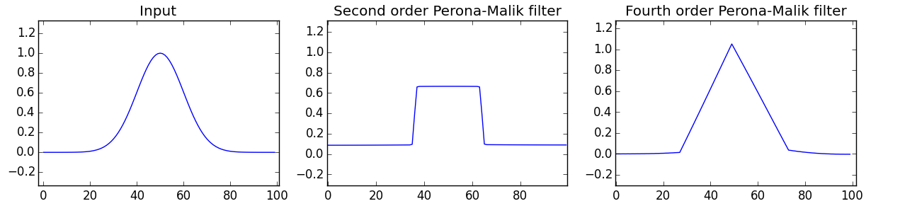
Figure 2: Second-order diffusion filter and fourth-order diffusion filter applied on a 1-D input signal. Both filters use the Perona-Malik diffusivity function.

Figure 2 shows a simple one-dimensional example with the Perona-Malik diffusivity function (1). The edge enhancement of nonlinear second-order diffusion, which leads to a piecewise constant result, and the curvature enhancement of nonlinear fourth-order diffusion, which leads to a piecewise linear result, are clearly visible. Obviously, localizing the maximum will be much easier and more reliable in case of the sharp peak created by fourth-order diffusion than in the extended plateau that results from second-order diffusion.

It is this curvature-enhancing property of fourth-order diffusion that we exploit in our novel filter. We combine it with the idea of anisotropic diffusion, which was introduced to image processing by Weickert weickert1998anisotropic to address another limitation of the Perona-Malik model. Namely, a consequence of preserving edges by locally reducing the amount of smoothing is that the neighborhoods of edges remain noisy. Anisotropic diffusion $\partial_{t}u=\mathrm{div}(D\,\nabla_{\mathbf{x}}u)$ replaces the scalar diffusivity $g$ by a second-order diffusion tensor $D$, which makes it possible to reduce smoothing orthogonal to, but not along image features, and therefore to denoise edges more effectively than isotropic nonlinear diffusion, while still avoiding to destroy them.

We generalize this approach to a novel anisotropic fourth-order diffusion equation that smoothes along the crease, while creating a sharp peak in the orthogonal direction, to clearly indicate its center. We are aware of only one previous formulation of anisotropic fourth order diffusion, proposed by Hajiaboli hajiaboli2011anisotropic . However, it has been designed to preserve edges, rather than enhance creases. Consequently, it is not well-suited for our purposes, as we will demonstrate in the results. Moreover, it differs from our approach in that it does not make use of a fourth-order diffusion tensor, and includes no mechanism for scale selection.

Despite the long history of research in this area, improved filtering and detection of ridges continues to be an active topic in medical image analysis. Our work on improving localization through fourth-order diffusion complements recent advances. For example, the SCIRD ridge detector by Annunziata et al. annunziata2015scale , or the vesselness measure by Jerman et al. jerman2016enhancement that gives better responses for vessels of varying contrasts, could replace the vessel segmentation by Frangi et al. frangi1998multiscale that we use as a prefiltering step. Several recent works franken2009crossing ; hannink2014crossing ; scharr2012short ; stuke2004analysing have addressed diffusion in crossings and bifurcations, and could be combined with our work to improve the performance of our filter in such cases.

3 Method

3.1 Anisotropic Fourth-order Diffusion

Building on work of Lysaker et al. lysaker2003noise , Didas et al. didas2009properties formulate nonlinear fourth-order diffusion as

$$\partial_{t}u= -\partial_{xx}(g(\|H(u)\|_{F}^{2})u_{xx})-\partial_{yx}(g(\|H(u)\|_{F}^{2})u_{xy})$$ (3)

$$-\partial_{xy}(g(\|H(u)\|_{F}^{2})u_{yx})-\partial_{yy}(g(\|H(u)\|_{F}^{2})u_{yy})\text{,}$$

where $\|H(u)\|_{F}^{2}$ is the Frobenius norm of the Hessian matrix of image $u$, and $u_{xy}=\partial_{xy}u$. We propose the following novel anisotropic fourth-order diffusion model, which combines the ideas of higher-order diffusion with that of making diffusivity a function of both spatial location and direction:

$$\partial_{t}u= -\partial_{xx}\left[\mathcal{D}(H_{\rho}(u_{\sigma})):H(u)\right]_{xx}$$ (4)

$$-\partial_{yx}\left[\mathcal{D}(H_{\rho}(u_{\sigma})):H(u)\right]_{xy}$$

$$-\partial_{xy}\left[\mathcal{D}(H_{\rho}(u_{\sigma})):H(u)\right]_{yx}$$

$$-\partial_{yy}\left[\mathcal{D}(H_{\rho}(u_{\sigma})):H(u)\right]_{yy}\text{.}$$

Equation (4) introduces a general linear map $\mathcal{D}$ from the Hessian matrix $H$ to a transformed matrix. Linear maps from matrices to matrices are naturally written as fourth-order tensors, and we use the “double dot product” $\mathcal{D}:H$ as a shorthand for applying the map $\mathcal{D}$ to the Hessian matrix $H$. This results in a transformed matrix $T$, and we use square brackets $[T]_{ij}$ to denote its $(i,j)$th component. Formally,

$$\left[T\right]_{ij} =\left[\mathcal{D}(H_{\rho}(u_{\sigma})):H(u)\right]_{ij}$$ (5)

$$=\sum_{k=1}^{2}\sum_{l=1}^{2}\left[\mathcal{D}(H_{\rho}(u_{\sigma}))\right]_{ijkl}\left[H(u)\right]_{kl}.$$

In this notation, we can define second-order eigentensors $E$ of $\mathcal{D}$ corresponding to eigenvalue $\mu$ by the equation $\mathcal{D}:E=\mu E$. An alternative notation, which will be used for the numerical implementation in Section 3.4, writes the Hessian and transformed matrices as vectors. This turns $\mathcal{D}$ into a matrix whose eigenvectors are nothing but the vectorized eigentensors as defined above. Similar to others Basser:2007 ; Kindlmann:2007 , we find the fourth-order tensor and “double dot” notation more appealing for reasoning at a higher level, because it allows us to preserve the natural structure of the involved matrices.

Using our square bracket notation, an equivalent way of writing one of the terms from Equation (3), $\partial_{ji}(g(\|H(u)\|_{F}^{2})u_{ij})$, is $\partial_{ji}\left[g(\|H(u)\|_{F}^{2})H(u)\right]_{ij}$. Thus, the difference between the model from Equation (3) and our new one in Equation (4) is to replace the isotropic scaling of Hessian matrices using a scalar diffusivity $g$, with a general linear transformation $\mathcal{D}$, which acts on the second-order Hessian in analogy to how the established second-order diffusion tensor acts on gradients in second-order anisotropic diffusion. Due to this analogy, we call $\mathcal{D}$ a fourth-order diffusion tensor.

In our filter, $\mathcal{D}$ is a function of the local normalized Hessians, which are defined as

$$H_{\rho}(u_{\sigma})=G_{\rho}\ast\left(\frac{1}{\sqrt{1+\left\|\nabla u_{\sigma}\right\|}}H\left(u_{\sigma}\right)\right)\text{, }$$ (6)

where regularized derivatives are obtained by convolution with a Gaussian kernel, $u_{\sigma}:=u\ast G_{\sigma}$. Its width $\sigma$ should reflect the scale of the crease, as will be discussed in Section 3.3. Since scale selection might introduce spatial discontinuities in the chosen $\sigma$, the normalized Hessians are made differentiable by integrating them over a neighborhood, for which we use a Gaussian width $\rho=0.5$ in our experiments. As shown in haralick:1983 , and used for vesselness enhancement diffusion in canero2003vesselness , the inverse gradient magnitude factor is used to make the eigenvalues of $H_{\rho}(u_{\sigma})$ match the surface curvature values.

We emphasize that, unlike in a previous generalization of structure tensors to higher order schultz2009higher , the reason for going to higher tensor order in Equation (4) is not to preserve information at crossings; this is a separate issue that was recently addressed by others hannink2014crossing , and that we plan to tackle in our own future work. In our present work, our goal is to smooth along ridges and valleys, while sharpening them in the orthogonal direction. This sharpening requires the curvature-enhancing properties of fourth-order diffusion, and a fourth-order diffusion tensor is a natural consequence of making fourth-order diffusion anisotropic.

3.2 Fourth-order Diffusion Tensor $\mathcal{D}$

We now need to construct our fourth-order diffusion tensor $\mathcal{D}$ so that it will smooth along creases, while enhancing them in the perpendicular direction. Similar to Weickert’s diffusion tensors weickert1998anisotropic , we will construct $\mathcal{D}$ in terms of its eigentensors $E_{i}$ and corresponding eigenvalues $\mu_{i}$, as defined above.

Didas et al. didas2009properties have shown that fourth-order diffusion with the Perona-Malik diffusivity perona1990scale allows for adaptive smoothing or sharpening of image curvature, depending on a contrast parameter $\lambda$. In particular, in the 1-D case, only forward diffusion (i.e., smoothing) happens in regions with $|\partial_{xx}u|<\lambda$, while only backward diffusion (i.e., curvature enhancement) occurs where $|\partial_{xx}u|>\sqrt{3}\lambda$. We wish to exploit this to enhance creases whose curvature is strong enough to begin with, while smoothing out less significant image features.

This is achieved by deriving the eigenvalues $\mu_{i}$ of $\mathcal{D}$ from the eigenvalues $\nu_{1},\nu_{2}$ of the normalized Hessian $H_{\rho}(u_{\sigma})$ using the Perona-Malik diffusivity perona1990scale , i.e.,

$$\mu_{i}=\frac{1}{1+\nu_{i}^{2}/\lambda^{2}}\text{, for }i\in\{1,2\}\text{.}$$ (7)

If the user wishes to specifically enhance either ridges or valleys, the sign of $\nu_{i}$ could be taken into account. For instance, a ridge-like behaviour in the $i$th direction is characterized by $\nu_{i}<0$. Therefore, we can decide to smooth out valleys by setting $\mu_{i}=1$ wherever $\nu_{i}\geq 0$, and enhance ridges wherever $\nu_{i}<0$ by defining $\mu_{i}$ as before. Enhancing only valleys can be done in full analogy. In our experiments on synthetic data, we found that, in terms of the $\ell_{2}$ difference between the ground truth and the filtered image, better results were obtained when enhancing both ridges and valleys. This is the setting used in all our experiments.

The ridge and valley directions can be found from the eigenvectors $e_{1},e_{2}$ of the normalized Hessian matrix $H_{\rho}(u_{\sigma})$, and are reflected in the eigentensors $E_{i}$ of $\mathcal{D}$ by setting

$$\begin{array}[]{cccc}E_{1}=&e_{1}\otimes e_{1}&E_{3}=&\frac{1}{\sqrt{2}}(e_{1}\otimes e_{2}+e_{2}\otimes e_{1})\\ E_{2}=&e_{2}\otimes e_{2}&E_{4}=&\frac{1}{\sqrt{2}}(e_{1}\otimes e_{2}-e_{2}\otimes e_{1})\end{array}\text{ .}$$ (8)

The $E_{i}$ are orthonormal with respect to the tensor dot product $A:B:=\mathrm{tr}(B^{\mathrm{T}}A)$. By definition, $E_{4}$ is antisymmetric. Since Hessians of smooth functions are symmetric, the value of $\mu_{4}$ does not play a role, and is simply set to zero. We define $\mu_{3}$ as the average of $\mu_{1}$ and $\mu_{2}$.

3.3 Scale Selection

In the previous sections, crease orientation was estimated using the eigenvectors of the regularized and normalized Hessian in Equation (6). As in previous approaches such as vesselness enhancement diffusion (VED) canero2003vesselness , this involves a regularization parameter $\sigma$ that should be adapted to the local radius of the crease. Setting this parameter is referred to as scale selection.

The vesselness measure $\mathcal{V}_{\sigma}$ by Frangi et al. frangi1998multiscale is maximal at the scale $\sigma$ that matches the corresponding vessel size, and has been widely used for detecting the local radius of vessel like structures. $\mathcal{V}_{\sigma}$ is obtained from sorted and scale-normalized eigenvalues $|\tilde{\nu}_{1}|\leq|\tilde{\nu}_{2}|$, computed as $\tilde{\nu}_{i}:=\sigma^{2}\nu_{i}$ from eigenvalues $\nu_{i}$ of the Hessian $H(u_{\sigma})$ at a given scale $\sigma$. The factor $\sigma^{2}$ compensates for the loss of contrast at larger scales lindeberg1998edge .

A vesselness measure $\mathcal{V}_{\sigma}$ should be low in background regions where overall curvature and thus $\mathcal{S}=\sqrt{\tilde{\nu}_{1}^{2}+\tilde{\nu}_{2}^{2}}$ are low overall. Moreover, it should detect tubular structures, where $|\tilde{\nu}_{1}|\ll|\tilde{\nu}_{2}|$, as opposed to blobs, in which $\mathcal{R_{B}=}\frac{\tilde{\nu}_{1}}{\tilde{\nu}_{2}}$ would be large. For ridges ($\tilde{\nu}_{2}<0$), Frangi et al. achieve this by combining $\mathcal{S}$ and $\mathcal{R_{B}}$ according to

$$\mathcal{V}_{\sigma}u=\begin{cases}0&\text{\quad if }\quad\tilde{\nu}_{2}>0\\ \left(\text{e}^{-\frac{\mathcal{R_{B}^{\mathrm{2}}}}{2\beta^{2}}}\right)\left(1-\text{e}^{-\frac{\mathcal{S}^{2}}{2c^{2}}}\right)&\text{\quad otherwise}\end{cases}\text{ ,}$$ (9)

where the $\beta$ and $c$ parameters tune $\mathcal{V}_{\sigma}u$ to be more specific with respect to suppression of blob shapes or background structures, respectively. We use $\beta=0.5$ and $c=\frac{1}{2}(\text{max}(\mathcal{S}))$, as recommended in frangi1998multiscale .

The scale for each pixel is selected as the $\sigma$ for which the maximum $\mathcal{V}u=\max_{\sigma=\sigma_{\text{min}},...,\sigma_{\text{max}}}\mbox{$\mathcal{V}_{\sigma}$$u$}$ is attained, where $\{\sigma_{\text{min}},...,\sigma_{\text{max}}\}$ are the range of expected scales in the image. For pixels that are part of the background, $\mathcal{V}u$ is low, and it can be thresholded by parameter $\theta\in\left[0,1\right]$ for vessel segmentation. This segmentation indicates the extent of vessels, and is used for our scale-image postprocessing, as described below.

It has been observed previously descoteaux2008geometric that vesselness often fails to correctly estimate the scale of the vessel along its boundary. This can happen in two cases: When the ridge has a step-like shape, the curvature near the corner points will be much larger at the finest scale than at all other scales, leading to an underestimation of the real scale near the boundary. On the other hand, the cross-sectional intensity profile of vessels may have inflection points near its edges, where $\tilde{\nu}_{2}$ changes its sign. In this case, some points near the boundary will have zero vesselness at the finest scale, but the sign of $\tilde{\nu}_{2}$ will flip, and therefore vesselness becomes non-zero, at coarser scales, leading to an overestimation of scale. Figure 3 shows both scale underestimation or overestimation at vessel boundaries.

Input	Scale Image	Post Processed

Figure 3: The color of each pixel in the scale image illustrates the scale of the underlying vessel. Artifacts near the boundaries are removed in a post processing step.

While such effects are less problematic for the VED filter, which uses the same vesselness measure for scale selection, it can lead to serious artifacts in our filter, where misestimating the scales at boundaries can cause the curvature-enhancing diffusion to enhance the boundary of large-scale ridges more than their center.

We avoid such boundary effects by introducing a novel postprocessing of the computed scales. For each pixel on a vessel, the vessel cross-section containing that pixel is extracted by following the eigenvector direction that corresponds to the strongest eigenvalue of the Hessian matrix computed at the scale suggested by the vesselness measures at each point. Then, all pixels are assigned the scale closest to the average of all pixels that lie on the same cross-section. This removes the problem of scale over- or underestimation on the boundaries. Figure 3 shows the scale image before and after being post processed.

3.4 Stability

In order to solve Equation (4), we discretize it with standard finite differences, and use an explicit numerical scheme. In matrix-vector notation, this can be written as

$$u^{k+1}=u^{k}-\tau Pu^{k}=(I-\tau P)u^{k}\text{ ,}$$ (10)

where $u^{k}\in\mathbb{R}^{m}$ is the vectorized image at iteration $k$, and the exact form of matrix $P\in\mathbb{R}^{m\times m}$ will be discussed later. We call a numerical scheme $\ell_{2}$ stable if

$$\left\|u^{k+1}\right\|_{2}\leq\left\|u^{k}\right\|_{2}\text{ ,}$$ (11)

i.e., the $\ell_{2}$ norm of the image is guaranteed not to increase from iteration $k$ to $k+1$. It follows from Equation (10) that

$$\left\|u^{k+1}\right\|_{2}\leq\left\|I-\tau P\right\|_{2}\cdot\left\|u^{k}\right\|_{2}\text{ ,}$$ (12)

where $\left\|P\right\|_{2}$ denotes the $\ell_{2}$ norm of $P$, i.e., $\left\|P\right\|_{2}:=\sqrt{\rho(P^{T}P)}$, where $\rho(P^{T}P)$ computes the largest modulus of eigenvalues of the symmetric matrix $P^{T}P$.

Consequently, the condition in Equation (12) is satisfied if

$$\left\|I-\tau P\right\|_{2}\leq 1\text{ .}$$ (13)

Since $P$ is positive semi-definite, the eigenvalues of $I-\tau P$ are within the interval $\left[1-\tau\left\|P\right\|_{2},1\right]$. Thus, Equation (13) is satisfied if $1-\tau\left\|P\right\|_{2}\geq-1$. This results in the following constraint on the permissible time step size $\tau$:

$$\tau\leq\frac{2}{\left\|P\right\|_{2}}\text{ .}$$ (14)

$k=0$, $t=0$	$k=4$, $t=20$
$k=8$, $t=40$	$k=12$, $t=60$

Figure 4: MAFOD filter applied on the noisy synthesized branch image at different FED cycles $k$. Value $t$ represents the overall diffusion time at each cycle $k$.

This clarifies that the restriction on the time step size only depends on $\left\|P\right\|_{2}$. To compute it, we will now write down the system matrix $P$ for our discretization of fourth-order anisotropic diffusion filtering.

Let $L_{xx}$, $L_{xy}$, $L_{yx}$, $L_{yy}$ be matrices approximating the corresponding derivatives. For “natural” boundary condition, it is important only to approximate the derivatives at pixels $i$ where the whole stencil fits in the image domain, i.e., where enough data is available. Let us combine these four matrices pixelwise into one big matrix $L$ such that

$$Lu\approx\left(\begin{array}[]{c}\vdots\\ \left[L_{xx}u\right]_{i}\\ \left[L_{xy}u\right]_{i}\\ \left[L_{yx}u\right]_{i}\\ \left[L_{yy}u\right]_{i}\\ \vdots\end{array}\right)\text{,}$$ (15)

i.e., the approximations of the four derivatives will be next to each other for every pixel $i$.

The $4\times 4$ matrix form of the fourth-order diffusion tensor in pixel $i$, acting on

$$\left(\left[L_{xx}u\right]_{i}\text{ }\left[L_{xy}u\right]_{i}\text{ }\left[L_{yx}u\right]_{i}\text{ }\left[L_{yy}u\right]_{i}\right)^{T},$$

can be written as $D_{i}=EME^{T}$, where $E$ is an orthogonal matrix containing the vectorized $E_{1}$, $E_{2}$, $E_{3}$, $E_{4}$ from Equation (8) as its columns and $M$ is a diagonal matrix with the eigenvalues $\mu_{1}$, $\mu_{2}$, $\mu_{3}$, $\mu_{4}$ on its diagonal. Due to the choice of the Perona-Malik diffusivity in our model, $\left\|D_{i}\right\|_{2}\leq 1$.

If we arrange all per-pixel matrices $D_{i}$ in one big matrix $D$ with a $4\times 4$ block-diagonal structure,

$$D=\left(\begin{array}[]{ccccc}D_{1}&&\cdots&&0\\ &D_{2}\\ \vdots&&D_{3}&&\vdots\\ &&&\ddots\\ 0&&\cdots&&D_{m}\end{array}\right)\text{,}$$ (16)

it is clear that $\left\|D\right\|_{2}\leq 1$, and the whole scheme reads as

$$u^{k+1}=u^{k}-\tau L^{T}DLu^{k}\text{.}$$ (17)

Substituting into Equation (14) yields

$$\tau\leq\frac{2}{\left\|L^{T}DL\right\|_{2}}\text{,}$$ (18)

meaning that, in order to find a stable step size $\tau$, we have to bound

$$\left\|L^{T}DL\right\|_{2}\leq\left\|L\right\|_{2}^{2}\leq\sum_{i,j\in\{x,y\}}\left\|L_{i,j}\right\|_{2}^{2}\text{,}$$ (19)

whose value will depend on the exact second-order finite difference stencils. We will use the same discretization as Hajiaboli hajiaboli2011anisotropic , i.e.,

$$u_{xx} \approx\frac{\left(u_{i-1,j}-2u_{i,j}+u_{i+1,j}\right)}{\left(\Delta x\right)^{2}}$$

$$u_{yy} \approx\frac{\left(u_{i,j-1}-2u_{i,j}+u_{i,j+1}\right)}{\left(\Delta y\right)^{2}}$$

$$u_{xy} \approx\frac{\left(u_{i-1,j-1}+u_{i+1,j+1}-u_{i-1,j+1}-u_{i+1,j-1}\right)}{4\Delta x\Delta y}$$

$$u_{yx} =u_{xy}\text{ ,}$$

where $\Delta x$ and $\Delta y$ are the pixel edge lengths in $x$ and $y$ directions, respectively. It is easy to verify using Gershgorin’s theorem that this results in

$$\tau\leq\frac{2}{16\left(\Delta x\right)^{2}+16\left(\Delta y\right)^{2}+2\left(\Delta x\Delta y\right)}\text{,}$$ (20)

i.e., for $\Delta x=\Delta y=1$, $\tau\leq 1/17$.

3.5 Implementation Using Fast Explicit Diffusion

Since the time step size $\tau$ derived in the previous section is rather small, solving the discretized version of Equation (4) numerically using a simple explicit Euler scheme requires significant computational effort. The recently proposed Fast Explicit Diffusion (FED) provides a considerable speedup by varying time steps in cycles, in a way that up to half the time steps within a cycle can violate the stability criterion, but the cycle as a whole still remains stable weickert2016cyclic . Consequently, a much smaller number of iterations is required to reach the desired stopping time.

The FED scheme is defined as follows:

$$\begin{array}[]{cc}u^{k+1,0}=u^{k}\text{,}\\ u^{k+1,i+1}=(I-\tau_{i}P(u_{\sigma}^{k}))u^{k+1,i}&\text{ }i=0,\ldots,n-1\text{,}\\ u^{k+1}=u^{k+1,n}\qquad\qquad\qquad\quad\text{ }\end{array}$$ (21)

where index $k$ is the cycle iterator, $i$ is the inner cycle iterator, and $n$ is the number of sub-steps in each cycle. In order to ensure stability, $P(u_{\sigma}^{k})$ must be constant during each cycle. For computing $\tau_{i}$, first the number of sub-steps in each cycle must be computed using

$$n=\left\lceil-0.5+0.5\sqrt{1+\frac{12T}{M\tau_{\text{max}}}}\right\rceil\text{,}$$ (22)

where $T$ is the diffusion stopping time, $M$ is the number of FED cycles and $\tau_{\text{max}}$ is the step size limit that ensures stability. In our experiments we set $\tau_{max}=0.05$ according to the limit computed in Section 3.4. As it is shown in weickert2016cyclic , $n$ determines $\tau_{i}$:

$$\tau_{i}=\frac{3T}{2M\left(n^{2}+n\right)\cos^{2}\left(\pi\cdot\frac{2i+1}{4n+2}\right)}\text{, }\left(i=0,\ldots,n-1\right)\text{.}$$ (23)

In order to decrease balancing error within each cycle, $\tau_{i}$’s order should be rearranged. In our experiments we have used the $\kappa$-cycles method for $\tau_{i}$ reordering weickert2016cyclic .

The fast explicit diffusion framework can be combined with our discretization in a straightforward manner, and has led to a speedup of around two orders of magnitude in some of our experiments. For both $\tau_{i}$ computation and reordering we have used the provided source code by Weickert et al. weickert2016cyclic . Figure 4 shows our filter applied on a synthesized image using the FED scheme with different cycle iterators $k$, corresponding to different stopping times.

Input	CED	VED
	$\mathcal{E}=1.096\text{, }\mathbf{p=100\%}$	$\mathcal{E}=1.116\text{, }\mathbf{p=100\%}$
IFOD	Single-scale Gaussian	Multi-scale Gaussian
$\mathcal{E}=1.579\text{, }p=96\%$	$\mathcal{E}=1.263\text{, }p=98\%$	$\mathcal{E}=0.566\text{, }\mathbf{p=100\%}$
Bilateral	Hajiaboli	MAFOD
$\mathcal{E}=0.624\text{, }p=99\%$	$\mathcal{E}=1.024\text{, }p=92\%$	$\mathbf{\mathcal{E}=0.332\text{, }p=100\%}$

Figure 5: Red curves show the ground truth ridge location, while blue curves show the location reconstructed from the filtered noisy image. Our MAFOD filter restores ridge locations from the noisy image with ridges of different scales better than other filters.

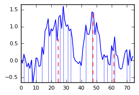
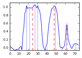
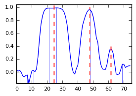
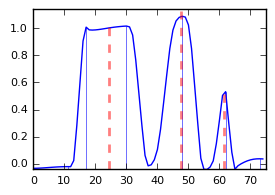
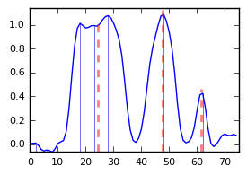
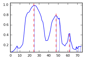
[capbesideposition=left,top,capbesidewidth=4cm]figure[] Input CED VED IFOD Single-scale Gaussian Multi-scale Gaussian Bilateral Hajiaboli MAFOD

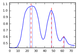
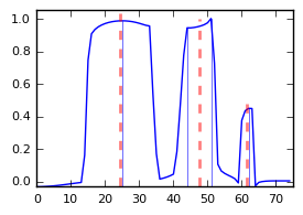
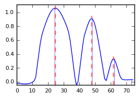
Figure 6: Each plot shows the intensities on a left to center line of the 2D images in Figure 5. The lines are taken from the middle of each image. The red dashed lines show the true position of the ridge points, and the blue lines show the position of local maxima over the intensity line scan of each filtered image.

3.6 Ridge and Valley Extraction

After enhancing ridges and valleys with our filter, we extract a polygonal representation of them using a 2D counterpart of an established 3D algorithm schultz2010crease . Our algorithm is based on the idea of marching squares schroeder2005overview and involves the zero contour of the scalar field $d=\text{det}(g|Hg)$, where $(g|Hg)$ indicates a matrix whose first column is the local gradient vector $g$ and the second column $Hg$ is the result of multiplying the gradient vector to the Hessian matrix; $\text{det}(\centerdot)$ is the matrix determinant. The zero level set of $d$ is a superset of the creases peikert2008height .

Our overall approach of ridge extraction involves two different notions of scale: The first one refers to the selection of scales at which derivatives are taken, as discussed in Section 3.3; the second one to the stopping time $t$ of our filter. To clarify their respective roles, we compare our approach to the seminal work by Lindeberg lindeberg1998edge on ridge extraction in Gaussian scale space.

In Lindeberg’s approach, ridge curves in 2D images sweep out surfaces in three-dimensional scale space, and curves on these surfaces are found along which a measure of ridge strength is locally maximal with respect to diffusion time $t$. An example of such a measure is

$$R(u_{\sigma})=t^{4\gamma}\left(u_{xx}+u_{yy}\right)^{2}\left(\left(u_{xx}-u_{yy}\right)^{2}+4u_{xy}^{2}\right)\text{.}$$ (24)

In this approach, stopping time $t$ and the scale $\sigma$ of derivatives are related by $t=\sigma^{2}/2$, and can thus be considered as one single parameter, whose value is determined automatically. The exponent $\gamma$ in the normalization factor that is used to compensate for the loss of contrast at later diffusion times is treated as a tunable parameter. In our experiments, we set it to $\gamma=\frac{3}{4}$, as proposed in lindeberg1998edge .

Decoupling the $t$ and $\sigma$ parameters is a price that we pay in our method in order to preserve and enhance creases, for which Gaussian scale space does not have any mechanism. Our current implementation selects the derivative scale $\sigma$ automatically, as discussed in Section 3.3, but does not have an objective criterion for setting the stopping time $t$, unless ground truth is available. In practice, we found it relatively simple to tune this parameter based on viewing the corresponding images, especially given that, after image noise has been removed, results are relatively stable (cf. Figure 4). Future work might investigate automated selection of this parameter.

Another difference between our approach and Lindeberg’s is that his crease extraction algorithm operates on the full scale space, while ours, similar to previous work by Barakat et al. Barakat:2011 , works on a single, pre-filtered image. Both approaches have relative benefits and drawbacks: Scale space crease extraction is challenging to implement, and requires much more time and memory, especially when dealing with the four-dimensional scale space resulting from three-dimensional input images Kindlmann:2009Vis . On the other hand, it might, in rare cases, indicate spatially intersecting creases at different scales, which our current approach is not able to reproduce.

4 Experimental Results

We compare our multi-scale anisotropic fourth-order diffusion (MAFOD) to crease enhancement diffusion (CED) sole2001crease , vesselness enhancement diffusion (VED) canero2003vesselness , isotropic fourth-order diffusion (IFOD) lysaker2003noise , the anisotropic fourth-order diffusion by Hajiaboli hajiaboli2011anisotropic , bilateral, and a multi-scale Gaussian filter. Since it was already shown in sole2001crease that the coherence enhancing diffusion filter weickert1998anisotropic tends to more strongly deform non linear structures compared to the CED filter, it is not included in the comparison.

The multi-scale Gaussian filter is defined to approximate Lindeberg’s scale selection, as described in Section 3.6. From a range of stopping times between $t=1$ and $t=30$, it first selects an optimal scale for each pixel, by finding the $t$ that maximizes $R(u_{\sigma})$ from Equation (24). Then, the intensity of each pixel in the output image is obtained by convolving the input image with a Gaussian at the locally optimal scale $\sigma=\sqrt{2t}$ that is then normalized between $\left[0,1\right]$. The normalization is necessary to compensate for the intensity range shrinkage after Gaussian blurring.

The crease extraction algorithm from Section 3.6 results in a set of polygonal chains. For each crease line segment in the ground truth, a corresponding segment in the reconstruction is selected by picking the one with minimum Hausdorff distance huttenlocher1993comparing in a neighborhood around the ground truth line segment. This neighborhood is set to six pixels for the experiments on synthetic data, and to ten pixels for real data. The average Euclidean distance $\mathcal{E}$ between the ground truth and the corresponding reconstruction is then used to quantify the accuracy of vessel locations in the filtered image. In addition to $\mathcal{E}$, we show the percentage $p$ of ground truth for which a corresponding ridge was detected from the filtered images while computing $\mathcal{E}$.

In the experiments on synthesized images, image evolution of all filters, except for multi-scale Gaussian and bilateral filters, was stopped when the $\ell_{2}$ difference between the filtered image and the noise-free ground truth was minimized. $\ell_{2}$ difference was chosen over $\mathcal{E}$ as a stopping criterion due to its much lower computational cost.

4.1 Confirming Theoretical Properties

Our filter has been designed to improve localization accuracy while accounting for creases at multiple scales and being rotationally invariant. Results on a simple simulated image with three concentric ridges of different radii, which is contaminated with zero-mean Gaussian noise with a signal to noise ratio $\mathrm{SNR}=6.81$, verify that these design goals are met.

Both Figure 5 and Figure 6 show that our MAFOD filter restores ridge locations most accurately as assessed both by visual inspection and Euclidean distance $\mathcal{E}$. MAFOD outperforms CED, IFOD, Hajiaboli and bilateral filtering since it accounts for different scales. On the other hand, the curvature enhancement of our filter, which is not part of multiscale VED or Gaussian filters, clearly makes it easier for the ridge extraction algorithm to localize the centerline, especially in the largest ridge. IFOD does perform curvature enhancement but, due to its isotropic nature, it is not effectively guided to act specifically across the ridge. As it is obvious on the largest circle, the multi-scale Gaussian filter leads to ridge displacement. The result of the anisotropic fourth-order filter by Hajiaboli clearly illustrates the fact that it was designed to preserve edges, not to enhance creases.

Ground Truth	CED	VED
	$\mathcal{E}=0.343\text{, }p=98\%$	$\mathcal{E}=0.345\text{, }\mathbf{p=100\%}$
Multi-scale Gaussian	Bilateral	MAFOD
$\mathcal{E}=0.506\text{, }p=97\%$	$\mathcal{E}=0.341\text{, }\mathbf{p=100\%}$	$\mathbf{\mathcal{E}=0.302\text{, }p=100\%}$

Figure 7: In a simulated occluded vessel, restored (blue) curves again best match the (red) ground truth locations in case of our MAFOD filter. In addition, MAFOD better preserves the occlusions than VED.

For the MAFOD filter, scales $\sigma$ and vesselness threshold $\theta$ are the same as for VED, $\sigma=\{0.5,1.0,...,8.5,9.0\}$, $\theta=0.2$. Other parameters are $\lambda=0.005$ for MAFOD, IFOD, and $\sigma=1.0$ for IFOD; for Hajiaboli, $\lambda=0.01$; for CED, $\sigma=2.0$ and it is set to enhance both ridges and valleys; for single-scale Gaussian smoothing, $\sigma=1.25$. For the MAFOD filter, FED stopping time is set to $500$, and the number of cycles is set to $10000$. For other fourth-order equations $\tau=0.03$ and for the second-order diffusion equations such as the VED and CED filters, $\tau=0.2$; for the bilateral filter $\sigma_{spatial}=3.0$ and $\sigma_{range}=1.0$.

4.2 Simulated Vessel Occlusion

Figure 7 shows a second image, simulating an occluded vessel, and corrupted with Gaussian noise with $\mathrm{SNR}=6.40$. Our MAFOD filter leads to the most accurate localization in terms of Euclidean error $\mathcal{E}$. In particular, we observed that VED widens the occlusions. They are better preserved by our filter, which we set to enhance both ridges and valleys.

Again, an amount of smoothing that minimized $\ell_{2}$ error was used for all filters except for multi-scale Gaussian and bilateral filters. The parameters for VED and MAFOD are $\sigma=\{0.5,1.0,1.5,2.0,2.5,3.0\}$, and $\theta=0.35$; $\lambda=0.017$, stopping time is $20$ and the number of cycles is set to $1000$ for MAFOD; for CED, $\sigma=1.0$; for the bilateral filter, $\sigma_{\text{spatial}}=1.5$ and $\sigma_{\text{range}}=1.0$. For the numerical solver, we set $\tau=0.05$ for the fourth-order equation and for second-order equations, $\tau=0.2$.

4.3 Real Vessel Tree

To demonstrate our filter on a real-world example, we applied it to several ROIs from an infrared fundus image, on which one of our co-authors (MWMW), who is an ophthalmologist, manually marked the exact vessel locations to provide a ground truth for comparison, without being shown the filtered images. Results in Figure 8 show that our MAFOD filter outperforms VED, multi-scale Gaussian and bilateral filters in restoring vessel locations. In ROI 3, at some point the two thickest vessels run close to each other. By looking at the filtered image with the VED, the two vessels are erroneously connected to each other in that area, even though they are not connected in the corresponding extracted valley curves. Our MAFOD filter correctly avoided connecting the vessels to each other.

Even though vessels generally appear dark (i.e., as valleys) in these images, the larger ones exhibit a thin ridge at their center, due to a reflex in the infrared image. This leads to an incorrect double response in single-scale filters as shown for the bilateral filter. CED and IFOD filters suffer from similar problems (results not shown).

For each filter separately, we carefully tuned the parameters for optimum results. Specially $\theta$, $\lambda$ and the stopping time are the parameters that need more careful tuning compared to others. For the MAFOD filter, we set $\sigma=\{0.2,0.3,0.5,1.0,...,6.5,7.0\}$, $\lambda=0.005$, $\theta=0.13$, and used a FED scheme with stopping time $12$ and cycle number $2$. For the VED filter, an explicit Euler scheme is used with $600$ iterations and $\tau=0.2$, and the same parameters for scale selection as for MAFOD; for the bilateral filter, $\sigma_{\text{range}}=0.3$ and $\sigma_{\text{spatial}}=3.0$; for the multi-scale Gaussian filter an additional Gaussian smoothing with kernel size $\sigma=2$ is applied to the filtered image to blur out discontinuities from scale selection and thus achieve an even better result. The computational effort of all filters is reported in Table 1.

Input	VED filter	Bilateral Filter	Ms Gaussian	MAFOD filter
ROI 1	$\mathcal{E}=1.45$	$\mathcal{E}=1.36$	$\mathcal{E}=1.89$	$\mathbf{\mathcal{E}=1.17}$
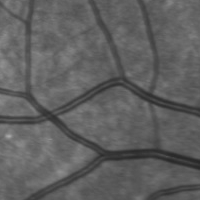
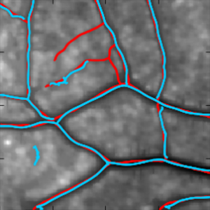
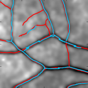
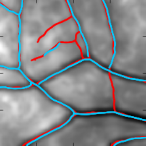
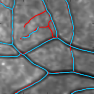
ROI 2	$\mathcal{E}=1.31$	$\mathcal{E}=1.42$	$\mathcal{E}=1.27$	$\mathbf{\mathcal{E}=1.04}$
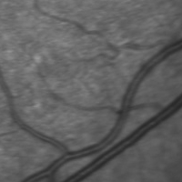
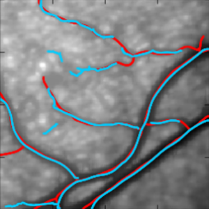
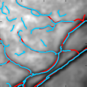
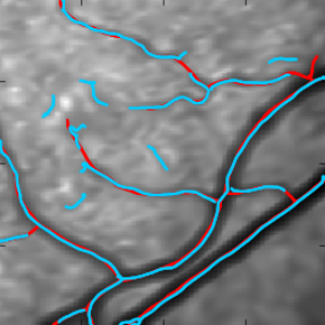
ROI 3	$\mathcal{E}=1.43$	$\mathcal{E}=1.63$	$\mathcal{E}=1.62$	$\mathbf{\mathcal{E}=1.15}$
	$p=89\%$	$p=80\%$	$p=88\%$	$\mathbf{p=92\%}$

Figure 8: In three ROIs of a fundus image, reconstructed vessel locations (blue) best match a manually marked ground truth (red) when our MAFOD filter is used.

Table 1: The average filtering time for a single ROI of size $200\times 200$ pixels in Figure  8.

Filter	VED	Bilateral	Ms Gaussian	MAFOD
Time ($sec$)	$1251$	$0.16$	$2.24$	$6.51$

5 Conclusion

We have proposed a new multi-scale fourth order anisotropic diffusion (MAFOD) filter to enhance ridges and valleys in images. It uses a fourth order diffusion tensor which smoothes along creases, but sharpens them in the perpendicular direction, and optionally enables enhancing either ridges or valleys only. Our results indicate that the curvature enhancing properties of fourth-order diffusion allow our filter to better restore the exact crease locations than traditional methods. In addition, we found that our filter better preserves vessel occlusions.

In the future, we would like to extend our 2-D filter to 3-D images, and to better handle crossings and bifurcations hannink2014crossing .

References

- [1] R. Annunziata, A. Kheirkhah, P. Hamrah, and E. Trucco. Scale and curvature invariant ridge detector for tortuous and fragmented structures. In Proc. Medical Image Computing and Computer-Assisted Intervention (MICCAI), Part III, volume 9351 of LNCS, pages 588–595. Springer, 2015.
- [2] S. Barakat, N. Andrysco, and X. Tricoche. Fast extraction of high-quality crease surfaces for visual analysis. Computer Graphics Forum, 30(3):961–970, 2011.
- [3] P. J. Basser and S. Pajevic. Spectral decomposition of a 4th-order covariance tensor: Applications to diffusion tensor MRI. Signal Processing, 87:220–236, 2007.
- [4] C. Caero and P. Radeva. Vesselness enhancement diffusion. Pattern Recognition Letters, 24(16):3141–3151, 2003.
- [5] M. Descoteaux, D. L. Collins, and K. Siddiqi. A geometric flow for segmenting vasculature in proton-density weighted mri. Medical image analysis, 12(4):497–513, 2008.
- [6] S. Didas, J. Weickert, and B. Burgeth. Properties of higher order nonlinear diffusion filtering. Journal of Mathematical Imaging and Vision, 35(3):208–226, 2009.
- [7] D. H. Eberly and S. M. Pizer. Ridge flow models for image segmentation. In Medical Imaging 1994, volume 2167, pages 54–64. International Society for Optics and Photonics, 1994.
- [8] A. F. Frangi, W. J. Niessen, K. L. Vincken, and M. A. Viergever. Multiscale vessel enhancement filtering. In Proc. Medical Image Computing and Computer-Assisted Interventation (MICCAI), volume 1496 of LNCS, pages 130–137. Springer, 1998.
- [9] E. Franken and R. Duits. Crossing-preserving coherence-enhancing diffusion on invertible orientation scores. International Journal of Computer Vision, 85(3):253, 2009.
- [10] J. B. Greer, A. L. Bertozzi, and G. Sapiro. Fourth order partial differential equations on general geometries. Journal of Computational Physics, 216(1):216–246, 2006.
- [11] M. R. Hajiaboli. An anisotropic fourth-order diffusion filter for image noise removal. International Journal of Computer Vision, 92(2):177–191, 2011.
- [12] J. Hannink, R. Duits, and E. Bekkers. Crossing-preserving multi-scale vesselness. In Proc. Medical Image Computing and Computer-Assisted Intervention (MICCAI), Part II, volume 8674 of LNCS, pages 603–610. Springer, 2014.
- [13] R. M. Haralick, L. T. Watson, and T. J. Laffey. The topographic primal sketch. Int’l Journal of Robotics Research, 2(1):50–72, 1983.
- [14] D. P. Huttenlocher, G. Klanderman, and W. J. Rucklidge. Comparing images using the Hausdorff distance. IEEE Trans. on Pattern Analysis and Machine Intelligence, 15(9):850–863, 1993.
- [15] T. Jerman, F. Pernuš, B. Likar, and Ž. Špiclin. Enhancement of vascular structures in 3D and 2D angiographic images. IEEE Trans. on Medical Imaging, 35(9):2107–2118, 2016.
- [16] G. Kindlmann, D. Ennis, R. Whitaker, and C.-F. Westin. Diffusion tensor analysis with invariant gradients and rotation tangents. IEEE Trans. on Medical Imaging, 26(11):1483–1499, 2007.
- [17] G. Kindlmann, R. San José Estépar, S. M. Smith, and C.-F. Westin. Sampling and visualizing creases with scale-space particles. IEEE Trans. on Visualization and Computer Graphics, 15(6):1415–1424, 2009.
- [18] T. Lindeberg. Edge detection and ridge detection with automatic scale selection. International Journal of Computer Vision, 30(2):117–156, 1998.
- [19] M. Lysaker, A. Lundervold, and X.-C. Tai. Noise removal using fourth-order partial differential equation with applications to medical magnetic resonance images in space and time. IEEE Trans. on Image Processing, 12(12):1579–1590, 2003.
- [20] R. Peikert and F. Sadlo. Height ridge computation and filtering for visualization. In IEEE Pacific Visualization Symposium, pages 119–126, March 2008.
- [21] P. Perona and J. Malik. Scale-space and edge detection using anisotropic diffusion. IEEE Trans. on Pattern Analysis and Machine Intelligence, 12(7):629–639, 1990.
- [22] P. Peter, L. Kaufhold, and J. Weickert. Turning diffusion-based image colorization into efficient color compression. IEEE Trans. on Image Processing, 26(2):860–869, 2017.
- [23] H. Scharr and K. Krajsek. A short introduction to diffusion-like methods. In Mathematical Methods for Signal and Image Analysis and Representation, pages 1–30. Springer, 2012.
- [24] O. Scherzer. Denoising with higher order derivatives of bounded variation and an application to parameter estimation. Computing, 60(1):1–27, Mar. 1998.
- [25] W. J. Schroeder and K. M. Martin. Overview of visualization. The Visualization Handbook, pages 3–35, 2005.
- [26] T. Schultz, H. Theisel, and H.-P. Seidel. Crease surfaces: From theory to extraction and application to diffusion tensor MRI. IEEE Trans. on Visualization and Computer Graphics, 16(1):109–119, 2010.
- [27] T. Schultz, J. Weickert, and H.-P. Seidel. A higher-order structure tensor. In D. H. Laidlaw and J. Weickert, editors, Visualization and Processing of Tensor Fields – Advances and Perspectives, pages 263–280. Springer, 2009.
- [28] A. F. Sóle, A. López, and G. Sapiro. Crease enhancement diffusion. Computer Vision and Image Understanding, 84(2):241–248, 2001.
- [29] I. Stuke, T. Aach, E. Barth, and C. Mota. Analysing superimposed oriented patterns. In IEEE Southwest Symposium on Image Analysis and Interpretation, pages 133–137, 2004.
- [30] J. Tumblin and G. Turk. LCIS: A boundary hierarchy for detail-preserving contrast reduction. In Proc. Annual Conference on Computer Graphics and Interactive Techniques (SIGGRAPH), pages 83–90, 1999.
- [31] G. W. Wei. Generalized perona-malik equation for image restoration. IEEE Signal Processing Letters, 6(7):165–167, 1999.
- [32] J. Weickert. Anisotropic diffusion in image processing. Teubner Stuttgart, 1998.
- [33] J. Weickert, S. Grewenig, C. Schroers, and A. Bruhn. Cyclic schemes for PDE-based image analysis. International Journal of Computer Vision, 118(3):275–299, 2016.
- [34] E. T. Whittaker. On a new method of graduation. Proceedings of the Edinburgh Mathematical Society, 10:63–75, 1922.
- [35] Y.-L. You and M. Kaveh. Fourth-order partial differential equations for noise removal. IEEE Trans. on Image Processing, 9(10):1723–1730, Oct. 2000.