DESY-16-223 Gluon momentum fraction of the nucleon from lattice QCD

Abstract

We perform a direct calculation of the gluon momentum fraction of the nucleon, taking into account the mixing with the corresponding quark contribution. We use maximally twisted mass fermion ensembles with $N_{f}=2+1+1$ flavors at a pion mass of about $370\,\mathrm{MeV}$ and a lattice spacing of $a\approx 0.082\,\mathrm{fm}$ and with $N_{f}=2$ flavors at the physical pion mass and a lattice spacing of $a\approx 0.093\,\mathrm{fm}$. We employ stout smearing to obtain a statistically significant result for the bare matrix elements. In addition, we perform a lattice perturbative calculation including 2 levels of stout smearing to carry out the mixing and the renormalization of the quark and gluon operators. We find, after conversion to the $\overline{\mathrm{MS}}$ scheme at a scale of $2\,\mathrm{GeV}$, $\langle x\rangle^{R}_{g}{=}0.284(27)(17)(24)$ for pion mass of about $370\,\mathrm{MeV}$ and $\langle x\rangle^{R}_{g}{=}0.267(22)(19)(24)$ for the physical pion mass. In the reported numbers, the first parenthesis indicates statistical uncertainties. The numbers in the second and third parentheses correspond to systematic uncertainties due to excited states contamination and renormalization, respectively.

1 Introduction

The lattice calculation of moments of quark distribution functions has matured much in the last years, as can be seen in the reviews of [1, 2], for instance. In order to include disconnected singlet contributions, present works employ large statistics [3, 4] and even computations for nucleon observables directly at the physical value of the pion mass [5].

For these moments, a complete non-perturbative renormalization program has been developed and applied in practice. Furthermore, first attempts to compute the quark distributions directly on the lattice have recently been initiated [6, 7, 8]. All these activities by lattice groups working on nucleon structure open the exciting prospect that lattice calculations will eventually provide precise results for various nucleon moments, charges and form factors with high statistics and systematic effects under control.

While the computations concerning the quark distribution functions are approaching a satisfactory situation, the case of the gluon contributions is much less advanced. In fact, presently only a few quenched results for the gluon momentum fraction (GMF) exist [10, 11, 12, 13]. This is a rather unfortunate situation since the analysis of phenomenological parton distribution functions data [14] suggests that at a scale of 6.25 $\text{GeV}^{2}$ for instance, all the quarks only contribute a fraction of about 60 percent to the total nucleon momentum. This implies that gluons carry an essential part of the nucleon momentum, in order to satisfy the sum rule

$$\sum_{q}\langle x\rangle_{q}+\langle x\rangle_{g}=1\,.$$ (1)

Moreover, the phenomenological estimates of $\langle x\rangle_{g}$ have a significantly larger uncertainty than the corresponding quark moments. The GMF will also be an important input for the computation of the gluon contribution to the nucleon spin.

In this work we perform a calculation of the lowest moment $\langle x\rangle_{g}$ of the gluon distribution function $f_{g}(x)$ using lattice QCD within the maximally twisted mass formulation [15, 16]. We will use gluon field configurations at a pion mass of about $370\,\mathrm{MeV}$ but also at the physical pion mass.

The key to obtain results for the GMF is a combination of high statistics, the use of smeared operators (cf. [17]) and the application of a suitable renormalization scheme that takes the mixing of the gluon operator with the corresponding quark singlet operator into account. The last step is presently done perturbatively but could be extended non-perturbatively in the future. We will see that employing these steps will allow us to provide a quantitative result for $\langle x\rangle_{g}$ with dynamical quarks for the first time. A first account of our results has been discussed in Ref. [18].

2 Theoretical setup

The gluon momentum fraction of a nucleon state $\langle P|$ with 4-momentum $P^{\mu}$ can be extracted from matrix elements of the gluonic QCD energy momentum tensor, see e.g. [19]

$$\langle P|T^{\{\mu\nu\}}_{g}|P\rangle=2\langle x\rangle_{g}P^{\{\mu}P^{\nu\}}\,,$$ (2)

where the normalization $\langle P|P\rangle=2E_{N}$ is used and $\{\dotsm\}$ represents symmetrization and subtraction of the trace. $E_{N}$ is the energy of the nucleon. The gluonic energy momentum tensor itself is defined as

$$T^{\{\mu\nu\}}_{g}=\frac{1}{4}g^{\mu\nu}G_{\alpha\beta}G^{\alpha\beta}-G^{\mu\sigma}{G^{\nu}_{\sigma}},$$ (3)

where $G_{\mu\nu}=T^{a}G^{a}_{\mu\nu}$ is the field strength tensor.

Based on the conventions used in [10], we construct the gluon operator

$$\mathcal{O}_{\mu\nu}=2\,{\rm Tr}[G_{\mu\sigma}G_{\nu\sigma}]$$ (4)

which contains the vector ${\mathcal{O}_{A}}_{i}$ and scalar ${\mathcal{O}_{B}}$ operators

$${\mathcal{O}_{A}}_{i}=\mathcal{O}_{i4}\hskip 14.22636pt\mathrm{and}\hskip 14.22636pt\mathcal{O}_{B}=\mathcal{O}_{44}-\frac{1}{3}\mathcal{O}_{jj}\,.$$ (5)

Here and in the following equations there is an implicit trace over the color indices of the field strength tensor and later also the plaquette term. With Eq. (2) the matrix elements of these operators can be directly related to the GMF as

$$\langle P|\mathcal{O}_{Ai}|P\rangle =i4E_{N}P_{i}\langle x\rangle_{g}$$ (6)

$$\langle P|\mathcal{O}_{B}|P\rangle =(-4\,E^{2}_{N}-\frac{2}{3}{{\mathbf{P}}}^{2})\langle x\rangle_{g}\,.$$ (7)

Eq. (6) indicates that in order to extract the GMF from matrix elements of $\mathcal{O}_{A}$, a non-zero momentum for the nucleon fields is required, whereas the kinematic factor for the operator $\mathcal{O}_{B}$ stays finite for zero momentum. Thus, for zero momentum the form factor can be extracted as

$$\frac{\langle P|\mathcal{O}_{B}|P\rangle}{\langle P|P\rangle}=-2\,m_{N}\,\langle x\rangle_{g}\,.$$ (8)

Earlier calculations, see e.g. [20, 21], showed that employing a non-zero momentum in the definition of the operator corresponding to the first moment of the quark distribution leads to a significantly enhanced noise-to-signal ratio. We therefore have chosen the operator $\mathcal{O}_{B}$ for the current calculation. We nevertheless plan a test of the operator $\mathcal{O}_{A}$ in the future.

Utilizing Eq. (4), the operator $\mathcal{O}_{B}$ can be expressed in terms of the field strength tensor as

$$\mathcal{O}_{B}=-\frac{4}{3}\left(\sum_{j<k}\,G_{jk}^{2}-\sum_{i}\,G_{4i}^{2}\right)\,.$$ (9)

This expression can now be transferred to the lattice definition of the GMF using the operator $\mathcal{O}_{B}$ through plaquette terms,

$$\mathcal{O}_{B}=-\frac{4}{9}\frac{\beta}{a^{4}}\left(\sum_{i}\mathrm{Re}(U_{i4})-\sum_{i<j}\mathrm{Re}(U_{ij})\right)\,.$$ (10)

The operator in Eq. (10) involves two terms which are very similar in magnitude and have to be subtracted. This points to the expectation that in order to obtain a precise result a high statistics and an estimate of the correlation between these two terms are required.

3 Lattice calculation

In [18] we discussed the approach of employing the Feynman-Hellmann theorem to compute the gluon momentum fraction. We demonstrated that using the Feynman-Hellmann theorem is in principle feasible but it would require a substantial effort to obtain accurate results. Thus, we instead follow the path of using the direct computation of the left-hand side of Eq. (8). This amounts to computing the ratio of a three- and a two-point correlation function

$$R(t,\tau,t^{\prime})=-\frac{1}{2\,m_{N}}\frac{C^{\text{3pt}}(t,\tau,t^{\prime};{\bf P}=0)}{C^{\text{2pt}}(t,t^{\prime};{\bf P}=0)}\stackrel{{\scriptstyle t<\tau<t^{\prime}}}{{=}}\langle x\rangle_{g}\,.$$ (11)

The space-time points $({\bf x},t),({\bf x^{\prime}},t^{\prime}),({\bf y,}\tau)$ denote the sink, source and operator insertion, respectively.

For the GMF, the relevant three-point function is the expectation value of two nucleon fields and the operator $\mathcal{O}_{B}$ from Eq. (5), and the two-point function is defined in the usual way,

$$C^{\text{3pt}}(t,\tau,t^{\prime};{\bf P}=0) =\sum_{\bf x,y}\Gamma^{+}\left\langle N(x)\mathcal{O}_{B}(y)\overline{N}(x^{\prime})\right\rangle\,,$$ (12)

$$C^{\text{2pt}}(t,t^{\prime};{\bf P}=0) =\sum_{\bf x}\Gamma^{+}\left\langle N(x)\overline{N}(x^{\prime})\right\rangle\,,$$ (13)

where $\Gamma^{+}=\frac{1+\gamma_{4}}{2}$ is the parity plus projector and the standard definition for the nucleon interpolating fields is used (cf. [5]). A schematic picture of the structure of the three-point function is shown in Fig. 1.

Figure 1: Schematic picture of Wick contractions for the three-point functions with a disconnected gluon loop.

Because there are no quark fields in the operator, the three-point function can be written as the expectation value of a product of a nucleon two-point function with a gauge link dependent operator. Generally, we call this a disconnected correlation function. Consequently, already existing two-point functions can be re-used while only the gluon operator has to be calculated on the very same configurations with a relatively small computational effort. In order to have an improved signal-to-noise ratio, we subtract the vacuum expectation value of $\mathcal{O}_{B}$ from the ratio, although strictly speaking this is not necessary since the expectation value of $\mathcal{O}_{B}$ vanishes.

To extract the matrix element of interest three methods have been employed. The simplest one is the plateau method where one must identify a time independent window in the ratio of Eq. (11). This method assumes just one-state dominance. The second method is the two-state method, where the first excited state is taken into account. Inserting a complete set of states and keeping terms up to the first excited state, the ratio becomes

$$R(t,\tau,t^{\prime})=\frac{A_{00}+A_{01}\left(e^{-\delta E_{1}(t-\tau)}+e^{-\delta E_{1}(\tau-t^{\prime})}\right)+A_{11}e^{-\delta E_{1}(t-t^{\prime})}}{1+c_{1}e^{-\delta E_{1}(t-t^{\prime})}},$$ (14)

where $A_{00}$ is the matrix element of interest and $\delta E_{1}$ is the energy gap between the ground state and the first excited state. The third method, which allows us to control better the excited states, is called the summation method. Summing over the insertion time $\tau$ of the ratio in Eq. (11), we obtain

$$R^{\rm sum}(t-t^{\prime})=\sum_{\tau=t^{\prime}+1}^{(t-1)}R(t,\tau,t^{\prime})=C+(t-t^{\prime})A_{00}+\mathcal{O}(e^{-\delta E1(t-t^{\prime})})$$ (15)

where the unphysical contact terms are discarded from the sum. From the slope of the linear fit one can extract the matrix element.

4 Lattice setup

Our first benchmark calculation is based on 2298 gluon field configurations on a $32^{3}\times 64$ lattice from an ETMC (European Twisted Mass Collaboration) production ensemble [22], labeled B55.32. It features $N_{f}=2+1+1$ flavors of maximally twisted mass fermions, i.e. two mass degenerate light quarks and non-degenerate strange and charm quarks. The ensemble has a bare coupling corresponding to $\beta=1.95$, which yields a lattice spacing of $a\approx 0.082$ fm [23] and the twisted mass parameter $a\mu=0.0055$, which corresponds to a pion mass of $m_{PS}\approx 370$ MeV. For the two-point function, 15 different source positions are used on each of the 2298 gauge field configurations. This sums up to 34470 measurements, each for proton, neutron and two different time directions.

We also include a second ensemble obtained at the physical value of the pion mass [24], which is labeled cA2.09.48. Here $N_{f}=2$ flavors of maximally twisted mass fermions are employed, together with a clover term with coefficient $c_{sw}=1.57551$ on a $48^{3}\times 96$ lattice. The bare coupling corresponds to $\beta=2.1$, which leads to a lattice spacing of $a\approx 0.093$ fm, set with the nucleon mass [5]. The twisted mass parameter is set to $a\mu=0.0009$, which corresponds, within errors, to a setup with physical pion masses. The analysis is done on 2094 configurations with 100 different source positions each, which amounts to a total of 209400 measurements.

	$N_{f}$	$\beta$	$\nicefrac{{L}}{{a}},\nicefrac{{T}}{{a}}$	$c_{sw}$	$\kappa$	$a\mu$	$m_{\text{PS}}$	$a$	measurements
							[MeV]	[fm]
B55.32	2+1+1	1.95	32,64	0	0.161236	0.0055	370	0.082	34470
cA2.09.48	2	2.1	48,96	1.57551	0.13729	0.0009	130	0.093	209400

Table 1: Parameters of two different gauge ensembles that are used in the computation of the GMF. We also give the number of measurements used for the computation.

For the quark fields that make up the nucleon interpolating field, standard smearing methods (Gaussian and Array Processor Experiment (APE) ) were used, which are known to increase the overlap of the interpolating fields with the nucleon ground state while decreasing the overlap with excited states and thus improving the results for nucleon spectroscopy and structure, cf. [25] and references therein.

5 Bare results and stout smearing

In our first attempt to compute the GMF directly we applied the gluon operator $\mathcal{O}_{B}$ from Eq. (10) without any additional smearing. However, in this setup we were not able to detect any signal despite the large statistics of 34470 measurements on the B55.32 ensemble, cf. Table 1, see Fig. 2 in [18].

One possible solution to overcome the low signal-to-noise problem has been suggested in [17], where the authors propose to use Hypercubic (HYP) smearing [26] for the gauge links in the gluon operator. However, HYP smearing is a non-analytic procedure; this fact raises some conceptual issues, and it also implies that the perturbative lattice calculation for the desired renormalization functions would be very cumbersome. In the framework of this work we have tested both HYP (up to 5 steps) and stout smearing (up to 10 steps). Results with increased stout smearing are compatible with result produced with a smaller number of HYP smearing steps. Increasing the number of smearing steps may result in contact-term contamination, which should be also assessed. Furthermore, the influence of contact terms will be reduced by increasing the source-sink separation. To test for this effect we take $t_{s}$ up to 15$a$ and we find that the results are compatible with smaller value, e.g. $t_{s}{=}10a$. Thus, we expect that contact-term contamination is small.

Thus, we switch to stout smearing of the gauge links, as introduced in [27]. This is an analytic link smearing technique where the gauge links are smeared according to

$$U_{\mu}^{(n+1)}=\exp\left(iQ_{\mu}^{(n)}\right)U_{\mu}^{(n)}\,,$$ (16)

where $Q_{\mu}$ is a particular linear combination of perpendicular gauge link staples that are weighted with the factor $\omega$, cf. [27] for details. Here, we use the isotropic four-dimensional scheme and $\omega$ is tuned so that the plaquette reaches a maximal value for a given number of smearing steps.

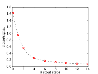
Figure 2: Inverse signal-to-noise ratio as a function of the number of stout smearing steps. The ratio shown here is the average error of plateau values divided by the result of a plateau fit for 10 steps of smearing. All results are given for a source-sink separation of $t_{s}/a=10$. Here the B55.32 ensemble was used, cf. Table 1.

We tested the effect of stout smearing on the signal-to-noise ratio by applying up to 14 smearing steps. To this end, we computed the average error of the plateau values for each level of smearing normalized by the plateau value that was extracted using 10 steps of smearing. The inverse signal-to-noise ratio as a function of the number of stout smearing steps is shown in Fig. 2.

From the analysis described above it can be observed that indeed with an increasing number of stout smearing steps the signal-to-noise ratio can be substantially improved. While the improvement for a smaller number of smearing steps is quite significant, one notices a saturation for a larger number of steps. For the B55.32 ensemble, 10 steps of stout smearing with the parameter $\omega=0.1315$ are used. The results for the ratio leading to GMF from this ensemble are shown in Figs. 3 - 4.

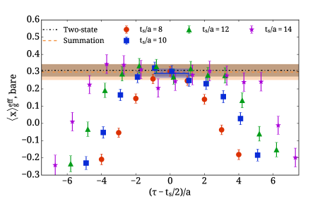
Figure 3: Results for the effective GMF from the B55.32 ensemble as a function of the insertion time-slice $\tau$ for four source-sink time separations. Red circles, blue squares, green triangles and magenta stars correspond to separations $t_{s}/a=8,\;10,\;12,\;14$, respectively. The blue band shows the extracted value using the plateau method with fit range specified by the band. Results from the two-state (summation) method are shown with grey (brown) band spanning the whole x-axis.

Figure 4: Extracted values for $\langle x\rangle_{g}^{\text{bare}}$ from B55.32 ensemble using the plateau, two-state and summation methods. The left column shows the extracted values from the plateau method varying the source-sink separation. The open red circle is the value we take as our final value. The right column shows the extracted values using the summation method (green triangles) and two-state fits (blue squares) as one varies the low fit range.

In order to study the excited state effects we compute the ratio of Eq. (11) for various source-sink time separations. In Fig. 3 we present the ratios from where we extract the matrix element using four separations as one varies the insertion time-slice using the B55.32 ensemble. We identify a window where excited states are sufficiently suppressed to perform a constant fit using the plateau method and we seek for convergence of this value to the ones extracted using the two-state and summation methods. Our findings are summarized in Fig. 4 where several fit ranges are analyzed. We take as our final value the one for the smallest $t_{s}$ which is compatible with the value extracted from the two-state method. The summation method usually has larger errors producing results compatible with the two-state method. Therefore, to be conservative we provide as a systematic error due to the excited states the difference between the plateau value and that extracted from the two-state fit.

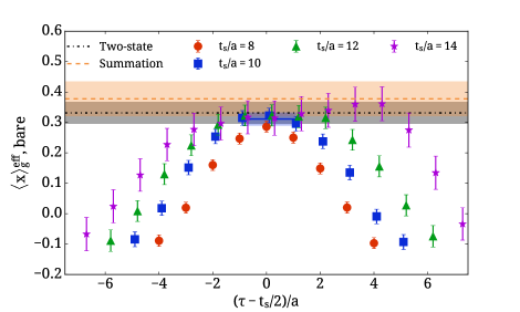
Figure 5: Results for the effective GMF from the cA2.09.48 ensemble. The notation is as in Fig.3.

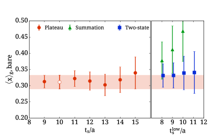
Figure 6: Extracted values for $\langle x\rangle_{g}^{\text{bare}}$ from the cA2.09.48 ensemble. The notation is as in Fig.4.

The results for the second ensemble with a physical value of the pion mass are presented in Figs. 5 - 6. In this case we applied 20 steps of stout smearing with $\omega{=}0.1315$. There is no evidence of a large influence of excited states within the statistics employed here. For the ensemble at the physical point, we extract the value of the GMF using the same procedure as the B55.32 ensemble. Our results are as follows:

$${\bf B55.32}: \,\,\langle x\rangle_{g}^{\text{bare}}=0.290(27)(17)\,,$$

$${\bf cA2.09.48}: \,\,\langle x\rangle_{g}^{\text{bare}}=0.311(22)(20)\,,$$ (17)

where the number in the first parenthesis is statistical, and the second is a systematic due to the excited states contamination. As mentioned above, the systematic uncertainty is the difference between the plateau method at $t_{s}/a{=}10$ and the two-state fit.

6 Renormalization - Final results

Yet another challenge regarding the computation of the physical value of the gluon momentum fraction is the fact that the lattice result has to be renormalized. Since the gluon operator is a flavor singlet operator, it will certainly mix with others, the quark singlet operator, for instance. In total, mixing with operators that are gauge invariant, Becchi-Rouet-Stora (BRS) variations, or vanish by the gluon equations of motion (e.o.m) [28] also appears. Due to this mixing appropriate renormalization conditions require computation of more than one matrix element, in order to extract the renormalization factors from a non-perturbative lattice calculation. This places additional difficulties compared to the renormalization procedure for other operators that are relevant for nucleon structure [29]. Consequently, a different approach has to be found, and in the framework of this paper we employ a one-loop perturbative renormalization procedure. In this section we briefly describe the setup of the calculation and final results needed to renormalize the GMF. Complete results will appear in a following publication [30].

The basis of operators that mix with each other (to one loop) is (see, e.g., [31])

$${\cal O}_{1}^{\mu\nu} = 2\,{\rm Tr}\left[G^{\{\mu\rho}G^{\nu\}\rho}\right]$$ (18)

$${\cal O}_{2}^{\mu\nu} = \bar{\psi}\,\gamma^{\{\mu}\,\mbox{\parbox[b]{0.0pt}{$D$}\raisebox{5.85553pt}{${\,\scriptstyle{\leftrightarrow}}$}}\,\phantom{}^{\nu\}}\psi$$ (19)

$${\cal O}_{3}^{\mu\nu} = \frac{1}{\alpha}\Big{[}\left(\partial^{\mu}A^{\nu}+\partial^{\nu}A^{\mu}\right)\left(\partial^{\rho}A^{\rho}\right)-\frac{1}{2}\delta_{\mu\nu}\left(\partial^{\rho}A^{\rho}\right)^{2}\Big{]}+{\rm ghost\,\,terms}$$ (20)

$${\cal O}_{4}^{\mu\nu} = \frac{1}{\alpha}\Big{[}-\left(\partial^{\mu}A^{\nu}+\partial^{\nu}A^{\mu}\right)\left(\partial^{\rho}A^{\rho}\right)-\frac{1}{2}\delta_{\mu\nu}A^{\rho}\partial^{\rho}\partial^{\sigma}A^{\sigma}\Big{]}+{\rm ghost\,\,terms}$$ (21)

$${\cal O}_{5}^{\mu\nu} = A^{\nu}\frac{\delta S}{\delta A^{\mu}}+A^{\mu}\frac{\delta S}{\delta A^{\nu}}-\frac{1}{2}\delta_{\mu\nu}\sum_{\rho}A^{\rho}\frac{\delta S}{\delta A^{\rho}}$$ (22)

where $\mbox{\parbox[b]{0.0pt}{$D$}\raisebox{5.85553pt}{${\,\scriptstyle{\leftrightarrow}}$}}=(\buildrel\rightarrow\over{D}\raise-1.0pt\hbox{}-\buildrel\leftarrow\over{D}\raise-1.0pt\hbox{})/2$. ${\cal O}^{\mu\nu}_{1}$ is the gluon operator under study, ${\cal O}^{\mu\nu}_{2}$ is the corresponding quark operator, ${\cal O}^{\mu\nu}_{3}$ and ${\cal O}^{\mu\nu}_{4}$ are BRS variation (they only differ by a total derivative) and ${\cal O}^{\mu\nu}_{5}$ vanishes by the equations of motion. The ghost parts of operators ${\cal O}^{\mu\nu}_{3}$ and ${\cal O}^{\mu\nu}_{4}$ are irrelevant for this one-loop computation and are not presented here. Note that in the calculation we employed traceless operators, and in such a case there are no lower dimensional two-index traceless symmetric tensors. Furthermore, we sum over the spatial position of the operator insertion, resulting in a momentum conservation when Fourier transforming in the momentum space. The external legs of the one-loop Feynman diagrams carry the same momentum.

From this point forward we concentrate on the singlet case, $\mu=\nu$, and we drop the Lorentz indices, that is, ${\cal O}_{i}\equiv{\cal O}_{i}^{\mu\mu}$ ($i=1,\cdots,5$). Furthermore, we indicate by ${\cal O}_{1}$ the combination resulting ${\cal O}_{B}$, in order to have the correct mixing coefficients. To identify and extract the multiplicative renormalization function of the gluon operator ${\cal O}_{1}$, one must construct a mixing matrix with elements that are appropriate Green’s functions of the above operators. However, mixing with ${\cal O}_{3}$ - ${\cal O}_{4}$ vanishes at the one-loop level and the matrix elements of the operator ${\cal O}_{5}$ between physical states vanish; the mixing matrix simplifies considerably. In particular, the only Feynman diagrams that enter our one-loop calculation are those of the operators ${\cal O}_{1}$ and ${\cal O}_{2}$, within external quarks and gluons. As we are interested in the renormalization of the operator ${\cal O}_{1}$ only, we present the relevant Feynman diagrams in Figs. 7 - 8.

Figure 7: One-loop Feynman diagrams contributing to the multiplicative renormalization of ${\cal O}_{1}$.

Figure 8: One-loop Feynman diagrams contributing to the mixing coefficient in ${\cal O}_{1}$ due to ${\cal O}_{2}$.

The most important consequence of the vanishing physical matrix elements of ${\cal O}_{3}$ - ${\cal O}_{5}$ is that the ratio shown in Eq. (8) is a linear combination of contributions from only ${\cal O}_{1}$ and ${\cal O}_{2}$. Note, however, that to correctly identify the multiplicative renormalization of ${\cal O}_{1}$, the operators ${\cal O}_{3}$ - ${\cal O}_{5}$ must be taken into account in the perturbative renormalization procedure (see Eq. (32)).

To make contact with phenomenological and experimental data, one needs the renormalization functions in the $\overline{\mathrm{MS}}$ scheme. An ideal method to extract the $\overline{\mathrm{MS}}$ results is to perform the computation in both dimensional (DR) and lattice (L) regularizations; one then extracts all relevant renormalization functions by demanding that renormalized lattice Green functions coincide with the corresponding ones in (DR), in the $a\to 0$ limit (cf. [32] for a similar application). Thus, one avoids intermediate schemes. Let us briefly outline this procedure below.

In cases of operator mixing, renormalized operators are related to the bare ones via $\hat{\cal O}^{R}=\hat{\cal Z}\,\hat{\cal O}$. In our case $\hat{\cal Z}$ is a $5\times 5$ mixing matrix of the form

$$\hat{\cal Z}=\hat{1}+{\cal O}(g^{2})\,,$$ (23)

where $g$ is the renormalized coupling constant. In this paper we are interested in the renormalization of the gluon operator, ${\cal O}_{1}$, and we only need to compute the first row of the mixing matrix to one-loop, which has only two non-zero matrix elements, that is $Z_{11}$ and $Z_{12}$. Alternatively, we write

$${\cal O}^{R}_{\alpha}=\sum_{\beta}Z_{\alpha\beta}{\cal O}_{\beta}\,\qquad\alpha,\beta=1,2\,.$$ (24)

In a more convenient notation, the $X$-$X$ bare amputated Green’s functions ($X=1(2)$: corresponds to a gluon(fermion) field) can be expressed in terms of the renormalized Green’s functions, that is,

$$\langle X{\cal O}_{\alpha}X\rangle=Z_{X}^{-1}\sum_{\beta}\left(Z^{-1}\right)_{\alpha\beta}\langle X{\cal O}_{\beta}X\rangle_{R}$$ (25)

where $Z_{X}$ is the renormalization function of the fermion/gluon field, defined via

$$\Psi=\sqrt{Z_{q}}\Psi^{R}\qquad A_{\nu}=\sqrt{Z_{A}}A_{\nu}^{R}$$ (26)

Dimensional Regularization

Next, we present the results in Dimensional Regularization for the amputated Green’s functions entering the renormalization of the gluon operator, ${\cal O}_{1}$. The renormalization functions in the $\overline{\mathrm{MS}}$ scheme in DR are defined such as to cancel the divergent parts of the matrix elements. The expressions related to the one-loop renormalization of the gluon operator reduce to

$$\Lambda_{11}^{\mathrm{1-loop}}\Bigg{|}_{1/\epsilon} = \left(-z_{A}-z_{11}\right)\Lambda_{11}^{\mathrm{tree}}-z_{31}\Lambda_{31}^{\mathrm{tree}}-z_{41}\Lambda_{41}^{\mathrm{tree}}-z_{51}\Lambda_{51}^{\mathrm{tree}}$$ (27)

$$\Lambda_{12}^{\mathrm{1-loop}}\Bigg{|}_{1/\epsilon} = -z_{12}\Lambda_{12}^{\mathrm{tree}}$$ (28)

where $\Lambda_{aX}\equiv\langle X{\cal O}_{\alpha}X\rangle$ and $z$’s are the one-loop contributions of the corresponding renormalization functions, that is

$$Z_{A}=1+z_{A}+{\cal O}(g^{4})$$ (29)

$$Z_{ii}=1+z_{ii}+{\cal O}(g^{4})$$ (30)

$$Z_{ij}=0+z_{ij}+{\cal O}(g^{4})$$ (31)

It should be noted that, modulo a total derivative, the gluon parts of ${\cal O}_{3}$ and ${\cal O}_{4}$ coincide ($\Lambda^{\rm tree}_{31}=\Lambda^{\rm tree}_{41}$) and, thus, we cannot disentangle $z_{31}$ and $z_{41}$ from the Green’s functions we study. However, this does not affect the extraction of $z_{11}$.

In our one-loop calculation we find:

$$\Lambda_{11}^{\mathrm{1-loop,DR}}\Bigg{|}_{1/\epsilon} = \frac{g^{2}}{16\,\pi^{2}}\frac{N_{c}}{\epsilon}\Bigg{[}\Lambda_{11}^{\mathrm{tree,DR}}\left(-\frac{5}{3}-\frac{\beta}{2}\right)$$ (32)

$$\hskip 28.45274pt-\left(\Lambda_{31}^{\mathrm{tree,DR}}+\Lambda_{41}^{\mathrm{tree,DR}}\right)-2\,\Lambda_{51}^{\mathrm{tree,DR}}\Bigg{]}$$

$$\Lambda_{12}^{\mathrm{1-loop,DR}}\Bigg{|}_{1/\epsilon} = \frac{g^{2}}{16\,\pi^{2}}\frac{N_{c}^{2}-1}{\epsilon\,N_{c}}\,\Lambda_{22}^{\mathrm{tree,DR}}\left(\frac{5}{3}+\beta\right)$$ (33)

By definition, the finite terms of $\Lambda_{ij}^{\mathrm{1-loop,DR}}$ do not appear in the evaluation of $Z_{ij}^{\mathrm{1-loop,DR}}$, but they are key elements in obtaining $Z_{ij}^{\mathrm{L,\overline{\mathrm{MS}}}}$ as explained below.

Let us slightly modify our notation and use the gluon and quark momentum fraction of the nucleon, $\langle x\rangle_{g}$ and $\langle x\rangle_{q}$, which are more relevant for this paper. For demonstration purposes we will represent the mixing of physical matrix elements as a $2\times 2$ matrix

$$\binom{\langle x\rangle_{g}}{\sum_{q}\langle x\rangle_{q}}=\begin{pmatrix}Z_{11}&Z_{12}\\ Z_{21}&Z_{22}\end{pmatrix}\binom{\langle x\rangle_{g}^{\text{bare}}}{\sum_{q}\langle x\rangle_{q}^{\text{bare}}}\,.$$ (34)

Thus, the physical result of the gluon momentum fraction can be related to the non-perturbative results for $\langle x\rangle_{g}$ and $\langle x\rangle_{q}$ by

$$\langle x\rangle_{g}^{R}=Z_{11}\langle x\rangle_{g}+Z_{12}\sum_{q}\langle x\rangle_{q}\,,$$ (35)

where a certain scheme, e.g. $\overline{\mathrm{MS}}$, and an energy scale $\mu$ have to be chosen. The expressions for $Z_{11}$ and $Z_{12}$ in DR and in the $\overline{\mathrm{MS}}$ scheme are

$$Z_{11}=1+\frac{g^{2}\,N_{f}}{16\,\pi^{2}}\frac{2}{3\,\epsilon}$$ (36)

$$Z_{12}=0-\frac{g^{2}\,C_{f}}{16\,\pi^{2}}\frac{8}{3\,\epsilon}$$ (37)

where $C_{f}=\frac{N_{c}^{2}-1}{2N_{c}}$.

Lattice Regularization

To obtain the corresponding lattice results for $Z_{ij}$ in the $\overline{\mathrm{MS}}$ scheme we will make use of the DR results, so that an indermediate Regularization independend (RI) type prescription is avoided. Renormalizability of the theory implies that the difference between the one-loop renormalized and bare Green’s functions is polynomial in the external momentum (of degree 0, in our case, since no lower-dimensional operators mix); this results in an appropriate definition of the momentum-independent renormalization functions $Z_{ij}^{\mathrm{L,\overline{\mathrm{MS}}}}$. More precisely, for the operators under study we find to one loop

$$\langle A_{\nu}{\cal O}_{1}A_{\nu}\rangle^{\mathrm{DR,\overline{\mathrm{MS}}}}-\langle A_{\nu}{\cal O}_{1}A_{\nu}\rangle^{\mathrm{L}} = \left(z_{A}^{\mathrm{L,\overline{\mathrm{MS}}}}+z_{11}^{\mathrm{L,\overline{\mathrm{MS}}}}\right)\,\Lambda^{\mathrm{tree}}_{11}$$ (38)

$$+ \left(z_{31}^{\mathrm{L,\overline{\mathrm{MS}}}}+z_{41}^{\mathrm{L,\overline{\mathrm{MS}}}}\right)\,\Lambda^{\mathrm{tree}}_{31}+z_{51}^{\mathrm{L,\overline{\mathrm{MS}}}}\,\Lambda^{\mathrm{tree}}_{51}\,\,\,\,\,$$

$$\langle\Psi{\cal O}_{1}\Psi\rangle^{\mathrm{DR,\overline{\mathrm{MS}}}}-\langle\Psi{\cal O}_{1}\Psi\rangle^{\mathrm{L}} = z_{12}^{\mathrm{L,\overline{\mathrm{MS}}}}\,\Lambda^{\mathrm{tree}}_{22}$$ (39)

It should be noted that the smearing of the operator modifies its renormalization factor, and thus for a proper renormalization it is required to apply the same smearing in the perturbative calculation. The main technical difficulty in such a case is that the smearing leads to extremely lengthy expressions for the operator’s vertices. For example, the 4-gluon vertex for two smearing steps with general smearing parameters, $\omega_{1}$ and $\omega_{2}$, contains approximately 335,000 terms. This places severe limitations on the number of smearing iterations we can apply to the operator. In our computation we extract the vertices with up to two stout smearing steps with distinct parameters. This allows us to compare values of the renormalization functions for the single- and double-smeared operator. We find that increasing the number of smearing steps has small effect on the renormalization functions. This is due to a combination of the small value of the smearing parameter and the polynomial dependence on $\omega_{1}$ and $\omega_{2}$. We also note that the perturbative calculation is performed for general action parameters, so that the results are applicable for a variety of gluon/fermion actions.

The general expressions for $Z_{11}$ and $Z_{12}$ are complicated $4^{\rm th}$-degree polynomials of $\omega_{1}$ and $\omega_{2}$, and cannot be presented here. Thus, we write them in a compact form, as a function of the quantities $e^{(i)}_{11/12}\equiv e^{(i)}_{11/12}(\omega_{1},\omega_{2})$, which also depend on the gluon action parameters

$$Z^{\mathrm{L,\overline{\mathrm{MS}}}}_{11} = 1+\frac{g^{2}}{16\pi^{2}}\left(\frac{e^{(1)}_{11}}{N_{c}}+e^{(2)}_{11}\,N_{f}-\frac{2\,N_{f}}{3}\log(a^{2}\bar{\mu}^{2})\right)$$ (40)

$$Z^{\mathrm{L,\overline{\mathrm{MS}}}}_{12} = 0+\frac{g^{2}\,C_{f}}{16\pi^{2}}\left(e^{(1)}_{12}+e^{(2)}_{12}\,c_{\rm SW}+\frac{8}{3}\log(a^{2}\bar{\mu}^{2})\right)\,.$$ (41)

The computation of the quantities $e^{(i)}_{11/12}$ is the most laborious part of the perturbative work and required the equivalent of approximately 40 years of computation on a single CPU. This includes, among other parts, the integration of the internal loop momentum for several lattice sizes and the extrapolation to the infinite volume limit. The numerical results for the multiplicative renormalization function, $Z_{11}^{\overline{\mathrm{MS}}}$ and the mixing coefficient, $Z_{12}^{\overline{\mathrm{MS}}}$, are given in Table 2 in the $\overline{\mathrm{MS}}$ scheme at a scale of $2\,\mathrm{GeV}$. The statistical errors associated with the infinite volume extrapolation are smaller than the accuracy presented in the table. One can observe that the effect of additional smearing steps tends to become suppressed. This is due to the polynomial dependence on $\omega_{1}$ and $\omega_{2}$, combined with the fact that their numerical value is very small. It is expected that the effect of further smearing steps will be smaller than the difference between the 1- and 2-stout results shown in Table 2. Thus, we employ the renormalization factors using the 2-stout results to renormalize the matrix element presented in Section 5.

		$Z_{11}^{\mathrm{L,\overline{\mathrm{MS}}}}$			$Z_{12}^{\mathrm{L,\overline{\mathrm{MS}}}}$
	0-stout	1-stout	2-stout	0-stout	1-stout	2-stout
B55.32	0.9481	1.0043	1.0134	0.1720	0.0278	-0.0168
cA2.09.48	0.8985	0.9506	0.9590	0.1120	-0.0070	-0.0436

Table 2: Multiplicative renormalization and mixing coefficient for the gluon operator. Results are given in the $\overline{\mathrm{MS}}$ scheme at a scale of $2\,\mathrm{GeV}$.

According to Eq. (35) the bare quark momentum fraction enters the renormalization prescription of the gluon momentum fraction. The quark contributions have been computed for both the connected and disconnected diagrams for B55.32 [25, 3] and cA2.09.48 [5, 33, 34]. Using the bare results

$${\bf B55.32}: \,\,\langle x\rangle_{u+d}=0.603(79)$$

$${\bf cA2.09.48}: \,\,\langle x\rangle_{u+d+s}=0.722(96)\,,$$ (42)

we find the following values for the renormalized gluon momentum fraction in the $\overline{\mathrm{MS}}$ at $\mu=2\,\mathrm{GeV}$:

$${\rm{\bf B55.32}}: \,\,\langle x\rangle^{R}_{g}=0.284(27)(17)(24)$$

$${\rm{\bf cA2.09.48}}: \,\,\langle x\rangle^{R}_{g}=0.267(22)(19)(24)\,.$$ (43)

The numbers in the first parenthesis correspond to the statistical error, the second is a systematic due to the excited states, and the third one is systematic taken as the difference between the single- and double- smeared results; this is within the statistical errors.

Taking into account the disconnected quark contribution has small effect on $\langle x\rangle^{R}_{g}$ due to the mild mixing when stout smearing is applied on the gluon operator. Complete results on the quark and gluon momentum fraction appear in Ref. [35].

7 Conclusion and outlook

In this paper we applied the direct method to compute the average momentum fraction of the gluon in the nucleon, $\langle x\rangle_{g}$, taking into account the mixing with the singlet, light quark contribution. In order to obtain statistically significant results for the involved, purely disconnected 3-point functions, several steps of stout smearing to the gauge links that enter the operator were employed. Nevertheless, a substantial amount of measurements was needed to obtain a good signal with about 10% statistical error.

We computed the average momentum fraction for two gauge field ensembles. The first has $N_{f}{=}2{+}1{+}1$ flavors representing the first two quark generations at a pion mass of about 370 MeV with 34470 measurements. The second ensemble has $N_{f}{=}2$ mass degenerate up and down quarks at the physical value of the pion mass, with 204900 measurements. The number of measurements for the two cases allowed us to obtain statistically significant values for the bare matrix elements (see Eq. (17)).

Since the required gluon operator is a singlet operator, it mixes with the corresponding singlet quark operator. As a consequence, the renormalization of the gluon operator is highly non-trivial since this mixing has to be taken into account. To this end, we have performed a perturbative calculation for the mixing and the renormalization. This has been done in the dimensional and the lattice regularizations. Moreover, the stout smearing that we employed in the lattice computation of the bare matrix element had to be taken into account in the perturbative calculation. This led to a very complicated perturbative calculation which involved several diagrams with $\mathcal{O}(100000)$ intermediate expressions. Still, we could demonstrate that with the inclusion of two stout smearing levels a saturation of the renormalization functions could be observed. The renormalization functions obtained in this manner have been used for the renormalization of gluon and the corresponding singlet quark moments. The final results for the renormalized gluon momentum fraction are summarized in Eq. (43), and in Ref. [35] for the quark singlet quantities. The values can serve for a comparison with a phenomenological extraction of these quantities from deep inelastic scattering experiments. Our results also demonstrate that the gluon indeed contributes a significant amount of the momentum fraction of about 30%.

Our calculations can be extended to evaluate the spin content of the nucleon, a topic we would like to report on in the future. In addition, the renormalization functions computed here can directly be used for the renormalization of the corresponding average fractional momenta of the pion.

References

- [1] C. Alexandrou, “Nucleon structure from lattice QCD - recent achievements and perspectives,” EPJ Web Conf. 73 (2014) 01013, arXiv:1404.5213 [hep-lat].
- [2] M. Constantinou, “Hadron Structure,” PoS LATTICE2014 (2014) 001, arXiv:1411.0078 [hep-lat].
- [3] A. Abdel-Rehim, C. Alexandrou, M. Constantinou, V. Drach, K. Hadjiyiannakou, K. Jansen, G. Koutsou, and A. Vaquero, “Disconnected quark loop contributions to nucleon observables in lattice QCD,” Phys. Rev. D89 no. 3, (2014) 034501, arXiv:1310.6339 [hep-lat].
- [4] C. Alexandrou, M. Constantinou, V. Drach, K. Hadjiyiannakou, K. Jansen, et al., “Evaluation of disconnected quark loops for hadron structure using GPUs,” Comput.Phys.Commun. 185 (2014) 1370–1382, arXiv:1309.2256 [hep-lat].
- [5] A. Abdel-Rehim et al., “Nucleon and pion structure with lattice QCD simulations at physical value of the pion mass,” Phys. Rev. D92 no. 11, (2015) 114513, arXiv:1507.04936 [hep-lat]. [Erratum: Phys. Rev. D93 no. 3, (2016) 039904].
- [6] X. Xiong, X. Ji, J.-H. Zhang, and Y. Zhao, “One-loop matching for parton distributions: Nonsinglet case,” Phys. Rev. D90 no. 1, (2014) 014051, arXiv:1310.7471 [hep-ph].
- [7] H.-W. Lin, J.-W. Chen, S. D. Cohen, and X. Ji, “Flavor Structure of the Nucleon Sea from Lattice QCD,” Phys. Rev. D91 (2015) 054510, arXiv:1402.1462 [hep-ph].
- [8] C. Alexandrou, K. Cichy, V. Drach, E. Garcia-Ramos, K. Hadjiyiannakou, K. Jansen, F. Steffens, and C. Wiese, “Lattice calculation of parton distributions,” Phys. Rev. D92 no. 1, (2015) 014502, arXiv:1504.07455 [hep-lat].
- [9] Y.-B. Yang, R. S. Sufian, A. Alexandru, T. Draper, M. J. Glatzmaier, K.-F. Liu, and Y. Zhao, “Glue Spin and Helicity in the Proton from Lattice QCD,” Phys. Rev. Lett. 118 no. 10, (2017) 102001, arXiv:1609.05937 [hep-ph].
- [10] M. Gockeler, R. Horsley, E.-M. Ilgenfritz, H. Oelrich, H. Perlt, P. E. L. Rakow, G. Schierholz, A. Schiller, and P. Stephenson, “A Preliminary lattice study of the glue in the nucleon,” Nucl. Phys. Proc. Suppl. 53 (1997) 324–326, arXiv:hep-lat/9608017 [hep-lat].
- [11] QCDSF, UKQCD Collaboration, R. Horsley et al., “A Lattice Study of the Glue in the Nucleon,” Phys. Lett. B714 (2012) 312–316, arXiv:1205.6410 [hep-lat].
- [12] K. F. Liu et al., “Quark and Glue Momenta and Angular Momenta in the Proton — a Lattice Calculation,” PoS LATTICE2011 (2011) 164, arXiv:1203.6388 [hep-ph].
- [13] M. Deka et al., “Lattice study of quark and glue momenta and angular momenta in the nucleon,” Phys. Rev. D91 no. 1, (2015) 014505, arXiv:1312.4816 [hep-lat].
- [14] S. Alekhin, J. Blumlein, and S. Moch, “The ABM parton distributions tuned to LHC data,” Phys. Rev. D89 no. 5, (2014) 054028, arXiv:1310.3059 [hep-ph].
- [15] R. Frezzotti and G. Rossi, “Chirally improving Wilson fermions. 1. O(a) improvement,” JHEP 0408 (2004) 007, arXiv:hep-lat/0306014 [hep-lat].
- [16] R. Frezzotti and G. C. Rossi, “Chirally improving Wilson fermions. II. Four-quark operators,” JHEP 10 (2004) 070, arXiv:hep-lat/0407002 [hep-lat].
- [17] H. B. Meyer and J. W. Negele, “Gluon contributions to the pion mass and light cone momentum fraction,” Phys. Rev. D77 (2008) 037501, arXiv:0707.3225 [hep-lat].
- [18] C. Alexandrou, V. Drach, K. Hadjiyiannakou, K. Jansen, B. Kostrzewa, and C. Wiese, “Looking at the gluon moment of the nucleon with dynamical twisted mass fermions,” PoS LATTICE2013 (2014) 289, arXiv:1311.3174 [hep-lat].
- [19] X.-D. Ji, “A QCD analysis of the mass structure of the nucleon,” Phys. Rev. Lett. 74 (1995) 1071–1074, arXiv:hep-ph/9410274 [hep-ph].
- [20] C. Best, M. Gockeler, R. Horsley, E.-M. Ilgenfritz, H. Perlt, P. E. L. Rakow, A. Schafer, G. Schierholz, A. Schiller, and S. Schramm, “Pion and rho structure functions from lattice QCD,” Phys. Rev. D56 (1997) 2743–2754, arXiv:hep-lat/9703014 [hep-lat].
- [21] Zeuthen-Rome (ZeRo) Collaboration, M. Guagnelli, K. Jansen, F. Palombi, R. Petronzio, A. Shindler, and I. Wetzorke, “Non-perturbative pion matrix element of a twist-2 operator from the lattice,” Eur. Phys. J. C40 (2005) 69–80, arXiv:hep-lat/0405027 [hep-lat].
- [22] R. Baron et al., “Light hadrons from lattice QCD with light (u,d), strange and charm dynamical quarks,” JHEP 1006 (2010) 111, arXiv:1004.5284 [hep-lat].
- [23] C. Alexandrou, V. Drach, K. Jansen, C. Kallidonis, and G. Koutsou, “Baryon spectrum with twisted mass fermions,” Phys. Rev. D90 no. 7, (2014) 074501, arXiv:1406.4310 [hep-lat].
- [24] ETM Collaboration, A. Abdel-Rehim et al., “First physics results at the physical pion mass from Wilson twisted mass fermions at maximal twist,” Phys. Rev. D95 no. 9, (2017) 094515, arXiv:1507.05068 [hep-lat].
- [25] C. Alexandrou, M. Constantinou, S. Dinter, V. Drach, K. Jansen, et al., “Nucleon form factors and moments of generalized parton distributions using twisted mass fermions,” Phys. Rev. D88 no. 1, (2013) 014509, arXiv:1303.5979 [hep-lat].
- [26] A. Hasenfratz and F. Knechtli, “Flavor symmetry and the static potential with hypercubic blocking,” Phys. Rev. D64 (2001) 034504, arXiv:hep-lat/0103029 [hep-lat].
- [27] C. Morningstar and M. J. Peardon, “Analytic smearing of SU(3) link variables in lattice QCD,” Phys. Rev. D69 (2004) 054501, arXiv:hep-lat/0311018 [hep-lat].
- [28] S. Joglekar and B. Lee, “General Theory of Renormalization of Gauge Invariant Operators,” Ann.Phys. 97 (1976) 160.
- [29] C. Alexandrou, M. Constantinou, T. Korzec, H. Panagopoulos, and F. Stylianou, “Renormalization constants for 2-twist operators in twisted mass QCD,” Phys. Rev. D83 (2011) 014503, arXiv:1006.1920 [hep-lat].
- [30] M. Constantinou and H. Panagopoulos. In preparation.
- [31] S. Caracciolo, P. Menotti, and A. Pelissetto, “One loop analytic computation of the energy momentum tensor for lattice gauge theories,” Nucl. Phys. B375 (1992) 195–239.
- [32] M. Constantinou, M. Costa, R. Frezzotti, V. Lubicz, G. Martinelli, D. Meloni, H. Panagopoulos, and S. Simula, “Renormalization of the chromomagnetic operator on the lattice,” Phys. Rev. D92 no. 3, (2015) 034505, arXiv:1506.00361 [hep-lat].
- [33] C. Alexandrou, M. Constantinou, K. Hadjiyiannakou, C. Kallidonis, G. Koutsou, K. Jansen, C. Wiese, and A. V. Aviles-Casco, “Nucleon spin and quark content at the physical point,” PoS LATTICE2016 (2016) 153, arXiv:1611.09163 [hep-lat].
- [34] A. Abdel-Rehim, C. Alexandrou, M. Constantinou, J. Finkenrath, K. Hadjiyiannakou, K. Jansen, C. Kallidonis, G. Koutsou, A. V. Aviles-Casco, and J. Volmer, “Disconnected diagrams with twisted-mass fermions,” PoS LATTICE2016 (2016) 155, arXiv:1611.03802 [hep-lat].
- [35] C. Alexandrou, M. Constantinou, K. Hadjiyiannakou, K. Jansen, C. Kallidonis, G. Koutsou, A. V. Aviles-Casco, and C. Wiese, “Nucleon spin and momentum decomposition using lattice QCD simulations,” accepted in Phys. Rev. Lett. (2017) , arXiv:1706.02973 [hep-lat].