Bidirectional Tree-Structured LSTM with Head Lexicalization

Abstract

Sequential LSTM has been extended to model tree structures, giving competitive results for a number of tasks. Existing methods model constituent trees by bottom-up combinations of constituent nodes, making direct use of input word information only for leaf nodes. This is different from sequential LSTMs, which contain reference to input words for each node. In this paper, we propose a method for automatic head-lexicalization for tree-structure LSTMs, propagating head words from leaf nodes to every constituent node. In addition, enabled by head lexicalization, we build a tree LSTM in the top-down direction, which corresponds to bidirectional sequential LSTM structurally. Experiments show that both extensions give better representations of tree structures. Our final model gives the best results on the Standford Sentiment Treebank and highly competitive results on the TREC question type classification task.

1 Introduction

Both sequence structured and tree structured neural models have been applied to NLP problems. Seminal work employs convolutional neural network [Collobert and Weston, 2008], recurrent neural network [Elman, 1990, Mikolov et al., 2010] and recursive neural network [Socher et al., 2011] for sequence and tree modeling. Recently, Long Short-Term Memories (LSTM) have received increasing research attention, giving significantly improved accuracies in a variety of sequence tasks [Sutskever et al., 2014, Bahdanau et al., 2014] compared to vanilla recurrent neural networks. Addressing diminishing gradients effectively, they have been extended to tree structures, achieving promising results for tasks such as syntactic language modeling [Zhang et al., 2015], sentiment analysis [Li et al., 2015, Zhu et al., 2015b, Le and Zuidema, 2015, Tai et al., 2015] and relation extraction [Miwa and Bansal, 2016].

According to the node type, typical tree structures in NLP can be categorized to constituent trees and dependency trees. A salient difference between the two types of tree structures is in the node. While dependency tree nodes are input words themselves, constituent tree nodes represent syntactic constituents. Only leaf nodes in constituent trees correspond to words. Though LSTM structures have been developed for both types of trees above, we investigate constituent trees in this paper. There are three existing methods for constituent tree LSTM [Zhu et al., 2015b, Tai et al., 2015, Le and Zuidema, 2015], which make essentially the same extension from sequence structure LSTMs. We take the method of ?) as our baseline.

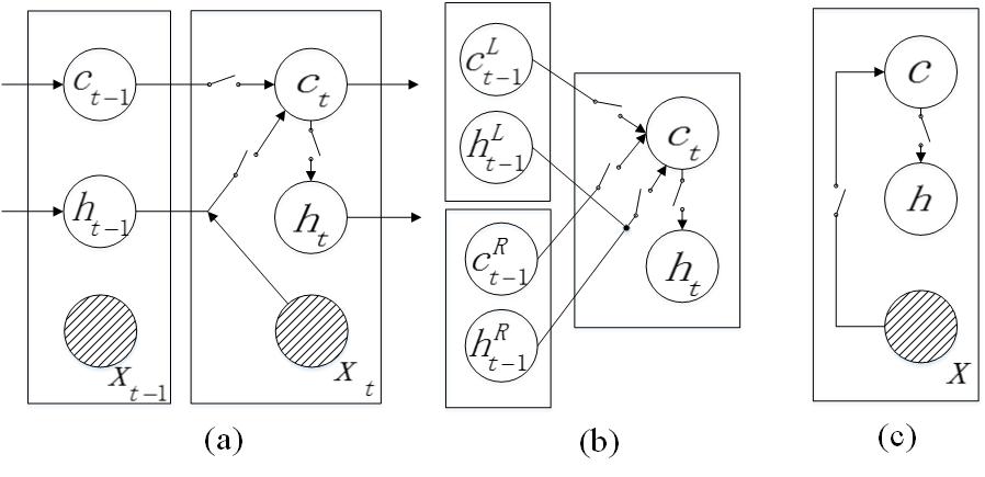
Figure 1: Topology of sequential and tree LSTMs. (a) nodes in sequential LSTM; (b) non-leaf nodes in tree LSTM; (c) leaf nodes in tree LSTM. Shaded nodes represent lexical input vectors. White nodes represent hidden state vectors.

A contrast between the sequence structured LSTM of ?) and the tree-structured LSTM of ?) is shown in Figure 1, which illustrates the input ($x$), cell ($c$) and hidden ($h$) nodes at a certain time step $t$. The most important difference between Figure 1(a) and Figure 1(b) is the branching factor. While a cell in the sequence structure LSTM depends on the single previous hidden node, a cell in the tree-structured LSTM depends on a left hidden node and a right hidden node. Such tree-structured extension of the sequence structure LSTM assumes that the constituent tree is binarized, building hidden nodes from the input words in the bottom-up direction. The leaf node structure in shown in Figure 1(c).

A second salient difference between the two types of LSTMs is the modeling of input words. While each cell in the sequence structure LSTM directly depends on its corresponding input word, only leaf cells in the tree structure LSTM directly depend on corresponding input words. This corresponds well to the constituent tree structure, where there is no direct association between non-leaf constituent nodes and input words. However, it leaves the tree structure a degraded version of a perfect binary-branching variation of the sequence-structure LSTM, with one important source of information (i.e. words) missing in forming a cell.

We fill this gap by proposing an extension to the tree LSTM model, injecting lexical information into every node in the tree. Our method takes inspiration from work on head-lexicalization, which shows that each node in a constituent tree structure is governed by a head word. As shown in Figure 2, the head word for the verb phrase “visited Mary” is “visited”, and the head word of the adverb phrase “this afternoon” is “afternoon”. Research has shown that head word information can significantly improve the performance of syntactic parsing [Collins, 2003, Clark and Curran, 2004]. Correspondingly, we use head lexical information of each constituent word as the input node $x$ for calculating the corresponding cell $c$ in Figure 1(b).

Traditional head-lexicalization relies on specific rules [Collins, 2003], typically extracting heads from constituent treebanks according to certain grammar formalisms. For better generalization, we use a neural attention mechanism to derive head lexical information automatically, rather than relying on linguistic head rules to find the head lexicon of each constituent, which is language- and formalism-dependent.

Based on such head lexicalization, we make a bidirectional extension of the tree structured LSTM, propagating information in the top-down direction as well as the bottom-up direction. This is analogous to the bidirectional extension of sequence structure LSTMs, which are commonly used for NLP tasks such as speech recognition [Graves et al., 2013], sentiment analysis [Tai et al., 2015, Li et al., 2015] and machine translation [Sutskever et al., 2014, Bahdanau et al., 2014] tasks.

Results on a standard sentiment classification benchmark and a question type classification benchmark show that our tree LSTM structure gives significantly better accuracies compared with the method of ?). We achieve the best reported results for sentiment classification. Interestingly, the head lexical information that is learned automatically from the sentiment treebank consists of both syntactic head information and key sentiment word information. This shows the advantage of automatic head-finding as compared with rule-based head lexicalization. We make our code available under GPL at https://github.com/XXX/XXX.

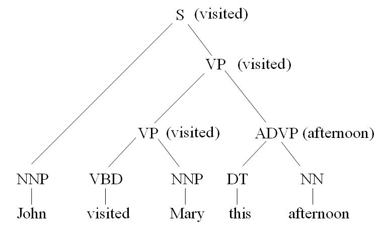
Figure 2: Head-Lexicalized Constituent Tree.

2 Related Work

LSTM [Hochreiter and Schmidhuber, 1997] is a variation of RNN [Elman, 1990] to solve vanishing gradients in training. It has been widely adopted for NLP tasks, such as parsing [Dyer et al., 2015] and machine translation [Bahdanau et al., 2014]. We take the standard LSTM with peephole connections [Gers and Schmidhuber, 2000] as our baseline, which models sequences.

There has been extensions of sequence-structured LSTMs for modeling trees [Tai et al., 2015, Le and Zuidema, 2015, Zhu et al., 2015b]. The idea is similar to extending recursive neural network to recurrent neural network, where gates are used in recursive structures for alleviating diminishing gradients. While ?) investigated tree-structured LSTMs for both dependency structures and constituent structures, and both for unrestricted trees and M-nary trees, ?) and ?) focused on binary constituent trees. As discussed earlier, none of these existing methods make direct use of lexical input for composing constituent vectors. We take ?) as our baseline.

Bidirectional information has been leveraged to extend sequence LSTM [Graves et al., 2013]. On the other hand, the aforementioned tree-LSTM models work bottom-up, without information flew from parents to children. ?) built a top-down tree-LSTM for dependency trees, but without a bottom-up component. ?) made use of bidirectional information on binary trees, but for recursive neural networks only. The closest in spirit to our method, ?) adopted a bidirectional Tree LSTM model to jointly extract named entities and relations under dependency tree structure. For constituent tree structures, however, their model does not work due to lack of word inputs on non-leaf constituent nodes, and in particular the root node. Our head lexicalization allows us to investigate the top-down constituent Tree LSTM. To our knowledge, we are the first to report a bidirectional constituent Tree LSTM.

3 Baselines

A sequence-structure LSTM estimates a sequence of hidden state vectors given a sequence of input vectors, through the calculation of a sequence of hidden cell vectors using a gate mechanism. For NLP, the input vectors are typically word embeddings [Mikolov et al., 2013], but can also include PoS embeddings, character embeddings or other types of information. For notational convenience, we refer to the input vectors as lexical vectors.

Formally, given an input vector sequence $x_{1},x_{2},\dots,x_{n}$, each state vector $h_{t}$ is estimated from the Hadamard product of a cell vector $c_{t}$ and a corresponding output gate vector $o_{t}$

$$h_{t}=o_{t}\otimes\tanh(c_{t})$$ (1)

Here the cell vector depends on both the previous cell vector $c_{t}$, and a combination of the previous state vector $h_{t-1}$, the current input vector $x_{t}$:

$$c_{t}=f_{t}\otimes c_{t-1}+i_{t}\otimes g_{t}$$ (2)

$$g_{t}=\tanh(W_{xg}x_{t}+W_{hg}h_{t-1}+b_{g})$$ (3)

The combination of $c_{t-1}$ and $g_{t}$ are controlled by the Hadamard product between a forget gate vector $f_{t}$ and a input gate vector $i_{t}$, respectively. The gates $o_{t}$, $f_{t}$ and $i_{t}$ are defined as follows

$$\begin{split}i_{t}&=\sigma(W_{xi}x_{t}+W_{hi}h_{t-1}+W_{ci}c_{t-1}+b_{i})\\ f_{t}&=\sigma(W_{xf}x_{t}+W_{hf}h_{t-1}+W_{cf}c_{t-1}+b_{f})\\ o_{t}&=\sigma(W_{xo}x_{t}+W_{ho}h_{t-1}+W_{co}c_{t}+b_{o}),\\ \end{split}$$ (4)

where $\sigma$ is the sigmoid function. $W_{xg}$, $W_{hg}$, $b_{g}$, $W_{xi}$, $W_{hi}$, $W_{ci}$, $b_{i}$, $W_{xf}$, $W_{hf}$, $W_{cf}$, $b_{f}$, $W_{xo}$, $W_{ho}$, $W_{co}$ and $b_{o}$ are model parameters.

The bottom-up Tree LSTM of ?) extends the left-to-right sequence LSTM by splitting the previous state vector $h_{t-1}$ into a left child state vector $h_{t-1}^{L}$ and a right child state vector $h_{t-1}^{R}$, and the previous cell vector $c_{t-1}$ into a left child cell vector $c_{t-1}^{L}$ and a right child cell vector $c_{t-1}^{R}$, calculating $c_{t}$ as

$$c_{t}=f_{t}^{L}\otimes c_{t-1}^{L}+f_{t}^{R}\otimes c_{t-1}^{R}+i_{t}\otimes g_{t},$$ (5)

and the input/output gates $i_{t}$/$o_{t}$ as

$$\begin{split}i_{t}&=\sigma\Big{(}\sum_{N\in\{L,R\}}(W_{hi}^{N}h_{t-1}^{N}+W_{ci}^{N}c_{t-1}^{N})+b_{i}\Big{)}\\ o_{t}&=\sigma\Big{(}\sum_{N\in\{L,R\}}W_{ho}^{N}h_{t-1}^{N}+W_{co}c_{t}+b_{o}\Big{)}\\ \end{split}$$ (6)

The forget gate $f_{t}$ is split into $f_{t}^{L}$ and $f_{t}^{R}$ for regulating $c_{t-1}^{L}$ and $c_{t-1}^{R}$, respectively:

$$\begin{split}f_{t}^{L}&=\sigma\Big{(}\sum_{N\in\{L,R\}}(W_{hf_{l}}^{N}h_{t-1}^{N}+W_{cf_{l}}^{N}c_{t-1}^{N})+b_{f_{l}}\Big{)}\\ f_{t}^{R}&=\sigma\Big{(}\sum_{N\in\{L,R\}}(W_{hf_{r}}^{N}h_{t-1}^{N}+W_{cf_{r}}^{N}c_{t-1}^{N})+b_{f_{r}}\Big{)}\\ \end{split}$$ (7)

$g_{t}$ depends on both $h_{t-1}^{L}$ and $h_{t-1}^{R}$, but as shown in Figure 1 (b), it does not depend on $x_{t}$

$$g_{t}=\tanh\Big{(}\sum_{N\in\{L,R\}}W_{hg}^{N}h_{t-1}^{N}+b_{g}\Big{)}$$ (8)

Finally, the hidden state vector $h_{t}$ is calculated in the same way as in the sequential LSTM model shown in Equation 1. $W_{hi}^{L}$, $W_{hi}^{R}$, $W_{ci}^{L}$, $W_{ci}^{R}$, $b_{i}$, $W_{ho}^{L}$, $W_{ho}^{R}$, $W_{co}$, $b_{o}$, $W_{hf_{l}}^{L}$, $W_{hf_{l}}^{R}$, $W_{cf_{l}}^{L}$, $W_{cf_{l}}^{R}$, $b_{f_{l}}$, $W_{hf_{r}}^{L}$, $W_{hf_{r}}^{R}$, $W_{cf_{r}}^{L}$, $W_{cf_{r}}^{R}$, $b_{f_{r}}$, $W_{hg}^{L}$, $W_{hg}^{R}$ and $b_{g}$ are model parameters.

4 Our Model

4.1 Head Lexicalization

We introduce an input lexical vector $x_{t}$ to the calculation of each cell vector $c_{t}$ via a bottom-up head propagation mechanism. As shown in the shaded nodes in Figure 3 (b), the head propagation mechanism stands relatively in parallel to the cell propagation mechanism. In contrast, the method of ?) in Figure 3 (a) does not have the input vector $x_{t}$ for non-leaf constituents.

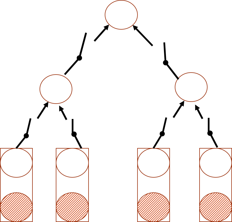
(a)

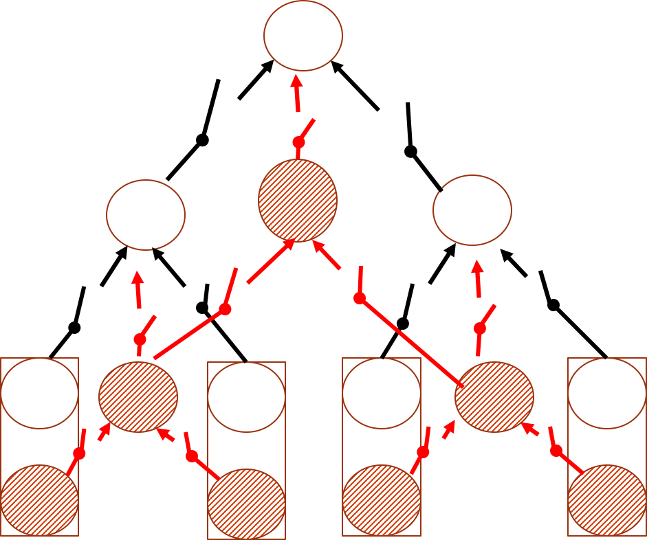
(b)

Figure 3: Contrast between ?) (a) and this paper (b). Shaded nodes represent lexical input vectors. White nodes represent hidden state vectors.

There are multiple ways to choose a head lexicon for a given binary-branching constituent. One simple baseline is to choose the head lexicon of the left child as the head (left-headedness). Correspondingly, an alternative is to use the right child for head lexicon. However, these simple baselines can bring less benefits compared to linguistically motivated head finding, due to relatively less consistency in the governing head lexicons across variations of the same type of constituents with slightly different typologies.

Rather than selecting head lexicons using manually-defined head-finding rules, which are language- and formalism-dependent [Collins, 2003], we cast head finding as a part of the neural network model, learning the head lexicon of each constituent by a gated combination of head lexicons of its two children. Formally,

$$x_{t}=z_{t}\otimes x_{t-1}^{L}+(1-z_{t})\otimes x_{t-1}^{R},$$ (9)

where $x_{t}$ represents the head lexicon vector of the current constituent, $x_{t-1}^{L}$ represents the head lexicon of its left child constituent, and $x_{t-1}^{R}$ represents the head lexicon of its right child constituent. The gate $z_{t}$ is calculated based on $x_{t-1}^{L}$ and $x_{t-1}^{R}$,

$$z_{t}=\sigma(W_{zx}^{L}x_{t-1}^{L}+W_{zx}^{R}x_{t-1}^{R}+b_{z})$$ (10)

Here $W_{zx}^{L}$, $W_{zx}^{R}$ and $b_{z}$ are model parameters.

4.2 Lexicalized Tree LSTM

Given head lexicon vectors for nodes, the Tree LSTM of ?) can be extended by leveraging $x_{t}$ in calculating the corresponding $c_{t}$. In particular, $x_{t}$ is used to estimate the input ($i_{t}$), output ($o_{t}$) and forget ($f_{t}^{R}$ and $f_{t}^{L}$) gates:

$$\begin{split}i_{t}&=\sigma\Big{(}\mathbf{W_{xi}x_{t}}+\\ &\sum_{N\in\{L,R\}}(W_{hi}^{N}h_{t-1}^{N}+W_{ci}^{N}c_{t-1}^{N})+b_{i}\Big{)}\\ f_{t}^{L}&=\sigma\Big{(}\mathbf{W_{xf}x_{t}}+\\ &\sum_{N\in\{L,R\}}(W_{hf_{l}}^{N}h_{t-1}^{N}+W_{cf_{l}}^{N}c_{t-1}^{N})+b_{f_{l}}\Big{)}\\ f_{t}^{R}&=\sigma\Big{(}\mathbf{W_{xf}x_{t}}+\\ &\sum_{N\in\{L,R\}}(W_{hf_{r}}^{N}h_{t-1}^{N}+W_{cf_{r}}^{N}c_{t-1}^{N})+b_{f_{r}}\Big{)}\\ o_{t}&=\sigma\Big{(}\mathbf{W_{xo}x_{t}}+\\ &\sum_{N\in\{L,R\}}W_{ho}^{N}h_{t-1}^{N}+W_{co}c_{t}+b_{o}\Big{)}\\ \end{split}$$ (11)

In addition, $x_{t}$ is also used in computing $g_{t}$,

$$g_{t}=\tanh\Big{(}\mathbf{W_{xg}x_{t}}+\sum_{N\in\{L,R\}}W_{hg}^{N}h_{t-1}^{N}+b_{g}\Big{)}$$ (12)

With the new definition of $i_{t}$, $f_{t}^{R}$, $f_{t}^{L}$ and $g_{t}$, the computing of $c_{t}$ remains the same as the baseline Tree LSTM model as shown in Equation 5. Similarly, $h_{t}$ remains the Hadamard product of $c_{t}$ and the new $o_{t}$ as shown in Equation 1.

In this model, $W_{xi}$, $W_{xf}$, $W_{xg}$ and $W_{xo}$ are newly-introduced model parameters. The use of $x_{t}$ in computing the gate and cell values are consistent with those in the baseline sequential LSTM.

4.3 Bidirectional Extensions

Given a sequence of input vectors [$x_{1}$, $x_{2}$, $\dots$, $x_{n}$], a bidirectional sequential LSTM [Graves et al., 2013] computes two sets of hidden state vectors, $[\tilde{h}_{1}$, $\tilde{h}_{2}$, $\dots$, $\tilde{h}_{n}]$ and $[\tilde{h}_{n}^{\prime}$, $\tilde{h}_{n-1}^{\prime}$, $\dots$, $\tilde{h}_{1}^{\prime}]$ in the left-to-right and the right-to-left directions, respectively. The final hidden state $h_{i}$ of the input $x_{i}$ is the concatenation of the corresponding state vectors in the two LSTMs,

$$h_{i}=\tilde{h}_{i}\oplus\tilde{h}_{n-i+1}^{\prime}$$ (13)

The two LSTMs can share the same model parameters or use different parameters. We choose the latter in our baseline experiments.

We make a bidirectional extension to the Lexicalized tree LSTM in Section 4.2 by following the sequential baseline above, adding an additional set of hidden state vectors in the top-down direction. Different from the bottom-up direction, each hidden state in the top-down LSTM has exactly one predecessor. In fact, the path from the root of a tree down to any node forms a sequential LSTM.

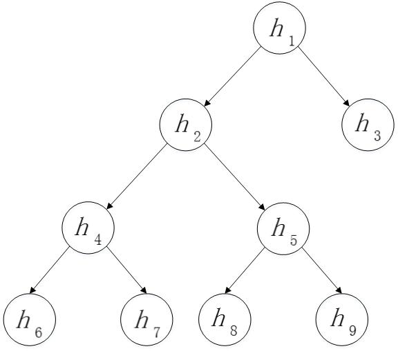
Figure 4: Top-down tree LSTM.

Note, however, that two different sets of model parameters are used when the current node is the left and the right child of its predecessor, respectively. Denoting the two sets of parameters as $\mathbf{U}_{L}$ and $\mathbf{U}_{R}$, respectively, the hidden state vector $h_{7}$ in Figure 4 is calculated from the hidden state vector $h_{1}$ using the parameter set sequence $[\mathbf{U}_{L},\mathbf{U}_{L},\mathbf{U}_{R}]$. Similarly, $h_{8}$ is calculated from $h_{1}$ using $[\mathbf{U}_{L},\mathbf{U}_{R},\mathbf{U}_{L}]$. At each step $t$, the computing of $h_{t}$ follows the sequential LSTM model:

$$\begin{split}h_{t}&=o_{t}\otimes\tanh(c_{t-1})\\ c_{t}&=f_{t}\otimes c_{t-1}+i_{t}\otimes g_{t}\\ g_{t}&=\tanh(W_{xg\downarrow}^{N}x_{t-1}+W_{hg\downarrow}^{N}h_{t-1}+b_{g\downarrow}^{N})\\ \end{split}$$ (14)

With the gate values being defined as:

$$\begin{split}i_{t}&=\sigma(W_{xi\downarrow}^{N}x_{t}+W_{hi\downarrow}^{N}h_{t-1}+W_{ci\downarrow}^{N}c_{t-1}+b_{i\downarrow}^{N})\\ f_{t}&=\sigma(W_{xf\downarrow}^{N}x_{t}+W_{hf\downarrow}^{N}h_{t-1}+W_{cf\downarrow}^{N}c_{t-1}+b_{f\downarrow}^{N})\\ o_{t}&=\sigma(W_{xo\downarrow}^{N}x_{t}+W_{ho\downarrow}^{N}h_{t-1}+W_{co\downarrow}^{N}c_{t}+b_{o\downarrow}^{N})\\ \end{split}$$ (15)

Here $N\in\{L,R\}$ and $\mathbf{U}_{N}=\{W_{xg\downarrow}^{N},W_{hg\downarrow}^{N},\\ b_{g\downarrow}^{N},W_{xi\downarrow}^{N},W_{hi\downarrow}^{N},W_{ci\downarrow}^{N},b_{i\downarrow}^{N},W_{xf\downarrow}^{N},W_{hf\downarrow}^{N},W_{cf\downarrow}^{N},b_{f\downarrow}^{N},\\ W_{xo\downarrow}^{N},W_{ho\downarrow}^{N},W_{co\downarrow}^{N},b_{o\downarrow}^{N}\}$. $\mathbf{U}_{L}$ and $\mathbf{U}_{R}$ are model parameters in the top-down Tree LSTM.

One final note is that the top-down Tree LSTM is enabled by the head propagation mechanism, which allows a head lexicon node to be made available for the root constituent node. Without such information, it would be difficult to build top-down LSTM for constituent trees.

5 Classification

We apply the bidirectional Tree LSTM to classification tasks, where the input is a sentence with its binarized constituent tree, and the output is a discrete label. Denoting the bottom-up hidden state vector of the root as $\tilde{h}_{ROOT\uparrow}$, the top-down hidden state vector of the root as $\tilde{h}_{ROOT\downarrow}$ and the top-down hidden state vectors of the input words $x_{1}$, $x_{2}$, …, $x_{n}$ as $\tilde{h}_{1}^{\prime}$, $\tilde{h}_{2}^{\prime}$, …, $\tilde{h}_{n}^{\prime}$, respectively, we take the concatenation of $\tilde{h}_{ROOT\uparrow}$, $\tilde{h}_{ROOT\downarrow}$ and the average of $\tilde{h}_{1}^{\prime}$, $\tilde{h}_{2}^{\prime}$, …, $\tilde{h}_{n}^{\prime}$ as the final representation $h$ of the sentence:

$$h=\tilde{h}_{ROOT\uparrow}\oplus\tilde{h}_{ROOT\downarrow}\oplus\frac{1}{n}\sum_{i=1}^{n}\tilde{h}_{i}^{\prime}$$ (16)

A softmax classifier is used to predict the probability $p_{j}$ of sentiment label $j$ from $h$ by

$$\begin{split}h_{l}&=\text{ReLU}(W_{hl}h+b_{hl})\\ P&=\text{\emph{softmax}}(W_{lp}h_{l}+b_{lp})\\ p_{j}&=P[j],\\ \end{split}$$ (17)

where $W_{hl}$, $b_{hl}$, $W_{lp}$ and $b_{lp}$ are model parameters, and ReLU is the rectifier function $f(x)=\max(0,x)$. During prediction, the largest probability component of $P$ will be taken as the answer.

6 Training

We train our classifier to maximize the conditional log-likelihood of gold labels of training samples. Formally, given a training set of size $|D|$, the training objective is defined by

$$L(\theta)=-\sum_{i=1}^{|D|}\log p_{y_{i}}+\frac{\lambda}{2}||\theta||^{2},$$ (18)

where $\theta$ is the set of model parameters, $\lambda$ is a regularization parameter, $y_{i}$ is the gold label of the $i$-th training sample and $p_{y_{i}}$ is obtained according to Equation 17. For sequential LSTM models, we collect errors over each sequence. For Tree LSTMs, we sum up errors at every node.

The model parameters are optimized using ADAM [Kingma and Ba, 2014] without gradient clipping, with the default hyper-parameters of the AdamTrainer in the Dynet toolkits. We also use dropout [Srivastava et al., 2014] at lexical input embeddings with a fixed probability $p_{drop}$ to avoid overfitting. $p_{drop}$ is set to 0.5 for all tasks.

Following ?), ?), ?) and ?), we use Glove-300d word embeddings to train our model. The pretrained word embeddings are fine-tuned for all tasks. Unknown words are handled in two steps. First, if a word is not contained in the pretrained word embeddings, but its lowercased form exists in the embedding table, we use the lowercase as a replacement. Second, if both the original word and its lowercased form cannot be found, we treat the word as unk. The embedding vector of the UNK token is initialized as the average of all embedding vectors.

We use one hidden layer and same dimensionality settings for both sequential and Tree LSTMs. LSTM hidden states are of size 150. The output hidden size is 128 and 64 for the sentiment classification task and the question type classification task, respectively. Each model is trained for 30 iterations. The same training procedure is repeated for 5 times using different random seeds, with parameters being evaluated at the end of every iteration on the development set. We use the label accuracy to select the best model over the 5 development runs and across the 30 iterations, which is taken for the final test.

7 Experiments

7.1 Data

The effectiveness of our model is tested on a sentiment classification task and a question type classification task.

7.1.1 Sentiment Classification

For sentiment classification, we use the same data settings as ?). Specifically, the Stanford Sentiment Treebank [Socher et al., 2013b] is used to train our classification model, which contains sentiments for movie reviews. Each sentence is annotated with a constituent tree.Every internal node corresponds to a phrase. Each node is manually assigned an integer sentiment label from 0 to 4, which respectively correspond to five sentiment classes: very negative, negative, neutral, positive and very positive. The root label represents the sentiment label of the whole sentence.

We perform both binary classification and fine-grained classification. Following previous work, we use labels of all phrases for training. Gold-standard tree structures are used for training and testing [Le and Zuidema, 2015, Li et al., 2015, Zhu et al., 2015b, Tai et al., 2015]. Accuracies are evaluated for both the sentence root labels and phrase labels.

7.1.2 Question Type Classification

For the question type classification task, we use the TREC data [Li and Roth, 2002]. Each training sample in this dataset contains a question sentence and its corresponding question type. We work on the six-way coarse classification task, where the six question types are ENTY, HUM, LOC, DESC, NUM and ABBR, corresponding to ENTITY, HUMAN, LOCATION, DESCRIPTION, NUMERIC VALUE and ABBREVIATION, respectively. For example, the correct type for the sentence “What year did the Titanic sink?” is of the NUM type. The training set consists of 5,452 examples and the test set contains 500 examples. Since there is no development set, we follow ?), randomly extracting 500 examples from the training set as a development set. Different from the sentiment treebank, there is no annotated tree for each sentence. Instead, we obtain an automatically parsed tree for each sentence using an open-sourced parser off-the-shelf (ZPar). Another difference between the TREC data and the sentiment treebank is that there is only one label, at the root node, rather than a label for each phrase.

7.2 Baselines

We consider two models for our baselines. The first is a bidirectional LSTM (BiLSTM) [Hochreiter and Schmidhuber, 1997, Graves et al., 2013]. Our bidirectional constituency Tree LSTM (BiConTree) are compared with the bidirectional sequential LSTM to investigate the effectiveness of the tree structure. For the sentiment task, following ?) and ?), we convert the treebank into sequences to allow the bidirectional LSTM model to make use of every phrase span as a training example. The second baseline model is the bottom-up Tree LSTM model of ?). We make a contrast between this model and our lexicalized bidirectional models to show the effects of adding head lexicalization and top-down information flow.

7.3 Main Results

Table 1 shows the main results for the sentiment classification task, where RNTN is the recursive neural tensor model of ?), ConTree and DepTree denote constituency Tree LSTMs and dependency Tree LSTMs, respectively. Our re-implementation of sequential bidirectional LSTM and constituent Tree LSTM [Zhu et al., 2015b] gives comparable results to ?)’s original implementation.

Model	5-class		binary
	Root	Phrase	Root	Phrase
RNTN[Socher et al., 2013b]	45.7	80.7	85.4	87.6
BiLSTM[Li et al., 2015]	49.8	83.3	86.7	-
DepTree[Tai et al., 2015]	48.4	-	85.7	-
ConTree[Le and Zuidema, 2015]	49.9	-	88.0	-
ConTree[Zhu et al., 2015b]	50.1	-	-	-
ConTree[Li et al., 2015]	50.4	83.4	86.7	-
ConTree[Tai et al., 2015]	51.0	-	88.0	-
BiLSTM (Our implementation)	49.9	82.7	87.6	91.8
ConTree (Our implementation)	51.2	83.0	88.5	92.5
Top-down ConTree	51.0	82.9	87.8	92.1
ConTree + Lex	52.8	83.2	89.2	92.3
BiConTree	53.5	83.5	90.3	92.8

Table 1: Test set accuracies for sentiment classification tasks.

After incorporating head lexicalization into our constituent Tree LSTM, the fine-grained sentiment classification accuracy increases from $51.2$ to $52.8$, and the binary sentiment classification accuracy increases from $88.5$ to $89.2$, which demonstrates the effectiveness of the head lexicalization mechanism.

Table 1 also shows that a vanilla top-down ConTree LSTM enabled by head-lexicalization (i.e. the top-down half of the final bidirectional model) alone obtains comparable accuracies to the bottom-up ConTree LSTM model. The BiConTree model can further improve the classification accuracies by 0.7 points (fine-grained) and 1.3 points (binary) compared to the unidirectional bottom-up lexicalized ConTree LSTM model, respectively.

Table 1 includes 5 class accuracies for all nodes. There is no significant difference between different models, as consistent with the observation of ?). To our knowledge, these are the best reported results for this sentiment classification task until now.

Table 2 shows the question type classification results. Our final model gives better results compared to the BiLSTM model and the bottom-up ConTree model, achieving comparable results to the state-of-the-art, which is a SVM classifier with carefully designed features.

Model	Accuracy
Baseline BiLSTM	93.8
Baseline BottomUp ConTree LSTM	93.4
SVM [Silva et al., 2011]	95.0
Bidirectional ConTree LSTM	94.8

Table 2: TREC question type classification results.

Method	L	R	A	G
Root Accuracy (%)	51.1	51.6	51.8	53.5

Table 3: Test set accuracies of four head lexicalization methods on fine-grained classification.

7.4 Training Time and Model Size

Introducing head lexicalization and bidirectional extension to the model increases the model complexity. In this section, we analyze our model in terms of training time and model size on the fine-grained sentiment classification task.

Model	ConTree	ConTree+Lex	BiConTree
Time (s)	4,664	7,157	11,434

Table 4: Averaged training time over 30 iterations.

We run all the models using an i7-4790 3.60GHz CPU with a single thread. Table 4 shows the average running time for different models over 30 iterations. The baseline ConTree model takes about 1.3 hours to finish the training procedure. ConTree+Lex takes about 1.5 times longer than ConTree. BiConTree takes about 3.2 hours, which is about 2.5 times longer than that of ConTree.

Model	$|h|$	#Parameter	Accuracy (%)
ConTree	150	538,223	51.2
ConTree+Lex	75	376,673	51.5
ConTree+Lex	150	763,523	52.8
ConTree+Lex	215	1,253,493	52.5
ConTree+Lex	300	2,110,973	51.8
BiConTree	75	564,923	52.6
BiConTree	150	1,297,523	53.5

Table 5: Effect of model size.

Table 5 compares the model sizes. We did not count the number of parameters in the lookup table since these parameters are the same for all models. Since the size of LSTM models mainly depends on the dimensionality of the state vector $h$, we change the size of $h$ for comparing the effect of model size. When $|h|=150$, the model size of the baseline model ConTree is the smallest, which consists of about 538K parameters. The model size of ConTree+Lex is about 1.4 times as large as that of the baseline model. The bidirectional model BiConTree is the largest, which is about 1.7 times as large as that of the ConTree+Lex model. However, this parameter set is not very large compared to the modern memory capacity, even for a computer with 16GB RAM. In conclusion, in terms of both time, model size and accuracy, head lexicalization method is a good choice.

Table 5 also helps to clarify whether the gain of the BiConTree model over the ConTree+Lex model is from the top-down information flow or more parameters. For the same model, increasing the model size can improve the performance to some extent. For example, doubling the size of $|h|$ ($75\rightarrow 150$) increases the performance from $51.5$ to $52.8$ for the ConTree+Lex model. Similarly, we boost the performance of the BiConTree model when doubling the size of $|h|$ from $75$ to $150$. However, continuing doubling the size of $|h|$ from $150$ to $300$ empirically decreases the performance of the ConTree+Lex model. The BiConTree model with $|h|=75$ is much smaller than the ConTree+Lex model with $|h|=150$ in terms of model size. However the performance of these two models is quite close, which indicates that top-down information is useful even for a small model. We also run a ConTree+Lex model with $|h|=215$, the model size of which is similar to that of the BiConTree model with $|h|=150$. The performance of the ConTree+Lex model is still worse than the BiConTree model ($52.5$ v.s. $53.5$), which shows the effectiveness of top-down information.

7.5 Head Lexicalization Methods

In this experiment, we investigate the effect of our head lexicalization method over heuristic baselines. We consider three baseline methods, namely L, R and A. For L, a parent node accepts lexical information of its left child while ignoring the right child. Correspondingly, for R, a parent node accepts lexical information of its right child while ignoring the left child. For A, a parent node averages the lexical vectors of the left and right child.

Table 3 shows the accuracies on the test set, where G denotes our method described in Section 4.1. R gives better results compared to L due to relatively more right-branching structures in this treebank.A simple average yields similar results compared with right branching. In contrast, G outperforms A method by considering the relative weights of each branch according to tree-level contexts.

(a) “Emerges as something rare”.

(b) “is a good place to start”.

(c) “the road to hell is paved with good intentions”.

Figure 5: Visualizing head words found automatically by our model.

We then investigate what lexical heads can be learned by G. Interestingly, the lexical heads contain both syntactic and sentiment information: while some heads correspond well to Collins syntactic rules [Collins, 2003], others are driven by subjective words. Compared to Collins’ rules, our method found 30.68% and 25.72% overlapping heads on the dev set and test set, respectively.

Figure 5 shows some visualization based on the cosine similarity between the head lexical vector and its children. We decide the head of a node by choosing the head of the child that gives the largest similarity value. Some examples are shown below, where $<>$ is used to indicate head words. Sentiment labels (e.g. 2, 3) are also included. In Figure 5(a), “Emerges” is the syntactic head word of the whole phrase, which is consistent with Collins-style head finding. However, “rare” is the head word of the phrase “something rare”, which is different from the syntactic head, but rather sentiment-related. Similar observations are found in Figure 5(b), where “good” is the head word of the whole phrase, rather than the syntactic head “place”. The sentiment label of “good” and the sentiment label of the whole phrase are both 3. Figure 5(c) shows more complex interactions between syntax and sentiment for deciding the head word.

7.6 Error Analysis

Table 6 shows some example sentences incorrectly predicted by the baseline bottom-up tree model, but correctly labeled by our final model.

ID	sentence	baseline	our model
1	Gloriously goofy ( and gory ) midnight movie stuff .	negative	positive
2	The film is really not so much bad as bland .	positive	negative
3	This is a good movie in spurts , but when it does n’t work , it ’s at important times .	positive	neutral

Table 6: Example output sentences.

The head word of sentence #1 by our model is “Gloriously”, which is consistent with the sentiment of the whole sentence. This shows how head lexicalization can affect sentiment classification results. Sentences #2 and #3 show the usefulness of top-down information for complex semantic structures, where compositionality exhibits subtle effects. With top-down LSTM, the models can predict the sentiment labels correctly. Our final model improves the results for the ‘very negative’ and ‘very positive’ classes by 10% and 11%, respectively. It also boosts the accuracies for sentences with negation (e.g. “not”, “no”, and “none”) by 4.4%.

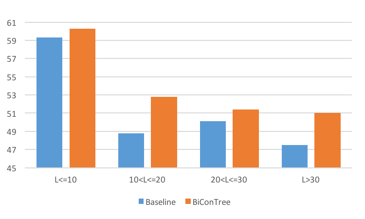
Figure 6: Distribution of 5-class accuracies at the root level according to the sentence length.

Figure 6 shows the accuracy distribution according to the sentence length. We find that our model can improve the classification accuracy for longer sentences ($>$30 words) by 3.5 points compared to the baseline ConTree LSTM of ?), which demonstrates the strength of our model for handling long range information. By considering bidirectional information over tree structures, our model is aware of more complicate contexts for making better predictions.

7.7 Parser Reranking

Model	$F_{1}$
Baseline (?))	90.40
ConTree	90.70
ConTree+Lex	90.83
Our 8-best Oracle	92.59

Table 7: Neural reranking results on WSJ test set.

Our main results are obtained on semantic-driven tasks, where the automatically-learned head words contain mixed syntactic and semantic information. To further investigate the effectiveness of automatically learned head information on a pure syntactic task, we additionally conduct a simple parser reranking experiment. The standard PTB [Marcus et al., 1993] split [Collins, 2003] are used, and the same off-the-shelf ZPar model is adopted for our baseline. A standard interpolated reranker [Zhu et al., 2015a, Zhou et al., 2016] is adopted for scoring 8-best trees. For each tree y of sentence x, we follow ?) to define $f(x,y;\Theta)$ as the sum of scores of each constituent node,

$$f(x,y;\Theta)=\sum\limits_{r\in\text{node}{(x,y)}}{Score(r;\Theta)}$$ (19)

Without loss of generality, we take a binary node as an example. Given a node A, suppose that its two children are B and C. Let the learned composition state vectors of A, B and C by our proposed Tree-LSTM model be $N_{A}$, $N_{B}$ and $N_{C}$, respectively. The head word vector of node A is ${H}_{A}$. $Score(A;\Theta)$ is defined as:

$$\small\begin{split}&O_{(A\rightarrow BC)}=ReLU(W_{s}^{L}N_{B}+W_{s}^{R}N_{C}+W_{s}^{H}H_{A}+b^{s})\\ &\text{Score}_{(A\rightarrow BC)}=\log(softmax(O_{(A\rightarrow B\ C)}))[A],\end{split}$$ (20)

where $W_{s}^{L}$, $W_{s}^{R}$ and $b^{s}$ are model parameters, which are trained using a margin loss.

Table 7 shows the reranking results on WSJ test set. The baseline F1 score is 90.40. Our ConTree improves the baseline model from $90.40$ to $90.70$. Using ConTree+Lex model can further improve the performance ($90.70\rightarrow 90.83$). This serves as an evidence that automatic heads can also be useful to some extent for a syntactic task, despite that our main motivation is more semantic-driven. Among neural rerankers, out model outperforms ?), but is not as good as current state-of-the-art models, including sequence-to-sequence based LSTM language models [Vinyals et al., 2015, Charniak, 2016] and recurrent neural network grammars [Dyer et al., 2016], due to a low baseline oracle and simple reranking models. Nevertheless, it serves our goal of contrasting the tree LSTM models.

8 Conclusion

We showed that existing LSTM models for constituent tree structures are limited by not considering direct lexical input in the computing of cell values for non-leaf constituents, and proposed a head-lexicalization method to address this issue. Learning the heads of constituent automatically using a neural model, our lexicalized tree LSTM is applicable to arbitrary binary branching trees in form of CFG, and is formalism-independent. In addition, lexical information on the root further allows a top-down extension to the model, resulting in a bi-directional constituent Tree LSTM. Experiments on two well-known datasets show that head-lexicalization improves the unidirectional Tree LSTM model, and bidirectional Tree LSTM gives superior labeling results compared with both unidirectional Tree LSTMs and bidirectional sequential LSTMs. We release our code under GPL at XXX.

References

- [Bahdanau et al., 2014] Dzmitry Bahdanau, Kyunghyun Cho, and Yoshua Bengio. 2014. Neural machine translation by jointly learning to align and translate. arXiv preprint arXiv:1409.0473.
- [Charniak, 2016] Eugene Charniak. 2016. Parsing as language modeling.
- [Clark and Curran, 2004] Stephen Clark and James R. Curran. 2004. Parsing the wsj using ccg and log-linear models. In Proceedings of the 42nd Meeting of the Association for Computational Linguistics (ACL’04), Main Volume, pages 103–110, Barcelona, Spain, July.
- [Collins, 2003] Michael Collins. 2003. Head-driven statistical models for natural language parsing. Computational linguistics, 29(4):589–637.
- [Collobert and Weston, 2008] Ronan Collobert and Jason Weston. 2008. A unified architecture for natural language processing: Deep neural networks with multitask learning. In Proceedings of the 25th international conference on Machine learning, pages 160–167. ACM.
- [Dyer et al., 2015] Chris Dyer, Miguel Ballesteros, Wang Ling, Austin Matthews, and Noah A. Smith. 2015. Transition-based dependency parsing with stack long short-term memory. In ACL.
- [Dyer et al., 2016] Chris Dyer, Adhiguna Kuncoro, Miguel Ballesteros, and Noah A Smith. 2016. Recurrent neural network grammars. arXiv preprint arXiv:1602.07776.
- [Elman, 1990] Jeffrey L Elman. 1990. Finding structure in time. Cognitive science, 14(2):179–211.
- [Gers and Schmidhuber, 2000] Felix A Gers and Jürgen Schmidhuber. 2000. Recurrent nets that time and count. In Neural Networks, 2000. IJCNN 2000, Proceedings of the IEEE-INNS-ENNS International Joint Conference on, volume 3, pages 189–194. IEEE.
- [Graves et al., 2013] Alan Graves, Navdeep Jaitly, and Abdel-rahman Mohamed. 2013. Hybrid speech recognition with deep bidirectional lstm. In Automatic Speech Recognition and Understanding (ASRU), 2013 IEEE Workshop on, pages 273–278. IEEE.
- [Hochreiter and Schmidhuber, 1997] Sepp Hochreiter and Jürgen Schmidhuber. 1997. Long short-term memory. Neural computation, 9(8):1735–1780.
- [Kingma and Ba, 2014] Diederik P. Kingma and Jimmy Ba. 2014. Adam: A method for stochastic optimization. CoRR, abs/1412.6980.
- [Klein and Manning, 2003] Dan Klein and Christopher D Manning. 2003. Accurate unlexicalized parsing. In Proceedings of the 41st Annual Meeting on Association for Computational Linguistics-Volume 1, pages 423–430. Association for Computational Linguistics.
- [Le and Zuidema, 2015] Phong Le and Willem Zuidema. 2015. Compositional distributional semantics with long short term memory. In Proceedings of the Fourth Joint Conference on Lexical and Computational Semantics, pages 10–19, Denver, Colorado, June. Association for Computational Linguistics.
- [Li and Roth, 2002] Xin Li and Dan Roth. 2002. Learning question classifiers. In Proceedings of the 19th international conference on Computational linguistics-Volume 1, pages 1–7. Association for Computational Linguistics.
- [Li et al., 2015] Jiwei Li, Minh-Thang Luong, Dan Jurafsky, and Eudard Hovy. 2015. When are tree structures necessary for deep learning of representations? In Empirical Methods in Natural Language Processing (EMNLP).
- [Marcus et al., 1993] Mitchell P Marcus, Mary Ann Marcinkiewicz, and Beatrice Santorini. 1993. Building a large annotated corpus of english: The penn treebank. Computational linguistics, 19(2):313–330.
- [Mikolov et al., 2010] Tomas Mikolov, Martin Karafiát, Lukas Burget, Jan Cernockỳ, and Sanjeev Khudanpur. 2010. Recurrent neural network based language model. INTERSPEECH, 2:3.
- [Mikolov et al., 2013] Tomas Mikolov, Kai Chen, Greg Corrado, and Jeffrey Dean. 2013. Efficient estimation of word representations in vector space. arXiv preprint arXiv:1301.3781.
- [Miwa and Bansal, 2016] Makoto Miwa and Mohit Bansal. 2016. End-to-end Relation Extraction using LSTMs on Sequences and Tree Structures. ArXiv e-prints, abs/1601.00770, January.
- [Paulus et al., 2014] Romain Paulus, Richard Socher, and Christopher D Manning. 2014. Global belief recursive neural networks. In Advances in Neural Information Processing Systems, pages 2888–2896.
- [Silva et al., 2011] Joao Silva, Luísa Coheur, Ana Cristina Mendes, and Andreas Wichert. 2011. From symbolic to sub-symbolic information in question classification. Artificial Intelligence Review, 35(2):137–154.
- [Socher et al., 2011] Richard Socher, Cliff C. Lin, Andrew Y. Ng, and Christopher D. Manning. 2011. Parsing Natural Scenes and Natural Language with Recursive Neural Networks. In Proceedings of the 26th International Conference on Machine Learning (ICML).
- [Socher et al., 2013a] Richard Socher, John Bauer, Christopher D. Manning, and Ng Andrew Y. 2013a. Parsing with compositional vector grammars. In Proceedings of the 51st Annual Meeting of the Association for Computational Linguistics (Volume 1: Long Papers), pages 455–465, Sofia, Bulgaria, August. Association for Computational Linguistics.
- [Socher et al., 2013b] Richard Socher, Alex Perelygin, Jean Wu, Jason Chuang, Christopher Manning, Andrew Ng, and Christopher Potts. 2013b. Recursive deep models for semantic compositionality over a sentiment treebank. In EMNLP.
- [Srivastava et al., 2014] Nitish Srivastava, Geoffrey Hinton, Alex Krizhevsky, Ilya Sutskever, and Ruslan Salakhutdinov. 2014. Dropout: A simple way to prevent neural networks from overfitting. The Journal of Machine Learning Research, 15(1):1929–1958.
- [Sutskever et al., 2014] Ilya Sutskever, Oriol Vinyals, and Quoc V Le. 2014. Sequence to sequence learning with neural networks. In Advances in neural information processing systems, pages 3104–3112.
- [Tai et al., 2015] Kai Sheng Tai, Richard Socher, and Christopher D. Manning. 2015. Improved semantic representations from tree-structured long short-term memory networks. In Association for Computational Linguistics (ACL).
- [Vinyals et al., 2015] Oriol Vinyals, Łukasz Kaiser, Terry Koo, Slav Petrov, Ilya Sutskever, and Geoffrey Hinton. 2015. Grammar as a foreign language. In Advances in Neural Information Processing Systems, pages 2755–2763.
- [Zhang et al., 2015] Xingxing Zhang, Liang Lu, and Mirella Lapata. 2015. Tree recurrent neural networks with application to language modeling. CoRR, abs/1511.00060.
- [Zhou et al., 2015] Chunting Zhou, Chonglin Sun, Zhiyuan Liu, and Francis C. M. Lau. 2015. A C-LSTM neural network for text classification. CoRR, abs/1511.08630.
- [Zhou et al., 2016] Hao Zhou, Yue Zhang, Shujian Huang, Junsheng Zhou, Xin-Yu Dai, and Jiajun Chen. 2016. A search-based dynamic reranking model for dependency parsing. In Proceedings of the 54th Annual Meeting of the Association for Computational Linguistics (Volume 1: Long Papers), pages 1393–1402, Berlin, Germany, August. Association for Computational Linguistics.
- [Zhu et al., 2013] Muhua Zhu, Yue Zhang, Wenliang Chen, Min Zhang, and Jingbo Zhu. 2013. Fast and accurate shift-reduce constituent parsing.
- [Zhu et al., 2015a] Chenxi Zhu, Xipeng Qiu, Xinchi Chen, and Xuanjing Huang. 2015a. A re-ranking model for dependency parser with recursive convolutional neural network. In Proceedings of the 53rd Annual Meeting of the Association for Computational Linguistics and the 7th International Joint Conference on Natural Language Processing (Volume 1: Long Papers), pages 1159–1168, Beijing, China, July. Association for Computational Linguistics.
- [Zhu et al., 2015b] Xiaodan Zhu, Parinaz Sobhani, and Hongyu Guo. 2015b. Long short-term memory over tree structures. CoRR, abs/1503.04881.