Aging and linear response in the Hébraud-Lequeux model for amorphous rheology

Abstract

We analyse the aging dynamics of the Hébraud-Lequeux model, a self-consistent stochastic model for the evolution of local stress in an amorphous material. We show that the model exhibits initial-condition dependent freezing: the stress diffusion constant decays with time as $D\sim 1/t^{2}$ during aging so that the cumulative amount of memory that can be erased, which is given by the time integral of $D(t)$, is finite. Accordingly the shear stress relaxation function, which we determine in the long-time regime, only decays to a plateau and becomes progressively elastic as the system ages. The frequency-dependent shear modulus exhibits a corresponding overall decay of the dissipative part with system age, while the characteristic relaxation times scale linearly with age as expected.

1 Introduction

The prediction and modelling of the mechanical behaviour and flow of amorphous materials is an active area of research, reviewed recently in e.g. [1, 2, 3]. Because identifying flow events – as the analogue of dislocation motion in crystalline solids – remains a challenge for microscopic models, mesoscopic models have been proposed as one strand of this research effort, with the goal of capturing some of the salient physics without resorting to a detailed particle-based description. Among such mesoscopic models are Shear Transformation Zone theory [4, 5, 6], the soft glassy rheology (SGR) model [7, 8, 9, 10], fluidity models (see e.g. [11]) and the Hébraud-Lequeux (HL) model [12] and its variants. The latter is a stochastic model describing the evolution of the shear stress $\sigma$ of a local element of material, under the influence of an externally applied shear strain $\gamma$ and stochastic noise arising from flow events elsewhere in the material that perturb the local stress.

The HL model, like the STZ and SGR models in their original formulations, is a “one-element” model that contains coupling to other elements of the material only via a self-consistency requirement for the noise level. But it has also been obtained in approximate treatments of more complicated models that explicitly represent the spatial structure of the amorphous material under study [13, 14, 15]. This makes it important to understand fully the predictions of the HL model. These have been worked out for steady shear (constant $\dot{\gamma}$), leading to the flow curve $\sigma_{\rm ss}(\dot{\gamma})$ giving steady state shear stress versus shear rate [12]. The main control parameter $\alpha$ regulates how strongly flow events elsewhere affect a given local element of material. For high $\alpha$ ($\alpha>1/2$), the flow curve is linear at small shear rates, $\sigma_{\rm ss}\propto\dot{\gamma}$, representing Newtonian flow. For small $\alpha$, on the other hand, a nonzero yield stress $\sigma_{\rm ss}(\dot{\gamma}\to 0)$ appears: for (average) stress below this value a steady flow cannot then be maintained. This regime can therefore be identified as the “glassy” one, where the amorphous material has acquired solid-like properties, and $\alpha=1/2$ gives the location of the corresponding glass transition [12, 16].

The glassy regime of the HL model was analysed in the original paper [12] only in steady states driven either by steady flow, as above, or by oscillatory strain $\gamma(t)=\gamma_{0}\cos(\omega t)$ of some nonzero amplitude $\gamma_{0}$. In the absence of strain, however, one expects the model to display aging, i.e. its properties should depend on the “waiting time” $t_{\rm w}$ since the system was prepared, also called the age of the system. The linear stress response to an applied step strain, also called the stress relaxation function, then becomes a function $G(t,t_{\rm w})$ of both the age $t_{\rm w}$ when the perturbation is applied, and the time $t$ when the stress response is measured. The goal of this paper is to establish the aging behaviour of the HL model, with a particular focus on $G(t,t_{\rm w})$ and its frequency-domain analogue.

In Sec. 2 we introduce the HL model and our approach for calculating its linear response to applied strain in the aging regime. We focus on the long-time regime throughout in our analysis, which for two-time quantities like the stress relaxation function $G(t,t_{\rm w})$ means that we will consider both times large but with fixed ratio $t/t_{\rm w}=1+x$, i.e. we take $t_{\rm w}\to\infty$ at fixed $x$.

In Sec. 3 we describe the aging behaviour of the HL model in the absence of applied strain, leaving most details of the analysis to an appendix. One of the main results will be that stochastic effects die out so quickly in the glassy regime that even after an infinite time they are not sufficient to erase memory of the initial preparation of the system.

The discussion of the linear stress response is split into two parts: in Sec. 4 we give qualitative arguments for the behaviour of $G(t,t_{\rm w})$ in the long-time regime. A precise quantitative analysis requires the use of boundary layer scaling techniques, which we discuss in Sec. 5. The use of these techniques, which were developed previously for the HL model in [17, 16], is the main technical contribution of this paper, making it rather distinct from approaches – e.g. temporal Laplace transforms – used to analyse aging in other mesoscopic models for amorphous rheology such as SGR [8].

We translate our results into the frequency domain in Sec. 6, which corresponds to the experimentally common technique of probing linear stress response to oscillatory strain. In Sec. 7, finally, we compare results from a numerical solution of the HL model to the predicted long-time asymptotics, finding good agreement. A short summary and discussion of our results is provided in Sec. 8.

2 The HL model

In dimensionless units, the Hébraud-Lequeux model describes the time evolution of a stress distribution $p(\sigma,t)$ as

$$\partial_{t}p(\sigma,t)=-\dot{\gamma}\partial_{\sigma}p+D\partial_{\sigma}^{2}p-h(\sigma)p+\Gamma\delta(\sigma)$$ (1)

where $h(\sigma)=\Theta(|\sigma|-1)$ and the yield rate $\Gamma(t)$ is determined by

$$\Gamma(t)=\int d\sigma\,h(\sigma)p(\sigma,t)\ .$$ (2)

as required for conservation of probability, $\int d\sigma\,p(\sigma,t)=1$.

The interested reader is referred to [12] for more details on the model and its interpretation. Briefly, $p(\sigma,t)$ can be viewed as the distribution of shear stresses across all local elements of an amorphous material. The first term on the r.h.s. of (1) represents elastic response $\dot{\sigma}=\dot{\gamma}$ of the stress $\sigma$ to the applied strain $\gamma$; the relevant elastic shear modulus has been scaled to unity. The third term describes yielding: once the local stress $\sigma$ exceeds a yield stress, which is again scaled to unity, a yield event occurs with unit rate. Physically this corresponds to a rearrangement of particles that relaxes the stress in an element to zero, as represented by the fourth term on the r.h.s. of (1). The yield rate, i.e. the overall at which such events take place, is $\Gamma$.

The key self-consistent aspect of the model lies in the second term in (1): yield events occurring elsewhere in the material will perturb the local stress of an element. The assumption of the model is that this perturbation can be described as Gaussian noise with a stress diffusion constant that is proportional to the yield rate, $D(t)=\alpha\Gamma(t)$. (We use the conventional name “diffusion constant” but note that $D(t)$ in general depends on time.) Here $\alpha$ encodes the interaction strength between elements, or alternatively the ability of the system to propagate mechanical noise, and is the key control parameter of the model. The overall macroscopic stress is assumed to be given by the average $\langle\sigma\rangle=\int d\sigma\,\sigma p(\sigma,t)$.

For the analysis of aging in the HL model in the absence of applied strain, we will study the solution of (1) for $\dot{\gamma}=0$; see Sec. 3. We then move to the linear response of the stress to small applied strains $\gamma(t)$, for an aging system at $\alpha<1/2$. The simplest perturbation scenario, from which all other linear response functions can be calculated, is a step in $\gamma(t)$ at time $t_{\rm w}$, $\gamma(t)=\gamma_{0}\Theta(t-t_{\rm w})$ with small amplitude $\gamma_{0}$. Then for $t>t_{\rm w}$ we can expand $p$ as follows

$$p(\sigma,t)=p_{0}(\sigma,t)+\gamma_{0}\delta p(\sigma,t)+O(\gamma_{0}^{2}).$$ (3)

For the stress diffusion constant we have in principle similarly $D(t)=D_{0}(t)+\gamma_{0}\delta D(t)+O(\gamma_{0}^{2})$ but it turns out that the first order perturbation $\delta D(t)$ vanishes provided we make an assumption that we will use throughout the paper, namely that the initial system preparation produces a symmetric stress distribution, $p_{0}(\sigma,0)=p_{0}(-\sigma,0)$.

To see why $\delta D(t)=0$, note generally that (1) is invariant under the joint transformation $p(\sigma,t)\to p(-\sigma,t)$ and $\gamma(t)\to-\gamma(t)$. In the absence of strain, symmetry of the stress distribution is therefore preserved by the time evolution, i.e. if as assumed $p_{0}(\sigma,0)$ is symmetric then so is $p_{0}(\sigma,t)$ for all $t$. With the step strain added, the invariance of the time evolution under joint sign reversal of $\sigma$ and $\gamma_{0}$ then implies that

$$p_{0}(\sigma,t)+\gamma_{0}\delta p(\sigma,t)+O(\gamma_{0}^{2})$$ (4)

and

$$p_{0}(-\sigma,t)-\gamma_{0}\delta p(-\sigma,t)+O(\gamma_{0}^{2})$$ (5)

are both solutions of the master equation. Because of the assumed symmetry of $p_{0}$ and uniqueness of the solution for given $p_{0}(\sigma,0)$ and $\gamma_{0}$ this tells us that $\delta p(\sigma,t)=-\delta p(-\sigma,t)$: $\delta p$ is an odd function of $\sigma$, and hence $\delta D(t)=\alpha\int d\sigma\,h(\sigma)\delta p(\sigma,t)$ vanishes.

Expanding the master equation (1) in $\gamma_{0}$ and using $\delta D(t)=0$ gives then, by comparing the $O(1)$ and $O(\gamma_{0})$ contributions on both sides,

$$\partial_{t}p_{0}(\sigma,t)=D_{0}(t)\partial_{\sigma}^{2}p_{0}(\sigma,t)-h(\sigma)p_{0}(\sigma,t)+\frac{D_{0}(t)}{\alpha}\delta(\sigma)$$ (6)

as expected, and

$$\partial_{t}\delta p(\sigma,t)=D_{0}(t)\partial_{\sigma}^{2}\delta p(\sigma,t)-h(\sigma)\delta p(\sigma,t)$$ (7)

The initial condition for $\delta p$ can be obtained by integrating (1) across a small time interval around $t_{\rm w}$, bearing in mind that $\dot{\gamma}(t)=\gamma_{0}\delta(t-t_{\rm w})$. This yields

$$\delta p(\sigma,t_{\rm w})=-\partial_{\sigma}p_{0}(\sigma,t_{\rm w})$$ (8)

where the l.h.s. is to be understood as the limit of $\delta p(\sigma,t)$ for $t\to t_{\rm w}$ from above.

Once we have the solution for $\delta p$, the quantity we are interested in is the stress relaxation function

$$G(t,t_{\rm w})=\int d\sigma\,\sigma\delta p(\sigma,t)$$ (9)

which may be simplified to $G(t,t_{\rm w})=2\int_{0}^{\infty}d\sigma\,\sigma\delta p(\sigma,t)$ because $\delta p$ is anti-symmetric.

The key benefit of considering a scenario where $\delta D(t)=0$, i.e. where the stress diffusion is unchanged in linear response, is that the linearized master equation (7) no longer has any self-consistency condition attached to it: $D_{0}(t)$ is determined by the unperturbed solution, rather than being self-consistently coupled to $\delta p$.

The assumption that $p_{0}(\sigma,t)$ is symmetric in $\sigma$ is also physically plausible. It applies if, for example, one prepares the system initially at some $\alpha>1/2$, where it reaches equilibrium in the absence of strain [12], and then reduces $\alpha$ to a value below $1/2$ at time $t=0$. On the other hand one would obtain a non-symmetric $p_{0}(\sigma,t)$ if $\alpha<1/2$ is constant and one initially randomizes the system by pre-shear, i.e. by shearing at some steady shear rate $\dot{\gamma}$ for a long time and then reducing the shear rate to zero at $t=0$.

3 Aging in the absence of strain

We consider in this section the behaviour of the HL model in the absence of strain. The corresponding unperturbed stress distribution $p(\sigma,t)$ evolves in time according to (6)

$$\partial_{t}p(\sigma,t)=D(t)\partial_{\sigma}^{2}p(\sigma,t)-h(\sigma)p(\sigma,t)+\frac{D(t)}{\alpha}\delta(\sigma)$$ (10)

where for brevity we have dropped all “0” subscripts.

Following the method developed in [17, 16] to describe the glass transition in the HL-model, we expect aging at $\alpha<1/2$ to result in power law dependences on time $t$ for large times. The relevant ansatz for $p(\sigma,t)$ has to be split into the “interior” region $-1<\sigma<1$, where no yield events take place ($h(\sigma)=0$), and the “exterior” region $|\sigma|>1$, and the power law scaling appears in the boundary layers around the boundaries between these two regions. For the interior we assume

$$p(\sigma,t)=\sum_{k=0}^{\infty}t^{-k/s}Q_{k}(\sigma)$$ (11)

and for the exterior, for $\sigma>1$ and $\sigma<-1$ respectively,

$$p(\sigma,t) = \sum_{k}t^{-k/s}R^{\pm}_{k}(t^{l/s}(\pm\sigma-1))$$ (12)

This gives for the diffusion constant

$$D(t)=\sum_{k}d_{k}t^{-(k+l)/s}$$ (13)

where, with $z=t^{l/s}(\pm\sigma-1)$,

$$d_{k}=d^{+}_{k}+d^{-}_{k},\qquad d^{\pm}_{k}=\alpha\int_{0}^{\infty}dz\,R^{\pm}_{k}(z)$$ (14)

The goal is now as in [17, 16, 18] to identify the integers $s$ and $l$ defining the scaling exponents, by inserting the above ansatz into the master equation (10) and using the boundary or “transmission” conditions, of continuity of $p$ and $\partial_{\sigma}p$ at $\sigma=\pm 1$. Note that in order to have a general framework we have not yet imposed the symmetry $p(\sigma,t)=p(-\sigma,t)$. We will specialize to this case shortly.

3.1 Equations and boundary conditions for scaling functions

In the interior, the equation of motion becomes

$$\sum_{k}-\frac{k}{s}t^{-(k+s)/s}Q_{k}=\sum_{k,k^{\prime}}t^{-(k+k^{\prime}+l)/s}d_{k^{\prime}}Q^{\prime\prime}_{k}+\sum_{k}d_{k}t^{-(k+l)/s}\frac{\delta(\sigma)}{\alpha}$$ (15)

so equality of the terms of order $t^{-m/s}$ gives

$$-\frac{m-s}{s}Q_{m-s}=\sum_{k=0}^{m-l}d_{m-k-l}Q^{\prime\prime}_{k}+d_{m-l}\frac{\delta(\sigma)}{\alpha}$$ (16)

In the exterior, one has similarly, with $z=t^{l/s}(\pm\sigma-1)$ as before,

$$\sum_{k}t^{-(k+s)/s}\left(-\frac{k}{s}R^{\pm}_{k}+\frac{l}{s}zR^{\pm}_{k}{}^{\prime}\right)=\sum_{k,k^{\prime}}t^{-(k+k^{\prime}-l)/s}d_{k^{\prime}}R^{\pm}_{k}{}^{\prime\prime}-\sum_{k}t^{-k/s}R^{\pm}_{k}$$ (17)

and equality of the terms of order $t^{-m/s}$ gives

$$-\frac{m-s}{s}R^{\pm}_{m-s}+\frac{l}{s}zR^{\pm^{\prime}}_{m-s}=\sum_{k=0}^{m+l}d_{m-k+l}R^{\pm}_{k}{}^{\prime\prime}-R^{\pm}_{m}$$ (18)

Finally, continuity of $p$ and its first derivative w.r.t. $\sigma$ give the boundary conditions

$$Q_{m}(\pm 1)=R^{\pm}_{m}(0)$$ (19)

and

$$\pm Q_{m}^{\prime}(\pm 1)=R^{\pm^{\prime}}_{m+l}(0)$$ (20)

3.2 Results

We defer further details of the analysis of the above equations to A. We find there that under reasonably generic conditions, the scaling exponents are simply $l=s=1$. From (13) this implies in particular that the diffusion constant decays to leading order as $D(t)\approx d_{1}/t^{2}$.

We also find that the leading order interior profile $Q_{0}(\sigma)$ remains undetermined by the set of equations for the scaling functions, except for some constraints on its derivatives at the boundary. This profile must therefore be dependent on initial conditions: the HL-model has “initial condition-dependent” freezing, where during aging there is not enough stochasticity in the stress evolution to remove all memory of the initial system preparation. The origin of this is the fact that the diffusion constant decays so quickly that $\int dt^{\prime}\,D(t^{\prime})$ is finite. Seeing as the diffusion constant is self-consistently tied to the stress distribution, it is then not unexpected that also $d_{1}$, the leading prefactor in $D\approx d_{1}/t^{2}$, emerges as dependent on the initial conditions.

Specializing the results from A to symmetric $p(\sigma,t)$, we find in the exterior that $R_{0}(z)=0$ and the first nonzero contribution is

$$R_{1}(z)=\sqrt{d_{1}}/({2\alpha})e^{-z/\sqrt{d_{1}}}$$ (21)

The exterior tail of $p(\sigma,t)$ is therefore a simple exponential; its width is determined by $d_{1}$, which is linked to the frozen-in profile $Q_{0}(\sigma)$ by $d_{1}=1/(-2\alpha Q_{0}^{\prime\prime}(1))^{2}$.

In the interior, the first subleading correction to $Q_{0}(\sigma)$ is

$$Q_{1}(\sigma)=-d_{1}Q^{\prime\prime}_{0}(\sigma)-\frac{d_{1}}{\alpha}\delta(\sigma)$$ (22)

where the $\delta(\sigma)$ term just removes an equal and opposite contribution in $-d_{1}Q^{\prime\prime}_{0}(\sigma)$, which arises from the fact that $Q_{0}(\sigma)$ has a kink at $\sigma=0$.

4 Linear response to step strain: qualitative analysis

In this section we give an overview of the qualitative physics that determines the stress relaxation function. As above we drop the zero subscripts on unperturbed quantities. We saw in Sec. 3 that $p(\sigma,t_{\rm w})=Q_{0}(\sigma)+Q_{1}(\sigma)/t_{\rm w}+\ldots$ in the interior, and $p(\sigma,t_{\rm w})=R^{\pm}_{1}(t_{\rm w}(\pm\sigma-1))/t_{\rm w}+\ldots$ in the exterior. By the assumed symmetry one has $Q_{0}^{\prime}(\sigma=\pm 1)=\mp 1/(2\alpha)$ (see (79 in App. A), and $R^{\pm}_{1}(z)=\sqrt{d_{1}}/(2\alpha)\exp(-z/\sqrt{d_{1}})$ decays exponentially; $d_{1}$ is determined from $Q_{0}^{\prime\prime}(\pm 1)$.

The initial condition for the linear response problem is then $\delta p(\sigma,t_{\rm w})=-Q_{0}^{\prime}(\sigma)$ to leading order in the interior, and $\delta p(\sigma,t_{\rm w})=\pm 1/(2\alpha)\exp[-t_{\rm w}(\pm\sigma-1)/\sqrt{d_{1}}]$ in the exterior. This has a step discontinuity at $\sigma=0$, is of order unity and positive for $0<\sigma<1$, and then drops to zero quickly with increasing $\sigma$, on a scale $\sigma-1\sim 1/t_{\rm w}$. This shows that the leading contribution to the stress relaxation must come from the interior, with the exterior tail giving a contribution of at most $O(1/t_{\rm w})$.

Let us look at the evolution of $\delta p(\sigma,t)$ from the above initial condition under (7), initially by approximating the unperturbed diffusion rate $D(t)$ as constant, $D(t)\approx D(t_{\rm w})\sim 1/t_{\rm w}^{2}$. One can then calculate the eigenfunctions of the master operator in (7), and express the solution as a superposition of these. The observations from this calculation, which we do not detail here, are as follows:

• The boundary value $\delta p(1,t)$ drops quickly as $t$ increases from $t_{\rm w}$ and then crosses over to a power law decay $\sim 1/\sqrt{t-t_{\rm w}}$ for $t-t_{\rm w}\gg 1$.

• In the long-time limit $t-t_{\rm w}=xt_{\rm w}\to\infty$, so the boundary value vanishes. In the interior near the boundary, $\delta p(\sigma,t)$ drops from values of order unity to this vanishingly small value within a zone of size $1-\sigma\sim[D(t_{\rm w})(t-t_{\rm w})]^{1/2}$.

• At the origin $\delta p(\sigma=0,t)$ is strictly zero for any $t>t_{\rm w}$, as expected from anti-symmetry. From there $\delta p(\sigma,t)$ rises to values of order unity within a distance $\sigma\sim[D(t_{\rm w})(t-t_{\rm w})]^{1/2}$.

These results, in particular the last two, are consistent with a diffusive “softening” of the hard “edges” of the initial condition at $t=t_{\rm w}$. They would imply that the stress relaxation function should decay from its initial value as $1-G(t,t_{\rm w})\sim[D(t_{\rm w})(t-t_{\rm w})]^{1/2}$.

In the above analysis we had assumed $t-t_{\rm w}$ to be not too long, in order to approximate $D(t)\approx D(t_{\rm w})$ as constant. One expects the qualitative picture to remain the same at larger $t-t_{\rm w}$, however, provided we replace $D(t_{\rm w})(t-t_{\rm w})$ by $\int_{t_{\rm w}}^{t}dt^{\prime}D(t^{\prime})\sim(1/t_{\rm w}-1/t)$. So we expect that in fact $1-G(t,t_{\rm w})\sim(1/t_{\rm w}-1/t)^{1/2}$. This implies that the stress relaxation function decays incompletely, only to $1-O(t_{\rm w}^{-1/2})$. Note that if the tail of $\delta p(\sigma,t)$ has an amplitude $\sim 1/\sqrt{t-t_{\rm w}}$ as described above, and given that its width will be no larger than $1/t_{\rm w}$, its contribution to $G(t,t_{\rm w})$ will be of order $(t_{\rm w}\sqrt{t-t_{\rm w}})^{-1}$. In the long-time regime this tail contribution is then indeed negligible compared to the effects of order $1/\sqrt{t_{\rm w}}$ from the interior.

Physically, the prediction

$$1-G(t,t_{\rm w})\sim(1/t_{\rm w}-1/t)^{1/2}$$ (23)

is consistent with the picture of the HL model in the aging regime as being basically frozen. With $D(t)\sim 1/t^{2}$, there is effectively only a finite amount $\int_{t_{\rm w}}^{\infty}dt^{\prime}D(t^{\prime})\sim 1/t_{\rm w}$ of stress diffusion available if we start perturbing the system at $t_{\rm w}$, and so it fails to relax by more than a correspondingly small amount.

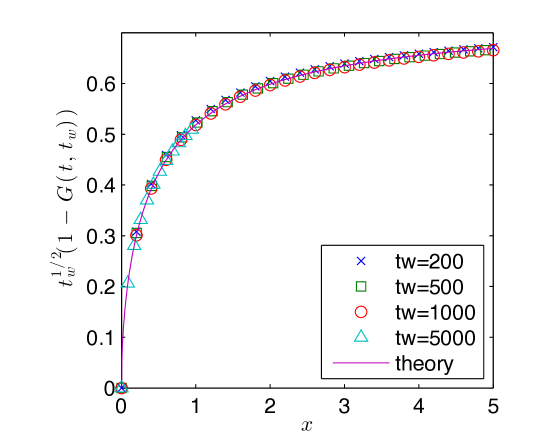
Figure 1: Scaling plot of stress relaxation function, showing the scaled decay of the stress relaxation function, $t_{\rm w}^{1/2}(1-G(t,t_{\rm w}))$, against $x=(t-t_{\rm w})/t_{\rm w}$. The system age $t_{\rm w}$ is as shown in the legend, and $t$ varies along each curve; $\alpha=0.3$. All data collapse onto a master curve proportional to $x^{1/2}/(1+x)^{1/2}$ as expected from our analysis in the long-time regime. The prefactor of the theoretical prediction is equal to $0.733$ and is determined as explained in Sec. 7.3.

For a systematic analysis in the long-time regime, which we perform in the following section, it is useful to rewrite (23) as

$$t_{\rm w}^{1/2}[1-G(t,t_{\rm w})]\sim\left(\frac{x}{1+x}\right)^{1/2}$$ (24)

where as previously $t=t_{\rm w}(1+x)$, i.e. $x=(t-t_{\rm w})/t_{\rm w}$. Our claim is then that in the limit of long times taken at constant $x$, $t_{\rm w}^{1/2}[1-G(t,t_{\rm w})]$ becomes a function of $x$ only. We show in Fig. 1 that this prediction is fully consistent with data obtained by direct numerical solution of the HL model, and is remarkably accurate even for a small waiting time $t_{\rm w}=200$.

5 Boundary layer analysis

5.1 Scaling forms

Based on the intuitive discussion above, we can write down suitable scaling forms for the solution $\delta p(\sigma,t)$ in the long-time regime, i.e. $t_{\rm w}\to\infty$ with $t=t_{\rm w}(1+x)$ and $x>0$ fixed. To shorten calculations we fix the scaling exponents directly from the insights in Sec. 4, rather than leaving them initially generic as we did for the unperturbed aging dynamics. The determination of the resulting scaling functions is the focus of this section.

In the interior, one expects

$$\delta p(\sigma,t)=\sum_{k\geq 0}t_{\rm w}^{-k/2}\left[\delta Q_{k}(\sigma,x)+B_{k}(\sigma t_{\rm w}^{1/2},x)+C_{k}((1-\sigma)t_{\rm w}^{1/2},x)\right]$$ (25)

where the $t_{\rm w}^{1/2}$ factors in $B_{k}$ and $C_{k}$ give the scale of the boundary layers arising from the diffusion; the width of the boundary layers on this scale will then grow with $x$ and eventually saturate. It is important to note that the size $\sim t_{\rm w}^{-1/2}$ of the boundary layers, which arises from diffusive dynamics, is significantly larger than in the unperturbed dynamics where it is $\sim t_{\rm w}^{-1}$.

In the exterior we expect, on the other hand,

$$\delta p(\sigma,t)=\sum_{k\geq 0}t_{\rm w}^{-k/2}\delta R_{k}((\sigma-1)t_{\rm w},x).$$ (26)

with boundary layer size $t_{\rm w}^{-1}$ inherited from the unperturbed solution. Note that for both the interior and exterior we have given the expressions as they apply for $\sigma>0$; the ones for $\sigma<0$ follow by anti-symmetry of $\delta p$.

We remark that the long-time limit considered here always has $t-t_{\rm w}$ large because we are keeping $x>0$ fixed. For time differences of order unity the scaling forms above do not apply: physically, they cannot describe the fast transient that brings the value of $\delta p(1,t)$ down to $\sim(t-t_{\rm w})^{-1/2}$. The limit of $t-t_{\rm w}\gg 1$ (but of order unity) should nevertheless match the $x\to 0$ limit of $t-t_{\rm w}=xt_{\rm w}$, and indeed we will find a scaling with $(t_{\rm w}x)^{-1/2}$ below for the leading order term in $\delta p(1,t)$.

5.2 Boundary and initial conditions

We next consider the boundary and initial conditions for the boundary layer functions $B_{k}$, $C_{k}$, $R_{k}$. Antisymmetry requires the boundary condition at zero

$$\delta Q_{k}(0,x)+B_{k}(0,x)=0$$ (27)

The boundary conditions from continuity at $\sigma=1$ are

$$\delta Q_{k}(1,x)+C_{k}(0,x)=\delta R_{k}(0,x)$$ (28)

and from continuity of the derivative

$$\partial_{\sigma}Q_{m}(1,x)-\partial_{z}C_{m+1}(0,x)=\partial_{z}\delta R_{m+2}(0,x)$$ (29)

The initial conditions for the interior boundary layers are that $B_{k}(z,x\to 0)=C_{k}(z,x\to 0)=0$ for $z>0$. The initial conditions for the $\delta Q_{k}$ follow from the fact that $\delta p(\sigma,t_{\rm w})=-\partial_{\sigma}p_{0}(\sigma,t_{\rm w})$. So if $p_{0}(\sigma,t_{\rm w})=\sum_{k}t_{\rm w}^{-k}Q_{k}(\sigma)$, then $\delta Q_{2k}(\sigma,0)=-\partial_{\sigma}Q_{k}(\sigma)$ while $\delta Q_{2k+1}(\sigma,0)=0$. The initial conditions for the $\delta R_{k}$ are more subtle but fortunately are not needed because these functions are adiabatically slaved to the interior as discussed below.

For the following analysis, in order to be able to use expansions in $t_{\rm w}^{-1/2}$ rather than $t_{\rm w}^{-1}$ throughout, we will also write the unperturbed diffusion rate as

$$D(t)=\sum_{l\geq 2}\tilde{d}_{l}t^{-l/2-1}=\sum_{l\geq 2}\tilde{d}_{l}t_{\rm w}^{-l/2-1}(x+1)^{-l/2-1}$$ (30)

with $\tilde{d}_{2k}=d_{k}$ and $\tilde{d}_{2k+1}=0$.

5.3 Determination of scaling functions

We can now write down the equations for the various scaling functions that follow from the linearized master equation (7). We assume that these functions decay quickly (faster than power law) when their first argument $z$ becomes large. In the interior $0<\sigma<1$ the boundary layers then do not contribute, so

$$\sum_{k\geq 0}t_{\rm w}^{-k/2-1}\partial_{x}\delta Q_{k}(\sigma,x)=\sum_{l\geq 2}\tilde{d}_{l}t_{\rm w}^{-l/2-1}(x+1)^{-l/2-1}\sum_{k\geq 0}t_{\rm w}^{-k/2}\partial_{\sigma}^{2}\delta Q_{k}(\sigma,x)$$ (31)

and therefore

$$\partial_{x}\delta Q_{m}(\sigma,x)=\sum_{l=2}^{m}\tilde{d}_{l}(x+1)^{-l/2-1}\partial_{\sigma}^{2}\delta Q_{m-l}(\sigma,x)$$ (32)

Because only even $l$ contribute to the sum, one sees that the even and odd $\delta Q_{m}$ decouple, and given that only even ones feature in the initial condition at $x=0$, the odd ones will vanish at all $x$. The leading order term is $\partial_{x}\delta Q_{0}=0$, so that $\delta Q_{0}(\sigma,x)=\delta Q_{0}(\sigma,0)$ is independent of the rescaled time difference $x$. Note that each higher-order $\delta Q_{m}$ is determined simply by integrating over $x$ a function of $\sigma$ and $x$ that is known from the lower orders. In particular one is not solving a diffusion equation here, so one does not need separate boundary conditions for the $\delta Q_{m}$ themselves. This is because the continuity at the boundaries is handled by the boundary layer functions $B_{k}$ and $C_{k}$.

In the interior near $\sigma=0$, i.e. for fixed $z=\sigma t_{\rm w}^{1/2}$ of order unity one gets from (7)

$$\sum_{k\geq 0}t_{\rm w}^{-k/2-1}\left[\sum_{n\geq 0}\frac{1}{n!}z^{n}t_{\rm w}^{-n/2}\partial_{\sigma}^{n}\partial_{x}\delta Q_{k}(0,x)+\partial_{x}B_{k}(z,x)\right]$$

$$= \sum_{l\geq 2}\tilde{d}_{l}t_{\rm w}^{-l/2-1}(x+1)^{-l/2-1}\sum_{k\geq 0}t_{\rm w}^{-k/2}\left[\sum_{n\geq 0}\frac{1}{n!}z^{n}t_{\rm w}^{-n/2}\partial_{\sigma}^{n+2}\delta Q_{k}(0,x)+t_{\rm w}\partial_{z}^{2}B_{k}(z,x)\right]$$

and so

$$\!\!\!\!\!\!\!\!\!\!\!\!\!\!\!\!\!\!\!\!\!\!\!\!\sum_{k=0}^{m}\frac{z^{m-k}}{(m-k)!}\partial_{\sigma}^{m-k}\partial_{x}\delta Q_{k}(0,x)+\partial_{x}B_{m}(z,x)\ =$$

$$= \sum_{l\geq 2}^{k+l}\sum_{k\geq 0}^{\leq m}\tilde{d}_{l}(x+1)^{-l/2-1}\frac{z^{m-k-l}}{(m-k-l)!}\partial_{\sigma}^{m-k-l+2}\delta Q_{k}(0,x)$$

$${}+\sum_{k=0}^{m}\tilde{d}_{m+2-k}(x+1)^{-(m-k)/2-2}\partial_{z}^{2}B_{k}(z,x)$$

The first term on the left hand side is, from the equation for $\delta Q_{m}$,

$$\sum_{k=0}^{m}\sum_{l=2}^{k}\tilde{d}_{l}(x+1)^{-l/2-1}\frac{z^{m-k}}{(m-k)!}\partial_{\sigma}^{m-k+2}\delta Q_{k-l}(0,x)$$ (35)

or with $k=k^{\prime}+l$

$$\sum_{l=2}^{m}\sum_{k^{\prime}=0}^{m-l}\tilde{d}_{l}(x+1)^{-l/2-1}\frac{z^{m-k^{\prime}-l}}{(m-k^{\prime}-l)!}\partial_{\sigma}^{m-k^{\prime}-l+2}\delta Q_{k^{\prime}}(0,x)$$ (36)

which is identical to the first term on the right. So we end up with

$$\partial_{x}B_{m}(z,x) = \sum_{k=0}^{m}\tilde{d}_{m+2-k}(x+1)^{-(m-k)/2-2}\partial_{z}^{2}B_{k}(z,x)$$ (37)

Again the odd and even terms decouple, and as for the odd ones the boundary condition (27) and the initial condition are zero, these functions will vanish. The even ones can be determined recursively, starting from $B_{0}$ which obeys

$$\partial_{x}B_{0}(z,x) = \tilde{d}_{2}(x+1)^{-2}\partial_{z}^{2}B_{0}(z,x)$$ (38)

and has boundary condition $B_{0}(0,x)=\delta Q_{0}(0,x)=\delta Q_{0}(0,0)$ and initial condition $B_{0}(z,x\to 0)=0$ for $z>0$. The solution of this is

$$B_{0}(z,x)=\delta Q_{0}(0,0)\left\{-1+\mbox{erf}(z/[2(\tilde{d}_{2}x/(1+x))^{1/2}])\right\}$$ (39)

Next we look at $\sigma$ close to 1, i.e. $z=(1-\sigma)t_{\rm w}^{1/2}$ finite. Then one derives from the master equation, exactly as for $\sigma$ close to zero, for the $C_{m}$ the equations

$$\partial_{x}C_{m}(z,x) = \sum_{k=0}^{m}\tilde{d}_{m+2-k}(x+1)^{-(m-k)/2-2}\partial_{z}^{2}C_{k}(z,x)$$ (40)

The difference to the $B_{m}$ is that to get the relevant boundary condition, we also need the solution on the other side of $\sigma=1$, i.e. the $\delta R_{k}$. For these one gets from the master equation and with $z=(\sigma-1)t_{\rm w}$

$$\sum_{k\geq 0}t_{\rm w}^{-k/2}t_{\rm w}^{-1}\partial_{x}\delta R_{k}(z,x) = \sum_{l\geq 2}\tilde{d}_{l}t_{\rm w}^{-l/2-1}(x+1)^{-l/2-1}\sum_{k\geq 0}t_{\rm w}^{-k/2}t_{\rm w}^{2}\partial_{z}^{2}\delta R_{k}(z,x)$$ (41)

$${}-\sum_{k\geq 0}t_{\rm w}^{-k/2}\delta R_{k}(z,x)$$

and so

$$\delta R_{m}(z,x) = -\partial_{x}\delta R_{m-2}(z,x)+\sum_{l\geq 2}\tilde{d}_{l}(x+1)^{-l/2-1}\partial_{z}^{2}\delta R_{m+2-l}(z,x)$$ (42)

The first three of these equations are

$$\delta R_{0}(z,x) = \tilde{d}_{2}(x+1)^{-2}\partial_{z}^{2}\delta R_{0}(z,x)$$ (43)

$$\delta R_{1}(z,x) = \tilde{d}_{2}(x+1)^{-2}\partial_{z}^{2}\delta R_{1}(z,x)$$ (44)

$$\delta R_{2}(z,x) = -\partial_{x}\delta R_{0}(z,x)+\tilde{d}_{2}(x+1)^{-2}\partial_{z}^{2}\delta R_{2}(z,x)+\tilde{d}_{4}(x+1)^{-3}\partial_{z}^{2}\delta R_{0}(z,x)$$ (45)

The time derivative ($\partial_{x}$) terms are always subleading, which is consistent with the idea that the tails of $\delta p$ are evolving essentially adiabatically. One can then proceed to solve order by order. The first equation is solved by

$$\delta R_{0}(z,x) = r_{0}(x)e^{-z(x+1)/\tilde{d}_{2}^{1/2}}$$ (46)

But the derivative boundary condition (29) tells us that $\partial_{z}R_{0}(0,x)=0$, which implies $r_{0}(x)=0$, i.e. $\delta R_{0}(z,x)=0$. Then the boundary condition (28) gives $\delta Q_{0}(1,x)+C_{0}(0,x)=0$, hence $C_{0}(0,x)=-\delta Q_{0}(1,x)=-\delta Q_{0}(1,0)$. We can now solve for $C_{0}$, which by analogy with $B_{0}$ becomes

$$C_{0}(z,x)=\delta Q_{0}(1,0)\left\{-1+\mbox{erf}(z/[2(\tilde{d}_{2}x/(1+x))^{1/2}])\right\}$$ (47)

The functional form of the dependence on $z$ is consistent with the qualitative discussion in Sec. 4, reflecting the fact that the stress dynamics for $\sigma<1$ is diffusive, with effectively an absorbing boundary at $\sigma=1$. At the next order, the solution for $\delta R_{1}$ has the form

$$\delta R_{1}(z,x) = r_{1}(x)e^{-z(x+1)/\tilde{d}_{2}^{1/2}}$$ (48)

The derivative boundary condition is

$$-\partial_{z}\delta R_{1}(0,x) = \partial_{z}C_{0}(0,x)\ =\ \delta Q_{0}(1,0)\frac{2}{\sqrt{\pi}[2(\tilde{d}_{2}x/(1+x))^{1/2}]}$$ (49)

This must equal $r_{1}(x)(x+1)\tilde{d}_{2}^{-1/2}$, which fixes $r_{1}(x)$ and so

$$\delta R_{1}(z,x) = \frac{\delta Q_{0}(1,0)}{\sqrt{\pi x(1+x)}}\,e^{-z(x+1)/\tilde{d}_{2}^{1/2}}$$ (50)

For small $x$ the amplitude of this scales as $x^{-1/2}$, and so the leading tail has overall amplitude $t_{\rm w}^{-1/2}x^{-1/2}=(t-t_{\rm w})^{-1/2}$, as argued above. The actual initial condition at $t=t_{\rm w}$ (which is not directly accessible by our long-time scaling with $x>0$ and then $t_{\rm w}\to\infty$) can be estimated by extrapolating to $t-t_{\rm w}$ of order unity, i.e. $x\sim 1/t_{\rm w}$, and one then finds as expected that the tail amplitude is initially of order unity.

As at the previous order, knowledge of $\delta R_{1}$ determines the boundary condition (28) $C_{1}(0,x)=\delta R_{1}(0,x)$ for $C_{1}$. The latter can then be found from

$$\partial_{x}C_{1}(z,x) = \tilde{d}_{2}(x+1)^{-2}\partial_{z}^{2}C_{1}(z,x)$$ (51)

where the explicit result involves typical diffusive quadratic exponentials of $z$, and $z\,\mbox{erfc}(\cdots z)$. This then gives the required boundary condition on $\delta R_{2}$, and one can continue to solve iteratively in this way.

5.4 Evaluation of the stress relaxation function

Using the scaling forms for $\delta p$ discussed in Sec. 5.1, the stress relaxation function $G(t,t_{\rm w})=2\int_{0}^{\infty}d\sigma\,\sigma\,p(\sigma,t)$ can be written in the form

$$G(t,t_{\rm w}) = \sum_{k\geq 0}t_{\rm w}^{-k/2}\Biggl{[}2\int_{0}^{1}d\sigma\,\sigma\,\delta Q_{k}(\sigma,x)+2t_{\rm w}^{-1}\int_{0}^{\infty}dz\,z\,B_{k}(z,x)$$

$${}+2t_{\rm w}^{-1/2}\int_{0}^{\infty}dz\,(1-zt_{\rm w}^{-1/2})C_{k}(z,x)\Biggr{]}$$

$${}+\sum_{k\geq 0}t_{\rm w}^{-k/2}t_{\rm w}^{-1}\int_{0}^{\infty}dz\,(1+zt_{\rm w}^{-1})\delta R_{k}(z,x)$$

From the fact that $\delta Q_{0}(\sigma,x)=\delta Q_{0}(\sigma,0)=-\partial_{\sigma}Q_{0}(\sigma)$ and that $Q_{0}(\sigma)$ must integrate to one between $\sigma=-1$ and $\sigma=1$, the first term in square brackets is unity. The only term that contributes to the leading order decay from this initial value is $C_{0}$, giving to this leading order

$$t_{\rm w}^{1/2}[1-G(t,t_{\rm w})] = -2\int_{0}^{\infty}dz\,C_{0}(z,x)$$ (53)

One can insert the explicit solution (47) to get

$$t_{\rm w}^{1/2}[1-G(t,t_{\rm w})] = 4\,\delta Q_{0}(1,0)\biggl{(}\frac{\tilde{d}_{2}}{\pi}\biggr{)}^{1/2}\left(\frac{x}{1+x}\right)^{1/2}$$ (54)

This depends on the frozen-in part of the aging solution via $\delta Q_{0}(1,0)=-\partial_{\sigma}Q_{0}(1)$ and via $\tilde{d}_{2}=d_{1}$. We have therefore established the result (24) obtained earlier from qualitative arguments, and identified the relevant, initial-condition dependent, prefactors.

6 Linear response to oscillatory strain

We now turn to the study of oscillatory shear. From the relaxation function $G$ one can obtain information on the response to oscillatory strain, $\gamma(t)\propto\mathrm{e}^{\mathrm{i}\omega t}$ (with the real part giving the physical strain). The stress response is of the form $\langle\sigma\rangle(t)=G^{*}(\omega)\gamma(t)$. In time-translation invariant systems, where the stress relaxation function $G(t,t_{\rm w})$ depends only on $t-t_{\rm w}$, the complex shear modulus or “viscoelastic spectrum” $G^{*}(\omega)$ is then proportional to the Fourier transform of $G$.

For aging fluids the situation is more subtle because time translation invariance is lost (see [9]). The most general description of the complex modulus is then as a function of the time $t_{\rm w}$ when the strain is switched on, of the frequency $\omega$ and of the time $t$ when the stress is measured:

$$G^{*}(\omega,t,t_{\rm w})=G(t,t_{\rm w})\mathrm{e}^{-\mathrm{i}\omega(t-t_{w})}+\mathrm{i}\omega\int_{t_{\rm w}}^{t}dt^{\prime}G(t,t^{\prime})\mathrm{e}^{-\mathrm{i}\omega(t-t^{\prime})}.$$ (55)

However in the long-time regime function $G^{*}$ may be close to the “forward spectrum” defined by

$$G^{*}(\omega,t)=\mathrm{i}\omega\int_{t}^{\infty}dt^{\prime}G(t^{\prime},t)\mathrm{e}^{-\mathrm{i}\omega(t^{\prime}-t)}.$$ (56)

which is calculated as if the strain was applied from $t$ into the future. Physically, the conditions for this approximation to hold are [9] that $\omega\ll 1$ (relaxation timescales are large for long time so we need to look at small frequencies), $\omega t_{\rm w}\gg 1$ (strain starts sufficiently late after initial preparation to make transient effects small) and $\omega(t-t_{\rm w})\gg 1$ (many cycles of strain are performed before a measurement is taken). We show in Appendix B that these expectations are indeed correct for the HL-model, by comparing the explicit expressions for $G^{*}(\omega,t,t_{\rm w})$ and $G^{*}(\omega,t)$ in the long-time limit.

We can thus focus on the forward spectrum. To evaluate this in the long-time limit, we insert $G(t^{\prime},t)=1-c(t^{-1/2}-t^{\prime-1/2})$ from (23) into (56), with $c=4\,\delta Q_{0}(1,0)({\tilde{d}_{2}}/{\pi})^{1/2}$ the prefactor identified in (54). Changing integration variable to $w^{\prime}=\omega(t^{\prime}-t)$ then gives

$$G^{*}(\omega,t)=1-\frac{c}{\sqrt{t}}\,\mathrm{i}\int_{0}^{\infty}dw^{\prime}\sqrt{\frac{w^{\prime}}{w+w^{\prime}}}\mathrm{e}^{-\mathrm{i}w^{\prime}}$$ (57)

with the scaled frequency $w=\omega t$. The integral can be expressed in terms of Hankel functions (see B) but in fact we only need to know its behaviour for large $w$ as that is the regime where the forward spectrum is physically meaningful. Here, anticipating that the integral is dominated by $w^{\prime}$ of order unity, we can approximate $[w^{\prime}/(w+w^{\prime})]^{1/2}\approx(w^{\prime}/w)^{1/2}$. The integral then becomes proportional to a Gamma function so that

$$G^{*}(\omega,t)\approx 1-\frac{c}{\sqrt{wt}}\frac{\mathrm{i}\sqrt{\pi}}{2\mathrm{i}^{3/2}}=1-(1-\mathrm{i})\frac{c\pi}{\sqrt{8wt}}$$ (58)

or for the real and imaginary part

$$G^{\prime}(\omega,t)\approx 1-\frac{c\pi}{\sqrt{8wt}}$$ (59)

$$G^{\prime\prime}(\omega,t)\approx\frac{c\pi}{\sqrt{8wt}}$$ (60)

In these expressions one can of course equivalently write $\sqrt{wt}=\sqrt{\omega}t$. The former version makes it clearer that $\sqrt{t}[1-G^{*}(\omega,t)]$ becomes a function of the scaling variable $w$ for large $t$. This conclusion is physically sensible, and mirrors the fact that $\sqrt{t_{\rm w}}[1-G(t,t_{\rm w})]$ becomes a function of $x=(t-t_{\rm w})/t_{\rm w}$ for long times: for conventional aging, where the amplitude of the decay of $G(t,t_{\rm w})$ is independent of $t_{\rm w}$, one would expect $G^{*}(\omega,t)$ itself to become a function of $w$. Here one needs to multiply $1-G^{*}$ by $\sqrt{t}$ to compensate for the $1/\sqrt{t}$ dependence of the decay amplitude.

7 Comparison with numerical results

We have already provided in Fig. 1 numerical data that clearly supports our main prediction (24) for the decay of the stress relaxation function. In this section we give a more detailed comparison with numerics, and in particular we validate the boundary layer scaling forms assumed in our analysis.

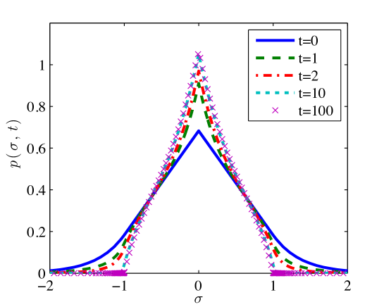
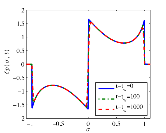
Figure 2: (a) Snapshots of numerical solution $p(\sigma,t)$ for times $t=0$, 1, 2, 10, 100. Note the progressive freezing in the interior range $-1<\sigma<1$ and the shrinking boundary layer in the exterior. (b) Snapshots of linear perturbation $\delta p(\sigma,t)$ due to step strain at time $t_{\rm w}=200$, for $t-t_{\rm w}=0$, $100$, $1000$. Here there is an additional boundary layer around $\sigma=0$.

We focus on a setting broadly representative of a “crunch”, i.e. sudden change in density of the material at time zero by compression. The initial stress distribution $p_{0}(\sigma,0)$ is chosen as the stationary solution of the HL-model [12] for the value $\alpha=1$, well outside the glass phase. The crunch at time zero is assumed to bring the system into the glassy regime at some $\alpha<1/2$ that then stays constant in time; we assume in particular $\alpha=0.3$. We then compute the numerical solution $p_{0}(\sigma,t)$ of (6) for this setting. For a series of waiting times $t_{\rm w}$ we also obtain $\delta p(\sigma,t)$ by solving (7) with initial condition (8), and finally compute $G(t,t_{\rm w})$ from (9). We give an overview of the numerical results for $p(\sigma,t)$ and $\delta p(\sigma,t)$ in Fig. 2.

7.1 Numerical methods

The numerical implementation of the above programme is not trivial: we need to use a discrete grid or “mesh” of $\sigma$-values; but as the solution of the problem develops boundary layers whose size decreases in time, also the mesh size needs to decrease to obtain accurate results.

Calculations were therefore performed with a combination of a (one-dimensional) finite-volume discretization of the PDE and a mesh refinement algorithm. Mesh refinement is based on a standard curvature estimate (see [19] for instance), taking into account that the diffusion coefficient of the linearized master equation (7) decays with time. While we cannot give quantitative error bounds for the accuracy of this approach, it certainly does refine at the locations where boundary layers are expected to appear. Small numerical artefacts are occasionally visible in the results, but usually only right before a refinement is made.

We have also carried out calculations with a constant mesh (using the most refined mesh obtained in a run with refinement but otherwise identical parameters), in order to separate the effects of mesh refinement from errors resulting from the discretization itself. The results of the two approaches are consistent with each other.

7.2 Aging without strain

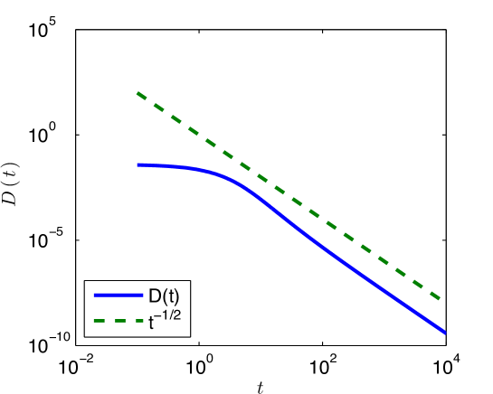
Figure 3: Log-log plot showing decay of diffusion constant $D(t)$ with time $t$for aging in the absence of strain. The asymptotic decay is $D\sim 1/t^{2}$ for long times, as indicated by the dashed line.

We first validate the scaling ansatz for $p(\sigma,t)$ around $\sigma=\pm 1$ and the time evolution of the diffusion constant. Starting with the latter, Fig. 3 shows that the theoretical expectation $D(t)\sim 1/t^{2}$ is well satisfied for long times, though reasonably large $t\approx 10^{2}$ are needed to clearly see this asymptotic regime Using the value of $D(t)$ at the largest time in our numerics, we estimate the asymptotic prefactor in $D(t)\approx\tilde{d}_{2}/t^{2}$ as Convergence to a constant for large $t$ seems clear but as we can see, this convergence is, at least in this test case, very late. One must wait at least before one can consider the asymptotic regime to be attained. By using the last computed value to approximate $d_{2}$, one

$$\tilde{d}_{2}\approx 0.03804$$ (61)

For later use we note the corresponding value $1/\tilde{d}_{2}^{1/2}\approx 5.127$.

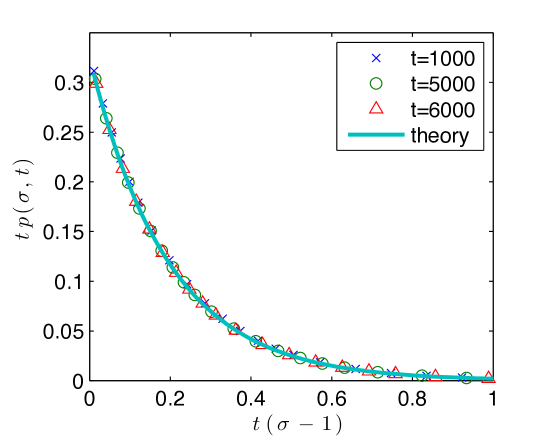
Figure 4: Scaling plot of exterior tail behaviour for aging without strain, showing $tp(\sigma,t)$ versus $z=t(\sigma-1)$ for $t=1000,5000,6000$ The bold line gives the theoretical prediction $[\tilde{d}_{2}^{1/2}/(2\alpha)]\exp(-z/\tilde{d}_{2}^{1/2})$ with $\tilde{d}_{2}$ given by (61).

We can verify our theoretical approach in more detail by studying the tail behaviour of $p(\sigma,t)$ around $\sigma=1$. According to Eq. (50) this is

$$p(t,\sigma)\approx\frac{\tilde{d}_{2}^{1/2}}{2\alpha}\,\frac{1}{t}e^{-t(\sigma-1)/\tilde{d}_{2}^{1/2}}$$ (62)

to leading order for large $t$. This means that plots of $tp(t,\sigma)$ against $z=t(\sigma-1)$ for different $t$ should collapse onto the master curve $[\tilde{d}_{2}^{1/2}/(2\alpha)]\exp(-z/\tilde{d}_{2}^{1/2})$. We demonstrate this in Figure 4, using the value for $1/\tilde{d}_{2}^{1/2}$ estimated from the diffusion constant data. Consistency with the theory can also be checked in the other direction: a plot of $\ln[tp(\sigma,t)]$ against $z$ should be a straight line of slope $1/\tilde{d}_{2}^{1/2}$. Performing such a fit gives $1/d_{2}^{1/2}\approx 5.125$ in good agreement with the value (61) from the diffusion data.

7.3 Linear response

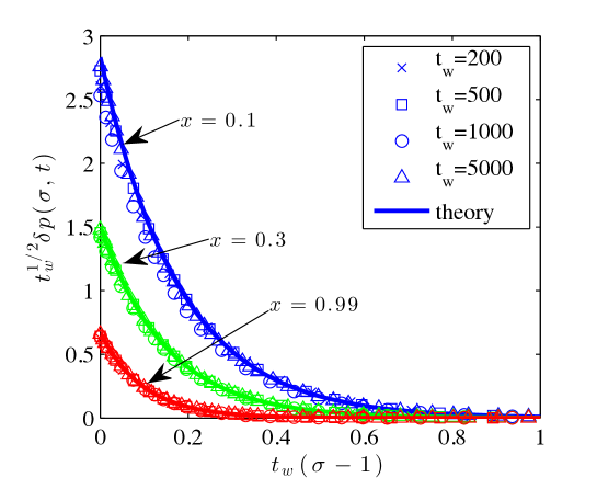
Figure 5: Decay of the linear perturbation solution $\delta p(\sigma,t)$ in the exterior boundary layer. Shown is $t_{\rm w}^{1/2}\delta p(\sigma,t)$ versus $t_{\rm w}(\sigma-1)$ for different $x=(t-t_{\rm w})/t_{\rm w})$ – as indicated by the arrows and respective colours – and different $t_{\rm w}$ as shown by the symbols. Solid lines give the prediction from the scaling theory for $t_{\rm w}\to\infty$.

We next consider the behaviour of the linear response $\delta p(\sigma,t)$. We begin with the exterior tail ($\sigma>1$.) To leading order for large times, our scaling theory predicts for this

$$\delta p(\sigma,t)\approx\frac{1}{\sqrt{t_{\rm w}}}\frac{\delta Q_{0}(1,0)}{\sqrt{\pi x(1+x)}}\,e^{-t_{\rm w}(\sigma-1)(x+1)/\tilde{d}_{2}^{1/2}}$$ (63)

To verify this, we plot $t_{\rm w}^{-1/2}\delta p(\sigma,t)$ versus $t_{\rm w}(\sigma-1)$ in Fig. 5 for several different values of $x$. The data are clearly consistent with the scaling prediction, with deviations that are surprisingly small even when $t-t_{\rm w}$ is not very large (i.e. for small $x$ and $t_{\rm w}$; for $x=0.1$ and $t_{\rm w}=200$ one has $t-t_{\rm w}=20$). For the prefactor of the theoretical prediction we need to estimate the prefactor $\delta Q_{0}(1,0)=-\partial_{\sigma}Q_{0}(\sigma=1)$. We do this by taking the numerical derivative of $p_{0}$, at the largest time available in our numerics since $p_{0}(\sigma,t)=Q_{0}(\sigma)+O(1/t)$. Note that the resulting estimate of $\delta Q_{0}(1,0)\approx 1.666$ is also used in determining the prefactor $4\delta Q_{0}(1,0)(\tilde{d}_{2}/\pi)^{1/2}$ of the theoretical prediction shown in Fig. 1.

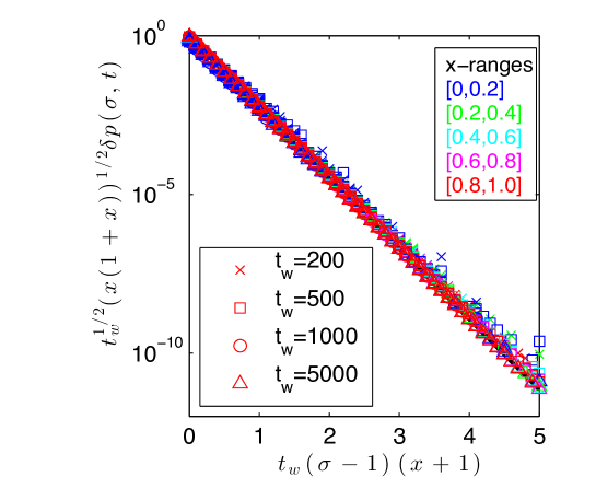
Figure 6: Master curve for tail behaviour of the linear perturbation solution $\delta p(\sigma,t)$. Shown is $t_{\rm w}^{1/2}[x(1+x)]^{1/2}\delta p(\sigma,t)$ versus $t_{\rm w}(\sigma-1)(x+1)$ for a range of different $x=(t-t_{\rm w})/t_{\rm w}$ and $t_{\rm w}$. The value of $t_{\rm w}$ is indicated by the symbol used, as in Fig. 5. Colours identify the range of $x$ as shown in the legend. Black solid line: prediction from the scaling theory.

To check the results for a broader range of $x$, we plot in Fig. 6 $[\pi x(1+x)]^{1/2}t_{\rm w}^{1/2}\delta p(\sigma,t)$ on a logarithmic axis against $t_{w}(\sigma-1)(x+1)=t(\sigma-1)$. This plot should be a straight line from (63), and again the data closely follow this prediction. Deviations become visible only for small $x$ and $t_{\rm w}$, and primarily in the regime where the scaled $\delta p$ is already very small. As before one can check consistency in the reverse direction also, by fitting the slope of the straight line in Fig. 6. This produces the estimate $1/d_{2}^{1/2}\approx 5.132$, again in good agreement with the value (61) estimated from the diffusion data.

Next we consider the behaviour $\delta p(\sigma,t)$ in the interior $-1<\sigma<1$ where it is a little more complex. We want to confirm in particular that the boundary layer sizes scale as $t_{\rm w}^{-1/2}$ rather than as $t_{\rm w}^{-1}$ in the exterior. In the interior there are two boundary layers, around $\sigma=0$, and $\sigma=1$ (with a mirror image around $\sigma=-1$. As the scaling is the same except for prefactors – compare (39) and (47) – we focus on $\sigma=1$. From the theory we have here to leading order

$$\delta p(\sigma,t)\approx\delta Q_{0}(\sigma,0)+\delta Q_{0}(1,0)\left\{-1+\mbox{erf}(z/[2(\tilde{d}_{2}x/(1+x))^{1/2}])\right\}.$$ (64)

where now $z=(1-\sigma)t_{\rm w}^{1/2}$. The first term, $\delta Q_{0}(\sigma,0)$, depends on the preparation of the system and so is not known a priori. But it drops out if we consider $\delta p(\sigma,t_{\rm w})-\delta p(\sigma,t)$. We plot this quantity against $(1-\sigma)t_{\rm w}^{1/2}$ in Fig. 7 for three values of $x$ and several values of $t_{\rm w}$, in analogy to Fig. 5 for the exterior boundary layer. In Fig. 8 we show the master curve of $\delta p(\sigma,t_{\rm w})-\delta p(\sigma,t)$ against $(1-\sigma)t_{\rm w}^{1/2}[(x+1)/x]^{1/2}$ for several values of $x$ and $t_{\rm w}$. Note that since $\delta p(\cdot,t_{\rm w})$ is not computed on the same mesh as $\delta p(\cdot,t)$, we used linear interpolation to estimate $\delta p(\cdot,t_{\rm w})$ on the finer mesh.

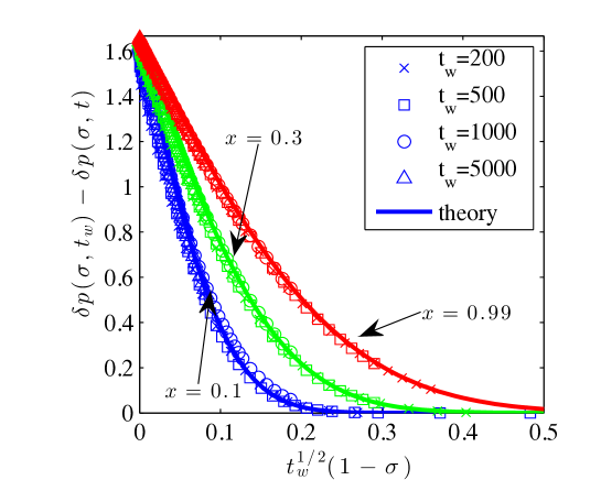
Figure 7: Behaviour of the linear perturbation solution $\delta p(\sigma,t)$ in the interior boundary layer at $\sigma=1$. Shown is $\delta p(\sigma,t_{\rm w})-\delta p(\sigma,t)$ versus $t_{\rm w}^{1/2}(1-\sigma)$ for different $x=(t-t_{\rm w})/t_{\rm w}$ – as indicated by the arrows and respective colours – and different $t_{\rm w}$ as shown by the symbols. Solid lines give the prediction from the scaling theory for $t_{\rm w}\to\infty$.

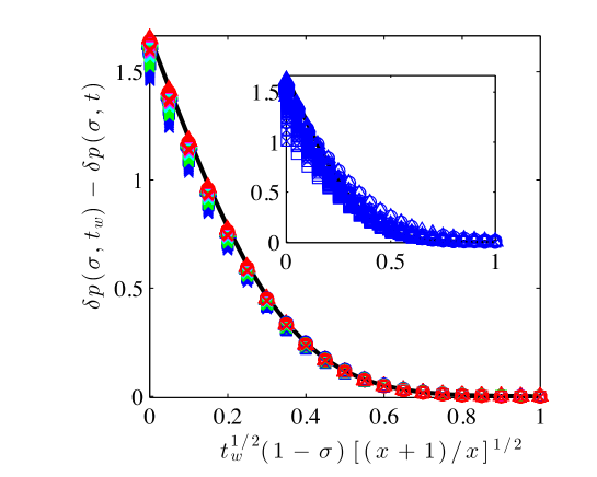
Figure 8: Master curve for the behaviour of the linear perturbation solution $\delta p(\sigma,t)$ in the interior boundary layer at $\sigma=1$. Shown is $\delta p(\sigma,t_{w})-\delta p(\sigma,t)$ versus $t_{\rm w}^{1/2}(1-\sigma)[(x+1)/x]^{1/2}$ for a range of different $x=(t-t_{\rm w})/t_{\rm w}$. Symbols and colors have the same meaning as in Fig. 6. Main plot shows values of $x>0.1$ while inset shows values of $x<0.1$.

8 Summary and outlook

We have studied the aging dynamics of the Hébraud-Lequeux (HL) model for the flow of amorphous materials, and the linear stress response to applied shear strain that it produces. Physically, the main qualitative conclusion is that the HL model in its glass phase freezes in a manner that depends on its initial preparation. This is because the diffusion constant $D(t)$ that drives stress relaxation decays so quickly that only a finite amount of memory of the initial condition can be erased. Accordingly the two-time stress relaxation function $G(t,t_{\rm w})$ does not decay fully even for $t\to\infty$, and its plateau value increases as the system becomes more elastic with in creasing age $t_{\rm w}$. The explicit result, from (23), is $G(t,t_{\rm w})=1-\mbox{const}\times(1/t_{\rm w}-1/t)^{1/2}$.

The same physics of course drives the response to oscillatory strain as measured by the viscoelastic spectrum. In the relevant limit of low frequencies $\omega$ and long measurement times $t$ we found that this behaves as $G^{*}(\omega,t)=1-\mbox{const}\times(1-i)/[t\sqrt{\omega}$. While the standard expectation for a system with simple aging would be a function depending on $\omega t$ only, here the deviation from purely elastic behaviour is not simply $1/\sqrt{\omega t}$, but is suppressed by an additional factor of $1/\sqrt{t}$.

Mathematically, what is interesting is that the HL requires rather different tools of analysis for its aging dynamics than e.g. for models such as SGR [8], where one can use temporal Laplace transforms and characteristics. In the HL case, most of the physics happens around the stress threshold ($=1$) above which yielding occurs. This necessitates the use of boundary layer techniques that have previously been deployed by one of us to understand the glass transtion in the HL model [17, 16, 18].

We saw that the boundary layer scaling with age $t_{\rm w}$ is different below and above the stress treshold in the linear response $\delta p(\sigma,t)$ of the stress distribution to step strain. In effect, yielding above the treshold is sufficiently fast for the stress relaxation to become dominated by diffusion of stress values $\sigma$ from below to just above the threshold, where yielding takes place effectively instantaneously.

Returning finally to the physical implication of our results, it seems to us that there is little evidence in experimental data on soft amorphous materials for the incompletely decaying stress relaxation $G(t,t_{\rm w})$ – and the increasing height of its plateau with age $t_{\rm w}$ – that we found for the HL-model in its aging phase. As the model has been widely used, also as a mean field description for spatially resolved model variants, it is important to be aware of this limitation. The insight that the freezing behaviour arises from a lack of “self-sustaining” noise in the model – as reflected in the rapid decay of $D(t)$ – may also help to develop more sophisticated variants of the model (e.g. [20]).

Appendix A Aging without strain

In this Appendix we study the equations for the aging dynamics, (16) and (18) with boundary conditions (19,20). Our aim is to find the exponent parameters $l$ and $s$, and from these determine the leading behaviour of $p(\sigma,t)$ summarized in (21,22). We show first, via several intermediate steps, that $l\leq s\leq 2l-1$. Assuming then a generic initial condition we further show that $l=s$, and argue that in fact $l=s=1$. The method will centre around determining for which $k$ the exterior functions $R_{k}^{\pm}(z)$ and the coefficients $d_{k}$ can be zero or non-zero.

A.1 General arguments

Starting with the $d_{k}$, define $n$ as

$$n=\min\{k|d_{k}\neq 0\},$$ (65)

Then in the sum in (18) the largest value of $k$ that contributes is $m+l-n$:

$$-\frac{m-s}{s}R^{\pm}_{m-s}+\frac{l}{s}zR^{\pm^{\prime}}_{m-s}=\sum_{k=0}^{m+l-n}d_{m-k+l}R^{\pm}_{k}{}^{\prime\prime}-R^{\pm}_{m}$$ (66)

We can deduce from this that $n=l$, proceeding by contradiction.

If $n>l$, then the term of the largest order (containing the $R^{\pm}_{k}$ with the largest $k$) is the last one on the r.h.s. of (66). Setting $m=0$ gives then $R^{\pm}_{0}=0$, and inductively one sees that all $R^{\pm}_{k}=0$, in contradiction to $d_{n}\neq 0$. Conversely, if $n<l$, then the term of the largest order is the $k=m+l-n$ contribution from the sum. Setting $m=n-l$ then gives $d_{n}R^{\pm}_{0}{}^{\prime\prime}=0$ and hence $R^{\pm}_{0}=0$, and inductively $R^{\pm}_{k}=0$, leading again to a contradiction. Having excluded both $n>l$ and $n<l$ proves that $n=l$, and so

$$d_{0}=\ldots=d_{l-1}=0.$$ (67)

Our next step is to deduce that also $R^{\pm}_{k}=0$ for $k=0,\ldots,l-1$, and to find the first nonzero function, $R^{\pm}_{l}$. Choosing $m=0$ in (66) yields

$$0=d_{l}R^{\pm}_{0}{}^{\prime\prime}-R^{\pm}_{0}$$ (68)

Now $d_{l}$ as the leading term in $D(t)$ has to be positive, hence (bearing in mind also the definition of $d^{\pm}_{0}$) one has $R^{\pm}_{0}=d^{\pm}_{0}/(\alpha\sqrt{d_{l}})\exp(-z/\sqrt{d_{l}})$. Since $R^{\pm}_{0}$ gives the leading contribution to $p(\sigma,t)$ in the exterior, it has to be non-negative, hence $d^{\pm}_{0}\geq 0$. But $d_{0}=d_{0}^{+}+d_{0}^{-}=0$ (from (67) together with $l\geq 1$), so we have $d^{\pm}_{0}=0$ and therefore $R^{\pm}_{0}=0$. Repeating the argument, one proves inductively that

$$R^{\pm}_{0}=\ldots=R^{\pm}_{l-1}=0$$ (69)

The first nonzero functions $R^{\pm}_{k}$ are then

$$R^{\pm}_{l}=\frac{d^{\pm}_{l}}{\alpha\sqrt{d_{l}}}e^{-z/\sqrt{d_{l}}}$$ (70)

Next we look at the interior profiles $Q_{k}$. We show that $s\leq 2l-1$; that the $Q_{k}$ vanish for $k=1,\ldots,2l-s-1$; and that $Q_{2l-s}$ has to be nonzero. We start from (16) and note that because of (67), the largest $k$ that can contribute in the sum is the one where $m-k-l=l$, i.e. $k=m-2l$:

$$-\frac{m-s}{s}Q_{m-s}=\sum_{k=0}^{m-2l}d_{m-k-l}Q^{\prime\prime}_{k}+d_{m-l}\frac{\delta(\sigma)}{\alpha}$$ (71)

Now if we had $s\geq 2l$, we could choose $m=2l$ and the l.h.s. would be zero (either because of the prefactor, for $s=2l$, or because $m-s<0$ so that $Q_{m-s}$ vanishes). This would give, after division by $d_{l}>0$,

$$0=Q^{\prime\prime}_{0}+\frac{\delta(\sigma)}{\alpha}$$ (72)

The solution of this equation would consist of two line segments, one for each of the regions $-1<\sigma<0$ and $0<\sigma<1$, but it is easy to show that in the glassy regime ($\alpha<1/2$) this solution would violate either positivity ($Q_{0}(\sigma)\geq 0$) or normalization ($\int_{-1}^{1}d\sigma\ Q_{0}(\sigma)=1$). The assumption $s\geq 2l$ has led to a contradiction, hence $s\leq 2l-1$ as announced.

Choosing successively $m=s+1,\ldots,2l-1$ in (71) then shows that

$$Q_{1}=\ldots=Q_{2l-s-1}=0$$ (73)

provided that $s\leq 2l-2$, otherwise there are no $m$ in the required range. On the other hand we have shown in (70) that at least one of the functions $R^{\pm}_{l}$ has to be nonzero, hence from the boundary condition (19) also $Q_{l}$ cannot be identically zero. Comparing with (73) yields $l\geq(2l-s-1)+1$, hence $s\geq l$. Overall, we have now deduced that $l\leq s\leq 2l-1$.

To get the first non-vanishing interior profile we set $m=2l$ in (71) to find

$$-\frac{2l-s}{s}Q_{2l-s}=d_{l}Q^{\prime\prime}_{0}+d_{l}\frac{\delta(\sigma)}{\alpha}$$ (74)

$Q_{2l-s}$ cannot vanish identically as otherwise we would get back to our previous equation (72) for $Q_{0}$ that has no valid solution. Instead we can use (74) to determine $Q_{2l-s}$ from $Q_{0}$, and then recursively $Q_{2l-s+1}$, $Q_{2l-s+2},\ldots$ for $m=2l+1,2l+2,\ldots$ What is notable is that we never get a closed equation for $Q_{0}$, which means that this profile must depend on the initial conditions.

A.2 Generic initial conditions lead to $l=s$

Consider now the generic case where one expects that the second derivatives $Q^{\prime\prime}_{0}(\pm 1)$ will not both vanish. Then one of $Q_{2l-s}(\pm 1)$ is nonzero from (74), and from (19) also the corresponding $R^{\pm}_{2l-s}(0)$ cannot vanish identically. But we know from (69) that all $R^{\pm}_{k}$ up to $k=l-1$ vanish, so $2l-s\geq l$, i.e. $l\geq s$. Together with $l\leq s$ as shown in the previous subsection, we therefore have in the generic case $l=s$.

One can show further that the $Q_{k}$ and $R^{\pm}_{k}$ vanish when $k$ is not a multiple of $s$, so that without loss of generality one can take $l=s=1$. These values imply that the boundary layer has width $1/t$, and the diffusion constant scales as $D\sim t^{-2}$ to leading order. This is consistent with initial condition-dependent freezing, because $\int D(t)dt<\infty$.

With $l=s=1$, the leading order equations are now

$$R^{\pm}_{1}(z) = \frac{d^{\pm}_{1}}{\alpha\sqrt{d_{1}}}e^{-z/\sqrt{d_{1}}}$$ (75)

$$-Q_{1}(\sigma) = d_{1}Q^{\prime\prime}_{0}(\sigma)+d_{1}\frac{\delta(\sigma)}{\alpha}$$ (76)

$$R^{\pm}_{1}(0) = \frac{d^{\pm}_{1}}{\alpha\sqrt{d_{1}}}\ =\ Q_{1}(\pm 1)\ =\ -d_{1}Q^{\prime\prime}_{0}(\pm 1)$$ (77)

$$R^{\pm}_{1}{}^{\prime}(0) = -\frac{d^{\pm}_{1}}{\alpha d_{1}}\ =\ \pm Q_{0}^{\prime}(\pm 1)$$ (78)

Recalling that $d_{1}=d_{1}^{+}+d_{1}^{-}$, the last line (78) gives

$$-Q_{0}^{\prime}(1)+Q_{0}^{\prime}(-1)=1/\alpha$$ (79)

This is a condition that the frozen profile needs to satisfy: here we have an aspect of $Q_{0}(\sigma)$ that is controlled by the aging dynamics with its partial loss of memory, rather than frozen-in initial information.

The result (77) shows that the frozen profile also has to have non-positive $Q_{0}^{\prime\prime}(\pm 1)$. Quantitatively, starting from (77), dividing by $\sqrt{d_{1}}$ and adding the two cases one has $-\sqrt{d_{1}}[Q_{0}^{\prime\prime}(1)+Q_{0}^{\prime\prime}(-1)]=1/\alpha$ and so

$$d_{1}=(-\alpha[Q_{0}^{\prime\prime}(1)+Q_{0}^{\prime\prime}(-1)])^{-2}$$ (80)

From (77) one then finds in more detail

$$d^{\pm}_{1}=\frac{-\alpha Q_{0}^{\prime\prime}(\pm 1)}{(-\alpha[Q_{0}^{\prime\prime}(1)+Q_{0}^{\prime\prime}(-1)])^{3}}.$$ (81)

These explicit expressions together with (75,76) demonstrate that up to order $1/t$ ($k=1$), all profiles $Q_{1}$, $R^{\pm}_{1}$ are fully determined by $Q_{0}^{\prime\prime}$.

A.3 Non-generic case

We comment briefly on the non-generic case where $Q_{0}^{\prime\prime}(\pm 1)=0$. Then $Q_{2l-s}(\sigma)$, which we already know does not vanish identically, is nonetheless zero for $\sigma=\pm 1$. The boundary condition (19) now implies that $R^{\pm}_{2l-s}(0)=0$, whereas at least one of $R^{+}_{l}(0)$ and $R^{-}_{l}(0)$ is nonzero from (70). Hence $l\geq 2l-s+1$ or $s\geq l+1$, which means that the width $\sim t^{-l/s}$ of the boundary layer is larger than in the generic case, decaying more slowly with time. We already know that $l\leq s\leq 2l-1$, so the smallest $l$ possible in the non-generic case is $l=2$, which would then imply $s=3$.

One can now ask about the next order in $Q_{k}$ beyond $k=2l-s$. Choosing $m=2l+1$ in (71) gives

$$-\frac{2l+1-s}{s}Q_{2l+1-s}=d_{l+1}Q^{\prime\prime}_{0}+d_{l}Q^{\prime\prime}_{1}+d_{l+1}\frac{\delta(\sigma)}{\alpha}$$ (82)

If $s=2l-1$, which is true for e.g. the choice $(l=2,s=3)$, then $Q_{1}$ obeys

$$-\frac{1}{s}Q_{1}=d_{l}Q_{0}^{\prime\prime}+d_{l}\frac{\delta(\sigma)}{\alpha}$$ (83)

from (74) and does not vanish identically. Inserting into (82) shows that $Q_{2l+1-s}\equiv Q_{2}$ then behaves as $Q^{\prime\prime}_{2}(\pm 1)\propto Q_{1}^{\prime\prime}(\pm 1)\propto Q_{0}^{(4)}(\pm 1)$ at the boundary. This suggests a further case division depending on whether these fourth derivatives both vanish, and there is likely to be a hierarchy of such further divisions depending on derivatives of increasing order of $Q_{0}(\sigma)$ at the boundaries. If at least one of the fourth derivatives is nonzero, then one of $Q_{2}(\pm 1)$ is also nonzero, hence from (19) so is one of $R_{2}^{\pm}(0)$. This implies $l\leq 2$, hence in fact $l=2$ because as shown above smaller $l$ are impossible in the non-generic case.

Above we had assumed $s=2l-1$, and we would conjecture that the opposite case $s\leq 2l-2$ can be excluded using similar arguments as in generic case. We will not explore this issue further here, however, as the non-generic case is unlikely to be relevant for physically plausibe initial conditions.

Appendix B Calculations for complex shear modulus

We first show that in the HL model the waiting-time dependent oscillatory shear modulus and the forward shear modulus become identical in the long-time limit.

To find an expression for the full $t_{\rm w}$-dependent shear modulus (55), we insert the expression (54) for the stress relaxation function $G(t,t_{\rm w})$ in the long time regime. We set $w=\omega t$, $w^{\prime}=\omega(t-t^{\prime})$ and recall that $x=(t-t_{\rm w})/t_{\rm w}$. One obtains with a few lines of algebra

$$G^{*}(\omega,t,t_{\rm w})=1-\frac{c}{\sqrt{t}}\left(\sqrt{x}\mathrm{e}^{-\mathrm{i}w(1-r)}+\mathrm{i}\int_{0}^{wx/(1+x)}dw^{\prime}\,\sqrt{\frac{w^{\prime}}{w-w^{\prime}}}\mathrm{e}^{-\mathrm{i}w^{\prime}}\right)$$ (84)

The term in brackets can be written as

$$\mathrm{i}\int dw^{\prime}f_{w,x}(w^{\prime})\mathrm{e}^{-\mathrm{i}w^{\prime}}$$ (85)

where

$$f_{w,x}(w^{\prime}) =\sqrt{\frac{w^{\prime}}{w-w^{\prime}}}\qquad \mbox{for}\quad w^{\prime}<wx/(1+x)$$ (86)

$$f_{w,x}(w^{\prime}) =\sqrt{x}\qquad \mbox{for}\quad w^{\prime}>wx/(1+x)$$ (87)

On the other hand the forward spectrum can be written in the long-time limit as (57):

$$G^{*}(\omega,t)=1-\frac{c}{\sqrt{t}}\,\mathrm{i}\int_{0}^{\infty}dw^{\prime}\sqrt{\frac{w^{\prime}}{w+w^{\prime}}}\mathrm{e}^{-\mathrm{i}w^{\prime}}$$ (88)

One now sees that for any fixed $w^{\prime}$, the two integrands become identical, both approaching $\sqrt{w^{\prime}/w}$, provided that $w$ and $wx/(1+x)$ are large (and in particular larger than $w^{\prime}$). So in this limit the full $t_{\rm w}$-dependent spectrum and the forward spectrum do indeed become identical.

Let us now compute the forward spectrum by computing the integral in (88). For the intermediate calculations it is convenient to express the dependence on $w$ in terms of $z=w/2$. We perform two changes of variables to carry out the integration over $w^{\prime}$. First we put $z^{\prime}=w^{\prime}/z+1$. This leads to the equality

$$\int_{0}^{\infty}dw^{\prime}\,\mathrm{e}^{-\mathrm{i}w^{\prime}}\sqrt{\frac{w^{\prime}}{w+w^{\prime}}} =z\mathrm{e}^{\mathrm{i}z}\int_{1}^{\infty}dz^{\prime}\,\mathrm{e}^{-\mathrm{i}zz^{\prime}}\sqrt{\frac{z^{\prime}-1}{z^{\prime}+1}}$$ (89)

Now set $z^{\prime}=\cosh(t)$ and use the hyperbolic trigonometric relations $\cosh(t)-1=2\sinh^{2}(t/2)$, $\cosh(t)+1=2\cosh^{2}(t/2)$ and

$$dz^{\prime} = \sinh(t)dt=2\sinh(t/2)\cosh(t/2)dt$$ (90)

Thus we find for our integral

$$=z\mathrm{e}^{\mathrm{i}z}\int_{0}^{\infty}dt\,\mathrm{e}^{-\mathrm{i}z\cosh(t)}\sqrt{\frac{2\sinh^{2}(t/2)}{2\cosh^{2}(t/2)}}2\sinh(t/2)\cosh(t/2)$$ (91)

$$=2z\mathrm{e}^{\mathrm{i}z}\int_{0}^{\infty}dt\,\mathrm{e}^{-\mathrm{i}z\cosh(t)}\sinh^{2}(t/2)$$ (92)

$$=z\mathrm{e}^{\mathrm{i}z}\int_{0}^{\infty}dt\,\mathrm{e}^{-\mathrm{i}z\cosh(t)}(\cosh(t)-1)$$ (93)

The remaining integral can be expressed in terms of Hankel functions [21] defined as:

$$H_{\nu}^{(2)}(z)=-2\frac{\mathrm{e}^{\mathrm{i}\nu\pi/2}}{\pi}\int_{0}^{\infty}\mathrm{e}^{-\mathrm{i}z\cosh(t)}\cosh(\nu t)dt$$ (94)

This gives eventually

$$G^{*}(w,t)=1+\frac{c\pi}{4\sqrt{t}}w\mathrm{e}^{\mathrm{i}w/2}\left(H_{0}^{(2)}(w/2)+\mathrm{i}H_{1}^{(2)}(w/2)\right)$$ (95)

From asymptotic properties of the Hankel functions, one can then obtain for $w\gg 1$ the expression (58) in the main text.

References

- [1] D Rodney, A Tanguy, and D Vandembroucq. Modeling the mechanics of amorphous solids at different length scale and time scale. Modelling and Simulation in Materials Science and Engineering, 19:083001, 2011.
- [2] D T N Chen, Q Wen, P A Janmey, J C Crocker, and A G Yodh. Rheology of soft materials. Annual Review of Condensed Matter Physics, Vol 1, 1:301–322, 2010.
- [3] P Coussot. Rheophysics of pastes: a review of microscopic modelling approaches. Soft Matter, 3(5):528–540, 2007.
- [4] M L Falk and J S Langer. Dynamics of viscoplastic deformation in amorphous solids. Phys. Rev. E, 57(6):7192–7205, 1998.
- [5] M L Falk and J S Langer. Deformation and failure of amorphous, solidlike materials. Ann. Rev. Cond. Matt. Phys., Vol 2, 2:353–373, 2011.
- [6] J S Langer. Shear-transformation-zone theory of yielding in athermal amorphous materials. Physical Review E, 92:012318, 2015.
- [7] P Sollich, F Lequeux, P Hébraud, and M E Cates. Rheology of soft glassy materials. Phys. Rev. Lett., 78:2020–2023, 1997.
- [8] P Sollich. Rheological constitutive equation for a model of soft glassy materials. Phys. Rev. E, 58:738–759, 1998.
- [9] S M Fielding, P Sollich, and M E Cates. Aging and rheology in soft materials. J. Rheol., 44(2):323–369, 2000.
- [10] P Sollich and M E Cates. Thermodynamic interpretation of soft glassy rheology models. Phys. Rev. E, 85:031127, 2012.
- [11] F Da Cruz, F Chevoir, D Bonn, and P Coussot. Viscosity bifurcation in granular materials, foams, and emulsions. Phys. Rev. E, 66:051305, 2002.
- [12] P Hébraud and F Lequeux. Mode-coupling theory for the pasty rheology of soft glassy materials. Phys. Rev. Lett., 81(14):2934–2937, 1998.
- [13] L Bocquet, A Colin, and A Ajdari. Kinetic theory of plastic flow in soft glassy materials. Phys. Rev. Lett., 103:036001, 2009.
- [14] V Mansard, A Colin, P Chauduri, and L Bocquet. A kinetic elasto-plastic model exhibiting viscosity bifurcation in soft glassy materials. Soft Matter, 7(12):5524–5527, 2011.
- [15] A Nicolas, K Martens, L Bocquet, and J L Barrat. Universal and non-universal features in coarse-grained models of flow in disordered solids. Soft Matter, 10(26):4648–4661, 2014.
- [16] Julien Olivier and Michael Renardy. Glass transition seen through asymptotic expansions. SIAM J. Appl. Math., 71(4):1144–1167, 2011.
- [17] Julien Olivier. Asymptotic analysis in flow curves for a model of soft glassy rheology. Z. Angew. Math. Phys, 61(3):445–466, 2010.
- [18] Julien Olivier and Michael Renardy. On the generalization of the Hébraud-Lequeux model to multidimensional flows. Arch. Ration. Mech. Anal., 208(2):569–601, 2013.
- [19] Weizhang Huang and Robert D Russell. Adaptive Moving Mesh Methods, volume 174 of Applied Mathematical Science. Springer, 2011.
- [20] J P Bouchaud, S Gualdi, M Tarzia, and F Zamponi. Spontaneous instabilities and stick-slip motion in a generalized Hébraud-Lequeux model. Soft Matter, 12(4):1230–1237, 2016.
- [21] Milton Abramowitz and Irene A. Stegun. Handbook of mathematical functions with formulas, graphs, and mathematical tables, volume 55 of National Bureau of Standards Applied Mathematics Series. For sale by the Superintendent of Documents, U.S. Government Printing Office, Washington, D.C., 1964.