Estimation of respiratory pattern from video using selective ensemble aggregation

Abstract

Non-contact estimation of respiratory pattern (RP) and respiration rate (RR) has multiple applications. Existing methods for RP and RR measurement fall into one of the three categories - (i) estimation through nasal air flow measurement, (ii) estimation from video-based remote photoplethysmography, and (iii) estimation by measurement of motion induced by respiration using motion detectors. These methods, however, require specialized sensors, are computationally expensive and/or critically depend on selection of a region of interest (ROI) for processing. In this paper a general framework is described for estimating a periodic signal driving noisy LTI channels connected in parallel with unknown dynamics. The method is then applied to derive a computationally inexpensive method for estimating RP using 2D cameras that does not critically depend on ROI. Specifically, RP is estimated by imaging the changes in the reflected light caused by respiration-induced motion. Each spatial location in the field of view of the camera is modeled as a noise-corrupted linear time-invariant (LTI) measurement channel with unknown system dynamics, driven by a single generating respiratory signal. Estimation of RP is cast as a blind deconvolution problem and is solved through a method comprising subspace projection and statistical aggregation. Experiments are carried out on 31 healthy human subjects by generating multiple RPs and comparing the proposed estimates with simultaneously acquired ground truth from an impedance pneumography device. The proposed estimator agrees well with the ground truth device in terms of correlation measures, despite variability in clothing pattern, angle of view and ROI.

I Introduction

I-A Background

Respiration is a fundamental physiological activity [1] and is associated with several muscular, neural and chemical processes within the body of living organisms. Given the fact that respiratory diseases such as chronic obstructive pulmonary disease, asthma, tuberculosis, sleep apnea and respiratory tract infections account for about 18% of human deaths worldwide [2], assessment of multiple respiratory parameters is of major importance for diagnosis and monitoring. Accordingly, respiratory parameters such as respiration rate (RR), respiration pattern (RP) and respiratory flow-volume are routinely measured in clinical and primary healthcare settings. RR refers to the number of inhalation-exhalation cycles (breaths) observed per unit time, usually quantified as breaths per minute (BPM). RP refers to a temporal waveform signifying multiple phases of the respiratory function such as intervals and peaks of inhalation and exhalation, relative amplitudes of different breath cycles and cycle frequency (instantaneous RR). Respiratory flow-volume measures the amount of air that is inhaled/exhaled in every breath.

A simple application of RR measurement is in assessing whether a human is breathing or not. Apart from this, deviation from the permissible RR range (usually 6-35 breaths per minute in healthy adults) signifies pulmonary and cardiac abnormalities [3]. For example, abnormally high RR is symptomatic of diseases like pneumonia in children. Further, estimation of RP has several applications such as detection of sleep apnea, gating signal generation [4] for medical imaging and psychological state assessment. Sleep apnea is characterized by disrupted breathing patterns (cessation, shallowing, flow-blockage) during sleep which can be detected if a reliable estimate of RP is available. RP is used in respiration gated image acquisition, where radiographic images of human anatomical regions are captured synchronously with certain significant points of the RP (for instance, an image is acquired at every inspiration peak) to facilitate accurate image registration and minimize exposure to harmful X-rays. A similar technique is used in therapeutic energy delivery methods such as lithotripsy where shock waves are administered to posterior lower back region at certain temporal triggers of the RP. Further, different RPs indicate different sympathetic and parasympathetic responses leading to potential analysis of human emotions such as anger and stress.

Given their aforementioned significance, accurate estimation of RP and RR has been considered an important problem in the biomedical engineering community for decades. Several accurate and robust techniques such as spirometry [5], impedance pneumography [6] and plethysmography [7] can measure RR and some can also estimate RP. However, they employ contact-based leads, straps and probes which may not be optimal for use in situations such as neonatal ICU, home health monitoring and gated image acquisition. This is due to several reasons such as sensitive skin, discomfort or irritation and interference of leads with the radiographic images acquired. Owing to such needs, a recent trend in non-contact respiratory monitoring has emerged. In the following section, a brief review of non-contact methods for respiratory monitoring is provided.

I-B Prior work

Existing methods for non-contact RP estimation fall into one of the three categories - (i) estimation through indirect nasal air flow measurement, (ii) estimation by imaging volumetric changes in blood using remote photoplethysmography, and (iii) estimation by measurement of motion induced due to respiration. In the first category, the idea is to indirectly measure the amount of air inhaled and exhaled during each cycle using different modalities. One technique is phonospirometry [8, 9], where the respiratory parameters are estimated from measurements of tracheal breath sounds captured using acoustic microphones placed near the trachea. Based on the observation that the air exhaled has a higher temperature than the typical background of indoor environments, there are attempts to measure breathing function using highly sensitive infrared imaging [10, 11]. These two methods demand sensitive microphones and thermal imaging systems as additional hardware. Also, it has been noted that subtle breathing is hard to measure using phonospirometry.

The second category of algorithms are based on the observation that respiration information rides over the photoplethesmogram (PPG) signal as an amplitude modulation component. A gamut of recent works concentrate on camera-based PPG estimation [12, 13, 14]. The basic idea in all these is to capture the subtle changes in skin color occurring from pulsatile changes in arterial blood volume in human body tissues. It is well recognized that these methods (often called remote PPG or rPPG) are highly sensitive to subject motion, skin color and ambient light. A lot of effort has been put in improving the robustness of rPPG against these artifacts and significant progress has been made using several signal processing and statistical modeling techniques including blind source separation [15], alternative reflectance models, spatial pruning [16], temporal filtering [7] and autoregressive modeling [17]. These methods albeit mature can only provide an estimate of RR but cannot estimate RP. Further, in some cases, they require a careful selection of a region of interest (often facial region) for processing.

The third category of methods rely on measuring the motion induced in different body parts due to respiration. One proposed method [18] is to use an ultrasonic proximity sensor (typically mounted on a stand placed in front of the subject) to measure the chest-wall motion induced by respiration. Techniques based on (a) laser diodes measuring the distance between the chest wall and the sensor [19] and (b) Doppler radar system measuring the Doppler shift in the transmitted waves induced by respiratory chest wall motion [20, 21] are also proposed. These methods demand dedicated sensors and in some cases have been reported to depend on the texture of the cloth on the subject. Some methods [22, 23] employ depth sensing cameras (such as Kinect) [24] to directly measure the variations in the distance between a fixed surface (such as wall) and the chest-wall. There have been few attempts in estimating the RP using consumer grade 2D cameras: an attempt has been made by Shao et al. [25], where the upward and downward motion in the shoulders due to the respiration is measured using differential signal processing, which is highly sensitive to the selection of region of interest (ROI) comprising the shoulder region. Very recently, use of Haar-like features derived from optical flow vectors computed on the chest region is proposed to estimate RR [26]. Janssen et.al [27] proposes an automatic ROI selection method for RP estimation based on the observation that the respiration-induced chest-wall motion is uncorrelated from the remaining sources. The idea is to extract the dense optical flow vectors in the entire scene followed by a robust feature representation exploiting the intrinsic properties of respiration. These features are then factorized to get the respiration signal. One of our recent techniques also falls into this category [28]. These methods are shown to be accurate and robust, however, they require computation of optical flow field for multiple frames which is known to be computationally expensive. In this paper, we propose a method to estimate the respiration pattern and rate using a consumer grade 2D camera. The method is computationally inexpensive and does not critically depend on the texture of the cloth, angle of view of the camera and selection of ROI.

I-C Premise and objectives

Suppose a consumer grade camera is placed in front of a steady human subject such that its field-of-view comprises the abdominal-thoracic region of the subject. Assume that the relative position of the camera with respect to the subject does not change and also that the luminance of the background lighting is fairly constant. Under such conditions, if a subject’s abdominal-thoracic region is imaged using a video during breathing, the changes in each pixel value measured will be a function of the motion induced by respiration and the surface reflectance characteristics of the region imaged. Since each pixel response is distinct, the core problem of RP estimation can be posed as the following: How to process individual pixel responses to obtain the respiratory pattern?

This problem is solved by modeling every pixel as the output of a linear time invariant (LTI) channel of unknown system response driven by a hypothetical generating respiration signal that is to be estimated. The problem of estimation of RP is cast as the following estimation problem: Estimate the input signal, given the outputs of several independent noise-corrupted LTI channels with unknown system responses that are driven by the same generating input signal. This is referred to as the blind deconvolution problem of the single-input multiple-output (SIMO) systems in the signal processing community which is often solved through an assumed parametric form for the input signal and/or the system responses followed by error minimization techniques defined on different cost functions [29, 30, 31, 32, 33]. However, in this paper, we propose a solution for blind deconvolution of periodic signals with a certain class of system characteristics where we neither assume any form for the transfer functions of the individual systems nor rely on error minimization.

II Methodology

II-A Model assumptions and problem formulation

As mentioned in the previous section, each pixel in the scene is modeled as response of a BIBO stable, minimum phase LTI measurement channel with unknown dynamics. Each LTI channel is assumed to be corrupted by an uncorrelated additive noise with an unknown distribution. No additional inter-relationship assumptions are required to be made based on geographic proximity between channels although in reality stronger correlation is expected between spatially proximal pixels. Note that the spectral characteristics of the noise is scene specific and hence no distributional assumption is made.
We term the periodic physical movements of the chest region caused by flow of air into and out of the respiratory system as the generating signal, a correlate of which (RP) we wish to estimate using a video stream from a 2D camera consisting of $P$x$Q$ pixels in each frame. Let the generating signal be denoted by $g(t)$. Let the recorded pixel intensity at $i^{th}$ pixel, at a time $t$ be $x_{i}(t)$ and the transfer function of the LTI channel associated with that pixel be $h_{i}(t)$. The noise process associated with that channel shall be denoted by $n_{i}(t)$, with zero mean. Mathematically,

$$x_{i}(t)=h_{i}(t)\otimes g(t)+n_{i}(t)$$ (1)

$$i=1,2,3....,PQ$$

Here $\otimes$ denotes the convolution operator. Let $|H_{i}(w)|$ and $\angle H_{i}(w)$ denote the magnitude and phase response of the $i^{th}$ LTI channel. We model the ensemble of $|H_{i}(w)|$ over the variable $i$ as a random process of the variable $w$. Sampling $|H_{i}(w)|$ at each frequency $w$ yields an IID random variable indexed by the variable $i$. Also $\angle H_{i}(w$) is assumed to be sampled from a uniform distribution between $-\pi$ and $\pi$. The entire video now becomes a single input multiple output (SIMO) system with the outputs of an ensemble of several LTI channels being driven by the same signal as depicted in Fig. 1.

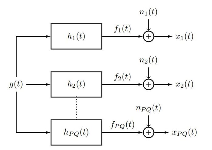
Figure 1: Single input multiple output model is assumed for the video. It is assumed that all the LTI systems (pixels) having different system responses are driven by the same input $g(t)$. Also, every pixel has its own additive noise source.

Under this model, the mathematical problem of interest is: Given $x_{1}(t),x_{2}(t),.....,x_{PQ}(t)$, and that $h_{1}(t),h_{2}(t),......,h_{PQ}(t)$ are unknown, obtain an estimate of $g(t)$, denoted by $\hat{g}(t)$ which is equal to $g(t)$ up to an amplitude scaling factor. That is, estimate $\hat{g}(t)=cg(t)$ where $c$ is an arbitrary constant. This is intractable in general since no information regarding the transfer functions of the LTI systems is available. However, we show that a recovery of $\hat{g}(t)$ is possible if certain assumptions are made about the characteristics of $g(t)$. Specifically, if $g(t)$ is periodic, we show in the subsequent sections that it is possible to recover $\hat{g}(t)$. To start with, we develop the theory for the case of a pure tone ($g(t)$ being a single frequency sinusoid) and further extend it to the case of a general periodic signal.

II-B Solution for a pure-tone case: Lemma - 1

Let $g(t)=Gsin(w_{0}t+\theta)$. From the LTI system theory, the output response of each LTI channel (denoted by $f_{i}(t)$) will be of the following form: $f_{i}(t)=GF_{i}sin(w_{0}t+\phi_{i}+\theta)$ where $F_{i}$ = $|H_{i}(w_{0})|$ and $\phi_{i}=\angle H_{i}(w_{0})$ which are both unique and unknown for each LTI channel. Now, from Eq. 1, $x_{i}(t)=GF_{i}sin(w_{0}t+\phi_{i}+\theta)+n_{i}(t)$. The following lemma demonstrates the existence of an estimator for $g(t)$.

Lemma 1.

If $g(t)$ is a single frequency sinusoid, the ensemble average of LTI output responses taken over a membership set $X^{+}$, defined as

$$X^{+}=\left\{\begin{array}[]{lr}x_{i}(t):|\phi_{i}|\leq\pi/2\\ \forall i\in\{1,...,PQ\}\end{array}\right\}$$

asymptotically converges to a scaled version of the generating signal $g(t)$. Mathematically,

$$\hat{g}(t)=\frac{1}{\overline{X^{+}}}\sum_{i\in X^{+}}x_{i}(t)=cg(t)$$ (2)

Here for any set $A$, operator $\overline{A}$ denotes the cardinality of set $A$.

Proof:

From Eq. 2,

$$\hat{g}(t) = \frac{1}{\overline{X^{+}}}\sum_{i\in X^{+}}x_{i}(t)$$ (3)

$$= \frac{1}{\overline{X^{+}}}\sum_{i\in X^{+}}GF_{i}sin(w_{0}t+\phi_{i}+\theta)+n_{i}(t)$$ (4)

For very large $\overline{X^{+}}$, that is ${\overline{X^{+}}}\to\infty$, the summation in Eq. 4 may be replaced by an expectation operator (over the joint distribution of random variables $F_{i}$, $\phi_{i}$ and $n_{i}$, taken over the set corresponding to $X^{+}$) at every time instant $t$, by the law of large numbers. Thus,

$$\hat{g}(t)=E_{F\phi n}[GF_{i}sin(w_{0}t+\phi_{i}+\theta)+n_{i}(t)]$$ (5)

With the assumption of independence between $\phi$, $F$ and noise and with the linearity of the expectation operator, Eq. 5 may be split as follows, with $E_{F}$, $E_{\phi}$ and $E_{n}$ representing the expectations under the distributions over the random variables $F$, $\phi$ and $n$, respectively over the set $X^{+}.$

$$\hat{g}(t)=GE_{F}[F_{i}]E_{\phi}[sin(wt+\phi_{i}+\theta)]+E_{n}[n_{i}]$$ (6)

By definition, it follows that, over the set corresponding to $X^{+}$, $\phi\in[\frac{-\pi}{2},\frac{\pi}{2}]$ albeit the support of $\phi$ is $[-\pi,\pi]$. Therefore, in Eq. 6,

$$E_{\phi}[sin(wt+\phi_{i}+\theta)] = \frac{1}{\pi}\int_{-\frac{\pi}{2}}^{\frac{\pi}{2}}sin(wt+\phi+\theta)d\phi$$ (7)

$$= \frac{sin(wt+\theta)}{\pi}$$

Thus, with noise process being zero-mean and from Eq. 6 and Eq. 7,

$$\hat{g}(t)=GE_{F}[F_{i}]\frac{sin(wt+\theta)}{\pi}$$

Thus, $\hat{g}(t)\to cGsin(wt+\theta)\qquad\textrm{for}\qquad{\overline{X^{+}}}\to\infty$ where $c=E_{F}[F_{i}]/{\pi}$. ∎

Lemma 1 asserts that the ensemble average of the output responses of a group of LTIs belonging to a set $X^{+}$, converges to the scaled version of the input, when the input is a pure tone. Such an ensemble averaging will also reduce the additive noise in the responses. Although the existence of such a set cannot be guaranteed for every problem, it can be empirically argued that such a set is very likely to exist for the cases considered in the current problem of RP estimation. The rest of this section describes a method for determining the set $X^{+}$ from a given large set of LTI channel responses.

II-C Finding $X^{+}$ - Quadratic approximation

Finding $X^{+}$ through a brute-force method (using its definition) is not feasible because computing phase difference between two signals corrupted with noise is non-trivial. This is because the phase lag introduced by each LTI channel and its associated noise level are unknown. Hence, in this section, we describe an effective method that would not only serve to estimate g(t) by choosing $X^{+}$, but also aids in noise reduction.

It was seen in the previous section that the responses of random LTI channels to a pure tone excitation signal results in a set of randomly scaled and shifted sinusoids (see $x_{i}(t)$), which have two degrees of freedom namely random amplitude scale and phase shift. Intuitively, such a set of random sinusoids can be mapped isomorphically to a two-dimensional space in which the arbitrary amplitude and the phase-lag are better represented. We propose to represent each of the LTI channel responses using a basis set derived out of standard second degree polynomials. Following section lists a set of definitions used to formalize the treatment.

II-C1 Some definitions and notations

Let $x(t)$ and $y(t)$ represent two finite energy signals in Hilbert space ($\mathscr{H_{2}}$) and let $x(t)$ be periodic with $w_{0}$ denoting its dominant frequency - the frequency with the highest magnitude in the Fourier line spectrum of $x(t).$ We define the inner-product between $x(t)$ and $y(t)$ as in Eq. 8 described below.

$$\langle x(t),y(t)\rangle=\frac{w_{0}}{2\pi}\int_{\frac{-\pi}{w_{0}}}^{\frac{\pi}{w_{0}}}x(t)y(t)\,\,dt$$ (8)

The norm of a signal $x(t)$ is defined as $||x(t)||^{2}=\mathbf{\langle}x(t),x(t)\rangle$. Note that the value of inner-products and norms are frequency dependent. We derive a set of basis $\varPsi=\{\psi_{1}(t,w_{0}),\psi_{2}(t,w_{0}),\psi_{3}(t,w_{0})\}$ by orthonormalization of the standard polynomial basis $\Omega=\{1,t,t^{2}\}$ using the Gram-Schmidt procedure. This is to facilitate the easy computation as evident in the subsequent sections. The individual components of $\varPsi$ are given by the following equations.

$$\psi_{1}(t,w_{0}) = \frac{3\sqrt{5}}{2\pi^{2}}w_{0}^{2}t^{2}-\frac{\sqrt{5}}{2}$$ (9)

$$\psi_{2}(t,w_{0}) = \frac{\sqrt{3}}{\pi}w_{0}t$$ (10)

$$\psi_{3}(t,w_{0}) = 1$$ (11)

II-C2 Projection of signals on to the basis $\varPsi$

Let $Q(t)$ as denoted in Eq. 12 represent the span of the basis $\varPsi$ in $\mathcal{\mathtt{\mathscr{R^{3}}}}$.

$$Q(t)\triangleq a\psi_{1}(t,w_{0})+b\psi_{2}(t,w_{0})+c\psi(t,w_{0})$$ (12)

where $a,b$ and $c$ are real numbers. The optimal coefficients $\{a^{*},b^{*},c^{*}\}$ representing the best fit of a signal $s(t)$ in the span of $\varPsi$ are obtained by solving the optimization problem in Eq. 13.

$$\{a^{*},b^{*},c^{*}\}=argmin_{\{a,b,c\}}||Q(t)-s(t)||^{2}$$ (13)

Denoting the error function as $E$, the optimal solution to the problem in Eq. 13 is obtained by simultaneously solving $\partial E/\partial a=0,\,\,\,\partial E/\partial b=0$ and $\partial E/\partial c=0$ which yields the following equations:

$$\mathbb{V}\begin{bmatrix}a^{*}\\ b^{*}\\ c^{*}\end{bmatrix}=\begin{bmatrix}\langle s(t),\psi_{1}(t,w_{0})\rangle\\ \langle s(t),\psi_{2}(t,w_{0})\rangle\\ \langle s(t),\psi_{3}(t,w_{0})\rangle\end{bmatrix}$$ (14)

where $\mathbb{V}_{i,j}=\langle\psi_{i},\psi_{j}\rangle$. Noting that under the defined basis, $\mathbb{V}$ is an identity matrix, from Eq. 14,

$$a^{*} = \langle s(t),\psi_{1}(t,w_{0})\rangle$$

$$b^{*} = \langle s(t),\psi_{2}(t,w_{0})\rangle$$ (15)

$$c^{*} = \langle s(t),\psi_{3}(t,w_{0})\rangle$$

It is to be observed that $c^{*}$ is the mean of the signal $s(t)$ which can be forced to zero if all signals are enforced to be zero-mean. In the rest of the paper, we omit $c^{*}$ since we only consider zero-mean signals. Representation of each of the output responses of the aforementioned random LTI systems ($x_{i}(t)$) using the quadratic approximation may be summarized using the following lemma.

Lemma 2.

Let $s_{i}(t)=sin(w_{0}t+\phi_{i}+\theta)$ and let $\left\{a_{i}^{*},b_{i}^{*}\right\}$ represent the solution for the optimization problem in Eq. 13. Let$\left\{\mathscr{A},\mathcal{\mathscr{B}}\right\}$denote the points spanned by all the solutions for $\phi_{i}\sim\mathscr{\mathbb{U}}\left[-\pi,\pi\right]$, then $\left\{\mathscr{A},\mathcal{\mathscr{B}}\right\}$ lies on the periphery of an ellipse in the solution space. Here $\mathbb{U}$ denotes a uniform distribution.

1. Corollary 1: The major axis of the ellipse is the line corresponding to $\phi=-\theta$.

2. Corollary 2: If $s_{i}(t)=$$\alpha_{i}sin(wt+\phi_{i}+\theta)$ with $\alpha_{i}\leq\alpha_{max}$ the solution space will lead to a filled ellipse with the distance of a point from center of the ellipse being proportional to the corresponding amplitude.

Proof:

It is easy to see that

$$a_{i}^{*} = \langle sin(w_{0}t+\phi_{i}+\theta),\psi_{1}(t,w_{0})\rangle$$ (16)

$$= \frac{3\sqrt{5}}{\pi^{2}}sin(\phi_{i}+\theta)$$

And similarly,

$$b_{i}^{*} = \langle sin(w_{0}t+\phi_{i}+\theta),\psi_{2}(t,w_{0})\rangle$$ (17)

$$= \frac{\sqrt{3}}{\pi}cos(\phi_{i}+\theta)$$

for $\phi_{i}\sim\mathscr{\mathbb{U}}\left[-\pi,\pi\right]$, equations for $a_{i}^{*}$and $b_{i}^{*}$ represent the parametric form for an ellipse in the space of $a$ and $b$ whose major axis corresponds to the line $\phi_{i}+\theta=0$ or $\phi_{i}=-\theta$. Also, for $s_{i}(t)=$$\alpha_{i}sin(wt+\phi_{i}+\theta)$,

$$a_{i}^{*}=\alpha_{i}\frac{3\sqrt{5}}{\pi^{2}}sin(\phi_{i}+\theta)$$ (18)

and

$$b_{i}^{*}=\alpha_{i}\frac{\sqrt{3}}{\pi}cos(\phi_{i}+\theta)$$ (19)

which are concentric ellipses for different $\alpha_{i}$ which are bounded within the ellipse for $\alpha_{i}=\alpha_{max}$. ∎

II-D Extension to a general periodic signal

The discussion so far has only dealt with a pure-tone albeit in practice the signals that are encountered will have multiple harmonics. In this section, the extensions of Lemmas 1 and 2 to the case of general periodic signal will be discussed. Let

$$g(t)=\sum_{k=1}^{\infty}G_{k}sin(w_{k}t+\theta)$$ (20)

be the generating signal of interest. In the rest of the paper, for simplicity of analysis we restrict the Fourier representation of $g(t)$ to $N$ significant harmonics each at $w_{k}$.

II-D1 Estimator for a general periodic signal

From Sections II A and B for this case of $g(t)$,

$$x_{i}(t)=\sum_{k=1}^{N}G_{k}F_{i}(w_{k})sin(w_{k}t+\phi_{i}(w_{k})+\theta)+n_{i}(t)$$ (21)

where $F_{i}(w_{k})=|H_{i}(w_{k})|$ and $\phi_{i}(w_{k})=\angle H_{i}(w_{k})$. With these definitions, Lemma 3 describes the condition for the previously defined estimator, that is, $\hat{g}(t)=\frac{1}{\overline{X^{+}}}\sum_{i\in X^{+}}x_{i}(t)$ to converge to $cg(t)$, in addition to that laid in Lemma 1.

Lemma 3.

$\hat{g}(t)$ converges to $g(t)$ for ${\overline{X^{+}}}\to\infty$ if ${E_{F}[F_{i}(w_{k})]}=constant\,\,\,,\forall k$.

Proof:

By definition,

$$\hat{g}(t)=\sum\limits_{i\in X^{+}}\sum\limits_{k=1}^{N}G_{k}F_{i}(w_{k})sin(w_{k}t+\phi_{i}(w_{k})+\theta)+n_{i}(t)$$

Now, if the phase delay offered by all the channels is assumed to be a constant at all $w_{k}$, $\phi_{i}(w_{k})$ will be independent of $w_{k}$ which can be represented as $\phi_{i}$. As in Lemma 1, for very large $\overline{X^{+}}$, that is $\overline{X^{+}}\to\infty$, the outer summation in the definition of $\hat{g}(t)$ can be replaced by an expectation operator by the law of large numbers. Thus,

$$\hat{g}(t) = E[\sum_{k=1}^{N}G_{k}F_{i}(w_{k})sin(w_{k}t+\phi_{i}+\theta)+n_{i}(t)]$$ (22)

$$= \sum_{k=1}^{N}G_{k}E_{F}[F_{i}(w_{k})]E_{\phi}[sin(w_{k}t+\phi_{i}+\theta)]+E_{n}[n_{i}]$$

$$= \sum_{k=1}^{N}G_{k}E_{F}[F_{i}(w_{k})]\frac{sin(w_{k}t+\theta)}{\pi}$$

Note that in the above expressions as in the case with Lemma 1

$$E_{\phi}[sin(w_{k}t+\phi_{i}+\theta)]=\frac{sin(w_{k}t+\theta)}{\pi}$$ (23)

over set $X^{+}$. From Eq. 22,

$$\hat{g}(t)\to c\sum\limits_{k=1}^{N}G_{k}sin(w_{k}t+\theta)$$

for $\overline{X^{+}}\to\infty$ if ${E_{F}[F_{i}(w_{k})]}=c=constant$. ∎

Lemma 3 along with Lemma 1, asserts that $X^{+}$ should be chosen such that the phase-lags introduced by each of the LTI-channels in the set $X^{+}$ should be within $\pi/2$ radians of $\theta$ and ${E_{F}[F_{i}(w_{k})]}=constant$. In the subsequent section, we show that projection of the signals on the aforementioned quadratic basis aids to select points satisfying both the conditions.

II-D2 Quadratic basis projection for general periodic signal

Let the output response of an $i^{th}$ random LTI system described in Sec. II B, when excited by a periodic signal $g(t)$ described by Eq. 24

$$g(t)=\sum\limits_{k=1}^{N}G_{k}sin(w_{k}t+\theta)$$ (24)

where $w_{k}=kw_{0}$, be represented by $f_{i}(t)$, given by Eq. 25.

$$f_{i}(t)=\sum\limits_{k=1}^{N}F_{i}(w_{k})G_{k}sin(w_{k}t+\phi_{i}+\theta)$$ (25)

Lemma 4.

The ensemble of the quadratic fit coefficients $\{a_{i}^{*},b_{i}^{*}\}$ for $f_{i}(t)=\sum\limits_{k=1}^{N}F_{i}(w_{k})G_{k}sin(w_{k}t+\phi_{i}+\theta)$ with $\phi_{i}\sim\mathscr{\mathbb{U}}[0,2\pi]$, defines a filled parametric elliptical disk in the coefficient space.

Proof:

From Section, II.C, we know that for any signal $f_{i}(t)$, the least-square quadratic fit coefficients $\{a_{i}^{*},b_{i}^{*}\}$ on a basis set $\varPsi$ are given by $a_{i}^{*}=\langle f_{i}(t),\psi_{1}(t,w_{0})\rangle$ and $b_{i}^{*}=\langle f_{i}(t),\psi_{2}(t,w_{0})\rangle$. From Eq. 9 and 10,

$$a_{i}^{*} = \sum_{k=1}^{N}F_{i}(w_{k})G_{k}\langle sin(w_{k}t+\phi_{i}+\theta),\psi_{1}(t,w_{0})\rangle$$ (26)

$$= \sum_{k=1}^{N}F_{i}(w_{k})G_{k}I_{i}^{k}$$ (27)

where $I^{k}_{i}={\langle sin(w_{k}t+\phi_{i}+\theta),\psi_{1}(t,w_{0})\rangle}$, the $k^{th}$ inner product term in Eq. 27. Noting that $w_{k}=kw_{0}$,

$$I_{i}^{k} =\frac{3\sqrt{5}}{\pi^{2}}sin(\phi_{i}+\theta)\frac{(-1)^{k}}{k^{2}}$$ (28)

Following the linearity of the inner products and Eq. 27 and 28,

$$a_{i}^{*} =\frac{3\sqrt{5}}{\pi^{2}}sin(\phi_{i}+\theta)\sum_{k=1}^{N}F_{i}(w_{k})G_{k}\frac{(-1)^{k}}{k^{2}}$$ (29)

Similarly,

$$b_{i}^{*} =\frac{\sqrt{3}}{\pi}cos(\phi_{i}+\theta)\sum_{k=1}^{N}F_{i}(w_{k})G_{k}\frac{(-1)^{k+1}}{k}$$ (30)

Since the summation terms in Eq. 29 and 30 converge to a finite number, $\{a_{i}^{*},b_{i}^{*}\}$ define a parametric ellipse for $\phi_{i}\sim\mathscr{\mathbb{U}}[-\pi,\pi]$. Also, depending upon the values of the product terms $F_{i}(w_{k})G_{k}$, they converge to a different number, leading to a filled ellipse. ∎

The following are some of the major implications of Lemma 4 which are to be noted.

1. Every point on the filled ellipse corresponds to an LTI channel with a certain magnitude and phase response.

2. The major axis corresponds to the that LTI channel with a phase response $\phi_{i}=-\theta$ . LTI channels with all other phase shifts ($\phi_{i}$) are symmetrically and uniformly distributed around the major axis.

3. A set of LTI channels with the same magnitude response but different phase response correspond to points lying on an elliptical ring inside the disk. This is evident from Eq. 29 and 30, where, for the LTI channels with same magnitude response, $F_{i}(w_{k})$ is independent of $i$. Further, since $G_{k}$ is fixed, $\{a_{i}^{*},b_{i}^{*}\}$ for such a set defines an ellipse with a fixed length major and minor axis.

4. If the generating signal is assumed to be of a low-pass nature, that is, $|G_{k}|>|G_{k+1}|$, the points closer to the periphery of the disk, correspond to the LTI channels that emphasize fundamental frequency the most, over the harmonics. This is because, in this case, the summation terms in Eq. 29 and 30 are monotonically decreasing series with alternating sign.

5. The points that are farther away from the periphery of the disk, correspond to the LTI channels that attenuate the fundamental frequency while emphasizing the higher harmonics.

Fig. 2 demonstrates Lemma 4 and some of its implications.

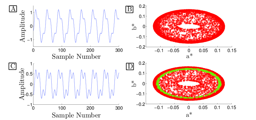
Figure 2: Demonstration of Lemma 4 and its implications : (A) and (B) respectively depict the generating signal ($g(t)=sin(50\pi t)+\frac{1}{3}sin(150\pi t)$) and the elliptical disk generated from quadratic fit coefficients corresponding to the outputs of several random LTI channels. (C) depicts the output of a random LTI channel with a given magnitude response, when excited by $g(t).$ (D) is the disk in (B), with the elliptical ring corresponding to set of LTI channels with the magnitude response used to obtain the signal (C), marked by green dots.

II-E Impact of noise on the coefficients

The model proposed in Sec. II A, involves an additive noise component associated with each pixel (LTI channel) that has not been considered in all the analysis so far. In this section, the impact of additive noise on the coefficients obtained from quadratic polynomial fitting is discussed.

For a periodic excitation signal $g(t)=\sum\limits_{k=1}^{N}G_{k}sin(w_{k}t+\theta)$, from Sec. II A, we have the response of each individual LTI system,

$$x_{i}(t)=f_{i}(t)+n_{i}(t)$$ (31)

with

$$f_{i}(t)=\sum\limits_{k=1}^{N}F_{i}(w_{k})G_{k}sin(w_{k}t+\phi_{i}+\theta)$$ (32)

From Sec. II.C.2, we know that the quadratic coefficients for the signal $x_{i}(t)$ are given by $\hat{a}_{i}=\langle x_{i}(t),\psi_{1}(t,w_{0})\rangle$, $\hat{b}_{i}=\langle x_{i}(t),\psi_{2}(t,w_{0})\rangle$ and because we are working with zero-mean signals, $c_{i}^{*}=0$. Since the inner products are linear,

$$\hat{a}_{i} = \langle f_{i}(t),\psi_{1}(t,w_{0})\rangle+\langle n_{i}(t),\psi_{1}(t,w_{0})\rangle$$ (33)

$$\hat{b}_{i} = \langle f_{i}(t),\psi_{2}(t,w_{0})\rangle+\langle n_{i}(t),\psi_{2}(t,w_{0})\rangle$$ (34)

Let $\langle f_{i}(t),\psi_{1}(t,w_{0})\rangle=a_{i}^{*}$ and $\langle f_{i}(t),\psi_{2}(t,w_{0})\rangle=b_{i}^{*}$ represent the solution for the no-noise case. Given the aforementioned definitions, the objective is to relate $\{\hat{a}_{i}$,$\hat{b}_{i}\}$ to $\{a_{i}^{*},b_{i}^{*}\}$. We have,

$$\hat{a}_{i} = a_{i}^{*}+\langle n_{i}(t),\psi_{1}(t,w_{0})\rangle$$ (35)

$$\hat{b}_{i} = b_{i}^{*}+\langle n_{i}(t),\psi_{2}(t,w_{0})\rangle$$ (36)

From Cauchy-Shwartz inequality,

$$-\sigma \leq \langle n_{i}(t),\psi_{1}(t,w_{0})\rangle\leq\sigma$$ (37)

$$-\sigma \leq \langle n_{i}(t),\psi_{2}(t,w_{0})\rangle\leq\sigma$$ (38)

where $||n_{i}(t)||^{2}=\sigma^{2}$ and $||\psi_{i}||^{2}=1$, by definition. Thus from Eq. 35, 36, 37 and 38,

$$a_{i}^{*}-\sigma\leq \hat{a}_{i} \leq a_{i}^{*}+\sigma$$ (39)

$$b_{i}^{*}-\sigma\leq \hat{b}_{i} \leq b_{i}^{*}+\sigma$$ (40)

From Eq. 39 and 40, it can be inferred that with the addition of noise, $\{a_{i}^{*},b_{i}^{*}\}$ gets perturbed within a cloud bounded by $|\sigma|$.Since there is no natural comparative bound of the relative magnitudes of noise and coefficients, nothing can be inferred regarding the relation between the position of a given point in the coefficient space and the quality of the signal. However, useful insights can be obtained if all the signals are normalized (forced to be unit norm) prior to quadratic fitting. Let the signal-to-noise-ratio (SNR) corresponding to $i^{th}$ LTI channel denoted by $\rho_{i}$, be defined as $\rho_{i}\triangleq||f_{i}(t)||/||n_{i}(t)||.$ With these notations, the following Lemma relates $\{\hat{a}_{i},\hat{b}_{i}\}$, $\{a_{i}^{*},b_{i}^{*}\}$ and $\rho_{i}.$

Lemma 5.

When random noise $n_{i}(t)$ is added to $f_{i}(t)$ to yield $x_{i}(t)$, the quadratic coefficients $\{a_{i}^{*},b_{i}^{*}\}$ corresponding to normalized $f_{i}(t)$ get scaled by a factor less than unity and perturbed within a cloud whose area is inversely proportional to $\rho_{i}^{2}$ to yield the quadratic coefficients corresponding to the noisy signal.

Proof:

Let $x_{i}(t)$ be forced to have unit norm before quadratic approximation to yield $\tilde{x}_{i}(t)$ $=x_{i}(t)/||x_{i}(t)||$. By definition,

$$||x_{i}(t)||^{2} = ||f_{i}(t)+n_{i}(t)||^{2}$$

$$= ||f_{i}(t)||^{2}+||n_{i}(t)||^{2}$$

$$= \sigma^{2}(\rho_{i}^{2}+1)$$

because $\langle f_{i}(t),n_{i}(t)\rangle=0$. Note that

$$a_{i}^{*} = \langle f_{i}(t)/||f_{i}(t)||,\psi_{1}(t,w_{0})\rangle$$ (42)

$$\Rightarrow |f_{i}(t)||a_{i}^{*}=\langle f_{i}(t),\psi_{1}(t,w_{0})\rangle$$ (43)

$$b_{i}^{*} = \langle f_{i}(t)/||f_{i}(t)||,\psi_{2}(t,w_{0})\rangle$$ (44)

$$\Rightarrow ||f_{i}(t)||b_{i}^{*}=\langle f_{i}(t),\psi_{2}(t,w_{0})\rangle$$ (45)

Let $\{\hat{a}_{i},\hat{b}_{i}\}$ denote the quadratic coefficients for $\tilde{x}_{i}(t)$. From Lemma 2, we have

$$\hat{a}_{i} = \frac{||f_{i}(t)||a_{i}^{*}}{||x_{i}(t)||}+\frac{\langle n_{i}(t),\psi_{1}(t,w_{0})\rangle}{||x_{i}(t)||}$$ (46)

$$\hat{b}_{i} = \frac{||f_{i}(t)||b_{i}^{*}}{||x_{i}(t)||}+\frac{\langle n_{i}(t),\psi_{2}(t,w_{0})\rangle}{||x_{i}(t)||}$$ (47)

From Eq. 46, 47, 37 and 38,

$$\frac{||f_{i}(t)||a_{i}^{*}}{||x_{i}(t)||}-\frac{\sigma}{||x_{i}(t)||}\leq \hat{a}_{i}\leq\frac{||f_{i}(t)||a_{i}^{*}}{||x_{i}(t)||}+\frac{\sigma}{||x_{i}(t)||}$$ (48)

$$\frac{||f_{i}(t)||b_{i}^{*}}{||x_{i}(t)||}-\frac{\sigma}{||x_{i}(t)||}\leq \hat{b}_{i}\leq\frac{||f_{i}(t)||b_{i}^{*}}{||x_{i}(t)||}+\frac{\sigma}{||x_{i}(t)||}$$ (49)

Using the definition of $||x_{i}(t)||^{2}$ in Eq. 48 and 49,

$$\frac{\rho_{i}a_{i}^{*}}{\sqrt{\rho_{i}^{2}+1}}-\frac{1}{\sqrt{\rho_{i}^{2}+1}}\leq \hat{a}_{i}\leq\frac{\rho_{i}a_{i}^{*}}{\sqrt{\rho_{i}^{2}+1}}+\frac{1}{\sqrt{\rho_{i}^{2}+1}}$$ (50)

$$\frac{\rho_{i}b_{i}^{*}}{\sqrt{\rho_{i}^{2}+1}}-\frac{1}{\sqrt{\rho_{i}^{2}+1}}\leq \hat{b}_{i}\leq\frac{\rho_{i}b_{i}^{*}}{\sqrt{\rho_{i}^{2}+1}}-\frac{1}{\sqrt{\rho_{i}^{2}+1}}$$ (51)

From Eq. 50 and 51, since ${\rho_{i}}/{\sqrt{{\rho_{i}}^{2}+1}}\leq 1$ the factor scaling $a_{i}^{*}$ is less than unity and the area of the cloud of perturbation is ${({{{\rho_{i}}^{2}+1}})}^{-1}$. ∎

One of the primary implications of Lemma 5 is that for a given amount of noise power $\sigma$, the signals having a higher $||f_{i}(t)||$ will have a higher SNR $\rho_{i}$. From Lemma 4, it is known that, for a low-pass signal, the LTI channels that emphasize the fundamental frequency over the others will have a higher $||f_{i}(t)||$ and hence a higher SNR. This implies that such LTI channels (mapping to points closer to the periphery of the elliptical disk defined in Lemma 4) are likely to be perturbed the least and have a smaller cloud of perturbation.This fact is illustrated in Fig. 3 with an example.

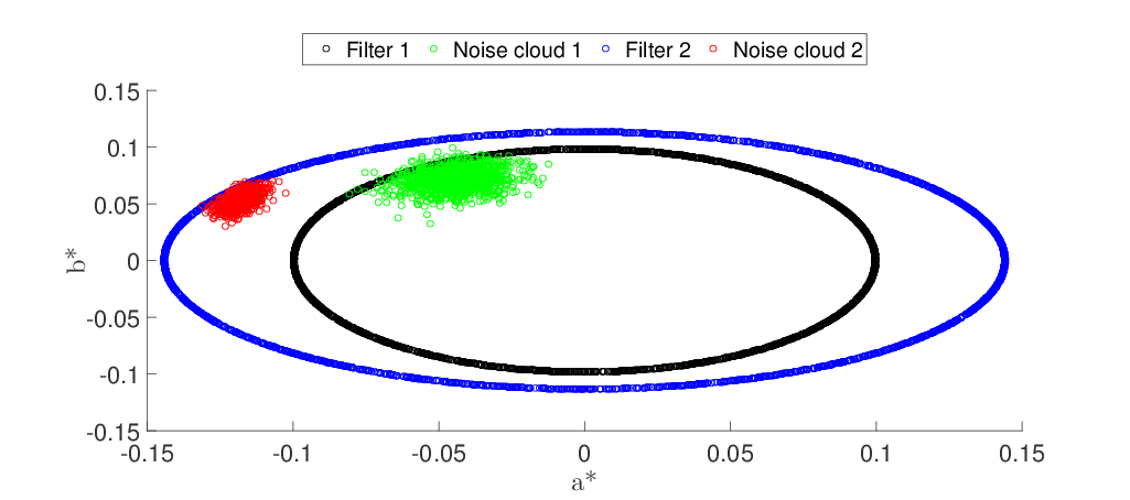
Figure 3: Illustration of Lemma 5 - Ellipses in blue and black, respectively, represent the quadratic coefficient space for the output of two sets of LTI channels with magnitude response $[F_{1}(40\pi),F_{1}(80\pi)]=\{0.8,0.1\}$ and$[F_{2}(40\pi),F_{2}(80\pi)]=\{0.2,0.8\}$ and phase shifts defined by$\phi_{i}\sim\mathscr{\mathbb{U}}[-\pi,\pi]$ driven by a same generating signal $g(t)=sin(40\pi t)+0.5sin(80\pi t)$. Thousand samples of Gaussian noise process with $\sigma=0.5$ are generated and added to the output of one LTI channel with a fixed phase taken from each set. The quadratic fits for the noisy signals are shown using red and green dots. It can be seen that for the same amount of noise power, the area of cloud of perturbation is lower for the LTI channel that lies exterior which corresponds to the LTI channel emphasizing the fundamental frequency.

II-F Selection of an optimum membership set

II-F1 Criteria for optimality

All the discussions so far are aimed towards selecting a membership set $X^{+}$over which an ensemble average has to be computed to get an estimate of the generating signal. In this section, we consolidate all the criteria that are developed in previous sections to select $X^{+}$ and map them to geometrical locations on the elliptical disks obtained through quadratic fitting. The theory developed so far lays the following criteria for optimality of the selected $X^{+}$.

1. There need to be enough channels in $X^{+}$ so that expectations in all the Lemmas are well approximated by summations.

2. Lemma 3 demands that for accurate estimation of $g(t)$, $E_{F}(F(w_{k}))=constant.$ Note also that there can be multiple LTI channels having identical magnitude responses. This implies that, to satisfy condition laid in Lemma 3, every type of LTI channel magnitude response should receive equal weightage in $X^{+}$.

3. The phase-lags introduced by each channel in $X^{+}$ must be within $\pi/2$ radians of the phase of the generating signal $\theta$.

4. With the addition of noise the channels selected should be such that the phase distortion caused by the noise should not violate condition 3.

Any half elliptical arc about the major axis of the disk will ensure that condition 3 is satisfied. From Lemma 4 the points on the periphery of the ellipse should be complemented by points on the interior to satisfy condition 2. An ideal choice which will ensure that both conditions 1 and 2 are met would be to take the entire half ellipse. This is because $F(w_{k})$ is modeled as an IID random variable whose expectation would converge to a fixed number and LTI channels with same magnitude response are represented along the radial arcs of the disk for $\phi_{i}\sim\mathbb{U}[-\pi,\pi$]. However, with noise, inclusion of points that are interior on the disk will distort the morphology of the estimated generating signal by violating condition 3. Hence, we propose to select the channels by aggregating along half elliptical arcs starting from the periphery. However, since the points close to the periphery emphasize the fundamental frequency and the interior points emphasize the higher harmonics, as we move inwards, there is a trade-off between getting better estimates of the higher harmonics and reducing the impact of noise on the obtained estimate .

II-F2 Choice of $X^{+}$

The optimal choice of $X^{+}$ should adhere to all the criteria listed above and also to handle the aforementioned trade-off. We propose to select $X^{+}$ as a set difference between two sets of points on the feature elliptical disk.

Let $\{a_{i},b_{i}\}$ represent a point on the ellipse, $i\in\{1,...,PQ\}$. Let $A=max(a_{i})$ and $B=max(b_{i})$. Define two sets $D_{O}$ and $D_{I}$ that would correspond to certain regions within the disk.

$$D_{O}={}\{ a_{i},b_{i}:a_{i}\leq Asin(\phi_{i}+\theta),$$ (52)

$$b_{i}\leq Bcos(\phi_{i}+\theta),$$

$$\forall i:|\phi_{i}|\leq\frac{\pi}{2}\}$$

$$D_{I}={}\{ a_{i},b_{i}:a_{i}\leq r_{e}Asin(\phi_{i}+\theta),$$ (53)

$$b_{i}\leq r_{e}Bcos(\phi_{i}+\theta),$$

$$\forall i:|\phi_{i}|\leq\frac{\pi}{2}\}$$

where $0<r_{e}\leq 1$ denotes the radius of exclusion.

$$X^{+}=D_{O}\backslash D_{I}$$ (54)

Notice that $D_{O}$ is set of all points within half the disk along the major axis pointing towards $\phi_{i}=\theta$, which can also be viewed as set of all points within a half ellipse whose major axis is $A$. $D_{I}$ is a subset of $D_{O}$ consisting of points within an ellipse with the length of major and minor axes as $r_{e}A$ and $r_{e}B$, respectively, where $r_{e}\leq 1$ is a parameter of the method termed the radius of exclusion. A goodness-of-estimation (GoE) measure is defined (in the subsequent section) which would determine the ‘best’ choice of this parameter for the selection of $X^{+}$. Figure 4 illustrates the aforementioned procedure for selection of $X^{+}$ using an example elliptical disk in the feature space.

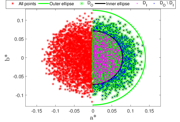
Figure 4: Illustration of procedure to select $X^{+}$. Every point on the elliptical disk (red crossed points) correspond to one LTI channel. Green solid line is the outermost half ellipse which defines the set $D_{O}$ (all the points on one half of the disk within the outermost ellipse, marked by green star points). A choice of radius of exclusion $r_{e}$, defines an inner ellipse (marked by black solid line) which specifies the set $D_{I}$ (the points on one half of the disk within the inner ellipse, marked by pink crossed points). Once the sets $D_{O}$ and $D_{I}$ are selected, $X^{+}$ are taken as the points corresponding to the set difference between $D_{O}$ and $D_{I}$ (marked by blue crossed points). Note that the length of the axes of the inner ellipse depends upon the value of radius of exclusion $r_{e}$.

While an arbitrary value of $r_{e}$ is used in Fig. 4 for an illustration purpose, Fig. 5 illustrates the trade-off between inclusion of more LTI channels (and thus getting a better estimate of higher harmonics) in $X^{+}$ and reducing the impact of noise on the estimate using different values of $r_{e}$ with the corresponding time-domain signals. It is noteworthy that increase in $r_{e}$ (and thus increasing $\overline{D_{I}}$ ) characterizes increase in noise where as it estimates higher harmonics better and vice-versa.

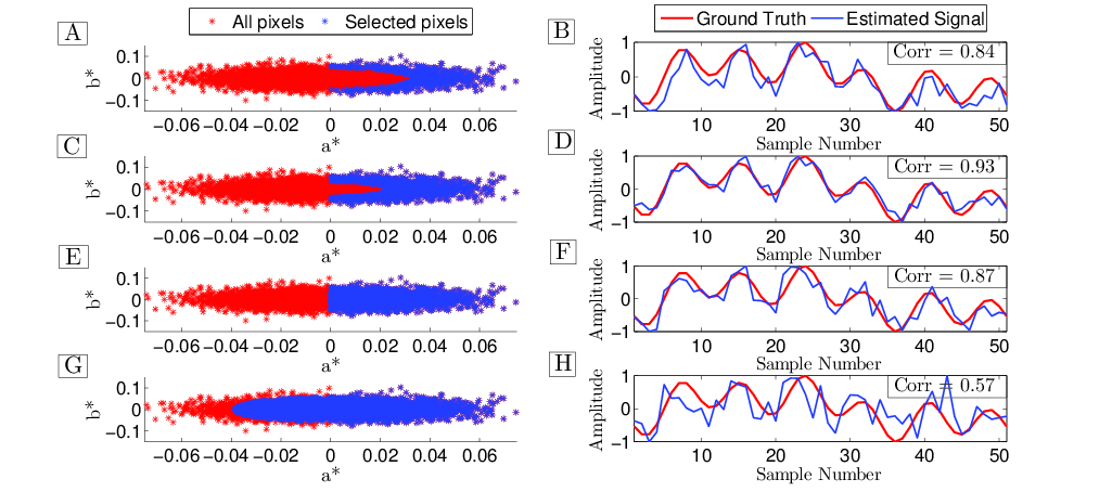
Figure 5: Illustration of the trade-off between inclusion of more LTI channels (and thus getting a better estimate of higher harmonics) in $X^{+}$ and reducing the impact of noise on the estimate: A generating periodic signal with three harmonics is passed through random LTI systems with additive white Gaussian noise as discussed in Sec. II A. (A), (C), (E) and (G) represent the ellipses corresponding to the quadratic fits of the responses of all the random LTI systems to the generating signal, with the LTI channels selected (different set in different cases) to be in $X^{+}$ marked in blue. (B), (D), (F) and (H) show one period of the corresponding estimated signals (blue line) along with the generating signal (red line). It can be seen that the estimate corresponding to the entire half ellipse (E and F) and one having points close to periphery (A and B) do not agree as much as the one with an optimized parameter (C and D). In other words, increase in $r_{e}$ (and thus increasing $\overline{D_{I}}$ ) characterizes an increase in the amount of noise in the estimate. Also, selecting a set of points spanning more than one half of the disk (G and H, violating the definition of $X^{+}$) greatly distorts the signal as mentioned in points 3 and 4 of section II. F. These facts are also corroborated with the value of the normalized correlation coefficients between the estimates and the ground truth as shown in the corresponding figures.

II-G Details of implementation for RP estimation

Implementing the algorithm described in the previous sections for the current problem of respiration pattern estimation involves computation of certain parameters outside of the theoretical description, which will be detailed in this section. Note that for a given video, individual time series (refer to as pixel time series, PTS) corresponding to pixel intensity values of each spatial location for a given duration forms the LTI responses. Also, RP is the generating signal which we seek to estimate.

II-G1 Estimation of basis frequency and measurement residual phase

The quadratic-basis ($\psi$) defined in Sec. II.C.1 is a function of basis-frequency ($w_{0}$). This implies that finding the best-fit coefficients to each PTS requires the a-priori knowledge of $w_{0}$. Although this requirement seems to demand a crucial parameter a priori, it will be shown in the subsequent sections that the inaccuracy in the initial choice of $w_{0}$ does not affect the estimate of the RP. Further, the exact state of the breathing of the subject at the start of the video capture is unknown. This results in a residual phase-lag between the estimated signal and the generating signal which is to be compensated for. We compute a ‘proxy signal’ that would simultaneously estimate $w_{0}$ and compensate for the residual phase. Proxy signal is a time-series whose value at a given time is obtained by taking the element-wise dot product of intensities of all the pixels in the video frame corresponding to that time, with respect to the intensities of the pixels in the very first video frame. Mathematically, if $x(t)$ is the column vector obtained by stacking all the intensity values in frame at time $t$, then the proxy signal $p(t)$ is defined as $p(t)=(\mathbf{x}(1)\cdot\mathbf{x}(t))/(|\mathbf{x}(1)||\mathbf{x}(t)||)$. $p(t)$ being the cosine of angle between two vectors, defines the state of breathing in every frame with respect to the very first frame. Also, it will be periodic and its fundamental frequency is used as the basis frequency $w_{0}$. The residual phase correction is made by projecting one period of the proxy signal on to the data elliptical disk. Further the major axis of the data elliptical disk is reoriented along the direction of the projected point corresponding to the proxy signal.

II-G2 Goodness-of-estimation (GoE) measure for parameter selection

In section II.F, to handle the trade-off between estimating the higher harmonics better and reducing the impact of noise, a GoE measure is described to select the parameter deciding the part of the disk to be included in $X^{+}$. Since the generating signal to be estimated is periodic a measure that quantifies the closeness of a signal to this behaviour will serve as a GoE measure. It is known that the Fourier magnitude spectrum of a periodic signal is sparse and $l_{0}$ norm (number of non-zero elements in a set) of the magnitude spectrum of periodic signals should be lower than that for non-periodic signals. Hence, for aggregation of points to be chosen in $X^{+}$, we start from the periphery and choose the parameter (radius of exclusion, See II.F.) that would result in the least $l_{0}$ norm.

III Experiments and results

The theory and the method proposed in Sec.II is validated using simulated periodic signals and real-life breathing video data. The simulated data serves the purpose of directly verifying the theoretical claims by having a control over all the variables involved whereas the real-life data is to demonstrate the usability of the method in real-life scenarios.

III-A Simulated Data

This data comprises of seven different generating signals of the form $g(t)=\sum_{k=1}^{N}G_{k}sin(w_{k}t+\theta)$ as described in Table I.

TABLE I: Properties of the signals used to to simulate different cases.

Type of the signal $\left(g(t)\right)$	$G_{k}$	$f_{k}(deci\,\,Hz)$
Single frequency	${1}$	${50}$
Two frequencies	${1,\frac{1}{3}}$	${25,75}$
Three frequencies	${1,\frac{1}{3},\frac{1}{2}}$	${20,60,120}$
Four frequencies	${1,\frac{1}{6},\frac{1}{8},\frac{1}{12}}$	${25,50,100,125}$
Sawtooth wave ($N=10$)	$\frac{1}{k}$	$20*k$
Square wave ($N=10$)	$\frac{1}{2k-1}$	$20*(2k-1)$
Triangle wave ($N=10$)	$\frac{(-1)^{k-1}}{(2k-1)^{2}}$	$20*(2k-1)$

Each $g(t)$ is passed through a set (5000 samples, $i$) of random LTI systems connected in parallel to obtain $f_{i}(t)$ (Sec. II.E) with $F_{i}(w_{k})=\mathbb{U}\sim[0,1]$ and $\phi_{i}=\mathbb{U}\sim[-\pi,\pi]$. These responses, $f_{i}(t)$, are added with a noise process $n(t)\sim\mathbb{N}(0,\sigma^{2})$ to yield $x_{i}(t)$. A part of each $x_{i}(t)$ of length corresponding to $w_{0}$ is projected on to the quadratic basis $(\psi$) described in Lemma 4 to obtain the elliptical disks of coefficients.

III-A1 Experiments and validation metrics

We report three experiments as follows - (1) different amounts of noise are added to each $g(t)$ that is estimated using the method described and the normalized cross-correlation between $g(t)$ and the estimated signals are studied, (2) The extent of validity of $l_{0}$norm as the GoE measure is studied against the normalized cross-correlation measured between $g(t)$ and the estimated signals and (3) sensitivity of the method to the choice of the basis frequency ($w_{0}$) is studied by comparing the correlation and the fundamental frequency of the estimated signals (with an improper choice of $w_{0}$) with $g(t)$.

III-A2 Results and discussion

Fig. 6 depicts the cross-correlation between the estimated signals and different $g(t)$ with SNR ranging between -15 to 25 dB.

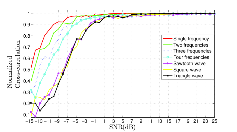
Figure 6: Correlation between the estimated signals and different $g(t)$ with SNR ranging between -15 to 25 dB.

The threshold for radius of exclusion was determined by the $l_{0}$ norm GoE. It is seen that for all the signals, as SNR increases the cross-correlation generally increases and saturates around 1 dB. However, at SNRs lower than -2 dB, a signal with lower number of harmonics achieves a certain cross-correlation before a signal that has higher number of harmonics. It is seen that for all signals the cross-correlation reaches 0.9 around -2 dB implying that this method can recover the signal to a fairly good extent even when noise power is more than that of the signal.

In the next experiment, we fix the SNR at 0 dB and study the properties of the estimated signal by varying the choice of basis-frequency ($w_{e}$) between $0.05w_{0}$ and $2w_{0}$ where $w_{0}$ is the actual fundamental frequency of a given $g(t)$. Fig. 7 (A) depicts the normalized-cross correlation between the estimated signal and $g(t)$ as a function of $\frac{(w_{0}-w_{e})}{w_{0}}$. It is seen that good estimates are obtained only around $w_{e}=w_{0}$ and estimates degrade on either sides. This implies that the method is very sensitive to the choice of $w_{0}$. However, the method can be easily tweaked to circumvent this problem as evident from the following discussion: Fig. 7 (B) depicts the fundamental frequency of the estimated signals as a function of the same $\frac{(w_{0}-w_{e})}{w_{0}}$ as in Fig. 6 (A). It can be seen that the fundamental frequency of all the estimated signals (taken to be the frequency at which the magnitude Fourier spectrum peaks) are exactly the same as that of the corresponding $g(t)$ (as inferred from Table I). This implies that the peak of the magnitude spectrum of the estimated signals is totally insensitive to the choice of basis-frequency and the lower cross-correlation is due to the aggregation of wrong phase lags $(\phi_{i}$) of the LTI channels that are selected in $X^{+}$. This is also supported from the theory because to get a good estimate of the magnitude response it is enough to satisfy criteria 1 and 2 listed in section II.F despite violating criteria 3 and 4. A wrong choice of $w_{0}$ still leads to an elliptical disk but with an improper orientation of $\phi_{i}$ with respect to the actual phase of $g(t)$, $\theta$. In this case the proposed method still picks up the points required for an accurate estimation of the magnitude response albeit distorting the shape of the estimated signal due to the selection of LTI channels with improper phase lags. This suggests that a simple way to circumvent the sensitivity of the method to the choice of $w_{0}$ is to adopt a two-step procedure where the initial step is to derive the actual $w_{0}$ (with any initial choice of $w_{0}$) and in the next step is to use the proper $w_{0}$ to estimate the morphology of $g(t)$.

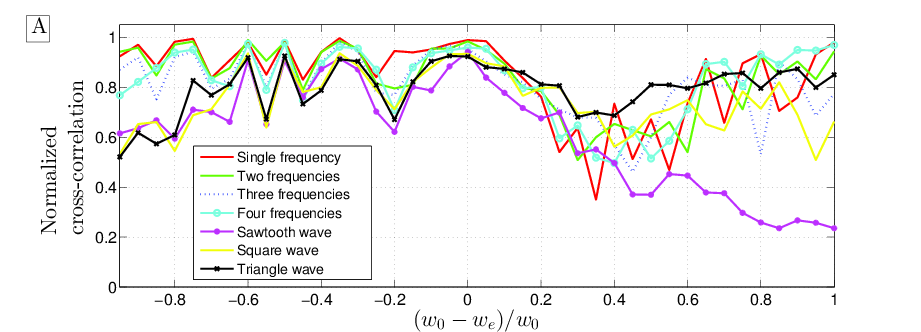
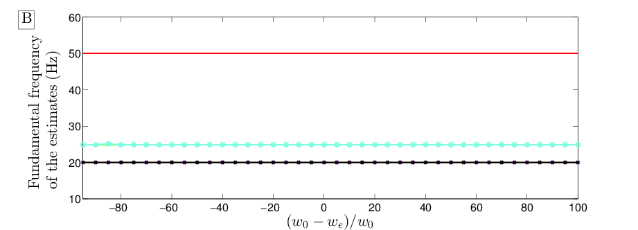
Figure 7: Analysis of sensitivity of the method to the choice of basis frequency. (A): Normalized cross-correlation between the estimated signal and $g(t)$ (B) Fundamental frequency of the estimated signal. Both (A) and (B) are plotted as a function of of $\frac{(w_{0}-w_{e})}{w_{0}}$.

In the proposed method, the optimal choice of the threshold used for selecting the radius of exclusion (discussed in Sec. II.F) is decided based on the GoE metric. In the last experiment, we validate the proposed metric ($l_{0}$ norm of the magnitude spectrum of the estimated signal) by comparing it against the cross-correlation measure. Fig. 8 depicts the values of inverse of $l_{0}$ norm (GoE) of the estimated signals and cross-correlation between the estimated signal and $g(t)$ for three signals: sawtooth, square and triangle wave at $-5$dB SNR as a function of threshold for radius of exclusion. It is to be noted that the value of threshold corresponding to unity represents the selection of all points in one half of the ellipse.

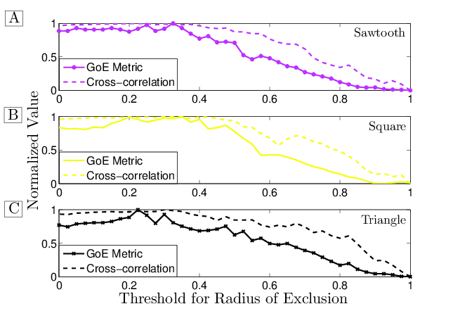
Figure 8: Validation of $l_{0}$ norm as the GoE metric for the selection of optimal choice of the threshold used for selecting the radius of exclusion. Values of inverse of $l_{0}$norm (GoE) of the estimated signals and correlation between the estimated signal and $g(t)$ for three signals - Sawtooth wave (A) and Square wave (B) and Triangle wave (C) at $-5$dB SNR as a function of threshold for radius of exclusion.

The proposed method selects that threshold corresponding to the highest GoE which estimates a signal with a very high correlation with $g(t)$ as seen from Fig.8. This indicates that the defined measure for GoE can be used as a proxy to determine the threshold in the practical cases where the correlation measure cannot be computed due to the unavailability of $g(t)$.

III-B Real-life Dataset

The real-life dataset comprises respiration videos acquired from 31 healthy human subjects (for which institutional approval and subject-consent were obtained) (10 female and 21 male) between ages of 21 - 37 (mean: 28). Six controlled breathing experiments (Fig. 9) (I) normal breathing, (II) deep breathing, (III) fast breathing, (IV) normal-deep-normal breathing (sudden change in breathing volume), (V) normal-fast-normal breathing (sudden change in breathing frequency), (VI) episodes of breath hold, ranging between 13 - 150 (mean: 45) seconds were performed by each subject. The subjects wore a wide variety of clothing with different textures or no upper body clothing (two subjects). Videos were simultaneously recorded from two cameras with resolution of 640X480 pixels at a speed of 30 frames per second, one from the ventral view (VGA) and other from lateral view (2MP) of the subject under normal indoor illumination, each placed at a distance of 3 ft from the subject. The subjects were asked to sit and breath in patterns described above resulting in a total of  2.5 hours of recordings with approximately 2000 respiratory cycles for each side. For validation, an impedance pneumograph (IP) device [6] was connected through electrodes on the chest of the subject, which estimates the RP and RR by quantifying the changes in electrical conductivity of the chest due to respiratory air-flow. This device is routinely used in patient monitors and other applications in which it is considered a medical gold standard [37].

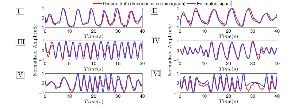
Figure 9: Depiction of six different validation experiments performed : Red curve corresponds to normalized amplitudes of the impedance pneumogram device attached to the subject and blue curves are the estimated signal.

III-B1 Experiments and validation metrics

Given a subject video, the proposed algorithm is applied to estimate the RP and RR retrospectively. A typical frame (as shown in Fig. 10 ) also consists of regions like background wall, that contain pixels that are unaffected by respiration. An image gradient operation is applied over a large rectangular window on two arbitrarily selected frames at the beginning of the video that are spaced apart by the minimum possible RR. Subsequent frames are pruned to contain only those pixels with very high values of the gradient. This selects a smaller region of the frame typically comprising the chest-abdomen region of the subject. Note this operation is done only once on a pair of frames at the beginning of the video. This is to reduce the unnecessary processing of static pixels even though the proposed algorithm does not demand the same. The initial estimate of basis-frequency and the residual measurement phase are obtained using the proxy signal. Quadratic coefficients are obtained for every pixel time series to form the elliptical disk from which the optimum membership set $X^{+}$ and thus the RP are estimated. Once $X^{+}$ is assembled by tagging PTS (which only involves computation of inner products), the algorithm can be executed in real-time since the estimator only computes a pixel average over $X^{+}$. Once the RP is obtained, RR is estimated from the peak in the Fourier magnitude spectrum of the RP taken over a window (typically between 10 and 15 seconds).

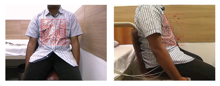
Figure 10: Depcition of an actual data scene with the selected memebership set $X^{+}$ marked in red.

The goal of this study is to estimate the morphology of the respiration airflow signal (RP) and not the actual airflow. Further, the IP device also does not directly provide the volumetric information albeit it has been shown to provide the actual airflow information with proper calibration [6]. Thus we use the Pearson correlation coefficient [38] between the normalized signal obtained from the IP representing the ground truth, GT, and the normalized estimated RP as a measure quantifying the closeness of two signals. This measure lying between -1 and 1 quantifies the closeness of two temporal signals with unity referring to the maximum agreement. RR measurements are validated through the linear regression between GT and the estimated RR values. Further since RR is a frequency measurement that can be exactly obtained from both the signals, the exact agreement is quantified using the Bland-Altman plots [39].

III-B2 Results and discussion

Figure 11 depicts the correlation and agreement of the estimated signals with $g(t)$: (A) and (C) show the degree of linear relationship between RR measurements using webcam and IP device. For the ventral video acquisition, in Fig. 11 (A), it is observed that the correlation coefficient ($r$ ) is 0.94 with $p<0.001$, which shows a strong positive correlation between the measurements. Also, Bland-Altman plots in Fig. 11(B) shows that the RR measurement through webcam has an acceptable average agreement (very low bias of 0.88) with the ground truth with $91\%$ of the measurements within 3BPM of the ground truth. The median of deviation between the estimated values and the GT values is zero and the measurements that are outside of the confidence interval (CI, defined as $\pm$3 BPM of the ground truth values) are often higher than the actual RR. These are the cases where there are high-frequency repetitive and densely patterned textures. For the case of lateral video acquisition, in Fig. 11 (C) and (D), a correlation coefficient ($r$ ) of 0.85 is observed with $p<0.001$ and $87\%$ of the measurements lie within 3 BPM of the ground truth. These numbers are lesser than those for the frontal view because the lateral view typically has much fewer members in $X^{+}$.

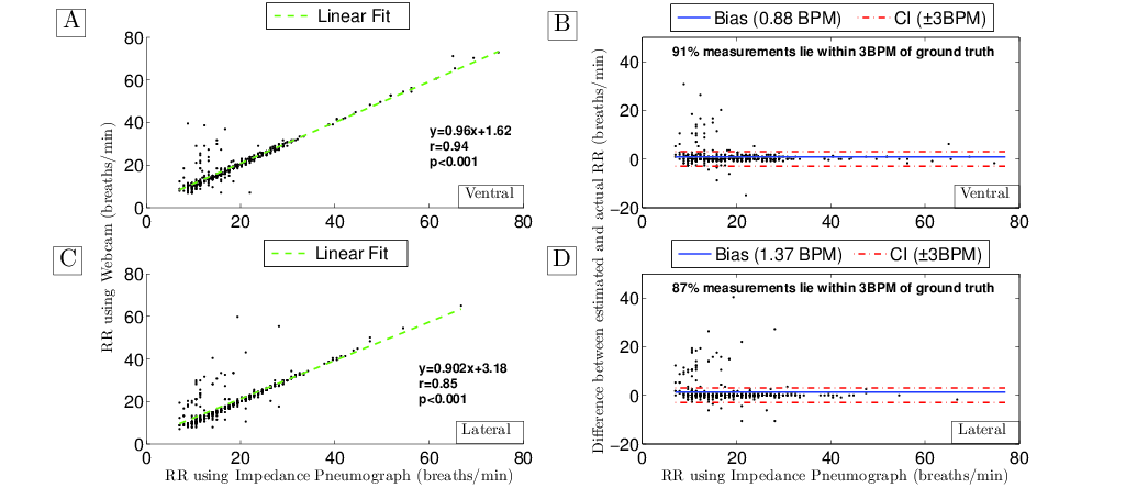
Figure 11: Correlation and agreement of the estimated signals with $g(t)$: (A) and (C) show the degree of linear relationship between RR measurements using webcam and IP device. (B) and (D) are the Bland-Altman plots showing the difference in the RR values with a confidence interval of $\pm 3$ BPM (CI) obtained from the two methods against the ground truth. For the ventral video acquisition, in (A) we observe that the Pearson correlation coefficient ($r$ ) is 0.94 with $p<0.001$, which shows a strong positive correlation between the measurements.

Figure 12 depicts the histograms of the signal correlation measure between the estimated RP and GT for different cases. It is seen that the mode of the histogram for all cases is around 0.9 with a negative skew indicating that majority of the estimated signals agree well with the GT.

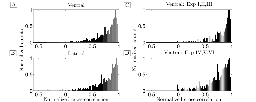
Figure 12: Histograms of signal correlation between the estimated RP and the GT. (A) RP ventral Vs. GT, (B) RP lateral Vs. GT, (C) RP ventral Vs. GT for experiments (I, II, III), (D) RP ventral Vs. GT for experiments (IV, V VI).

Also, it is seen that the skewness of the histogram for experiments IV, V and VI is worse than that for experiments I, II and III as indicated in Fig. 12 (C and D). This is because the generating signals corresponding to experiments IV, V and VI have time-varying frequency components. However, note that for the case in which only spectral magnitudes vary with time but not frequency values, the theoretical results and performance of the proposed method remains unaltered.

Figure 10 depicts a scene from one of the experiments on a subject, with the selected membership set ($X^{+}$) marked with red dots. It is seen that the selected pixels are not geographically contiguous and mostly in the abdominal-thoracic region of the subject where the respiratory movement is significantly manifested. It is also possible that there can be a small number of very low SNR pixels that get assigned to $X^{+}$ because of the effect of noise-cloud explained in Sec. II. E. The LTI channels corresponding to these pixels do not contain significant respiratory information (for instance, red points on the wall in lateral view of Fig. 10). However, these points often do not alter the estimate as, often, they are very small in number compared to the pixels that have significant signal components and thus get nullified while ensemble averaging. The algorithm allows further control over such instances through the choice of parameter GoE and hence radius of exclusion ($r_{e}$).

The aforementioned performance of the algorithm seems significant given that the experiments involve the following: (i) random textured clothing on subjects, (ii) camera of two different resolutions and positions, (iii) six different breathing patterns. In conclusion, it is observed that the proposed algorithm offers a good estimate of the RP (and RR) if the camera is placed in the ventral position with a clothing that has a texture with some region of similar patterns.

III-C Robustness aspects

In this section, we discuss the robustness of the proposed method for the cases where there are deviations from the assumed models and discuss its noise tolerance for the application considered.

1. Amplitude modulation - Suppose the generating signal $g(t)$ is modulated with a slowly time-varying modulating signal $m(t)$, that is, $g(t)=m(t)\sum\limits_{k=1}^{N}G_{k}sin(w_{k}t+\theta)$. For such signals, it can be easily shown that the results developed in Sec. II remain valid. An intuitive understanding of this fact may be inferred from noticing that the estimate proposed here has an arbitrariness in the amplitude scale of the estimated signal. Thus, in case of amplitude modulation, the estimated signal remains to be the actual generating signal up to an arbitrary constant scaling factor. This fact is corroborated with the results of experiments IV, V and VI on the real-life data set, which have amplitude modulating components in them.

2. Frequency modulation - Suppose the generating signal is frequency modulated, that is, $g(t)=\sum\limits_{k=1}^{N}G_{k}sin(w_{k}(t)t+\theta)$ where $w_{k}(t)$ is slowly varying. For this case, the results developed in Sec. II, do not extend directly. This is because of two reasons: (a) frequency modulated signals do not adhere to the periodicity assumption that is imposed on the generating signal during the development of the theory, (b) the basis vectors on which the signals are projected are a function of fundamental frequency required to be a constant (Eq. 9 and 10). However the proposed method can be modified to retain approximate validity for the case where the generating signals are quasi-periodic, that is, $w_{k}(t)$ is slowly varying.A straightforward extension of the proposed method for this category of signals is to recompute $X^{+}$ at regular short intervals (governed by the assumed interval of the quasi-periodicity). This method is shown to yield considerably good estimates of the signal morphology in the cases of the real-data for the cases of experiments IV, V and VI where the generating signal resembles a quasi-stationary frequency modulated signal.

3. Tolerance to sporadic body-movement and background disturbances - In practical scenarios, there will be movements in the human body that do not correspond to respiratory motion. In addition, there can also be movements caused by objects other than the human body. If such movements impact only the pixels that are not contained in $X^{+}$, the performance of the method remains unaltered. In the event such movement influences pixels within $X^{+}$, it has been observed that the ensemble averaging retains robust performance provided such motion impacts a smaller fraction of $X^{+}$. This fact has also been corroborated with the results on the real-life data set where the subjects were not strictly constrained to be still but there were asked to breath sitting in a relaxed posture.

Given the aforementioned discussions, some of the major merits of the proposed method may be listed as follows - (a) it is a generic framework for blind-deconvolution of SIMO systems driven by periodic inputs without the need for estimating the underlying channel responses, noise characteristics or error minimization making the method asymptotically exact when there is no noise, (b) when applied to respiration pattern estimation, this method selects a set of most-relevant pixels that would estimate the signal which need not be geographically continuous and thus does not critically depend on ROI selection, camera orientation and texture of the surface, (c) it is computationally inexpensive and thus can be implemented in real-time. Nevertheless, the proposed estimator is limited by (a) its inability to quantify true magnitude of the generating signal and (b) its non-applicability to the class of signals with rapidly varying time-frequency components.

IV Conclusion and future work

In this paper, we proposed a generic blind deconvolution framework to extract periodic signals from videos. A video is modeled as an ensemble of LTI measurement channels all driven by a single generating signal. No assumptions are made on the characteristics of the individual channels except for IID randomness. A simple ensemble averaging over a carefully selected membership set is proposed as an effective estimator which is shown to converge to the generating signal under minimally restrictive assumptions. A method for grouping the channels to obtain the optimal membership set based on the location of the coefficients of the quadratic fits of the LTI channel responses is described. This framework is applied on the problem of non-contact respiration pattern estimation using videos and it is shown to yield comparable results with a medical gold-standard device namely impedance pneumograph. Our future work is aimed at extending this framework to (i) deal with signals having rapidly varying time-frequency components, (ii) estimate other relevant biomedical signals from video and (iii) deal with significant sources of motion other than the one caused by the desired source.

References

- [1] J. B. Institute et al., “Vital signs,” Management in Health, vol. 11, no. 4, 2009.
- [2] “WHO strategy for prevention and control of chronic respiratory diseases.”
- [3] F. Yasuma and J.-i. Hayano, “Respiratory sinus arrhythmia: why does the heartbeat synchronize with respiratory rhythm?” Chest Journal, vol. 125, no. 2, pp. 683–690, 2004.
- [4] H. D. Kubo and B. C. Hill, “Respiration gated radiotherapy treatment: a technical study,” Physics in medicine and biology, vol. 41, no. 1, p. 83, 1996.
- [5] M. R. Miller et al., “Standardisation of spirometry,” European respiratory journal, vol. 26, no. 2, pp. 319–338, 2005.
- [6] L. Geddes et al., “The impedance pneumography.” Aerospace medicine, vol. 33, pp. 28–33, 1962.
- [7] K. Nakajima et al., “Monitoring of heart and respiratory rates by photoplethysmography using a digital filtering technique,” Medical engineering & physics, vol. 18, no. 5, pp. 365–372, 1996.
- [8] P. T. Macklem et al., “Phonospirometry for non-invasive monitoring of respiration,” Jun. 5 2001, US Patent 6,241,683.
- [9] C.-L. Que et al., “Phonospirometry for noninvasive measurement of ventilation: methodology and preliminary results,” Journal of Applied Physiology, vol. 93, no. 4, pp. 1515–1526, 2002.
- [10] R. Murthy and I. Pavlidis, “Noncontact measurement of breathing function,” Engineering in Medicine and Biology Magazine, IEEE, vol. 25, no. 3, pp. 57–67, 2006.
- [11] F. Al-khalidi et al., “Tracing the region of interest in thermal human face for respiration monitoring,” International Journal of Computer Applications, vol. 119, no. 4, 2015.
- [12] W. Verkruysse et al., “Remote plethysmographic imaging using ambient light.” Optics express, vol. 16, no. 26, pp. 21 434–21 445, 2008.
- [13] K. H. Chon et al., “Estimation of respiratory rate from photoplethysmogram data using time–frequency spectral estimation,” IEEE Transactions on Biomedical Engineering, vol. 56, no. 8, pp. 2054–2063, 2009.
- [14] M.-Z. Poh et al., “Advancements in noncontact, multiparameter physiological measurements using a webcam,” IEEE Transactions on Biomedical Engineering, vol. 58, no. 1, pp. 7–11, 2011.
- [15] ——, “Non-contact, automated cardiac pulse measurements using video imaging and blind source separation.” Optics express, vol. 18, no. 10, pp. 10 762–10 774, 2010.
- [16] W. Wang et al., “Exploiting spatial redundancy of image sensor for motion robust rppg,” IEEE Transactions on Biomedical Engineering, vol. 62, no. 2, pp. 415–425, 2015.
- [17] S. G. Fleming and L. Tarassenko, “A comparison of signal processing techniques for the extraction of breathing rate from the photoplethysmogram,” Int J Biol Med Sci, vol. 2, no. 4, pp. 232–6, 2007.
- [18] S. D. Min et al., “Noncontact respiration rate measurement system using an ultrasonic proximity sensor,” IEEE Sensors Journal, vol. 10, no. 11, pp. 1732–1739, 2010.
- [19] T. Kondo et al., “Laser monitoring of chest wall displacement,” European Respiratory Journal, vol. 10, no. 8, pp. 1865–1869, 1997.
- [20] M. Mabrouk et al., “Model of human breathing reflected signal received by pn-uwb radar,” in Engineering in Medicine and Biology Society (EMBC), 2014 36th Annual International Conference of the IEEE. IEEE, 2014, pp. 4559–4562.
- [21] C. Gu and C. Li, “Assessment of human respiration patterns via noncontact sensing using doppler multi-radar system,” Sensors, vol. 15, no. 3, pp. 6383–6398, 2015.
- [22] M.-C. Yu et al., “Noncontact respiratory measurement of volume change using depth camera,” in Engineering in Medicine and Biology Society (EMBC), 2012 Annual International Conference of the IEEE. IEEE, 2012, pp. 2371–2374.
- [23] F. Benetazzo et al., “Respiratory rate detection algorithm based on rgb-d camera: theoretical background and experimental results,” Healthcare technology letters, vol. 1, no. 3, p. 81, 2014.
- [24] E. A. Bernal et al., “Non contact monitoring of respiratory function via depth sensing,” in IEEE-EMBS International Conference on Biomedical and Health Informatics (BHI). IEEE, 2014, pp. 101–104.
- [25] D. Shao et al., “Noncontact monitoring breathing pattern, exhalation flow rate and pulse transit time,” IEEE Transactions on Biomedical Engineering, vol. 61, no. 11, pp. 2760–2767, 2014.
- [26] K.-Y. Lin et al., “Image-based motion-tolerant remote respiratory rate evaluation,” IEEE Sensors Journal, vol. 16, no. 9, pp. 3263–3271, 2016.
- [27] R. Janssen et al., “Video-based respiration monitoring with automatic region of interest detection,” Physiological measurement, vol. 37, no. 1, p. 100, 2015.
- [28] C. Avishek et al., “Real-time respiration rate measurement from thoracoabdominal movement with an inexpensive consumer grade camera,” in Engineering in Medicine and Biology Society (EMBC), 2016 38th Annual International Conference of the IEEE, accepted for publication.
- [29] L. Zhang, A. Cichocki, and S.-i. Amari, “Multichannel blind deconvolution of nonminimum-phase systems using filter decomposition,” IEEE Transactions on Signal Processing, vol. 52, no. 5, pp. 1430–1442, 2004.
- [30] J. Makhoul, “Linear prediction: A tutorial review,” Proceedings of the IEEE, vol. 63, no. 4, pp. 561–580, 1975.
- [31] D. Kundur and D. Hatzinakos, “A novel blind deconvolution scheme for image restoration using recursive filtering,” IEEE Transactions on Signal Processing, vol. 46, no. 2, pp. 375–390, 1998.
- [32] E. Moulines, P. Duhamel, J.-F. Cardoso, and S. Mayrargue, “Subspace methods for the blind identification of multichannel fir filters,” IEEE Transactions on signal processing, vol. 43, no. 2, pp. 516–525, 1995.
- [33] L. Tong, G. Xu, and T. Kailath, “Blind identification and equalization based on second-order statistics: A time domain approach,” IEEE Transactions on information Theory, vol. 40, no. 2, pp. 340–349, 1994.
- [34] N. S. Johnston, R. Light, J. Zhang, M. Somekh, and M. Pitter, “2d cmos image sensors for the rapid acquisition of modulated light and multi-parametric images,” in SPIE Optics+ Optoelectronics. International Society for Optics and Photonics, 2011, pp. 807 303–807 303.
- [35] E. R. Fossum et al., “Cmos image sensors: electronic camera-on-a-chip,” IEEE transactions on electron devices, vol. 44, no. 10, pp. 1689–1698, 1997.
- [36] M. El-Desouki, M. Jamal Deen, Q. Fang, L. Liu, F. Tse, and D. Armstrong, “Cmos image sensors for high speed applications,” Sensors, vol. 9, no. 1, pp. 430–444, 2009.
- [37] A. F. Pacela, “Impedance pneumography-a survey of instrumentation techniques,” Medical and biological engineering, vol. 4, no. 1, pp. 1–15, 1966.
- [38] J. Benesty et al., “Pearson correlation coefficient,” in Noise reduction in speech processing. Springer, 2009, pp. 1–4.
- [39] J. M. Bland and D. Altman, “Statistical methods for assessing agreement between two methods of clinical measurement,” The lancet, vol. 327, no. 8476, pp. 307–310, 1986.