The importance of being consistent.

Abstract

We review the role of self-consistency in density functional theory. We apply a recent analysis to both Kohn-Sham and orbital-free DFT, as well as to Partition-DFT, which generalizes all aspects of standard DFT. In each case, the analysis distinguishes between errors in approximate functionals versus errors in the self-consistent density. This yields insights into the origins of many errors in DFT calculations, especially those often attributed to self-interaction or delocalization error. In many classes of problems, errors can be substantially reduced by using ‘better’ densities. We review the history of these approaches, many of their applications, and give simple pedagogical examples.

1 Introduction

Density functional theory(DFT) is used in more than 30,000 scientific papers per yearPGB15 (PJGB15). Most of these applications are routine, where the calculation yields sufficiently accurate results as to provide insight into some scientific or technological problem. Most use the Kohn-Sham (KS) scheme with one of a very small set of popular functional approximations whose successes and failures are well-documented. For example, the standard approximations are ‘known’ to fail when there is substantial self-interaction or strong correlation or localization in the systemMCY08 (MSCY08). These concepts are closely related to one another.

Partition-DFT (PDFT) is an exact generalization of DFT using fragment densities as the basic variablesCW07 (CW07). Many difficulties of KS-DFT are overcome by PDFT. PDFT can deal with strong correlation; it allows for extremely chemical interpretations of DFT calculations; it provides a direct route to energy differences, not only total energies; and it is well suited for linear-scaling implementations and parallelization.

Almost all DFT calculations employ a basic principle that was used in the original Thomas-Fermi theoryT27 (Tho27, Fer28). When one constructs an approximation to the energy as a functional of the density, one then uses it to find the density for that system, by minimizing the approximate energy. This is true of the exact functional, and is used in almost all practical DFT calculations with approximate functionals. With such a choice, basic theorems such as the Hellmann-Feynman theorem apply, allowing easy calculation of forces, etc.

This principle appears so common-sensical that it is difficult to question. Surely you get the most accurate energy by minimization? In fact, this is not always the case. We examine the errors made by self-consistency and find that, in certain, well-defined, common situations, the errors made in the density overwhelm those made in the evaluation of the functional, and often these can be fixed with little additional computational effort.

We also apply our enery-error analysis to PDFT, showing that several of the key concepts in PDFT are, in fact, the same as those involved in energy-error analysis, and how both can be employed to understand the remaining errors in PDFT.

Figure 1: Binding energy curves of H${}_{2}^{+}$. Black is exact, blue is self-consistent PBE, blue-dashed is PBE on HF density, and red is approximate PDFT, Equation 25. Energies are in eV.

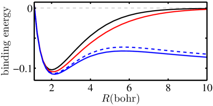
Throughout this article, we use the H${}_{2}^{+}$ binding energy curve to illustrate many concepts and approximations involved. In Figure 1, the black line is the exact curve, given by a Hartree-Fock (HF) calculation, while the blue line is for a standard DFT calculationPBE96 (PBE96), showing the infamous failure as the bond is stretchedMCY08 (MSCY08). The blue-dashed line is from HF-DFT, meaning the DFT calculation on the HF density. While this method cures many problems with standard DFT, it has almost no effect here, because the bond is symmetric. On the other hand, a simple approximation within PDFT (Section2.2.4 within) yields a tremendous improvement over standard DFT. The rest of this review explains how.

2 Background

We restrict ourselves to non-relativistic systems within the Born-Oppenheimer approximation with collinear magnetic fieldsED11 (ED11). DFT is concerned with efficient methods for finding the ground-state energy and density of $N$ electrons whose Hamiltonian is

$$\hat{H}=\hat{T}+\hat{V}_{\rm ee}+\hat{V},~{}~{}~{}\hat{V}=\sum_{i=1}^{N}v({\bf r}_{i}).$$ (1)

The first of these is the kinetic energy operator, the second is the electron-electron repulsion, while the last is the one-body potential. Only $N$ and $v({\bf r})$ change from one system to another, be they atoms, molecules or solids. We use atomic units throughout, unless otherwise stated.

2.1 Standard DFT

2.1.1 Pure DFT

In 1964, Hohenberg and Kohn(HK)HK64 (HK64) proved that, for a given electron-electron interaction, there was at most one $v({\bf r})$ that could give rise to the ground-state one-particle density $n({\bf r})$ of a system. If we write L79 (Lev79, Lie83)

$$F[n]=\min_{\Psi\to n}\langle\Psi|\,\hat{T}+\hat{V}_{\rm ee}\,|\Psi\rangle=T[n]+V_{\rm ee}[n],$$ (2)

where the minimization is over all normalized, antisymmetric $\Psi$ with one-particle density $n({\bf r})$, then

$$E=\min_{n}\left\{F[n]+\int d^{3}r\,n({\bf r})\,v({\bf r})\right\}.$$ (3)

The Euler equation corresponding to the above minimization for fixed $N$ is simply

$$\frac{\delta F[n]}{\delta n({\bf r})}=-v({\bf r}).$$ (4)

Armed with the exact $F[n]$, the solution of this equation yields the exact ground-state density which, when inserted back into $F[n]$, yields the exact ground-state energy.

This theorem proved that the original, crude DFT of Thomas and FermiT27 (Tho27, Fer28) was an approximation to an exact approach. Back then, they approximated

$$T[n]\simeq T^{\rm TF}[n]=\frac{3(3\pi^{2})^{2/3}}{10}\int d^{3}r\ n^{5/3}({\bf r}),$$ (5)

and $V_{\rm ee}$ with the Hartree energy, the classical self-repulsion of the charge density

$$V_{\rm ee}[n]\simeq U_{\scriptscriptstyle\rm H}[n]=\frac{1}{2}\int d^{3}r\,\int d^{3}r^{\prime}\,\frac{n({\bf r})\,n({\bf r}^{\prime})}{|{\bf r}-{\bf r}^{\prime}|}.$$ (6)

Adding these together to approximate $F$ yields the iconic Thomas-Fermi(TF) theory, and the Euler equation for an atom yields the TF density of atoms. This approximation yields energies that are good to within about 10%, but since, e.g., all thermochemistry depends on very tiny differences in electronic energies, TF theory is not accurate enough for chemical or modern materials science applications.

2.1.2 Kohn-Sham DFT

To increase accuracy and construct $F[n]$, modern DFT calculations use the KS scheme that imagines a fictitious set of non-interacting electrons with the same ground-state density as the real HamiltonianKS65 (KS65). These electrons satisfy the KS equations:

$$\left\{-\frac{1}{2}\nabla^{2}+v_{\scriptscriptstyle\rm S}({\bf r})\right\}\,\phi_{i}({\bf r})=\epsilon_{i}\,\phi_{i}({\bf r}),$$ (7)

where $v_{\scriptscriptstyle\rm S}({\bf r})$ is defined as the unique potential such that $n({\bf r})=\sum_{occ}\,|\phi_{i}({\bf r})|^{2}$. To relate these to the interacting system, we write

$$F[n] = T_{\scriptscriptstyle\rm S}[n]+E_{\scriptscriptstyle\rm HXC}[n],$$

$$T_{s}[n] = \frac{1}{2}\int d^{3}r\,\sum_{i=1}^{N}|\nabla\phi_{i}({\bf r})|^{2},$$ (8)

where $T_{\scriptscriptstyle\rm S}$ is the non-interacting (or KS) kinetic energy, assuming the KS wavefunction (as is usually the case) is a single Slater determinant. Here $E_{\scriptscriptstyle\rm HXC}=U_{\scriptscriptstyle\rm H}+E_{\scriptscriptstyle\rm XC}$ is the sum of the Hartree and exchange-correlation (XC) energies and is defined by Equation 8. Lastly, we differentiate Equation 8 with respect to the density, yielding

$$v_{\scriptscriptstyle\rm S}({\bf r})=v({\bf r})+v_{\scriptscriptstyle\rm HXC}({\bf r}),~{}~{}~{}v_{\scriptscriptstyle\rm HXC}({\bf r})=\frac{\delta E_{\scriptscriptstyle\rm HXC}}{\delta n({\bf r})}.$$ (9)

This is the single most important result in DFT, as it closes the set of KS equationsKS65 (KS65). Since $U_{\scriptscriptstyle\rm H}$ is known as an explicit density functional (Equation 6) given any expression for $E_{\scriptscriptstyle\rm XC}$ in terms of $n({\bf r})$, either approximate or exact, the KS equations can be solved self-consistently to find $n({\bf r})$ for a given $v({\bf r})$. The self-consistency is simply finding the minimum of an approximate $F$ determined from an approximate $E_{\scriptscriptstyle\rm XC}$.

Figure 2: ExactUG94 (UG94) and approximate DFT densities and KS potentials of the He atom, using PBE, PBE0 and exact exchange, in a.u. The dashed horizontal lines indicate the eigenvalues of the 1s orbitals.

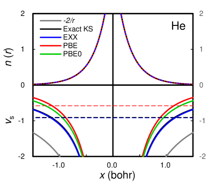
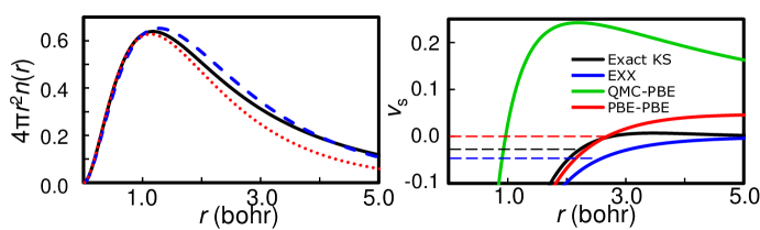
In Figure 2, we show the exact $v_{\scriptscriptstyle\rm S}({\bf r})$ of the He atom, found by inverting Equation 7 after finding a highly accurate density by solving the Schrödinger equationUG94 (UG94). Inserting two non-interacting KS electrons in the 1s orbital of $v_{\scriptscriptstyle\rm S}({\bf r})$ yields the exact $n({\bf r})$. All practical KS-DFT calculations approximate $v_{\scriptscriptstyle\rm S}({\bf r})$. The $1s$ HOMO is at precisely $-I$, where $I$ is the ionization energy. The energies and eigenvalues for both He and H^-, both exactly, given by quantum Monte-Carlo(QMC) densities, and approximately, are given in Table I.

Table 1: Energies for He and H^- in Hartree.

atom	$E$			$E_{{}^{\rm PBE}}[n]$		$\Delta E_{{}^{\rm PBE}}\times 1000$			$\epsilon^{\rm HOMO}$
	Exact	HF	PBE	$n_{\rm HF}$	$n_{\rm QMC}$	$\Delta E$	$\Delta E_{F}$	$\Delta E_{D}$	exact	HF	PBE
He	-2.904	-2.862	-2.893	-2.892	-2.892	10.8	11.8	-1.0	-0.903	-0.918	-0.579
H-	-0.528	-0.488	-0.538	-0.521	-0.527	-10.4	1.0	-11.4	-0.028	-0.046	-0.000

Many forms of approximation exist for $E_{\scriptscriptstyle\rm XC}[n]$, the most popular being the generalized gradient approximation (GGA)P86 (Per86, Bec88, LYP88, Per+92, PBE96), and hybrids of GGA with exact exchange from a HF calculationB93 (Bec93, PEB96, AB99, HSE03),

$$E_{\scriptscriptstyle\rm XC}^{\rm GGA} = \int d^{3}r\ e_{\scriptscriptstyle\rm XC}^{\rm GGA}(n({\bf r}),|\nabla n({\bf r})|),$$

$$E_{\scriptscriptstyle\rm XC}^{\rm hyb} = a\,(E_{\scriptscriptstyle\rm X}-E_{\scriptscriptstyle\rm X}^{\rm GGA})+E_{\scriptscriptstyle\rm XC}^{\rm GGA}.$$ (10)

Here $a$ is the fixed mixing parameter, usually chosen between about 0.2 and 0.25 to optimize energetics for a large range of molecular dissociation energiesB93 (Bec93, PEB96). All practical calculations generalize the preceding formulas for arbitrary spin using spin-DFT BH72 (BH72). The computational ease of DFT calculations relative to more accurate wavefunction methods usually allows much larger systems to be calculated, leading to DFT’s immense popularity todayPGB15 (PJGB15). However, all these approximations fail in the paradigm case of stretched H₂, the simplest example of a strongly correlated systemB01 (Bae01).

For just one particle, we know the explicit functionals:

$$T_{\scriptscriptstyle\rm S}=\int d^{3}r\,\frac{|\nabla n|^{2}}{8n},~{}~{}~{}E_{\scriptscriptstyle\rm X}=-U_{\scriptscriptstyle\rm H},~{}~{}~{}E_{\scriptscriptstyle\rm C}=0,~{}~{}(N=1).$$ (11)

None of the popular functionals satisfy these conditions for all one-electron systems, and their errors are called self-interaction errors (SIE).

In Figure 2, $v_{\scriptscriptstyle\rm S}^{\rm PBE}({\bf r})$ is substantially above the exact curve, and its HOMO level is several eV too high (Table I), but the almost constant shift in $v_{\scriptscriptstyle\rm S}({\bf r})$ has little effect on $n({\bf r})$ and therefore on $E$. Note also that the HF potential is very close to the true potential, and suffers none of the difficulties of standard approximations. But the hybrid functionals have potentials that are essentially those of GGA with $a$ times the HF potential mixed in, so their $\epsilon_{i}$ tend to have an error that is about a fraction $a$ smaller than that of their GGA counterparts, i.e., still large, as in the PBE0 curve of Figure 2. Many of these concepts are described more precisely these days with the notion of delocalization errorLZCM15 (Li+15, Zhe+15). These localization effects become more subtle in polarizable solvent modelsDJ15 (DJ15), and are especially important in Na-water clustersSRR15 (SRR15).

Later, we explain how such popular approximations for the energy can have such ‘bad’ potentials, yet yield such useful energetics.

2.2 Partition DFT

Most codes based on KS-DFT scale as $N^{3}$, with $N$ an appropriate measure of the size of the system. This is a very significant improvement over correlated wavefunction-based methods, but still impractical for large systems. DFT-based Car-Parrinello optimizations, for example, are limited to systems of no more than a few thousand atoms. In response to this challenge, linear-scaling schemes have been developed G99 (G9̈9). Some of these take advantage of the nearsightedness of electronic properties SK66 (SK66, Yip91). Other schemes break the system into fragments that are small enough for rapid computation, and then build the properties of the whole system in a way which preserves order-$N$ scaling NG04 (NG04, FK07). Since the unfavorable scaling of KS-DFT arises primarily from the use of KS orbitals, orbital-free schemes have also been developed that perform direct minimization of the energy functional and scale linearly with $N$ WC00 (WC00, HC09). The quasicontinuum-DFT approach (QCDFT) PZHC08 (Pen+08), combining the coarse-graining idea of multiscale methods CLK05 (Cho+05) with the coupling strategy of QM/MM (Quantum-Mechanics / Molecular-Mechanics) SHFM96 (Sve+96, GT02, FG05), allows for the simulation of multimillion atoms via orbital-free DFT embedding. Explicit treatment of a few million atoms has been demonstrated via linear-scaling orbital-free DFT algorithms HC09 (HC09, Che+16). These, however, rely on approximations to the non-interacting kinetic energy functional $T_{s}[n]$, which are neither sufficiently accurate nor general.

PDFTCW07 (CW07, Ell+10) is an exact reformulation of DFT with the potential to overcome both problems of scaling with system size and problems related to errors made by the approximate XC functionals. PDFT was developed initially to strenghten the foundations of chemical reactivity theory CW07 (CW07, CW03). Its structure belongs to the family of density-based embedding methods that were developed starting in the early 1970’s to improve the efficiency of electronic-structure calculations via fragmentation. PDFT generalizes all aspects of both pure and KS-DFT with new variables that have an extremely chemical interpretation, while also providing all the computational advantages of quantum embedding methods. Because excellent, comprehensive reviews on embedding have appeared recently JN14 (JN14, Kri+15, WSZ15), we list only a few highlights relevant to this review.

2.2.1 A few quantum embedding highlights

1970’s: Based on the assumption that the density of rare-gas dimers can be well approximated by the sum of their isolated-atom densities, the first non self-consistent embedding calculations of the binding-energy curves of rare-gas dimers were performed by Gordon and Kim(GK method). GK72 (GK72).

1980’s: Corrections were added to the non-self consistent GK calculations to account for self-interaction errors WP81 (WP81) and to include induction effects and dispersion forces H84 (Har84). The first self-consistent versions of the GK model were also proposed SS86 (SS86).

1990’s: Subsystem-DFT (S-DFT) C91 (Cor91) and frozen-density embedding (FDE) WW93 (WW93) were developed. FDE was initially not completely self-consistent, but was later made self-consistent via freeze-and-thaw cycles, making it equivalent to S-DFT. The self-consistent atomic deformation theory (SCAD) is a version of S-DFT requiring the fragment densities to be written as atomic densities BM93 (BM93). Other methods treat different fragments with different levels of theory, allowing for critical fragments of a larger calculation to be treated with higher accuracy (usually referred to as embedding-DFT). In all cases, the main equations are the KS equations with constrained electron density (KSCED) WW96 (WW96).

2000’s: Many developments took place, mostly of a technical nature HC08 (HC08): FDE was applied with a plane-wave basis and both local and non-local pseudopotentials TB00 (TB00); the idea of buffer fragments was introducedCW04 (CW04); FDE was extended to time-dependent DFT (TDDFT) Wes04 (Wes04, Neu+05, Neu07) and to work in combination with configuration-interaction methods KGWC02 (Klü+02). In parallel, significant advances were made for computational sampling procedures in QM/MM KHW09 (KHW09).

2010’s: New methods can now calculate $\delta T_{{}_{\scriptscriptstyle\rm S}}^{\rm nad}/\delta n(r)$ for covalent bonds FJNV10 (Fux+10), or bypass the need for inversions altogether via exact density embedding MSGM12 (Man+12); FDE develops to study charge-transfer reactions PN11 (PN11), calculate charge-transfer excitation energies and diabatic couplings PVVN13 (Pav+13), and include van der Waals interactions KEP14 (KEP14). Much is now known about the performance of approximate self-consistent S-DFT SKMV15 (Sch+15). Sources of error in WFT-in-DFT embedding was investigated GBMMI14 (Goo+14).

2.2.2 PDFT in a nutshell

Although PDFT has been extended to the time-dependent case MJW13 (MJW13, MW14, MW15), we focus here on the ground-state theory, where the goal is to calculate $E$ and $n({\bf r})$ of a molecule via fragment calculations. The user chooses how the nuclei are assigned into fragments by dividing the one-body potential. For simplicity, we give formulas for just two fragments, but there can be as many as desired. Here

$$v({\bf r})=v_{1}({\bf r})+v_{2}({\bf r}).$$ (12)

The choice of $\{v_{1},v_{2}\}$, together with $N$, unambiguously determine a unique, global partition potential $v_{p}({\bf r})$ and a unique set of fragment densities CW06 (CW06): ${\bf n}=(n_{1}({\bf r}),n_{2}({\bf r}))$. Each resulting $n_{\alpha}({\bf r})$ is the ground-ensemble density of $N_{\alpha}$ electrons in $v_{\alpha}({\bf r})+v_{p}({\bf r})$, with $N_{1}+N_{2}=N$. At self-consistency, $v_{p}({\bf r})$ is global (independent of $\alpha$), and

$$n_{1}({\bf r})+n_{2}({\bf r})=n({\bf r}).$$ (13)

We omit here spin indices for notational simplicity (but see MW13 (MW13, NW14)). The self-consistent equations that are solved to find $\bf n$ and the partition potential $v_{p}({\bf r})$ follow from the Euler equation of a constrained minimization. The quantity being minimized is not the total energy of the molecule, as in standard FDE and S-DFT, but rather

$$E_{\rm frag}[{\bf n}]=E_{1}[n_{1}]+E_{2}[n_{2}],$$ (14)

the sum of the fragment energies, where $E_{\alpha}[n]$ is the ground-state energy functional for potential $v_{\alpha}({\bf r})$. If $N_{1}$ is not an integer, then write $N_{1}=M+\nu$, $0\leq\nu<1$, and PPLB82 (Per+82):

$$E_{1}[n] = (1-\nu)E_{1}[n_{M}]+\nu E_{1}[n_{M+1}],$$

$$n_{1}({\bf r}) = (1-\nu)n_{M}({\bf r})+\nu n_{M+1}({\bf r}).$$ (15)

Thus, only integer calculations need be performed, but $E_{\rm frag}[{\bf n}]$ is minimized with respect to $\nu$ as well, so $N_{1}$ need not be an integer.

The formal constraints under which $E_{\rm frag}[{\bf n}]$ is minimized are Equation 13 and the number constraint $N=N_{1}+N_{2}$. The partition potential $v_{p}({\bf r})$ and the chemical potential $\mu$ can be seen as the Lagrange multipliers guaranteeing these constraints. Writing $E_{1,2}[n]$ in terms of KS quantities, this constrained minimization leads to the KS-PDFT equationsEBCW10 (Ell+10) which, for a given approximation to the $\rm XC$ functional, exactly reproduce the results of the corresponding KS calculation for the entire system (using the same $\rm XC$ functional). At the minimum, $E_{\rm frag}[{\bf n}]$ differs from the true energy by the partition energy $E_{p}[{\bf n}]$, whose functional derivative evaluated at any minimizing $n_{\alpha}({\bf r})$ is the partition potential:

$$E_{p}[{\bf n}]\equiv E[n]-E_{\rm frag}[{\bf n}],~{}~{}v_{p}({\bf r})=\frac{\delta E_{p}}{\delta n_{1}({\bf r})}=\frac{\delta E_{p}}{\delta n_{2}({\bf r})}.$$ (16)

As in S-DFT, the partition energy is divided into the non-additive Kohn-Sham components:

$$E_{p}[{\bf n}]=F^{\rm nad}[{\bf n}]+V^{\rm nad}[{\bf n}]$$ (17)

where $F^{\rm nad}[{\bf n}]=F[n_{1}+n_{2}]-F[n_{1}]-F[n_{2}]$. In Equation 17, $V^{\rm nad}$ includes both the non-additive electron-nuclear and nuclear-nuclear interactions. The calculation requires either an explicit density-functional approximation for $T_{s}^{\rm nad}[{\bf n}]$, as in Ref.WEW98 (WEW98), or (computationally expensive) inversions, as in Ref.GAMM10 (Goo+10). If one only minimizes $E[n]$, this non-additive term may be made to vanish by requiring that orbitals from different fragments are orthogonal to each otherMSGM12 (Man+12). This, however, requires a molecular KS calculation ahead of time.

Figure 3: Partitioned energy contributions to binding curve of H${}_{2}^{+}$. The dissociation curve ($E_{\rm dis}$, solid) is the difference between the partition energy ($E_{p}$, dotted, $1/R$ included) and the relaxation energy ($E_{\rm rel}$, dashed), Equation 19. Black are exact, blue are PBE, red are the overlap approximation.

Why minimize $E_{\rm frag}[{\bf n}]$ (Equation 14) rather than the total energy directly? With the constraint of Equation 13, the answer is clear: When $n({\bf r})$ is the true ground-state density, the HK theorem guarantees that we have also minimized $E[n]$, and produced “chemically meaningful” fragmentsRP86 (RP86). The total work done in deforming the isolated fragment densities to produce the PDFT fragment densities is the relaxation energy $E_{\rm rel}$,

$$E_{\rm rel}=E_{\rm frag}^{(\infty)}-E_{\rm frag},$$ (18)

where $E_{\rm frag}^{(\infty)}$ is the sum of the fragment energies when the fragments are infinitely separated from each other. (In the original GK model GK72 (GK72), $E_{\rm rel}=0$.) The true dissociation energy of the system, $E_{\rm dis}=E-E_{\rm frag}^{(\infty)}$ is related to the partition energy, Equation 16, by:

$$E_{p}=E_{\rm rel}+E_{\rm dis}.$$ (19)

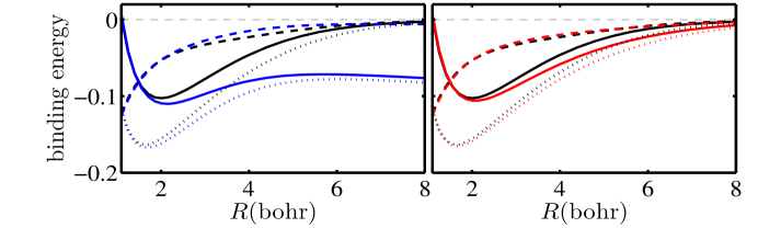
In Figure 3, we show the exact contributions and their PBE counterparts. Both $E_{\rm rel}$ and $E_{p}$ contribute substantially at equilibrium. Clearly, the failure of PBE is primarily in $E_{p}$.

The partition trick is thus analogous to the KS trick: The former maps the system into isolated fragments, while the latter maps the system to non-interacting electronsN15 (Naf15). In KS-DFT, the self-consistent density from solution of the KS equations is also that which minimizes $E[n]$. The KS “density constraint” guarantees this, by construction. Furthermore, $v_{p}({\bf r})$ in PDFT, like $v_{\scriptscriptstyle\rm HXC}({\bf r})$ in KS-DFT, is a global potential that is added to $v({\bf r})$ to make the auxiliary system. It is unique for a choice of partitioning, as follows from the minimization of $E_{\rm frag}[{\bf n}]$ CW06 (CW06). In this analogy, PDFT is to subsystem-DFT like KS-DFT is to Hartree-Fock theory.

2.2.3 In practice: Converging to self-consistency

For each fragment $\alpha$, two KS-like equations are solved simultaneously:

$$\left\{-\frac{1}{2}\nabla^{2}+v_{\alpha}^{\rm eff}[n_{\alpha}^{\pm}]({\bf r})+v_{p}({\bf r})\rm\right\}\phi_{i,\alpha}^{\pm}({\bf r})=\epsilon^{\pm}_{i,\alpha}\phi^{\pm}_{i,\alpha}({\bf r}),$$ (20)

where the effective potential is just the usual KS form, Equation 9, and $\pm$ denotes evaluation for $M$ and $M+1$ electrons. The various partition potentials generally differ until a self-consistent solution is reached. For a given set of trial fragment densities, define

$$v_{p,\alpha}^{\pm}({\bf r})=\delta E_{p}[{\bf n}]/\delta n^{\pm}_{\alpha}({\bf r}).$$ (21)

We construct a weighted average partition potential over all fragments and particle numbers:

$$v_{p}({\bf r})=\int d^{3}r^{\prime}\,\sum_{\alpha=1}^{2}\,\sum_{\lambda=\pm}\,v_{p,\alpha}^{\lambda}({\bf r}^{\prime})\,Q^{\lambda}_{\alpha}({\bf r}^{\prime},{\bf r}).$$ (22)

The $Q$-functions provide the bridge between PDFT and S-DFT calculationsNW14 (NW14), and are approximated in practice asMW13 (MW13):

$$Q^{\lambda}_{\alpha}({\bf r}^{\prime},{\bf r})=\frac{\delta n^{\lambda}_{\alpha}({\bf r}^{\prime})}{\delta n_{\rm frag}({\bf r})}\approx\frac{n_{\alpha}^{\lambda}({\bf r})}{n_{\rm frag}({\bf r})}\delta({\bf r}-{\bf r}^{\prime})~{}~{}.$$ (23)

In Equation 23, $n_{\rm frag}({\bf r})$ is the sum of trial fragment densities at intermediate iterations, equal to the correct molecular density only at convergence. When the exact partition energy is used, either via iterative inversionsNWW11 (NWW11) or through use of the exact $T_{\scriptscriptstyle\rm S}[n]$, any approximate $Q$-functions such as Equation 23, satisfying the sum-rule:

$$\sum_{\alpha=1}^{2}\sum_{\lambda=\pm}Q^{\lambda}_{\alpha}({\bf r}^{\prime},{\bf r})=\delta({\bf r}-{\bf r}^{\prime})~{}~{},$$ (24)

will lead to the optimal $v_{p}({\bf r})$. However, it remains to be investigated how the solutions depend on the choice of $Q$-functions when approximations for $E_{p}[{\bf n}]$ are employed.

2.2.4 Overlap approximation

For a given XC approximation, the exactly corresponding $E_{p}[{\bf n}]$ reproduces the results of a molecular KS calculation, including all of the errors of the underlying XC functional. Carefully constructed approximations to $E_{p}[{\bf n}]$ have the potential to eliminate some of these errors, because $E_{p}$ can depend on individual fragment densities. An overlap approximation (OA) significantly reduces the delocalization and static-correlation errors of semi-local XC functionals. The OA approximates the $E_{\scriptscriptstyle\rm HXC}^{\rm nad}$ contribution of Equation 17 as:

$$\tilde{E}_{\scriptscriptstyle\rm HXC}^{\rm nad}[{\bf n}]=U_{\scriptscriptstyle\rm H}^{\rm nad}[{\bf n}]+S[{\bf n}]E_{\scriptscriptstyle\rm XC}^{\rm nad}[{\bf n}]+(1-S[{\bf n}])\Delta U_{\scriptscriptstyle\rm H}^{\rm nad}[{\bf n}]~{}~{},$$ (25)

where $S[{\bf n}]$ is an appropriate measure of the spatial overlap between fragments and $\Delta U_{\scriptscriptstyle\rm H}^{\rm nad}[{\bf n}]$ is a correction to the non-additive Hartree designed to be used with semi-local XC-functionalsNW15 (NW15). The right panel of Figure 3 for H${}_{2}^{+}$ shows how the OA, when used with PBE for the fragments, greatly improves the dissociation curve, getting the stretched limit correct. It even improves the fragment energies. Self-consistency within PDFT works well.

3 A theory of inconsistency

In almost all DFT calculations, we use the HK theorems in two ways simultaneously. We make some approximation to an energy, as a functional of the density, and we use the Euler equation (or equivalently the KS equations or the partition equations) to find the density that minimizes that energy functional. Since such equations are often solved by an iterative process, the solution is usually called self-consistent.

But here we will explore how such a procedure might not always yield the most accurate result for a given approximation. Our standard approximations have been designed to yield reasonably accurate energetics for the Coulombic systems that nature has given us, but not accurate functional derivatives (Figure 2). Usually, the kinds of inaccuracies in these derivatives are not very important but as we show, sometimes they are very important. Thus we consider performing DFT calculations in which the density is not the self-consistent solution with a given approximate energy, i.e., density and energy are approximated separately. For very good, well-understood, reasons, such inconsistent density functional calculations (IDFC’s) can sometimes yield much more accurate energies than self-consistent DFT calculations.

Our basic tool in analyzing such IDFC’s will be the energy-error analysis. In practical DFT calculations, $F[n]$ is approximated, call it $\tilde{F}[n]$. The minimizing density $\tilde{n}({\bf r})$ is therefore also approximate. The energy-error is

$$\Delta E = \tilde{E}[\tilde{n}]-E[n]=\Delta E_{F}+\Delta E_{D},$$

$$\Delta E_{F} = \tilde{E}[n]-E[n],~{}~{}\Delta E_{D}=\tilde{E}[\tilde{n}]-\tilde{E}[n]$$ (26)

where $\Delta E_{F}$ is called the functional (or energy-driven) error, $\Delta E_{D}$ is the density-driven error, and they sum to the total energy-error. This single line of arithmetic is a powerful tool for analyzing errors in approximate DFT calculations.

Since the energy-error of any approximate self-consistent DFT calculation can be decomposed in this manner, we choose the following classification scheme. We call a DFT calculation normal if, for the energy of interest, $|\Delta E_{F}|>>|\Delta E_{D}|$. The vast majority of present DFT calculations meet this criterion, which is why we call this normal. On the other hand, if $|\Delta E_{D}|\approx|\Delta E_{F}|$ or larger, the calculation is abnormal. Then the error in the energy of interest is typically substantially reduced if a more accurate density than the minimizer of $\tilde{F}$ can be found.

Note that classifying a calculation as abnormal depends on (a) the approximation used, (b) the system, and (c) the energy of interest. In applications of ground-state DFT, overwhelmingly the quantity of interest is not the density, but rather the ground-state energy of the electrons. This includes all geometries, bond energies, vibrational frequencies, transition state barriers, ionization energies and electron affinities, and even polarizabilities, which can be deduced from changes in the energy as a weak field is applied.

3.1 Toy model

To illustrate the general idea, consider a problem where we wish to find a function

$$e_{y}=\min_{x}\left(f(x)-y\,x\right)$$ (27)

where $f$ is an exact function, while $\tilde{f}$ is some approximation to it. For example, choose $f(x)=\beta x^{2}$, where $f(x)$ is exact when $\beta=1$. Thus $\tilde{f}$ is a good approximation if $\beta=0.9$, being within 10% of $f$ for all $x$. In general, we can differentiate to find the minimizer:

$$f^{\prime}(x_{m}) = y,~{}~{}~{}~{}~{}~{}x_{m}=[f^{\prime}]^{-1}(y),$$

$$e_{y} = \left(f(x)-x\,f^{\prime}(x)\right)\bigg{|}_{x_{m}(y)}$$ (28)

In our specific case, $x_{m}=y/(2\beta)$ and $e_{y}=-y^{2}/(4\beta)$. Then the error in $\tilde{e}_{y}$ is just Equation 26:

$$\tilde{e}_{y}-e_{y} = \Delta e_{y}=\frac{1-\beta}{\beta}\,e_{y},$$

$$\Delta e_{F} = (1-\beta)\,e_{y},~{}~{}\Delta e_{D}=\frac{(\beta-1)^{2}}{\beta}e_{y}.$$ (29)

Since here $\beta=0.9$, $\Delta e_{F}$ is slightly smaller than $\Delta e_{y}$, while $\Delta e_{D}$ is much smaller. This is a perfectly normal system.

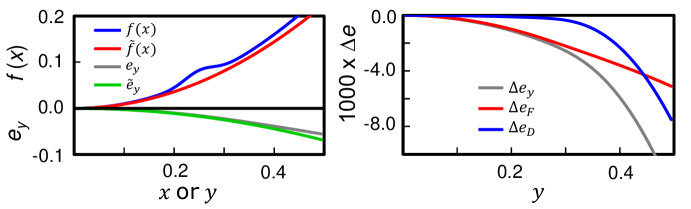
But watch what happens when we add a small Gaussian, $a\exp(-[(x-b)/c]^{2}/2)$ to $f(x)$, where $a$ is 0.02, $b$ is 0.25, and $c=0.03$. This has a relatively small effect on $\tilde{f}$, and even on $\tilde{e}_{y}$, as shown in Figure 4. However, consider the right panel in Figure 4, which shows the total error and its decomposition as a function of $y$. For $y\leq 0.3$, the system is normal, and $|\Delta e_{D}|<<|\Delta e_{y}|$. But as we approach $y=0.4$, $|\Delta e_{D}|$ grows much more rapidly than $|\Delta e_{F}|$, and even becomes larger than it after $y=0.4$.

Figure 4: (Left) Exact function and its approximation (versus $x$) above 0, and $e_{m}$ and its approximation (versus $y$) below 0. (Right) Error at minimum and its decomposition for the toy model.

How has this happened? The feature we added is not large, but it does vary rapidly. Thus $\tilde{f}\approx f$ everywhere, but $\tilde{f}^{\prime}$ is not close to $f^{\prime}$. This causes a large error in $x_{m}$ which produces a large error in $\tilde{e}(y)$, whose origin is quite different from the normal case. A careful expansion about the exact and approximate minima yields:

$$\Delta e_{D}/\Delta e_{F}=-(\Delta f^{\prime}_{m})^{2}/(f^{\prime\prime}_{m}\Delta f_{m})$$ (30)

where $\Delta f=\tilde{f}-f$. In the normal case, $\Delta f,\Delta f^{\prime},\Delta f^{\prime\prime}$ are all comparable in size so Equation 30 is small. we see that $\Delta e_{D}$ is much smaller than $\Delta e_{F}$. But if $|\Delta f^{\prime}_{m}|\geq\sqrt{f^{\prime\prime}_{m}\,|\Delta f_{m}|}$, then the calculation is abnormal, and $|\Delta e_{D}|$ dominates $|\Delta e|$. In the specific case we just calculated, we find $y=2x_{m}$, so when $x_{m}=0.1$, the center of the Gaussian, $y$ is 0.2, and the system becomes abnormal.

3.2 Extension to functionals

We can apply everything from our toy problem to the minimization of approximate functionals. The density of any approximate DFT calculation satisfies:

$$\frac{\delta\tilde{F}}{\delta n({\bf r})}\Bigg{|}_{\tilde{n}}=-v({\bf r})~{}~{}~{}{\rm or}~{}~{}~{}\tilde{n}({\bf r})=\left\{\frac{\Delta\tilde{F}}{\delta n}\right\}^{-1}[-v]({\bf r}).$$ (31)

Just as in the toy, even if $\tilde{F}\approx F$ near $n({\bf r})$, rapid changes in $F$ with $n({\bf r})$ that are not in $\tilde{F}$ can produce unusually poor densities, leading to density-driven errors. It is well-knownPPLB82 (Per+82) that total energies have derivative discontinuities at integer values of $N$ and that these are also present in the exact $F[n]$, while standard approximations that are explicit density functionals (such as TF and GGA) produce smooth functions of $N$. Thus, whenever such discontinuities are important, we should watch out for density-driven errors.

Taking another functional derivative of Equation 31 with respect to $v({\bf r})$ yields the density change in response to a perturbation:

$$\delta\tilde{n}({\bf r})=\int d^{3}r^{\prime}\,\tilde{\chi}[n]({\bf r},{\bf r}^{\prime})\,\delta v({\bf r}^{\prime})$$ (32)

where $\tilde{\chi}$ is the (static) density-density response function, and is the inverse of $\delta\tilde{F}/\delta n({\bf r})\delta n({\bf r}^{\prime})$. By analogy with Equation 30, the ratio $\Delta E_{D}/\Delta E_{F}$ is proportional to $\tilde{\chi}$. An unsually large response function suggests a significant density-driven error.

Pure DFT calculations, at least those with approximations dominated by the TF approximation, are always abnormal, i.e., the error is always density-driven. On the other hand, most modern self-consistent KS-DFT calculations have excellent densities and are normal. However, in a variety of well-known situations, the density-driven error with standard approximations (GGA and hybrids) becomes unusually large, and dominates the error in the calculation. Such errors can all be greatly reduced by using a more accurate density. Finally, in the last section, we show how PDFT errors can be understood with this analysis.

In fact, we can do a simple case exactlyB07 (Bur07). Consider same-spin non-interacting fermions in a flat box in one dimension, the simple problem usualy done first in any quantum text book. The potential energy is zero everywhere, and the total energy is all kinetic. For one particle in a box of length 1, $T=\pi^{2}/2$ exactly. On the other hand, the TF approximation for such a problem is:

$$T^{\rm TF}[n]=\frac{\pi^{2}}{6}\int dx\,n^{3}(x).$$ (33)

Minmizing in the box yields a constant density, $n=1$. Thus $T^{\rm TF}=\pi^{2}/6$, being too small by a disastrous factor of 3. However, if we insert $n(x)=\sin^{2}(x)/2$ into $T^{\rm TF}[n]$, we find a much better answer, $T^{\rm TF}[n]=5\pi^{2}/12$, i.e., we are now only too small by 1/6. Thus the TF functional is far more accurate on the exact density than the self-consistent one. In terms of our energy-error analysis, we find

$$\Delta E_{F}=\frac{1}{4}\Delta E,~{}~{}~{}~{}\Delta E_{D}=\frac{3}{4}\Delta E,$$ (34)

i.e., the density-driven error is three times larger than the functional-error. These features remain true for all values of $N$. Although TF theory becomes relatively exact here as $N\to\infty$, the density-driven error is always three times larger than the functional-error, and dominates the energy-error. This calculation is always abnormal.

4 Pure DFT

We begin with simple examples that can be easily done with Mathematica. Consider the Bohr atom, which is an atom in which the electron-electron repulsion has been turned offHL95 (HL95). The orbitals are purely hydrogenic, and the energies are those of a sum of the lowest hydrogenic levels. Solving the Euler equation yields the TF density for this problem:

$$n^{\rm TF}(r)=\frac{4Z}{\pi^{2}r^{3}_{c}}\,\left(\frac{r_{c}}{r}-1\right)^{3/2}\Theta(r_{c}-r),$$ (35)

where $r_{c}\!=\!(18/Z)^{1/3}$, and $\Theta$ is the Heaviside step function. The TF energy is just $-Z^{2}(3N/2)^{1/3}$, where $Z$ is the nuclear charge and $N$ the number of occupied orbitals. For $Z=1$, this yields a ground-state energy of $-1.144$, which is more than double the exact answer of $-1/2$. On the other hand, evaluating the TF kinetic energy on the hydrogen atom density yields:

$$E^{\rm TF}[n]=\frac{81(3\pi)^{2/3}}{1250}-1\approx-0.711,$$ (36)

which is (only) a 40% overestimate in magnitude, and the calculation is abnormal. TF errors are similar for real atoms. In radon, $\Delta E^{{}^{\rm TF}}\simeq-3400$, and the relative energy-error vanishes as $Z\rightarrow\infty$LS73 (LS73). But $\Delta E_{F}\simeq-620$, so most of the energy-error is due to the density-error. There is no reason to think that this behavior would be any different in molecular calculations, or calculations of insulating solids. It might change for simple metals with a pseudopotential, where the (pseudo)density is closer to slowly-varying.

Standard approaches to orbital-free DFT that are dominated by local and semilocal approximations are likely to have errors dominated by the density. Calculations that test kinetic energy functionals on the exact KS density rather than self-consistently will typically have much smaller errors than self-consistent calculations. Furthermore almost all semilocal approximations fail to converge in self-consistent calculations. XC15 (XC15) The focus should be on improving the functional derivative rather than the energy itself, and the measure of improvement should be the reduction of the density-driven error.

An entirely new method of finding the kinetic-energy functional has recently appeared, using machine-learning to learn from solved casesSRHM12 (Sny+12, Li+15a, Vu+15). But its functional derivatives are so poor that they are totally unusable for finding a self-consistent solution. Several techniques have been developed which constrain a minimization to stay on the manifold of densities on which the machine-learned functional is accurateSRHB13 (Sny+13a, Sny+13). These lead to algorithms that produce accurate densities, although the density-driven error is up to 10 times greater than the functional error, and the solutions also are slightly dependent on the starting point. This has led to attempts to map the density-potential functional directly, bypassing the need for an accurate functional derivativeBLBM16 (Bro+16).

5 KS-DFT

We next apply the principles of inconsistency to KS-DFT. The KS scheme is simply an elaborate way to minimize an approximation to $F$, given by Equation 8. All the same principles apply to $\tilde{E}_{\scriptscriptstyle\rm XC}[n]$ as we have already discussed about $\tilde{F}$. Because GGA and hybrids use continuous explicit density functional approximations, they miss the derivative discontinuity, which shows up in the XC functional. Thus their derivatives are highly inaccurate, as in Figure 2. The KS potential of these approximations is too shallow by several eV, yielding poor orbital energies, but the potentials are almost perfect constant shifts relative to the exact potentials, at least within most of the atom or molecule. Such a shift has no effect on the shape of the orbitals, and therefore on the density. In fact, most KS-DFT calculations have excellent densities so even for cases with poor results, their errors are functional-driven, not density-drivenTS66 (TS66). For the He atom of Figure 2, $\Delta E_{D}$ is -9% of $\Delta E$ in PBE. The functional error dominates and the error in PBE worsens if the exact density is used. Thus, all KS-DFT calculations with the standard functionals have poor-looking KS potentials. In a certain subset of cases, these poor quality potentials will lead to sufficiently poor self-consistent densities that density-driven errors become significant. Such calculations are abnormal and, if a more accurate density is available, the error reduces significantly.

Is there any way to know, a priori, if a given approximate DFT calculation is likely to suffer from a density-driven error? There is. The KS response function is

$$\tilde{\chi}_{\scriptscriptstyle\rm S}({\bf r},{\bf r}^{\prime})=\sum_{i,j}(f_{i}-f_{j})\frac{\tilde{\phi}_{i}^{*}({\bf r})\tilde{\phi}_{j}^{*}({\bf r})\tilde{\phi}_{i}({\bf r}^{\prime})\tilde{\phi}_{j}({\bf r}^{\prime})}{\tilde{\epsilon}_{i}-\tilde{\epsilon}_{j}+i0_{+}}~{},$$ (37)

where $f_{i}$ is the KS orbital occupation factorDG90 (DG90). The smallest denominator is $\Delta\tilde{\epsilon}_{g}$, the HOMO-LUMO gap. Normally, the difference between the exact and approximate $v_{\scriptscriptstyle\rm S}({\bf r})$ is small, ignoring any constant shift. If $\Delta\tilde{\epsilon}_{g}$ is not unusually small, this error leads to a small error in $\tilde{n}({\bf r})$. But if $\Delta\tilde{\epsilon}_{g}$ is small, even a small error in $v_{\scriptscriptstyle\rm S}({\bf r})$ can produce a large change in the density, and self-consistency only increases this effect. Thus small $\Delta\tilde{\epsilon}_{g}$ suggests a large density-error, and the calculation should be checked. This is done by inserting an accurate density in the approximate functional. If the energy changes significantly, the energy should be substantially more accurate on the exact density.

Figure 5: ExactUG94 (UG94) and approximate densities and KS potentials of H^-. The dashed horizontal lines are eigenvalues of 1s orbital with PBE and EXX in a.u..

To illustrate this effect in its strongest form, we calculate the energy of H^-. This anion has two electrons, just like He, but it is long knownSRZ77 (SRZ77) that a standard DFT calculation, in the infinite basis-set limit, cannot bind two electrons. In fact, a fraction of an electron is lost to the continuum. To fully converge such a calculation, we set the occupation of the 1s orbital to, e.g., 1.5, and find a converged solution. We then slowly increase the occupation until the HOMO level hits exactly zero. This is then the lowest-energy self-consistent PBE solution. Its density is very poor (see Figure 5) as it is missing 0.37 electrons. The error in its energy is the same magnitude as of He (see Table I), but now it is too negative. On the other hand, the HF density binds 2 electrons with a negative HOMO, but its energy is very poor. Finally, the green curve in Figure 5 is the PBE potential on the QMC density. It has a positive HOMO (really a resonance) and, in a limited basis set, will yield an accurate self-consistent density (but is not converged).

Of course, the value of DFT is in its computational speed, and would be lost if we had to calculate a highly accurate density by some other method every time we ran into a density-driven error. But because extreme density-driven errors are due to the lack of derivative discontinuity in the energy, which is reflected in the XC potential, a HF density from an orbital-dependent functional, does not suffer from such errors, and is exact for one electron. Thus the HF density is better for such systems, as we show below. So we name the method HF-DFT, meaning to use a HF density with DFT energies. From Table 1, we see that, evaluating PBE on the QMC density of H^-, yields an incredibly accurate answer. HF-DFT also substantially improves over self-consistent DFT but, because this case is so severe, further improvement is gained from the QMC density.

Technically, it is not so easy to precisely perform a KS calculation on a HF density, as one must find the KS potential by a process of inversion, which can be complicated and difficult to converge. A simple workaround is to approximate the HF-DFT energy as

$$E^{\rm HF-DFT}\approx E^{\rm HF}+(\tilde{E}_{\scriptscriptstyle\rm XC}[n^{\rm HF}]-E_{\scriptscriptstyle\rm X}^{\rm HF}).$$ (38)

Because of the variational principle, this is accurate to second-order in the density difference, which turns out to be good enough. On a website one can find instructions that perform this procedure for several standard codes. The basic trick is to take the output density of a converged HF calculation, and feed it into a DFT cycyle, but set the number of iterations to zero or one depending on the code.

5.1 History of HF-DFT

The use of HF densities in DFT calculations has a long history. Even before the mid 90’s, it was common practice to test approximate density functionals on HF densitiesB88 (Bec88, SSP86). When DFT was first becoming popular for routine calculations on main group elements, the initial calculations were performed on HF densities, in order to compare “apples-to-apples”GJPF92 (Gil+92, OB94). Pioneering work even noted that, in difficult cases, HF densities somehow yielded better results than self-consistent resultsS92 (Sad92). More recently, the improvement in barrier heights of transition states has been repeatedly observeredJS08 (JS08, VPB12).

But what was previously missing was a general explanation for these better results, and a way to predict when HF-DFT would be better than self-consistent DFT. In fact, for normal systems, HF-DFT is often slightly worse, as we saw for the He atom, and in many ways, the HF density is less accurate than the self-consistent DFT densityGMB16 (GMB16). Moreover, the theory given in Section 5 is entirely general, applying to any approximate DFT calculation, not just those with semilocal functionals. Thus our method explains how and when HF-DFT is a useful idea.

5.2 Electron affinities

The origin of the current theory lies in the calculation of electron affinities with DFT. For many years, the Schaefer group successfully calculated electron affinities within DFTRTS02 (RK+02). By using the same basis for both the anion and the neutral species, finding the DFT energy difference, and increasing the basis set until the answer stopped changing. This worked in many cases, especially those of biological interestDS09 (DLS09, GXS10, GXS10a, Che+10, KS10). A slight flaw was that the HOMO of the anion would be positive (see Figure 5), which meant these calculations were unconvergedRT97 (RT97).

The answer to this apparent conundrum is given by the green curve of Figure 5. Although the HOMO is technically a resonance, the width of the barrier holding the electron in is so wide that any standard basis functions will not detect the lower-energy state outside the barrier. Hence the reasonable performance and apparent convergence of electron affinities. However, the truly converged result is the one mising a fraction of an electron, which has a terrible energy(Table 1).

But this also suggested an alternative, more satisfying approach. Since the problem is with the self-consistency of the density, if a more accurate density was available (in this case, a bound one), it should also work. Thus HF-DFT was used, and found to give comparable (or better) results for atoms and small molecules. In fact, using this method, electron affinities are typically twice as good as ionization potentials with approximate DFTLB10 (LB10, LFB10). It should be used for all anionic DFT calculations in future. It was quite surprising that no-one seemed to have applied this logic to the anion problem in DFT before.

The explanations in the papers addressing electron affinities are given in the language of self-interaction errorLB10 (LB10, LFB10, KSB11). This was later generalized to the general energy-error analysis discussed here, when it was discovered that DFT calculations on radicals can also be improved with HF-DFT, even though no species are chargedKSB13 (KSB13, KSB14).

We use HF densities because they are computationally accesible for molecular systems. We should use the exact density, but often HF densities are sufficiently good that any remaining density-driven error is much smaller than the functional-error. But HF densities are not always good enough, or even a good choice. For example, for H^-, the HF-PBE energy is -0.521 Hartree, which is substantially different from the QMC-PBE energy(-0.527 Hartree). Another typical failing is when the HF calculation suffers from substantial spin contamination. Then the HF density is certainly not accurate enough, and a more advanced method must be used. Finally, we mention that for solids, especially metals, HF calculations can be very expensive and problematic, so in this case, some other method would be better for calculating an accurate density (for an abnormal system).

Affinities involved in the successive fluorination of ethylene are afflicted by positive HOMO’s and the standard basis set treatment failsPDT10 (PDPT10). For the most extreme example, see also Refs MUMG14 (Mir+14, GB15). Using a reasonable basis set is often used to coax an electron affinity from a standard functional when evaluating on a data base involving anionsCPR10 (CPR10, Hao+13). Many authors emphasize the importance of the basis for DFT calculations of electron affinityCHKK15 (Cho+15, Coo+15), and some have explored the difficulties in extracting electron affinitiesTDGT14 (Tea+14). The relation between derivative discontinuities, delocalization error and positive HOMO values is extensively explored in Ref. PTHT15 (Pea+15). The importance of exact exchange has also been noticed for genuinely meta-stable anionsFDAB14 (Fal+14), where the HOMO is positive.

5.3 Binding curves

Our next abnormality is a well-known failing of standard DFT approximationsRPC06 (Ruz+06). KS-DFT calculations of molecular dissociation energies ($E_{b}$) are usefully accurate with GGA’s, and more so with hybrid functionals. These errors are often about 0.1 eV/bondES99 (ES99), but are found by subtracting the calculated molecular energy at its minimum from the sum of calculated atomic energies.

However, things look very different if one calculates a binding energy curve by simply plotting the molecular energy as a function of atomic separation $R$. This is because, if one simply increases the bond lengths to very large values, the fragments fail to dissociate into neutral atoms. Incorrect dissociation occurs whenever the approximate HOMO of one atom is below the LUMO of the otherRPC06 (Ruz+06), which guarantees a vanishing $\Delta\tilde{\epsilon}_{g}$ when the bond is greatly stretched. With standard functionals, this happens for more than half of all heteronuclear diatomic pairs. The exact $v_{\scriptscriptstyle\rm XC}({\bf r})$ contains a step between the atoms which is missed by standard approximations. Since the step is often dominated by the exchange term, effectively only a fraction of this step is contained in a hybrid calculation. In the very stretched case, this effect can also be explained in terms of the inability of the approximations to reproduce the derivative discontinuity in the energy.

Figure 6: Binding energy curves of CH⁺ with various methods. The cross mark is MRCI results from Ref. BSM14 (BSM14). Energies are in eV.

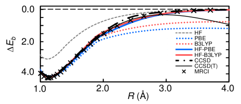
A recent paperKPSS15 (Kim+15) describes how to perform HF-DFT calculations that both overcome the dissociation limit problem, and yield accurate binding energy curves out to much larger separations than was previously possible. A beautiful example is posed by a molecule that is very challenging to theory, CH⁺ (but of perhaps limited interest experimentally). All DFT methods perform satisfactorily near the bond minimum, yielding accurate atomization energies when subtracted from the corresponding atomic calculations of C⁺ and H. They can be compared with the ‘gold standard’ of ab initio quantum chemistry, CCSD(T). However, as the bond is stretched, it becomes multi-reference in character, and even CCSD(T) fails badly. The perturbative treatment of triple excitations fails as the gap shrinks to zero. CCSD behaves better, but only a multi-reference configuration interaction (MRCI) calculation yields an accurate curve. Self-consistent DFT yields incorrect dissociation limits and, even worse, deviates from the accurate curve at only 2 Å. However, Figure 6 shows HF-DFT works extremely well here, closely following the accurate curve out much further, as well as producing the correct dissociation products, for most approximate functionals.

5.4 Potential energy surfaces of radical and charged complexes

There are many branches of chemistry in which either radicals or anions, dissolved in water, are vitally important. To perform ab initio molecular dynamics simulations of such systems, KS-DFT calculations must yield accurate potential energy surfaces for the complexes. DFT calculations with standard functionals often yield incorrect global minima with fictious hemi-bonds appearing, in which the additional electron localizes halfway between two species. This is blamed on self-interaction error. HF-DFT cures all these problems, making potential energy surfaces highly accurate with any of the popular functionalsKSB14 (KSB14).

5.5 Applications of energy-error analysis and other approaches

There are already many applications in the literature where the energy-error analysis has been applied to calculations with abnormal standard approximations. As the length of a long-chain hydrocarbon grows, the ionization potential collapses to the KS HOMO level with standard approximations, due to the incorrect delocalization of the hole over the entire moleculeWVIJ15 (Whi+15). This effect should not be present in HF-DFT, but that has yet to be tested. Gaps have been analyzed to see if a strong density-driven error is responsible for poor performance for RNA backbonesKMGH15 (Kru+15). The energy-error analysis has also been used in analyzing errors in 3-body DFT energiesG14 (Gil14). The delocalization error has been implicated in difficulties calculating alkylcobalaminsGNPM13 (Gov+13), where HF-DFT might be very helpful. It has also been useful in analyzing intercage electron transfer in Robin-Day type moleculesWLZL12 (Wan+12), and a large density-driven error has been found in the Kevan model of a solvated electronJOD13 (JRD13). IR spectra of small anionic water clusters have been shown to be problematic with fixed basis DFT calculations, and fixed by MP2GDTJ15 (Gon+15). But HF-DFT has not been tried, and should be better than MP2.

There are also cases where HF-DFT has definitely improved results. HF-DFT has been used (successfully) to deal with anion, dianion, and radical Fullerene oligomersSSSZ14 (Shu+14). In diene isomerization, the energy-error analysis has been performed, with a strong suggestion that inconsistency improves energeticsWPAS15 (Wyk+15). Magnetic exchange couplings can be greatly improved by inconsistent calculationsPP12 (PP12), and might also be relevant to organic moleculesKCL13 (KCL13). It is useful even in estimating metabolic reaction energiesJRDS14 (Jin+14).

Not all suspected density-driven errors turn out to be so, and in those cases, HF-DFT does not work. For adhesive energies of hydrogen molecular chains, HF-DFT only slightly improves over DFTSX15 (SX15), presumably because this is not a density-driven error, as all units in the chain are identical just as in Figure 1. We have explored HF-DFT as a cure for self-interaction error in anion-$\pi$ complexesMCRS15 (Mez+15), but found it not to be density-driven.

There are countless other approaches to fixing the problems of abnormal calculations in the DFT literature. Range-separated functionals have been shown to cure delocalization errors of standard functionals in Michael-type reactionsSAR13 (SAR13), but HF-DFT should also work, while bypassing the need to introduce a system-dependent parameter. Other authors have suggested constraining the potentials of DFT calculations with the correct asymptotic formsGL12 (GL12), which is another approach ripe for energy-error analysis. Other alternatives include using Koopman’s conditionDFPP13 (Dab+13), or the use of a model for the exchange hole that avoids the delocalization effect on barrier heightsJCDD15 (Joh+15). The beauty of HF-DFT is that it bypasses the need to find a better potential or do a more expensive calculation. It is possibly the most pragmatic approach to these difficulties, and readily available to any user.

Of course, more sophisticated (and usually more expensive) calculations such as RPA usually do not suffer from the specific errors made by standard approximationsEBF12 (EBF12). But many such methods suffer from acute orbital-dependence: significantly different energies are found by using different non-self-consistent orbitals, and self-consistent calculations are often hideously expensive, both in terms of computational time and coding, without providing improved results. These situations are ripe for energy-error analysis.

In fact, many applications of hybrid functionals face a Procrustean dilemma. The small value of $a$ is needed to yield accurate energeticsBb93 (Bec93a, PEB96), but a value closer to 100% is needed to generate accurate potentials and response properties (as in Figure 2). The use of a local hybridBCL98 (BCL98) should overcome the dilemma posed by global hybrids in this regardJ14 (Joh14). Abnormal systems make this problem acute. But HF-DFT sidesteps the issue, by using a better density without studying the potential. An ensemble generalization is one of many other approaches to this problemKSKK15 (Kra+15).

5.6 Limitations of HF-DFT

The classic examplesMCY08 (MSCY08) of failures of popular DFT approximations are the binding energy curves of H₂ and H${}_{2}^{+}$. These two prototypes illustrate starkly the failures as bonds are stretched, and these effects happen for most bonds. Unfortunately, HF-DFT does not help here, because of the left-right symmetry in both cases. Both these errors are functional-driven, i.e., replacing the self-consistent density with the exact density makes little difference. In Figure 1), the dashed lines are on the exact (HF) density, and are very similar to the self-consistent solid lines.

Figure 7: Decomposition of the partition energy-error $\Delta E_{p}$ (left) and total fragment energy-error $\Delta E_{\rm frag}$ (right) for PBE (blue) and OA (red). Dotted curves functional-driven, dashed density-driven. Energies are in eV.

6 PDFT and energy-error analysis

6.1 Interpretation of PDFT energies

Separating functional and density-driven errors can also illuminate the results of embedding calculations GBMM12 (Goo+12) and clarify the role of self-consistency in S-DFT calculations WS13 (WS13). Now we apply the energy-error analysis to a PDFT calculation in which we know the exact XC functional, but approximate $\tilde{E}_{p}=0$. Then we trivially find our energy as the sum of isolated fragments with corresponding fragment densities. Our energy-error is simply

$$\Delta E=E_{\rm frag}^{(\infty)}-E=-E_{\rm dis},~{}~{}\Delta E_{F}=-E_{p},~{}~{}\Delta E_{D}=E_{\rm rel},$$ (39)

i.e., we can interpret the partition energy as (minus) the functional error of such a calculation, and the relaxation energy as the density-driven error. We then say that bonds are normal when $|E_{\rm rel}|<<|E_{\rm dis}|$. Abnormal bonds are those in which the distortion of the fragment densities relative to the corresponding atomic densities is sufficiently large to make the relaxation energy comparable to the dissociation energy. This definition is precise and unambiguous, and does not depend on any XC approximation.

6.2 Energy-error analysis within PDFT

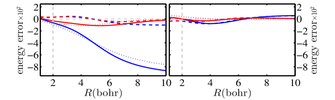
As our last example, we apply the energy-error analysis within an approximate PDFT calculation. We use the OA of Equation 25 on PBENW15 (NW15). We write

$$\Delta E_{p}=\Delta E_{p,F}+\Delta E_{p,D},~{}~{}~{}\Delta E_{\rm frag}=\Delta E_{{\rm frag},F}+\Delta E_{{\rm frag},D}$$ (40)

We plot these in Figure 7. The blue in the left panel of Figure 7 shows that the large error in $E_{p}$ is functional driven, as expected. Even when largely fixed by the overlap approximation, for moderate bond lengths, this is still functional driven. But for $R>5$, the density-driven error comes to dominate even the OA result, suggesting it can be improved by using the HF density (just as the heteronuclear bonds of Section 5.3). On the other hand, the fragment errors of the right panel of Figure 7 are much smaller overall. Moreover, for $R>4$, these errors are density-driven and so can be reduced with HF-DFT. For $R<4$, the density-driven component remains comparable to the functional-driven piece, which is the same for both PBE and OA. This strongly suggests that, at least for H${}_{2}^{+}$, HF-DFT can reduce the fragment errors, once the principal partition energy-error has been tackled within PDFT.

7 Conclusion

Emersonemerson (Eme47) was clearly referring to DFT and PDFT when he wrote that a foolish consistency is the hobgoblin of little minds. Previously, anyone questioning whether DFT calculations should be self-consistent would be regarded as showing signs of triviality. We hope to have convinced the readers, possibly for the first time in their lives, of the vital Importance of Being Consistent (when not foolish).