High-Dimensional Bayesian Regularized Regression with the bayesreg Package

Abstract

Bayesian penalized regression techniques, such as the Bayesian lasso and the Bayesian horseshoe estimator, have recently received a significant amount of attention in the statistics literature. However, software implementing state-of-the-art Bayesian penalized regression, outside of general purpose Markov chain Monte Carlo platforms such as Stan, is relatively rare. This paper introduces bayesreg, a new toolbox for fitting Bayesian penalized regression models with continuous shrinkage prior densities. The toolbox features Bayesian linear regression with Gaussian or heavy-tailed error models and Bayesian logistic regression with ridge, lasso, horseshoe and horseshoe$+$ estimators. The toolbox is free, open-source and available for use with the MATLAB and R numerical platforms.

1 Introduction

Bayesian penalized regression techniques for analysis of high-dimensional data have received a significant amount of attention in the statistics literature. Recent examples include the Bayesian lasso [Park and Casella, 2008, Hans, 2009], the normal-gamma estimator [Griffin and Brown, 2010], the horseshoe and horseshoe$+$ estimators [Carvalho et al., 2010], and the generalized double Pareto estimator [Armagan et al., 2013], among others. These estimators use sparsity inducing prior distributions for the regression parameters and are commonly applied in the setting of big data, where most of the predictor variables are assumed to be unassociated with the outcome. Sparsity inducing priors are implemented with exchangeable Gaussian variance mixture distributions, and the corresponding Bayesian posterior inferences often directly correspond to well-known penalized regression techniques, such as the lasso [Tibshirani, 1996, 2011] and the elastic net [Zou and Hastie, 2005]. For a comprehensive catalog of Bayesian penalized regression techniques and their frequentist analogues, see [Polson and Scott, 2010, 2012].

There are many software tools for fitting standard penalized regression estimators, with glmnet [Friedman et al., 2010] and ncvreg [Breheny and Huang, 2011] being the two most popular implementations in practice. The software toolbox glmnet implements the lasso and elastic net penalty for generalized linear models, while ncvreg provides an efficient algorithm for fitting MCP [Zhang, 2010] or SCAD [Fan and Li, 2001] regularization paths in linear and logistic regression models. Both of these implementations are freely available open-source packages for the R statistical platform. In contrast, software for Bayesian penalized regression, outside of general purpose Markov chain Monte Carlo (MCMC) platforms such as WinBUGS and Stan, is scarce (see Section 4). Given the excellent theoretical properties of Bayesian penalized regression methods, it would be of great benefit to the research community if a software toolbox implementing these approaches was made available. To this end, the main contribution of this manuscript is a software toolbox that implements state-of-the-art Bayesian penalized regression estimators for linear and logistic regression models. This toolbox is free, open-source and features significant computational advantages over existing toolboxes. Further, the toolbox is implemented for both the MATLAB and the R numerical computing platforms.

A technical description of the Bayesian regression toolbox is now given. Formally, consider the following Bayesian regression model for data ${\bf y}=(y_{1},\ldots,y_{n})^{\mathrm{\scriptscriptstyle T}}\in\mathbb{R}^{n}$ given a matrix ${\bf X}=({\bf x}_{1},\ldots,{\bf x}_{n})^{\mathrm{\scriptscriptstyle T}}\in\mathbb{R}^{n\times p}$ of $p$ predictor variables:

$$z_{i}|{\bf x}_{i},\bm{\beta},\beta_{0},\omega_{i}^{2},\sigma^{2} \sim \mathcal{N}_{n}({\bf x}_{i}^{\mathrm{\scriptscriptstyle T}}\bm{\beta}+\beta_{0},\sigma^{2}\omega_{i}^{2}),$$ (1)

$$\sigma^{2} \sim \pi(\sigma^{2})\,d\sigma^{2},$$ (2)

$$\omega_{i}^{2} \sim \pi(\omega_{i}^{2})\,d\omega_{i}^{2},$$ (3)

$$\beta_{0} \sim d\beta_{0},$$ (4)

$$\beta_{j}|\lambda_{j}^{2},\tau^{2},\sigma^{2} \sim \mathcal{N}(0,\lambda_{j}^{2}\tau^{2}\sigma^{2}),$$ (5)

$$\lambda^{2}_{j} \sim \pi(\lambda^{2}_{j})\,d\lambda^{2}_{j},$$ (6)

$$\tau^{2} \sim \pi(\tau^{2})\,d\tau^{2},$$ (7)

where $i=(1,\ldots,n)$, $j=(1,\ldots,p)$, $\beta_{0}\in\mathbb{R}$ is the intercept parameter, $\bm{\beta}\in\mathbb{R}^{p}$ are the regression coefficients, and the variables $(z_{1},\ldots,z_{n})$ are set appropriately depending on whether the data ${\bf y}$ is continuous (see Section 2.1) or binary (see Section 2.2). In big data problems, the sample size $n$ is often less than the number of predictors (i.e., $p\gg n$), and the predictor matrix ${\bf X}$ is not full rank.

The hierarchy (1)–(7) consists of two key groups: (i) the model for the sampling distribution of the data (1)–(3) and (ii) the prior distributions for the regression coefficients (5)–(7). Statistical models for both the data and the prior distributions are constructed from exchangeable Gaussian variance mixture distributions [Andrews and Mallows, 1974]. The probability density function of a Gaussian scale mixture random variable $Z$ can be written as

$$\pi_{Z}(z|\mu,\sigma^{2})=\int_{0}^{\infty}{\rm N}(z|\mu,g(\lambda)\sigma^{2})\pi_{\lambda}(\lambda)\;d\lambda,$$ (8)

where $N(\cdot|\mu,\sigma^{2})$ denotes the Gaussian distribution with mean $\mu\in\mathbb{R}$ and variance $\sigma^{2}>0$, $g(\lambda)$ is a positive function of the mixing parameter $\lambda$, and $\pi_{\lambda}(\cdot)$ is a mixing density defined on $\mathbb{R}^{+}$. Particular choices of the mixing parameter $\lambda$ and the mixing density $g(\lambda)$ can be used to model a wide variety of non-Gaussian distributions. For example, selecting the gamma distribution ${\rm Ga}(\delta/2,\delta/2)$ as the mixing density and setting $g(\lambda)=1/\lambda$ yields the Student $t$ density with $\delta>0$ degrees of freedom. This decomposition may alternatively be written in the following hierarchical form:

$$Z|\mu,\sigma^{2},\lambda\sim{\rm N}(\mu,\sigma^{2}/\lambda),\quad\quad\lambda|\delta\sim{\rm Ga}(\delta/2,\delta/2).$$ (9)

There are many distributions that admit the scale mixture of Gaussians representation; for example, the logistic density [Polson et al., 2013], the Laplace distribution [Andrews and Mallows, 1974], and the class of $z$ distributions [Barndorff-Nielsen et al., 1982].

In the case of the data model (1)–(3), the scale parameter $(\sigma^{2}>0)$ and the latent variables $(\omega_{1},\ldots,\omega_{n})$ are used in a Gaussian scale mixture framework to represent a variety of common regression models for both binary and continuous data. In particular, we consider Gaussian linear regression (see Section 2.1), linear regression with Laplace errors (see Section 2.1.2), linear regression with Student $t$ errors (see Section 2.1.3), and binary logistic regression (see Section 2.2). The hyperparameters $(\tau^{2}>0)$ and $(\lambda_{1},\ldots,\lambda_{n})$ will be used to model different sparsity inducing prior distributions for the regression coefficients. The prior distributions considered in this paper are examples of common global–local shrinkage priors and include: the lasso (see Section 2.3.2), ridge regression (see Section 2.3.1), the horseshoe (see Section 2.3.3), and the horseshoe$+$ estimator (see Section 2.3.4). Details of the software toolbox implementing these Bayesian penalized regression techniques are given in Section 3.

2 Bayesian penalized regression

Bayesian inference for a statistical model requires the posterior distributions for all model parameters. In the case of the penalized regression hierarchy (1)–(7), analytical computation of the posterior distributions is intractable and we instead use MCMC techniques to obtain stochastic approximations to the corresponding posterior densities. Due to the particular choices of the prior distributions (see Section 2.3), all conditional posterior distributions are computable analytically, and sampling from these posterior densities can be done with the Gibbs sampler [Geman and Geman, 1984].

We use the uniform prior distribution for the intercept parameter (4) while the regression parameters are given a joint prior distribution specified by the Gaussian variance mixture (5)–(7). Given the aforementioned choice of prior distributions, the conditional posterior distributions for the intercept parameter $\beta_{0}$ and the regression parameters $\bm{\beta}$ are equivalent across the statistical models examined in this paper. Let

$$e_{i} = z_{i}-{\bf x}_{i}^{\mathrm{\scriptscriptstyle T}}\bm{\beta}-\beta_{0},\quad(i=1,\ldots,n),$$ (10)

$$\bm{\Omega}_{n} = \sigma^{2}\,{\rm diag}(\omega_{1}^{2},\ldots,\omega_{n}^{2}),$$ (11)

$$\bm{\Lambda}_{p} = \sigma^{2}\tau^{2}\,{\rm diag}(\lambda_{1}^{2},\ldots,\lambda_{p}^{2}),$$ (12)

where $(e_{1},\ldots,e_{n})$ denote the model residuals in the case of linear regression and $\bm{\Omega}_{n}\in\mathbb{R}^{n\times n}$ and $\bm{\Lambda}_{p}\in\mathbb{R}^{p\times p}$ are diagonal matrices. In the case of linear regression models (see Section 2.1), the data $y_{i}$ is continuous and we set $z_{i}=y_{i}$, while in binary logistic regression (see Section 2.2)

$$z_{i}=\omega_{i}^{2}\left(y_{i}-\frac{1}{2}\right)$$ (13)

for all $i=1,\ldots,n$. In both cases, the conditional posterior distribution for the intercept parameter $\beta_{0}$ is the Gaussian distribution ${\rm N}(\tilde{\mu},\tilde{\sigma}^{2})$, where

$$\tilde{\mu}=\left(\sum_{i=1}^{n}\frac{z_{i}-{\bf x}_{i}^{\mathrm{\scriptscriptstyle T}}\bm{\beta}}{\omega^{2}_{i}}\right)\left(\sum_{i=1}^{n}\frac{1}{\omega^{2}_{i}}\right)^{-1},\quad\tilde{\sigma}^{2}=\sigma^{2}\left(\sum_{i=1}^{n}\frac{1}{\omega^{2}_{i}}\right)^{-1}.$$ (14)

The conditional posterior density for the regression parameters $\bm{\beta}$ is the $p$-variate Gaussian distribution ${\rm N}_{p}(\tilde{\bm{\mu}},{\bf A}_{p}^{-1})$, for which

$$\tilde{\bm{\mu}}={\bf A}_{p}^{-1}{\bf X}^{\mathrm{\scriptscriptstyle T}}\bm{\Omega}_{n}^{-1}({\bf z}-\beta_{0}{\bf 1}_{n}),\quad{\bf A}_{p}=\left({\bf X}^{\mathrm{\scriptscriptstyle T}}\bm{\Omega}_{n}^{-1}{\bf X}+\bm{\Lambda}_{p}^{-1}\right),$$ (15)

where ${\bf 1}_{n}$ is an $n$-dimensional vector of ones and ${\bf A}_{p}\in\mathbb{R}^{p\times p}$ is a symmetric positive definite precision matrix. A detailed derivation of this conditional distribution is available in the seminal paper by Lindley and Smith [1972].

In terms of computational efficiency, a major bottleneck of the proposed Gibbs algorithm is the sampling of the regression coefficients from the $p$-variate Gaussian distribution ${\rm N}_{p}(\tilde{\bm{\mu}},{\bf A}_{p}^{-1})$ when the number of predictors $p$ is large. Direct computation of the matrix inverse ${\bf A}_{p}^{-1}$ is not recommended because it exhibits poor numerical accuracy and is computationally expensive. Instead, our implementation uses two algorithms for sampling the regression coefficients, where the choice of algorithm depends on the sample size $n$ and the number of regressors $p$. Specifically, we use the algorithm in  Rue [2001] when the ratio $(p/n<2)$ and  Bhattacharya et al. [2016] otherwise.

Rue’s algorithm uses Cholesky factorization of the conditional posterior variance matrix ${\bf A}_{p}^{-1}$ and has computational complexity of the order $O(p^{3})$. The algorithm is efficient as long as $p$ is not too large compared with $n$. In the case where $p$ is much larger than $n$, our sampler uses the algorithm in Bhattacharya et al. [2016] which has computational complexity $O(n^{2}p)$, which is linear in $p$. Bhattacharya et al. [2016] show that their algorithm is orders of magnitude more efficient than Rue’s algorithm when $(p/n>2)$. Subsequently, sampling of the regression coefficients in the proposed toolbox is significantly faster than alternative implementations (e.g., Stan) and represents the current state-of-the-art in terms of speed and numerical accuracy.

In the following sections, we describe the Gaussian scale mixture framework for the data (1)–(3) for linear (Section 2.1) and logistic (2.2) regression models.

2.1 Linear regression

The Bayesian penalized regression hierarchy (1)–(7) is easily adapted to the setting of Bayesian linear regression models with Gaussian noise. In the case of contaminated data or data with outliers, the Gaussian noise model is no longer appropriate and error distributions with heavier tails are required. The decision to model the data generating distribution as the Gaussian scale mixture (1)–(3) with mixing parameters $(\omega^{2}_{1},\ldots,\omega^{2}_{n})$ allows for a wide range of non-Gaussian, heavy-tailed noise models to be easily incorporated into the main hierarchy. In particular, we implement Laplace and Student $t$ noise models, which correspond to Gaussian scale mixtures with exponential and inverse gamma mixing densities, respectively.

The model for the noise is obtained from the prior distributions for the scale parameter $\sigma^{2}$ and the latent variables $(\omega^{2}_{1},\ldots,\omega^{2}_{n})$. Recall that the data ${\bf y}$ is continuous in the case of linear regression and we set $(z_{i}=y_{i})$ in (1) and (10). The treatment for binary data in the case of logistic regression is described in Section 2.2. For all noise models considered, the scale parameter $\sigma^{2}$ is given the scale invariant prior distribution $\pi(\sigma^{2})\propto 1/\sigma^{2}$. The conditional posterior distribution for $\sigma^{2}$ is the inverse gamma distribution ${\rm IG}(\tilde{\alpha},\tilde{\beta})$, where

$$\tilde{\alpha}=\frac{n+p}{2},\quad\tilde{\beta}=\frac{1}{2}\left(\sum_{i=1}^{n}\frac{e_{i}^{2}}{\omega_{i}^{2}}+\sum_{j=1}^{p}\frac{\beta_{j}^{2}}{\tau^{2}\lambda_{j}^{2}}\right).$$ (16)

Sampling of the latent variables $(\omega^{2}_{1},\ldots,\omega^{2}_{n})$ for Gaussian, Laplace and Student $t$ noise models is described in the following sections.

2.1.1 Gaussian errors

In the case of Gaussian errors, the data is assumed to be generated by a single Gaussian distribution, not a Gaussian scale mixture distribution. The latent variables $(\omega^{2}_{1},\ldots,\omega^{2}_{n})$ are therefore set to $\omega^{2}_{i}=1$ for all $i=(1,\ldots,n)$ requiring no sampling, which implies that $\bm{\Omega}_{n}=\sigma^{2}{\bf I}_{n}$ in (11).

2.1.2 Laplace errors

The Laplace distribution has heavier tails than the Gaussian distribution and is commonly used to model contaminated data and data with outliers. An important advantage of the Laplace distribution, over other heavy-tailed distributions such as the Student $t$, is that all of its central moments are finite. We represent the Laplace distribution as a Gaussian variance mixture distribution where the mixing density (8) is

$$\omega_{i}^{2}\sim{\rm Exp}(1),$$ (17)

which is an exponential distribution with a mean of one. This particular choice of the mixing distribution ensures that the residuals $(e_{1},\ldots,e_{n})$ follow a Laplace distribution and that the scale parameter $\sigma^{2}$ (see (2)) is equal to the variance of the residuals, as in linear regression with Gaussian noise. The conditional posterior distribution of the latent variables $1/\omega_{i}^{2}$ is the inverse Gaussian distribution ${\rm IGauss}(\tilde{\mu}_{i},\tilde{\lambda})$, where

$$\tilde{\mu}_{i}=\left(\frac{2\sigma^{2}}{e_{i}^{2}}\right)^{\frac{1}{2}},\quad\tilde{\lambda}=2.$$ (18)

for all $i=(1,\ldots,n)$.

2.1.3 Student $t$ errors

An alternative to the Laplace distribution commonly used in linear regression with contaminated data is the Student $t$ distribution. The Student $t$ distribution has heavier tails than the Gaussian distribution and is parameterized by a location, a scale and a degrees of freedom parameter $(\delta>0$) that determines the heaviness of the tails. When the degrees of freedom parameter $(\delta=1)$, the Student $t$ distribution reduces to the Cauchy distribution, which has heavier tails than both the Gaussian and Laplace distributions. In addition, the Student $t$ distribution has heavier tails than the Laplace distribution for all $(\delta\leq 5)$, but, unlike the Laplace distribution, the Student $t$ distribution has infinite variance when $(\delta\leq 2)$.

From (9), the Student $t$ distribution may be written as a Gaussian variance mixture distribution where the mixing density is the inverse gamma distribution

$$\omega_{i}^{2}\sim{\rm IG}\left(\frac{\delta}{2},\frac{\delta}{2}\right),\quad(i=1,\ldots,n).$$ (19)

The choice of this inverse gamma distribution as the prior distribution of the latent variables $(\omega_{1},\ldots,\omega_{n})$ ensures that the residuals follow a Student $t$ distribution with $\delta$ degrees of freedom and that the variance of the residuals $(e_{1},\ldots,e_{n})$ is related to the scale parameter $\sigma^{2}$ (see (2)) by

$${\rm Var}(e_{i})=\sigma^{2}\left(\frac{\delta}{\delta-2}\right),\quad(i=1,\ldots,n)$$ (20)

which is finite for all $(\delta>2)$. Given the scale parameter $\sigma^{2}$ and the residuals $(e_{1},\ldots,e_{n})$, the conditional posterior distribution for the latent variables $\omega_{i}^{2}$ is the inverse gamma distribution ${\rm IG}(\tilde{\alpha},\tilde{\beta}_{i})$ where

$$\tilde{\alpha}=\frac{\delta+1}{2},\quad\tilde{\beta}_{i}=\frac{1}{2}\left(\frac{e_{i}^{2}}{\sigma^{2}}+\delta\right).$$ (21)

2.2 Binary logistic regression

In the case of binary data $y_{i}\in\{0,1\}$ $(i=1,\ldots,n)$, the relationship between the predictor variables and the outcome variable is represented using binary logistic regression models. In particular, we assume that

$$p(y_{i}=1|{\bf x}_{i},\beta_{0},\bm{\beta})=\frac{1}{1+\exp\left(-(\beta_{0}+{\bf x}_{i}^{\mathrm{\scriptscriptstyle T}}\bm{\beta})\right)}.$$ (22)

Direct sampling from the posterior distribution of the regression parameters in this binary logistic regression model is difficult due to the mathematical form of the logistic function. Recently, indirect sampling algorithms based on auxiliary (or latent) variables for logistic regression have been proposed by Holmes and Held [2006], Frühwirth-Schnatter and Frühwirth [2007], Gramacy and Polson [2012] and Polson et al. [2013]. Of these, the algorithm by Polson et al. [2013] is the current state-of-the-art in terms of computational and sampling efficiency as well as ease of implementation. Importantly, Polson et al. [2013] represent the logistic function as a Gaussian variance mixture distribution with a Pólya-gamma mixing density, which is easily integrated into the hierarchy (1)–(7).

Implementation of Bayesian logistic regression with the Pólya-gamma representation requires the latent variables $(\omega_{1},\ldots,\omega_{n})$ and the scale parameter $\sigma^{2}$ to be sampled appropriately. Unlike in the case of linear regression, the scale parameter $\sigma^{2}$ will not require sampling and is fixed at $\sigma^{2}=1$. Following Polson et al. [2013], the latent variables $(\omega_{1},\ldots,\omega_{n})$ are given a Pólya-gamma prior distribution

$$\omega_{i}^{2}\sim{\rm PG}(0,1).$$ (23)

The conditional posterior distribution of the latent variables $1/\omega_{i}^{2}$ is the Pólya-gamma distribution ${\rm PG}(1,\tilde{c}_{i})$, where

$$\tilde{c}_{i}=\beta_{0}+{\bf x}_{i}^{\mathrm{\scriptscriptstyle T}}\bm{\beta},\quad(i=1,\ldots,n).$$ (24)

An efficient algorithm for sampling from the Pólya-gamma distribution was recently proposed by Windle et al. [2014] and is used in this software toolbox. The MATLAB version of our toolbox uses a C++ implementation of the Pólya-gamma sampler, which is a direct conversion of the R and C code provided by Windle et al. [2014]. The R version of the toolbox currently depends on the package BayesLogit which implements the same algorithm for sampling from Pólya-gamma random variables.

2.3 Prior distributions

All prior distributions for the regression coefficients (5)–(7) considered in this paper are exchangeable Gaussian variance mixture distributions. Here, the latent variables $\tau^{2}$ and $(\lambda_{1},\ldots,\lambda_{p})$ determine the type of sparsity that is enforced on the regression coefficients $\bm{\beta}$. The hyperparameter $\tau^{2}$ corresponds to the global variance parameter that controls the amount of overall shrinkage of the coefficients. Polson and Scott [2010] recommend that the prior distribution for $\tau^{2}$ should have substantial prior mass in the neighbourhood of zero to shrink the regression parameters and suppress noise.

In the absence of expert prior knowledge, the prior distribution for the global shrinkage parameter $\tau$ is chosen to be

$$\tau\sim{\rm C}^{+}(0,1),$$ (25)

where ${\rm C}^{+}(0,1)$ is the half-Cauchy distribution with a mean of zero and a scale parameter of one. Polson and Scott [2010] recommend the half-Cauchy distribution for $\tau$ as a sensible default, which also agrees with the findings of Gelman [2006]. Interestingly, the half-Cauchy distribution can be written as a mixture of inverse gamma distributions [Makalic and Schmidt, 2016] so that (25) is equivalent to:

$$\tau^{2}|\xi\sim{\rm IG}(1/2,1/\xi),\quad\xi\sim{\rm IG}(1/2,1),$$ (26)

where $\xi>0$ is a mixing parameter and ${\rm IG}(\tilde{\alpha},\tilde{\beta})$ is the inverse gamma distribution with shape parameter $\tilde{\alpha}$ and scale parameter $\tilde{\beta}$. The advantage of the mixture representation is that it allows sampling from the conditional posterior distributions of the latent variables $\tau$ and $(\lambda_{1},\ldots,\lambda_{p})$ with the Gibbs sampler.

Assuming the latent variable representation (26), the conditional posterior distribution of $\tau^{2}$ is the inverse gamma distribution ${\rm IG}(\tilde{\alpha},\tilde{\beta})$, where

$$\tilde{\alpha}=\frac{p+1}{2},\quad\tilde{\beta}=\frac{1}{\xi}+\frac{1}{2\sigma^{2}}\sum_{j=1}^{p}\frac{\beta_{j}^{2}}{\lambda_{j}^{2}}.$$ (27)

Similarly, the conditional posterior distribution for the mixing parameter $\xi$ is the inverse gamma distribution ${\rm IG}(\tilde{\alpha},\tilde{\beta})$, where

$$\tilde{\alpha}=1,\quad\tilde{\beta}=1+\frac{1}{\tau^{2}}.$$ (28)

The hyperparameters $(\lambda_{1},\ldots,\lambda_{p})$ correspond to the local variance (shrinkage) components that determine the type of shrinkage penalty applied to the regression coefficients. Following Polson and Scott [2012], the local variance hyperparameters should have a prior distribution with: (i) a pole at zero to guarantee predictive efficiency in recovering the true sampling distribution of the regression parameters $\bm{\beta}\in\mathbb{R}^{p}$ and (ii) polynomial tails to aggressively shrink noise variables while allowing large signals to remain unchanged. Sampling details for the Bayesian ridge, lasso, horseshoe and horseshoe$+$ estimators are considered in the following sections. Of these estimators, only the horseshoe and horseshoe$+$ estimators possess the two desirable shrinkage properties.

2.3.1 Ridge regression

Bayesian ridge regression requires only a single global shrinkage hyperparameter $\tau$ and does not include any local shrinkage hyperparameters. Consequently, we set $(\lambda_{j}=1)$ for all $j=(1,\ldots,p)$, which implies that sampling of these hyperparameters is not required.

2.3.2 Lasso regression

The Bayesian lasso estimator [Park and Casella, 2008, Hans, 2009] requires using a Laplace prior distribution for the regression coefficients so that the mode of the resulting posterior density corresponds to the usual lasso estimator [Tibshirani, 1996]. The Laplace distribution may be represented as a Gaussian variance mixture distribution where the mixing density is an exponential distribution. The hyperparameters $(\lambda_{1},\ldots,\lambda_{p})$ therefore follow the exponential distribution

$$\lambda_{j}^{2}\sim{\rm Exp}(1),\quad(j=1,\ldots,p),$$ (29)

with a mean of one. Following Park and Casella [2008], the conditional posterior distribution for the local shrinkage parameter $1/\lambda_{j}^{2}$ is the inverse Gaussian distribution ${\rm IGauss}(\tilde{\mu}_{j},\tilde{\lambda})$, where

$$\tilde{\mu}_{j}=\left(\frac{2\tau^{2}\sigma^{2}}{\beta_{j}^{2}}\right)^{\frac{1}{2}},\quad\tilde{\lambda}=2.$$ (30)

for all $j=1,\ldots,p$. The hierarchy (26) and (29) is slightly different to the original Bayesian lasso proposal by Park and Casella [2008] where the hyperparameters $(\lambda_{1},\ldots,\lambda_{p})$ are assigned a joint exponential prior distribution which depends on a further hyperparameter. Our Bayesian lasso hierarchy moves the global shrinkage parameter $\tau^{2}$ down the hierarchy and to the same level as the local shrinkage hyperparameters which allows us to express the Bayesian lasso as a global-local shrinkage estimator, such as the horseshoe and the horseshoe$+$. Another advantage of our formulation over the original Bayesian lasso is that our hierarchy alleviates the need to specify hyperparameters at the highest level of the hierarchy.

2.3.3 Horseshoe regression

Unlike the lasso and ridge prior distributions, the horseshoe prior exhibits a pole at zero and polynomial tails, important properties that guarantee good performance in the big data domain [Polson and Scott, 2012]. The prior distribution for the local shrinkage hyperaprameters $(\lambda_{1},\ldots,\lambda_{p})$ is the zero-mean half-Cauchy distribution

$$\lambda_{j}\sim\mathcal{C}^{+}(0,1),$$ (31)

which can equivalently be written as

$$\lambda_{j}^{2}|\nu_{j} \sim {\rm IG}(1/2,1/\nu_{j}),$$ (32)

$$\nu_{j} \sim {\rm IG}(1/2,1).$$ (33)

The conditional posterior distribution for the local shrinkage parameter $(1/\lambda_{j}^{2})$ is the exponential distribution ${\rm Exp}(\tilde{\beta}_{j})$, where

$$\tilde{\beta}_{j}=\frac{1}{\nu_{j}}+\frac{\beta_{j}^{2}}{2\tau^{2}\sigma^{2}}.$$ (34)

Similarly, the conditional posterior distributions for the hyperparameter $(1/\nu_{j})$ is the exponential distribution ${\rm Exp}(\tilde{\beta}_{j})$, where

$$\tilde{\beta}_{j}=1+\frac{1}{\lambda^{2}_{j}}.$$ (35)

The conditional distributions for the hyperparameters $\lambda_{j}$ and $\nu_{j}$ are exponential distributions for which efficient sampling algorithms exist, even when the number of predictors $p$ is large.

2.3.4 Horseshoe$+$ regression

The horseshoe$+$ estimator [Bhadra et al., 2016] is a natural extension of the horseshoe estimator to ultra-sparse problems. In contrast to the horseshoe estimator, the horseshoe$+$ estimator has a lower posterior mean squared error and faster posterior concentration rates in terms of the Kullback–Leibler divergence metric. As with the horseshoe estimator, the prior distribution for the local shrinkage hyperaprameters $(\lambda_{1},\ldots,\lambda_{p})$ is the zero-mean half-Cauchy distribution, where

$$\lambda_{j} \sim \mathcal{C}^{+}(0,\phi_{j}),$$ (36)

$$\phi_{j} \sim \mathcal{C}^{+}(0,1).$$ (37)

The key difference between the horseshoe and horseshoe$+$ estimators is that the horseshoe$+$ incorporates an extra level of hyperparameters $(\phi_{1},\ldots,\phi_{p})$, where each $\phi_{j}$ corresponds to the prior variance associated with the hyperparameter $\lambda_{j}$. Recalling the parameter expansion proposed in Makalic and Schmidt [2016], the horseshoe$+$ hierarchy is equivalent to:

$$\lambda_{j}^{2}|\nu_{j} \sim {\rm IG}(1/2,1/\nu_{j}),$$ (38)

$$\nu_{j}|\phi_{j}^{2} \sim {\rm IG}(1/2,1/\phi_{j}^{2}),$$ (39)

$$\phi_{j}^{2}|\zeta_{j} \sim {\rm IG}(1/2,1/\zeta_{j}),$$ (40)

$$\zeta_{j} \sim {\rm IG}(1/2,1).$$ (41)

This enables straightforward computation of the posterior conditional distributions for all hyperparameters. In particular, the conditional posterior distribution for the local shrinkage parameters $1/\lambda_{j}^{2}$ is the exponential distribution ${\rm Exp}(\tilde{\beta}_{j})$, where

$$\tilde{\beta}_{j}=\frac{1}{\nu_{j}}+\frac{\beta_{j}^{2}}{2\tau^{2}\sigma^{2}},$$ (42)

which is equivalent to the corresponding conditional posterior density in the horseshoe estimator. The conditional posterior densities for the other hyperparameters are:

$$1/\nu_{j} \sim {\rm Exp}\left(\frac{1}{\phi_{j}^{2}}+\frac{1}{\lambda^{2}_{j}}\right),$$ (43)

$$1/\phi_{j}^{2} \sim {\rm Exp}\left(\frac{1}{\nu_{j}}+\frac{1}{\zeta_{j}}\right),$$ (44)

$$1/\zeta_{j} \sim {\rm Exp}\left(1+\frac{1}{\phi^{2}_{j}}\right).$$ (45)

3 Software implementation

We have implemented the proposed Bayesian penalized regression toolbox for the MATLAB and R programming environments. Within both platforms, the toolbox can be accessed via the function bayesreg. Due to fundamental differences between R and MATLAB, the syntax of the bayesreg function is slightly different, but all the bayesreg command line options and parameters are equivalent across the two platforms. As such, we only discuss the MATLAB format of bayesreg below, but examples of using bayesreg for both MATLAB and R are given in Section 3.2. Where appropriate, any significant differences between the versions will be noted. The toolbox is available for download from the CRAN repository for R packages (package name bayesreg) and the MATLAB Central File Exchange (File ID #60823).

3.1 MATLAB/R toolbox

The syntax for bayesreg is:

[beta, beta0, retval] = bayesreg(X, y, model, prior, ...); % MATLAB version
bayesreg <- function(formula, data, model=’normal’, prior=’ridge’, ...) # R version

where:

• X is an $(n\times p)$ matrix of predictors that does not contain the constant

• y is the $(n\times 1)$ output vector that may be binary ($y\in\{0,1\}^{n}$) or continuous ($y\in\mathbb{R}^{n}$)

• formula and data are standard R mechanisms for regression

• model is the error model, which may be ’gaussian’ (see Section 2.1.1), ’laplace’ (see Section 2.1.2), ’t’ (see Section 2.1.3), or ’binomial’ (see Section 2.2)

• prior is the prior density for the regression coefficients, which can be set to ’ridge’ (see Section 2.3.4), ’lasso’ (see Section 2.3.2), ’hs’ (see Section 2.3.3), or ’hs+’ (see Section 2.3.4).

By default, bayesreg generates $1,000$ samples from the posterior distribution using a burnin period of $1,000$ samples and a thinning level of $5$. The first four bayesreg arguments (i.e., X, y, model and prior) are mandatory in MATLAB. The following optional arguments are supported:

• nsamples – number of samples to draw from the posterior distribution (default: $1,000$)

• burnin – number of burnin samples (default: $1,000$)

• thin – level of thinning (default: $5$)

• display – whether summary statistics are printed (default: true)

• displayor – display odds ratios instead of regression coefficients in the case of logistic regression? (default: false)

• varnames – a cell array containing names of the predictor variables (default: ’v1’, ’v2’, etc.)

• sortrank – display the predictors in the order of importance as determined by the variable rank? (default: false)

• tdof – degrees of freedom for the $t$-distribution (default: $5$).

The MATLAB version of bayesreg prints out a table of summary statistics after the sampling is completed. The same summary statistics can be obtained in R using the summary() command on the object returned by bayesreg. The summary statistics include the posterior mean, the posterior standard deviation and the 95% credible interval for each regression coefficient. In addition, bayesreg displays an estimate of the $t$-statistic (i.e., the posterior mean divided by the posterior standard deviation), and the rank and the effective sample size for each of the $p$ predictor variables. The rank statistic is estimated with the Bayesian feature ranking algorithm [Makalic and Schmidt, 2011] and corresponds to the strength of the association between the variable and the target data ${\bf y}$. The estimated rank $r$ of a variable is an integer ($1\leq r\leq p$) where lower ranks denote more important variables. That is, a variable with rank $(r=1)$ is deemed to have the strongest association with the target, while the variable with rank $(r=p)$ is estimated to be least associated with ${\bf y}$. The effective sample size diagnostic from Robert and Casella [2004] (pp. 499–500) and Geyer [1992] is expressed as a percentage and determines the sampling efficiency of the chains for each predictor. The function bayesreg computes the effective sample size from the autocorrelation of the sampling chains. Lastly, bayesreg() may display one or two asterisk (*) symbols next to the rank of each variable. The first (second) asterisk is printed when the 75% credible interval (95% credible interval) for the corresponding predictor does not include 0.

Upon completion, the MATLAB version of bayesreg returns the following:

• beta, a matrix of posterior samples of the regression coefficients $\bm{\beta}$ of size $(p\times N)$, where $p$ is the number of predictors and $N$ is the number of posterior samples

• beta0, a vector of posterior samples for the intercept parameter of size $(1\times N)$

• retval, an object of type struct that contains posterior samples of the model hyperparameters and additional sampling statistics, such as the posterior mean of the regression coefficients.

The R version returns an object of class bayesreg which contains the posterior samples of all the parameters and hyperparameters as well as additional sampling statistics. Examples of using bayesreg are presented in the following section.

3.2 Examples

Below are some typical usage examples for bayesreg under the MATLAB and R programming platforms. We begin by generating data from a linear regression model where we know the true parameter coefficients $\bm{\beta}\in\mathbb{R}^{p}$. In MATLAB, the data can be generated with the following commands:

>> clear;
>> n = 50;                                % Sample size
>> p = 10;                                % Number of predictors
>> rho = 0.5;                             % Covariance of X is AR(1) with homogenous variances
>> S = toeplitz(rho.^(0:p-1));
>> X = mvnrnd(zeros(p,1), S, n);          % Generate predictor matrix
>> b = [5;3;3;1;1; zeros(p-5,1)];         % True regression coefficients
>> snr = 4;                               % Signal-to-noise ratio
>> mu = X*b;
>> s2 = var(mu) / snr;                    % Residual variance
>> y = mu + sqrt(s2)*randn(n,1);          % Generate data y

In R, the equivalent commands to generate test data are:

> library(MASS)
> library(bayesreg)
> rm(list = ls())
> n <- 50                                 # Sample size
> p <- 10                                 # Number of predictors
> rho <- 0.5                              # Covariance of X is AR(1) with homogenous variances
> S <- toeplitz(rho^(0:(p-1)))
> X <- mvrnorm(n = n, rep(0, p), S)       # Generate predictor matrix
> b <- as.vector(c(5,3,3,1,1,rep(0,p-5))) # True regression coefficients
> snr <- 4                                # Signal-to-noise ratio
> mu <- X%*%b
> s2 <- var(mu) / snr                     # Residual variance
> y <- mu + sqrt(s2)*rnorm(n)             # Generate data y
> df <- data.frame(X,y)

We then use bayesreg to fit a Bayesian penalized regression model with the horseshoe prior to the data. We generate $10,000$ samples from the posterior distribution, discard the first $10,000$ samples as burnin and use a thinning level of 10:

% MATLAB
>> [beta, beta0, retval] = bayesreg(X,y,’gaussian’,’hs’,’nsamples’,1e4,’burnin’,1e4,’thin’,10);Ψ

# R
> rv <- bayesreg(y ~ ., data = df, model="gaussian", prior="hs+", nsamples=1e4, burnin=1e4, thin=10)
> rv.s <- summary(rv)

In MATLAB, the code automatically prints out a summary table upon completion of the sampling. To obtain the same summary statistics in R, we use the summary method which, in addition to printing a table, returns an object containing all the summary statistics.

==========================================================================================
|                   Bayesian Penalised Regression Estimation ver. 1.70                   |
|                         (c) Enes Makalic, Daniel F Schmidt. 2016                       |
==========================================================================================
Bayesian linear horseshoe regression                            Number of obs   =       50
                                                                Number of vars  =       10
MCMC Samples   =  10000                                         Root MSE        =   3.8963
MCMC Burnin    =  10000                                         R-squared       =   0.7962
MCMC Thinning  =     10                                         DIC             =  -143.07

-------------+----------------------------------------------------------------------------
   Parameter |  mean(Coef)  std(Coef)    [95% Cred. Interval]      tStat    Rank       ESS
-------------+----------------------------------------------------------------------------
          v1 |     4.17213    0.76739      2.61210    5.62765      5.437       1 **   93.3
          v2 |     2.46840    0.99140      0.40715    4.38094      2.490       3 **   89.9
          v3 |     4.03917    0.86229      2.30542    5.71276      4.684       1 **   95.9
          v4 |     1.05788    0.68354     -0.08983    2.42359      1.548       5 *    85.9
          v5 |     0.86717    0.77785     -0.30471    2.54351      1.115       6 *    83.6
          v6 |     1.59415    0.84976     -0.00166    3.21233      1.876       4 *    88.9
          v7 |     0.06269    0.47543     -0.92641    1.13763      0.132       7      97.8
          v8 |    -0.09137    0.48461     -1.19403    0.90716     -0.189       7      92.1
          v9 |    -0.30255    0.59472     -1.68075    0.73269     -0.509       7      88.8
         v10 |    -0.16704    0.50695     -1.34197    0.78697     -0.330       7      92.0
       _cons |     0.34938    0.65599     -0.92804    1.64925      0.533       .         .
-------------+----------------------------------------------------------------------------

The effective sample size for all $10$ predictors appears adequate, suggesting that the number of samples from the posterior distribution is sufficient for this problem. The first six predictors are ranked top by the Bayesian feature ranking algorithm, with the remaining four predictors given the lowest rank of seven. This ranking algorithm strongly suggests including predictors ’v1’,’v2’,’v3’ in the final model, as indicated by the two asterisk symbols next to the corresponding ranks. It may also be of interest to examine the sampling chains for the parameters and hyperparameters visually using the MATLAB plot() command:

>> plot(beta0); grid; xlabel(’b0’);
>> plot(beta(3,:)); grid; xlabel(’b3’);
>> plot(retval.sigma2); grid; xlabel(’\sigma^2’);
>> boxplot(beta’); grid;

The sampling chains for $\beta_{0},\beta_{3}$, and $\sigma^{2}$ appear to have converged to the target posterior distribution. In MATLAB, to make predictions using the model previously fitted with bayesreg, we create a new variable yhat and generate the predictions using the posterior mean estimates of the regression coefficients:

>> muhat = retval.muB0 + X*retval.muB; % or, ...
>> muhat = mean(beta0) + X*mean(beta,2);
>> mean( (mu-muhat).^2 )
>> sqrt( mean( (mu-muhat).^2 ) )

The last two commands compute the mean squared error and the root mean squared error for the predictions yhat. Equivalently, to make predictions in R, we use the predict method as follows:

muhat <- predict(rv, df)
mean( (mu-muhat)^2 )
sqrt( mean( (mu-muhat)^2 ) )

As a side note, the predict method for bayesreg objects can also be used to generate conditional probabilities and best guesses at class assignment in the case of logistic regression.

It is possible to use bayesreg to analyze regression models when the number of predictors is large. For example, the code below generates a predictor matrix ${\bf X}$ with $n=50$ samples and $p=50,000$ variables. We then generate the data ${\bf y}$ with Laplace noise and use bayesreg to fit a Bayesian regression model with the horseshoe$+$ prior for the regression coefficients:

>> clear;
>> n = 50;                            % Sample size
>> p = 5e4;                           % Number of predictors
>> X = randn(n,p);                    % Generate predictor matrix
>> btrue = [5;5;1;1;1; zeros(p-5,1)]; % True regression coefficients
>> snr = 8;                           % Signal-to-noise ratio
>> s2 = var(X*btrue) / snr;           % Residual variance
>> b = sqrt(s2/2);
>> y = X*btrue + lplrnd(0,b,n,1);     % Generate data y with Laplace noise
>> tic, ...                           % Run and time bayesreg
>> [beta, beta0, retval] = bayesreg(X,y,’laplace’,’hs+’,...
>>     ’nsamples’,1e3,’burnin’,1e3,’thin’,1,’display’,false);
>> toc

This code takes approximately 100 seconds to generate 2,000 posterior samples on a standard laptop computer (Intel Core i7 6600U CPU with 16 GB of RAM), which is orders of magnitude faster than performing the equivalent sampling using the R package monomvn [Makalic and Schmidt, 2016] or a general purpose program such as Stan. In the next section, we demonstrate how bayesreg can be used to analyze a real data classification problem with Bayesian logistic regression.

3.2.1 Diabetes data

To demonstrate bayesreg for Bayesian logistic regression, we use the Pima Indians diabetes data set, which was provided to the UCI Machine Learning Repository [Lichman, 2013] by the National Institute of Diabetes and Digestive and Kidney Diseases. The data has ($n=768$) observations, collected from 21-year-old female patients of Pima Indian heritage, and $(p=8)$ predictor variables:

1. PREG – number of times pregnant

2. PLAS – plasma glucose concentration at 2 hours in an oral glucose tolerance test

3. BP – diastolic blood pressure (mm Hg)

4. SKIN – triceps skin fold thickness (mm)

5. INS – 2-hour serum insulin (mu U/ml)

6. BMI – body mass index (weight in kg/(height in m)²)

7. PED – diabetes pedigree function

8. AGE – age (years).

We use this data to train a logistic regression model to predict the outcome of diabetes. The MATLAB code to do this with bayesreg is:

>> clear;
>> load data/pima.mat
>> [beta, beta0, retval] = bayesreg(X,y,’binomial’,’lasso’, ’displayor’, true, ...
         ’nsamples’,1e4,’burnin’,1e4,’thin’,5,’varnames’,varnames);

==========================================================================================
|                   Bayesian Penalised Regression Estimation ver. 1.70                   |
|                         (c) Enes Makalic, Daniel F Schmidt. 2016                       |
==========================================================================================
Bayesian logistic lasso regression                              Number of obs   =      768
                                                                Number of vars  =        8
MCMC Samples   =  10000                                         Log. Likelihood =  -361.96
MCMC Burnin    =  10000                                         Pseudo R2       =   0.2713
MCMC Thinning  =      5                                         DIC             =  -370.59

-------------+----------------------------------------------------------------------------
   Parameter |  median(OR)    std(OR)    [95% Cred. Interval]      tStat    Rank       ESS
-------------+----------------------------------------------------------------------------
        PREG |     1.12457    0.03598      1.05662    1.19764      3.719       3 **   95.2
        PLAS |     1.03485    0.00377      1.02779    1.04257      9.374       1 **   92.5
          BP |     0.98932    0.00503      0.97956    0.99928     -2.099       5 **   97.6
        SKIN |     0.99994    0.00613      0.98815    1.01217     -0.011       7      90.8
         INS |     0.99908    0.00085      0.99733    1.00066     -1.083       7 *   100.0
         BMI |     1.08967    0.01631      1.05921    1.12316      5.788       2 **   96.0
         PED |     2.35554    0.74972      1.34925    4.28815      2.885       4 **   93.6
         AGE |     1.01364    0.00897      0.99694    1.03210      1.522       6 *    94.4
       _cons |     0.00026    0.00024      0.00006    0.00101    -11.561       .         .
-------------+----------------------------------------------------------------------------

Here, we used the option displayor to show posterior median odds ratios instead of the posterior mean regression coefficients, and we added the option varnames to tell bayesreg the names of the predictors. The odds ratios were estimated with respect to a unit change in the predictor variable. Figure 1 shows a boxplot of the posterior samples of the regression coefficients and the estimated conditional posterior probability density functions. In this example, the Bayesian feature ranking algorithm combined with Bayesian logistic lasso regression ranks plasma glucose level as the most important variable, followed by BMI, number of pregnancies, family history of diabetes, and diastolic blood pressure. The three variables that were deemed not important were age, serum insulin level, and triceps skin fold thickness.

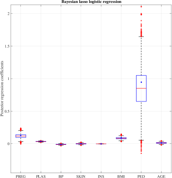
(a) Regression coefficients

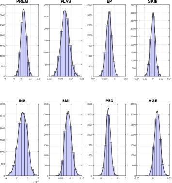
(b) Probability density functions

Figure 1: Bayesian lasso logistic regression analysis of the Pima Indian diabetes data set. A boxplot of the posterior samples of the regression coefficients with the corresponding maximum likelihood estimator (left) and the estimated conditional posterior probability density functions (right).

4 Discussion

The bayesreg toolbox is the only toolbox for Bayesian penalized linear and logistic regression with continuous shrinkage priors that can readily be used for high dimensional problems. It implements linear regression with Gaussian and heavy-tailed error models, as well as logistic regression with the state-of-the-art Pólya-gamma data augmentation strategy. The toolbox supports four different types of continuous shrinkage priors allowing dense models (ridge regression) as well as varying levels of sparsity; e.g., Bayesian lasso for sparse models and horseshoe and horseshoe$+$ for ultra-sparse data. All sampling code is implemented using the Gibbs sampler which could potentially be combined with, for example, Chib’s algorithm [Chib, 1995] for computation of the marginal data likelihood. The toolbox also incorporates a simple metric for ranking of predictors via the $t$ statistic or the Bayesian feature ranking algorithm [Makalic and Schmidt, 2011]. The bayesreg toolbox, complete with full source code, is available for the MATLAB (MATLAB Central File Exchange, File ID #60823) and R (CRAN, package name bayesreg) numerical computing environments. We are also developing a version of bayesreg for the statistical software package Stata.

To date, there are 21 packages on MATLAB Central File Exchange containing the search terms Bayesian regression. Of those, only two packages are in the same domain as bayesreg; one of those packages implements Bayesian lasso linear regression while the other package is on variational Bayes for linear regression. The MATLAB function implementing Bayesian lasso linear regression uses direct matrix inversion to sample the regression coefficients $\bm{\beta}\in\mathbb{R}^{p}$ which is slow, numerically unstable and not suitable for data sets containing more than approximately $100$ predictors. There exist no implementations of Bayesian linear regression with heavy tailed error models, Bayesian logistic regression or the horseshoe and horseshoe$+$ estimators on MATLAB Central File Exchange.

The CRAN repository for R packages contains several implementations of Bayesian shrinkage regression including five packages related to the current toolbox. Of those, three packages implement horseshoe regression with indirect posterior sampling algorithms based on the slice sampler [Gramacy and Pantaleo, 2009, Hahn et al., , Bhattacharya et al., 2016]. The slice sampler by Gramacy and Pantaleo [2009] is implemented in the R package monomvn and is significantly slower than our toolbox. For example, our bayesreg implementation is approximately 40 times faster than monomvn when tested with data where $n=$1,000 and $p=$1,000 [Makalic and Schmidt, 2016] while showing similar, if not better, rates of posterior convergence.

Hahn et al. have proposed an elliptic slice sampler [Murray et al., 2010] for Bayesian linear regression that appears to offer some computational advantages over the Gibbs our sampling approach when applied to the horseshoe estimator. However, unlike our implementation, the elliptical slice sampler can only be used when the sample size is greater than the number of predictors and the design matrix is of full rank. Additionally, the elliptical slice sampler is significantly less flexible than bayesreg and cannot easily be extended to handle grouped variables. In contrast, extension of our latent variable approach to handle multi-level groupings of variables (e.g., genetic markers grouped into genes, and genes grouped into pathways) is straightforward [Xu et al., 2016]. An implementation of this elliptical slice sampler is available in the R package fastHorseshoe.

The package horseshoe Bhattacharya et al. [2016] also uses the slice sampler to implement Bayesian linear regression for the horseshoe estimator. The methodology for sampling of the regression coefficients is efficient and similar to that employed in bayesreg. However, horseshoe only implements Gaussian linear regression and does not allow for alternative prior distributions and error models.

In terms of features, the closest implementation of Bayesian shrinkage regression to our toolbox is the R package rstanarm. This package provides an R interface to the Stan C++ library for Bayesian estimation and features Bayesian shrinkage regression for continuous, binary and count data. The implementation is based on Hamiltonian Monte Carlo combined with the ‘No-U-Turn Sampler’ (NUTS) sampler [Hoffman and Gelman, 2014]. The package provides an interface to Stan implementations of recent shrinkage priors, including the horseshoe, the horseshoe$+$, the Dirichlet–Laplace [Bhattacharya et al., 2015] and the R2–D2 [Zhang et al., 2016] estimator. Unsurprisingly, due to the general nature of Stan, Bayesian shrinkage regression with these priors within Stan is significantly slower than a specialized Gibbs sampler. For example, rstanarm takes approximately 40s to obtain $2,000$ samples for Bayesian horseshoe Gaussian regression using a data set comprising $n=442$ observations and $p=10$ predictors. The equivalent operation takes approximately $0.15$s using the MATLAB version of bayesreg. Furthermore, the NUTS sampler used within Stan appears to sometimes produce divergent MCMC transitions for the horseshoe and horseshoe$+$ estimators [Piironen and Vehtari, 2016].

4.1 Future work

Features planned for future versions of bayesreg include:

• additional prior densities for the regression coefficients, such as the Dirichlet–Laplace [Bhattacharya et al., 2015] and the R2–D2 [Zhang et al., 2016] estimators

• negative binomial regression using the Gaussian scale mixture decomposition of Polson et al. [2013]

• longitudinal (Gaussian) linear regression with the variance–covariance matrix prior distribution proposed by Huang and Wand [2013]

• Bayesian autoregressive noise models [Schmidt and Makalic, 2013]

• grouping of variables to allow better support of categorical (factor) data

• block sampling of regression coefficients for ultra-high-dimensional data sets.

References

- Andrews and Mallows [1974] D. F. Andrews and C. L. Mallows. Scale mixtures of normal distributions. Journal of the Royal Statistical Society (Series B), 36(1):99–102, 1974.
- Armagan et al. [2013] A. Armagan, D. Dunson, and J. Lee. Generalized double Pareto shrinkage. Statistica Sinica, 23(1):119–143, 2013.
- Barndorff-Nielsen et al. [1982] O. Barndorff-Nielsen, J. Kent, and M. Sorensen. Normal variance-mean mixtures and z distributions. International Statistical Review, 50(2):145–159, 1982.
- Bhadra et al. [2016] A. Bhadra, J. Datta, N. G. Polson, and B. Willard. The horseshoe+ estimator of ultra-sparse signals. 2016. arXiv:1502.00560.
- Bhattacharya et al. [2015] A. Bhattacharya, D. Pati, N. S. Pillai, and D. B. Dunson. Dirichlet—Laplace priors for optimal shrinkage. Journal of the American Statistical Association, 110:1479–1490, 2015.
- Bhattacharya et al. [2016] A. Bhattacharya, A. Chakraborty, and B. K. Mallick. Fast sampling with Gaussian scale-mixture priors in high-dimensional regression, 2016. arXiv:1506.04778.
- Breheny and Huang [2011] P. Breheny and J. Huang. Coordinate descent algorithms for nonconvex penalized regression, with applications to biological feature selection. Annals of Applied Statistics, 5(1):232–253, 2011.
- Carvalho et al. [2010] C. M. Carvalho, N. G. Polson, and J. G. Scott. The horseshoe estimator for sparse signals. Biometrika, 97(2):465–480, 2010.
- Chib [1995] S. Chib. Marginal likelihood from the Gibbs output. Journal of the American Statistical Association, 90(432):1313–1321, December 1995.
- Fan and Li [2001] J. Fan and R. Li. Variable selection via nonconcave penalized likelihood and its oracle properties. Journal of the American Statistical Association, 96(456):1348–1360, 2001.
- Friedman et al. [2010] J. Friedman, T. Hastie, and R. Tibshirani. Regularized paths for generalized linear models via coordinate descent. Journal of Statistical Software, 33(1), 2010.
- Frühwirth-Schnatter and Frühwirth [2007] S. Frühwirth-Schnatter and R. Frühwirth. Auxiliary mixture sampling with applications to logistic models. Computational Statistics & Data Analysis, 51, 2007.
- Gelman [2006] A. Gelman. Prior distributions for variance parameters in hierarchical models. Bayesian Analysis, 1(3):515–533, 2006.
- Geman and Geman [1984] S. Geman and D. Geman. Stochastic relaxation, Gibbs distributions, and the Bayesian restoration images. IEEE Tran. Pat. Anal. Mach., 6:721–741, 1984.
- Geyer [1992] C. J. Geyer. Practical markov chain monte carlo. Statistical Science, 7(4):473–483, 1992.
- Gramacy and Pantaleo [2009] R. B. Gramacy and E. Pantaleo. Shrinkage regression for multivariate inference with missing data, and an application to portfolio balancing. 5(2):237–262, 2009.
- Gramacy and Polson [2012] R. B. Gramacy and N. G. Polson. Simulation-based regularized logistic regression. Bayesian Analsyis, 7(3), 2012. URL arXiv:1005.3430v1.
- Griffin and Brown [2010] J. E. Griffin and P. J. Brown. Inference with normal-gamma prior distributions in regression problems. Bayesian Analysis, 5(1):171–188, 2010.
- [19] P. R. Hahn, J. He, and H. Lopes. Elliptical slice sampling for Bayesian shrinkage regression with applications to causal inference. URL http://faculty.chicagobooth.edu/richard.hahn/research.html.
- Hans [2009] C. Hans. Bayesian lasso regression. Biometrika, 96(4):835–845, 2009.
- Hoffman and Gelman [2014] M. D. Hoffman and A. Gelman. The no-u-turn sampler: Adaptively setting path lengths in hamiltonian monte carlo. Journal of Machine Learning Research, 15:1351–1381, 2014.
- Holmes and Held [2006] C. C. Holmes and L. Held. Bayesian auxiliary variable models for binary and multinomial regression. Bayesian Analsyis, 1(1):145–168, 2006.
- Huang and Wand [2013] A. Huang and M. P. Wand. Simple marginally noninformative prior distributions for covariance matrices. Bayesian Analysis, 8(2):439–452, 2013.
- Lichman [2013] M. Lichman. UCI machine learning repository, 2013. URL http://archive.ics.uci.edu/ml.
- Lindley and Smith [1972] D. V. Lindley and A. F. M. Smith. Bayes estimates for the linear model. Journal of the Royal Statistical Society (Series B), 34(1):1–41, 1972.
- Makalic and Schmidt [2011] E. Makalic and D. F. Schmidt. A simple Bayesian algorithm for feature ranking in high dimensional regression problems. In 24th Australasian Joint Conference on Advances in Artificial Intelligence (AIA 2011), volume 7106 of Lecture Notes in Artificial Intelligence, pages 223–230, Perth, Australia, December 5–8 2011.
- Makalic and Schmidt [2016] E. Makalic and D. F. Schmidt. A simple sampler for the horseshoe estimator. IEEE Signal Processing Letters, 23(1):179–182, 2016.
- Murray et al. [2010] I. Murray, R. Adams, and D. MacKay. Elliptical slice sampling. In Thirteenth International Conference on Artificial Intelligence and Statistics, volume 9, pages 541–548, Sardinia, Italy, 2010.
- Park and Casella [2008] T. Park and G. Casella. The Bayesian lasso. Journal of the American Statistical Association, 103(482):681–686, June 2008.
- Piironen and Vehtari [2016] J. Piironen and A. Vehtari. Projection predictive variable selection using stan+r, 2016. URL arXiv:1508.02502.
- Polson and Scott [2010] N. G. Polson and J. G. Scott. Shrink globally, act locally: Sparse Bayesian regularization and prediction. In Bayesian Statistics, volume 9, 2010.
- Polson and Scott [2012] N. G. Polson and J. G. Scott. Local shrinkage rules, Lévy processes and regularized regression. Journal of the Royal Statistical Society (Series B), 74(2):287–311, 2012.
- Polson et al. [2013] N. G. Polson, J. G. Scott, and J. Windle. Bayesian inference for logistic models using Pólya-gamma latent variables. 108(504):1339–1349, 2013.
- Robert and Casella [2004] C. P. Robert and G. Casella. Monte Carlo Statistical Methods. Springer, 2004.
- Rue [2001] H. Rue. Fast sampling of Gaussian markov random fields. Journal of the Royal Statistical Society (Series B), 63(2):325–338, 2001.
- Schmidt and Makalic [2013] D. F. Schmidt and E. Makalic. Estimation of stationary autoregressive models with the Bayesian LASSO. Journal of Time Series Analysis, 34:517–531, 2013.
- Tibshirani [1996] R. Tibshirani. Regression shrinkage and selection via the Lasso. Journal of the Royal Statistical Society (Series B), 58(1):267–288, 1996.
- Tibshirani [2011] R. Tibshirani. Regression shrinkage and selection via the lasso: a retrospective. J. R. Statist. Soc. B, 73:273–282, 2011.
- Windle et al. [2014] J. Windle, N. G. Polson, and J. G. Scott. Sampling Pólya-gamma random variates: alternate and approximate techniques, 2014. URL arXiv:1405.0506 [stat.CO].
- Xu et al. [2016] Z. Xu, D. F. Schmidt, E. Makalic, G. Qian, and J. L. Hopper. Bayesian grouped horseshoe regression with application to additive models. In 29th Australasian Joint Conference on Artificial Intelligence, Hobart, Australia, 2016.
- Zhang [2010] C.-H. Zhang. Nearly unbiased variable selection under minimax concave penalty. The Annals of Statistics, 38(2):894–942, 2010.
- Zhang et al. [2016] Y. Zhang, B. J. Reich, and H. D. Bondell. High dimensional linear regression via the R2–D2 shrinkage prior, 2016. URL arXiv:1609.00046.
- Zou and Hastie [2005] H. Zou and T. Hastie. Regularization and variable selection via the elastic net. Journal of the Royal Statistical Society (Series B), 67(2):301–320, 2005.