On the notions of
facets, weak facets, and extreme functions
of the Gomory–Johnson infinite group problem

Abstract

We investigate three competing notions that generalize the notion of a facet of finite-dimensional polyhedra to the infinite-dimensional Gomory–Johnson model. These notions were known to coincide for continuous piecewise linear functions with rational breakpoints. We show that two of the notions, extreme functions and facets, coincide for the case of continuous piecewise linear functions, removing the hypothesis regarding rational breakpoints. We then separate the three notions using discontinuous examples.

1 Introduction

1.1 Facets in the finite-dimensional case

Let $G$ be a finite index set. The space $\mathbb{R}^{(G)}$ of real-valued functions $y\colon G\to\mathbb{R}$ is isomorphic to and routinely identified with the Euclidean space $\mathbb{R}^{|G|}$. Let $\mathbb{R}^{G}$ denote its dual space. It is the space of functions $\alpha\colon G\to\mathbb{R}$, which we consider as linear functionals on $\mathbb{R}^{(G)}$ via the pairing $\langle\alpha,y\rangle=\sum_{r\in G}\alpha(r)y(r)$. Again it is routinely identified with the Euclidean space $\mathbb{R}^{|G|}$, and the dual pairing $\langle\alpha,y\rangle$ is the Euclidean inner product. A (closed, convex) rational polyhedron of $\mathbb{R}^{(G)}$ is the set of $y\colon G\to\mathbb{R}$ satisfying $\langle\alpha_{i},y\rangle\geq\alpha_{i,0}$, where $\alpha_{i}\in\mathbb{Z}^{G}$ are integer linear functionals and $\alpha_{i,0}\in\mathbb{Z}$, for $i$ ranging over another finite index set $I$.

Consider an integer linear optimization problem in $\mathbb{R}^{(G)}$, i.e., the problem of minimizing a linear functional $\eta\in\mathbb{R}^{G}$ over a feasible set $F\subseteq\{\,y\colon G\to\mathbb{Z}_{+}\,\}\subset\mathbb{R}_{+}^{(G)}$, or, equivalently, over the convex hull $R=\operatorname{conv}F\subset\mathbb{R}_{+}^{(G)}$. A valid inequality for $R$ is an inequality of the form $\langle\pi,y\rangle\geq\pi_{0}$, where $\pi\in\mathbb{R}^{G}$, which holds for all $y\in R$ (equivalently, for all $y\in F$). If $R$ is closed and convex, it is exactly the set of all $y$ that satisfy all valid inequalities. In the following we will restrict ourselves to the case that $R\subseteq\mathbb{R}_{+}^{(G)}$ is a polyhedron of blocking type, in which case we only need to consider normalized valid inequalities with $\pi\geq 0$ and $\pi_{0}=1$.

Let $P(\pi)$ denote the set of functions $y\in F$ for which the inequality $\langle\pi,y\rangle\geq 1$ is tight, i.e., $\langle\pi,y\rangle=1$. If $P(\pi)\neq\emptyset$, then $\langle\pi,y\rangle\geq 1$ is a tight valid inequality. Then $R$ is exactly the set of all $y\geq 0$ that satisfy all tight valid inequalities. A valid inequality $\langle\pi,y\rangle\geq 1$ is called minimal if there is no other valid inequality $\pi^{\prime}\neq\pi$ such that $\pi^{\prime}\leq\pi$ pointwise. One can show that a minimal valid inequality is tight. A valid inequality $\langle\pi,y\rangle\geq 1$ is called facet-defining if

$$\text{for every valid inequality $\langle\pi^{\prime},y\rangle\geq 1$ such that $P(\pi)\subseteq P(\pi^{\prime})$},$$ (wF)

we have $$P(\pi)=P(\pi^{\prime})$$,

or, in other words, if the face induced by $\langle\pi,y\rangle\geq 1$ is maximal. Under the above assumptions, $R$ has full affine dimension. Thus, we get the following characterization of facet-defining inequalities:

$$\text{for every valid inequality $\langle\pi^{\prime},y\rangle\geq 1$ such that $P(\pi)\subseteq P(\pi^{\prime})$},$$ (F)

we have $$\pi=\pi^{\prime}$$.

The theory of polyhedra gives another characterization of facets:

If $$\langle\pi^{1},y\rangle\geq 1 \langle\pi^{2},y\rangle\geq 1 \pi=\tfrac{1}{2}(\pi^{1}+\pi^{2})$$ and are valid inequalities, and (E)

$$\text{then $\pi=\pi^{1}=\pi^{2}$}.$$

1.2 Facets in the infinite-dimensional Gomory–Johnson model

It is perhaps not surprising that the three conditions (wF), (F), and (E) are no longer equivalent when $R$ is a general convex set that is not polyhedral, and in particular when we change from the finite-dimensional to the infinite-dimensional case. In the present paper, however, we consider a particular case of an infinite-dimensional model, in which this question has eluded researchers for a long time. Let $G=\mathbb{Q}$ or $G=\mathbb{R}$ and let $\mathbb{R}^{(G)}$ now denote the space of finite-support functions $y\colon G\to\mathbb{R}$. The so-called infinite group problem was introduced by Gomory and Johnson in their seminal papers [12, 13]. Let $F=F_{f}(G,\mathbb{Z})\subseteq\mathbb{R}_{+}^{(G)}$ be the set of all finite-support functions $y\colon G\to\mathbb{Z}_{+}$ satisfying the equation

$$\sum_{r\in G}r\,y(r)\equiv f\pmod{1}$$ (1)

where $f$ is a given element of $G\setminus\mathbb{Z}$. We study its convex hull $R=R_{f}(G,\mathbb{Z})\subseteq\mathbb{R}_{+}^{(G)}$, whose elements are understood as finite-support functions $y\colon G\to\mathbb{R}_{+}$.

Valid inequalities for $R$ are of the form $\langle\pi,y\rangle\geq\pi_{0}$, where $\pi$ comes from the dual space $\mathbb{R}^{G}$, which is the space of all real-valued functions (without the finite-support condition). When $G=\mathbb{Q}$, then $R$ is again of “blocking type” (see, for example, [8, section 5]), and so we again may assume $\pi\geq 0$ and $\pi_{0}=1$.

If $G=\mathbb{R}$ (the setting of the present paper), typical pathologies from the analysis of functions of a real variable come into play. For example, by [5, Proposition 2.4] there is an infinite-dimensional space of valid equations $\langle\pi^{*},y\rangle=0$, where $\pi^{*}$ are constructed using a Hamel basis of $\mathbb{R}$ over $\mathbb{Q}$. Each of these functions $\pi^{*}$ has a graph whose topological closure is $\mathbb{R}^{2}$. In order to tame these pathologies, it is common to make further assumptions. Gomory–Johnson [12, 13] only considered continuous functions $\pi$. However, this rules out many interesting functions such as the Gomory fractional cut. Instead it has become common in the literature to build the assumption $\pi\geq 0$ into the definition; then we can again normalize $\pi_{0}=1$. We call such functions $\pi$ valid functions.

(Minimal) valid functions $\pi$ that satisfy the conditions (wF), (F), and (E), are called weak facets, facets, and extreme functions, respectively. The relation of these notions, in particular of facets and extreme functions, has remained unclear in the literature. For example, Basu et al. [2] wrote:

The statement that extreme functions are facets appears to be quite nontrivial to prove, and to the best of our knowledge there is no proof in the literature. We therefore cautiously treat extreme functions and facets as distinct concepts, and leave their equivalence as an open question.

We refer to [5, section 2.2] for further discussion.

1.3 Contribution of this paper

A well known sufficient condition for facetness of a minimal valid function $\pi$ is the Gomory–Johnson Facet Theorem. In its strong form, due to Basu–Hildebrand–Köppe–Molinaro [7], it reads:

Theorem 1.1 (Facet Theorem, strong form, [7, Lemma 34]; see also [5, Theorem 2.12])

Suppose for every minimal valid function $\pi^{\prime}$, $E(\pi)\subseteq E(\pi^{\prime})$ implies $\pi^{\prime}=\pi$. Then $\pi$ is a facet.

(Here $E(\pi)$ is the additivity domain of $\pi$, defined in section 2.) We show (Theorem 4.1 below) that, in fact, this holds as an “if and only if” statement.

For the case of continuous piecewise linear functions with rational breakpoints, Basu et al. [5, Proposition 2.8] showed that the notions of extreme functions and facets coincide. This was a consequence of Basu et al.’s finite oversampling theorem [3]. We sharpen this result by removing the hypothesis regarding rational breakpoints.

Theorem 1.2

In the case of continuous piecewise linear functions (not necessarily with rational breakpoints), $\{$extreme functions$\}=\{$facets$\}$.

Then we investigate the notions of facets and weak facets in the case of discontinuous functions. This appears to be a first in the published literature. All papers that consider discontinuous functions only used the notion of extreme functions; see Appendix 0.A for a discussion. We give three discontinuous functions that furnish the separation of the three notions (Theorem 6.1): A function $\psi$ that is extreme, but is neither a weak facet nor a facet; a function $\pi$ that is not an extreme function (nor a facet), but is a weak facet; and a function $\pi_{\mathrm{lifted}}$ that is extreme and a weak facet but is not a facet.

It remains an open question whether this separation can also be done using continuous (non–piecewise linear) functions.

2 Minimal valid functions and their perturbations

Following [5], given a locally finite one-dimensional polyhedral complex $\mathcal{P}$, we call a function $\pi\colon\mathbb{R}\to\mathbb{R}$ piecewise linear over $\mathcal{P}$, if it is affine linear over the relative interior of each face of the complex. Under this definition, piecewise linear functions can be discontinuous. We say the function $\pi$ is continuous piecewise linear over $\mathcal{P}$ if it is affine over each of the cells of $\mathcal{P}$ (thus automatically imposing continuity).

Let $\pi$ be a minimal valid function. Define the subadditivity slack of $\pi$ as $\Delta\pi(x,y):=\pi(x)+\pi(y)-\pi(x+y)$. Denote the additivity domain of $\pi$ by

$$E(\pi)=\{(x,y)\mid\Delta\pi(x,y)=0\}.$$

To combinatorialize the additivity domains of piecewise linear subadditive functions, we work with the two-dimensional polyhedral complex $\Delta\mathcal{P}$, whose faces are $F(I,J,K)=\{(x,y)\in\mathbb{R}\times\mathbb{R}\mid x\in I,y\in J,x+y\in K\}$ for $I,J,K\in\mathcal{P}$. Define the projections $p_{1},p_{2},p_{3}\colon\mathbb{R}\times\mathbb{R}\to\mathbb{R}$ as $p_{1}(x,y)=x$, $p_{2}(x,y)=y$, $p_{3}(x,y)=x+y$.

In the continuous case, since the function $\pi$ is piecewise linear over $\mathcal{P}$, we have that $\Delta\pi$ is affine linear over each face $F\in\Delta P$. Let $\pi$ be a minimal valid function for $R_{f}(\mathbb{R},\mathbb{Z})$ that is piecewise linear over $\mathcal{P}$. Following [5], we define the space of perturbation functions with prescribed additivities $E=E(\pi)$

$$\bar{\Pi}^{E}(\mathbb{R},\mathbb{Z})=\left\{\bar{\pi}\colon\mathbb{R}\to\mathbb{R}\,\Bigg{|}\,\begin{array}[]{r@{\;}c@{\;}ll}\bar{\pi}(0)&=&0\\ \bar{\pi}(f)&=&0\\ \bar{\pi}(x)+\bar{\pi}(y)&=&\bar{\pi}(x+y)&\text{ for all }(x,y)\in E\\ \bar{\pi}(x)&=&\bar{\pi}(x+t)&\text{ for all }x\in\mathbb{R},\,t\in\mathbb{Z}\end{array}\right\}.$$ (2)

When $\pi$ is discontinuous, one also needs to consider the limit points where the subadditivity slacks are approaching zero. Let $F$ be a face of $\Delta\mathcal{P}$. For $(x,y)\in F$, we denote

$$\Delta\pi_{F}(x,y):=\lim_{\begin{subarray}{c}(u,v)\to(x,y)\\ (u,v)\in\operatorname{rel\,int}(F)\end{subarray}}\Delta\pi(u,v).$$

Define

$$E_{F}(\pi)=\{\,(x,y)\in F\mid\Delta\pi_{F}(x,y)\text{ exists, and }\Delta\pi_{F}(x,y)=0\,\}.$$

Notice that in the above definition of $E_{F}(\pi)$, we include the condition that the limit denoted by $\Delta\pi_{F}(x,y)$ exists, so that this definition can as well be applied to functions $\pi$ (and $\bar{\pi}$) that are not piecewise linear over $\mathcal{P}$.

We denote by $E_{\bullet}(\pi,\mathcal{P})$ the family of sets $E_{F}(\pi)$, indexed by $F\in\Delta\mathcal{P}$. Define the space of perturbation functions with prescribed additivities and limit-additivities $E_{\bullet}=E_{\bullet}(\pi,\mathcal{P})$

$$\bar{\Pi}^{E_{\bullet}}(\mathbb{R},\mathbb{Z})=\left\{\bar{\pi}\colon\mathbb{R}\to\mathbb{R}\,\Bigg{|}\,\begin{array}[]{r@{\;}c@{\;}ll}\bar{\pi}(0)&=&0\\ \bar{\pi}(f)&=&0\\ \Delta\bar{\pi}_{F}(x,y)&=&0&\text{ for }(x,y)\in E_{F},\ F\in\Delta\mathcal{P}\\ \bar{\pi}(x)&=&\bar{\pi}(x+t)&\text{ for }x\in\mathbb{R},\,t\in\mathbb{Z}\end{array}\right\}.$$ (3)

Remark 1

Let $\bar{\pi}\in\bar{\Pi}^{E}(\mathbb{R},\mathbb{Z})$. The third condition of (2) is equivalent to $E(\pi)\subseteq E(\bar{\pi})$. Let $\bar{\pi}\in\bar{\Pi}^{E_{\bullet}}(\mathbb{R},\mathbb{Z})$. The third condition of (3) is equivalent to $E_{F}(\pi)\subseteq E_{F}(\bar{\pi})$ for all faces $F\in\Delta\mathcal{P}$, which is stronger than $E(\pi)\subseteq E(\bar{\pi})$ in (2). Thus, in general, $\bar{\Pi}^{E_{\bullet}}(\mathbb{R},\mathbb{Z})\subseteq\bar{\Pi}^{E}(\mathbb{R},\mathbb{Z})$. If $\pi$ is continuous, then $E(\pi)\subseteq E(\bar{\pi})$ implies that $E_{F}(\pi)\subseteq E_{F}(\bar{\pi})$ for all faces $F\in\Delta\mathcal{P}$, hence $\bar{\Pi}^{E_{\bullet}}(\mathbb{R},\mathbb{Z})=\bar{\Pi}^{E}(\mathbb{R},\mathbb{Z})$.

3 Effective perturbation functions

Following [16], we define the space of effective perturbation functions

$$\tilde{\Pi}^{\pi}(\mathbb{R},\mathbb{Z})=\left\{\,\tilde{\pi}\colon\mathbb{R}\to\mathbb{R}\,\mid\,\exists\,\epsilon>0\text{ s.t.\ }\pi^{\pm}=\pi\pm\epsilon\tilde{\pi}\text{ are minimal valid}\,\right\}.$$ (4)

Because of [5, Lemma 2.11 (i)], a function $\pi$ is extreme if and only if $\tilde{\Pi}^{\pi}(\mathbb{R},\mathbb{Z})=\left\{0\right\}$. Note that every function $\tilde{\pi}\in\tilde{\Pi}^{\pi}(\mathbb{R},\mathbb{Z})$ is bounded.

It is clear that if $\tilde{\pi}\in\tilde{\Pi}^{\pi}(\mathbb{R},\mathbb{Z})$, then $\tilde{\pi}\in\bar{\Pi}^{E_{\bullet}}(\mathbb{R},\mathbb{Z})$, where $E_{\bullet}=E_{\bullet}(\pi,\mathcal{P})$; see [3, Lemma 2.7] or [16, Lemma LABEL:crazy:lemma:tight-implies-tight].

The other direction does not hold in general, but requires additional hypotheses. Let $\bar{\pi}\in\bar{\Pi}^{E_{\bullet}}(\mathbb{R},\mathbb{Z})$. In [4, Theorem 3.13] (see also [5, Theorem 3.13]), it is proved that if $\pi$ and $\bar{\pi}$ are continuous and $\bar{\pi}$ is piecewise linear, we have $\bar{\pi}\in\tilde{\Pi}^{\pi}(\mathbb{R},\mathbb{Z})$. (Similar arguments also appeared in the earlier literature, for example in the proof of [3, Theorem 3.2].)

We will need a more general version of this result. Consider the following definition. Given a locally finite one-dimensional polyhedral complex $\mathcal{P}$, we call a function $\bar{\pi}\colon\mathbb{R}\to\mathbb{R}$ piecewise Lipschitz continuous over $\mathcal{P}$, if it is Lipschitz continuous over the relative interior of each face of the complex. Under this definition, piecewise Lipschitz continuous functions can be discontinuous.

Theorem 3.1

Let $\pi$ be a minimal valid function that is piecewise linear over a polyhedral complex $\mathcal{P}$. Let $\bar{\pi}\in\bar{\Pi}^{E_{\bullet}}(\mathbb{R},\mathbb{Z})$ be a perturbation function, where $E_{\bullet}=E_{\bullet}(\pi,\mathcal{P})$. Suppose that $\bar{\pi}$ is piecewise Lipschitz continuous over $\mathcal{P}$. Then $\bar{\pi}$ is an effective perturbation function, $\bar{\pi}\in\tilde{\Pi}^{\pi}(\mathbb{R},\mathbb{Z})$.

The proof appears in Appendix 0.B.

4 Extreme functions and facets

In this section, we discuss the relations between the notions of extreme functions and facets. We first review the definition of a facet, following [5, section 2.2.3]; cf. ibid. for a discussion of this notion in the earlier literature, in particular [14] and [10].

Let $P(\pi)$ denote the set of functions $y\colon\mathbb{R}\to\mathbb{Z}_{+}$ with finite support satisfying

$$\sum_{r\in\mathbb{R}}ry(r)\in f+\mathbb{Z}\quad\text{ and }\quad\sum_{r\in\mathbb{R}}\pi(r)y(r)=1.$$

A valid function $\pi$ is called a facet if for every valid function $\pi^{\prime}$ such that $P(\pi)\subseteq P(\pi^{\prime})$ we have that $\pi^{\prime}=\pi$. Equivalently, a valid function $\pi$ is a facet if this condition holds for all such minimal valid functions $\pi^{\prime}$ [7].

Remark 2

In the discontinuous case, the additivity in the limit plays a role in extreme functions, which are characterized by the non-existence of an effective perturbation function $\tilde{\pi}\not\equiv 0$. However facets (and weak facets, see the next section) are defined through $P(\pi)$, which does not capture the limiting additive behavior of $\pi$. The additivity domain $E(\pi)$, which features in the Facet Theorem as discussed below, also does not account for additivity in the limit.

A well known sufficient condition for facetness of a minimal valid function $\pi$ is the Gomory–Johnson Facet Theorem. We have stated its strong form, due to Basu–Hildebrand–Köppe–Molinaro [7], in the introduction as Theorem 1.1. In order to prove our “if and only if” version, we need the following lemma.

Lemma 1

Let $\pi$ and $\pi^{\prime}$ be minimal valid functions. Then $E(\pi)\subseteq E(\pi^{\prime})$ if and only if $P(\pi)\subseteq P(\pi^{\prime})$.

Proof

The “if” direction is proven in [7, Theorem 20]; see also [5, Theorem 2.12]. We now show the “only if” direction, using the subadditivity of $\pi$. Assume that $E(\pi)\subseteq E(\pi^{\prime})$. Let $y\in P(\pi)$. Let $\{r_{1},r_{2},\dots,r_{n}\}$ denote the finite support of $y$. By definition, the function $y$ satisfies that $y(r_{i})\in\mathbb{Z}_{+}$, $\sum_{i=1}^{n}r_{i}y(r_{i})\equiv f\pmod{1}$, and $\sum_{i=1}^{n}\pi(r_{i})y(r_{i})=1$. Since $\pi$ is a minimal valid function, we have that $1=\sum_{i=1}^{n}\pi(r_{i})y(r_{i})\geq\pi(\sum_{i=1}^{n}r_{i}y(r_{i}))=\pi(f)=1.$ Thus, each subadditivity inequality here is tight for $\pi$, and is also tight for $\pi^{\prime}$ since $E(\pi)\subseteq E(\pi^{\prime})$. We obtain $\sum_{i=1}^{n}\pi^{\prime}(r_{i})y(r_{i})=\pi^{\prime}(\sum_{i=1}^{n}r_{i}y(r_{i}))=\pi^{\prime}(f)=1,$ which implies that $y\in P(\pi^{\prime})$. Therefore, $P(\pi)\subseteq P(\pi^{\prime})$.

Theorem 4.1 (Facet Theorem, “if and only if” version)

A minimal valid function $\pi$ is a facet if and only if for every minimal valid function $\pi^{\prime}$, $E(\pi)\subseteq E(\pi^{\prime})$ implies $\pi^{\prime}=\pi$.

Proof

It follows from the Facet Theorem in the strong form (Theorem 1.1) and 1.

In [5, page 25, section 3.6], the Facet Theorem is reformulated in terms of perturbation functions. In Appendix 0.C we prove an “if and only if” result for this reformulation as well.

Now we come to the proof of a main theorem stated in the introduction.

Proof (of Theorem 1.2)

Let $\pi$ be a continuous piecewise linear minimal valid function. As mentioned in [5, section 2.2.4], [7, Lemma 1.3] showed that if $\pi$ is a facet, then $\pi$ is extreme.

We now prove the other direction by contradiction. Suppose that $\pi$ is extreme, but is not a facet. Then by Theorem 4.1, there exists a minimal valid function $\pi^{\prime}\neq\pi$ such that $E(\pi)\subseteq E(\pi^{\prime})$. Since $\pi$ is continuous piecewise linear and $\pi(0)=\pi(1)=0$, there exists $\delta>0$ such that $\Delta\pi(x,y)=0$ and $\Delta\pi(-x,-y)=0$ for $0\leq x,y\leq\delta$. The condition $E(\pi)\subseteq E(\pi^{\prime})$ implies that $\Delta\pi^{\prime}(x,y)=0$ and $\Delta\pi^{\prime}(-x,-y)=0$ for $0\leq x,y\leq\delta$ as well. As the function $\pi^{\prime}$ is bounded, it follows from the Interval Lemma (see [5, Lemma 4.1], for example) that $\pi^{\prime}$ is affine linear on $[0,\delta]$ and on $[-\delta,0]$. We also know that $\pi^{\prime}(0)=0$ as $\pi^{\prime}$ is minimal valid. Using the subadditivity, we obtain that $\pi^{\prime}$ is Lipschitz continuous. Let $\bar{\pi}=\pi^{\prime}-\pi$. Then $\bar{\pi}\not\equiv 0$, $\bar{\pi}\in\bar{\Pi}^{E}(\mathbb{R},\mathbb{Z})$ where $E=E(\pi)$, and $\bar{\pi}$ is Lipschitz continuous. Since $\pi$ is continuous, we have $\bar{\Pi}^{E}(\mathbb{R},\mathbb{Z})=\bar{\Pi}^{E_{\bullet}}(\mathbb{R},\mathbb{Z})$. By Theorem 3.1, there exists $\epsilon>0$ such that $\pi^{\pm}=\pi\pm\epsilon\bar{\pi}$ are distinct minimal valid functions. This contradicts the assumption that $\pi$ is an extreme function.

Therefore, $\{$extreme functions$\}=\{$facets$\}$.

5 Weak facets

We first review the definition of a weak facet, following [5, section 2.2.3]; cf. ibid. for a discussion of this notion in the earlier literature, in particular [14] and [10]. A valid function $\pi$ is called a weak facet if for every valid function $\pi^{\prime}$ such that $P(\pi)\subseteq P(\pi^{\prime})$ we have $P(\pi)=P(\pi^{\prime})$.

As we mentioned above, to prove that $\pi$ is an extreme function or is a facet, it suffices to consider $\pi^{\prime}$ that is minimal valid. The following lemma shows it is also the case in the definition of weak facets.

Lemma 2

1. Let $\pi$ be a valid function. If $\pi$ is a weak facet, then $\pi$ is minimal valid.

2. Let $\pi$ be a minimal valid function. Suppose that for every minimal valid function $\pi^{\prime}$, we have that $P(\pi)\subseteq P(\pi^{\prime})$ implies $P(\pi)=P(\pi^{\prime})$. Then $\pi$ is a weak facet.

3. A minimal valid function $\pi$ is a weak facet if and only if for every minimal valid function $\pi^{\prime}$, we have that $E(\pi)\subseteq E(\pi^{\prime})$ implies $E(\pi)=E(\pi^{\prime})$.

Proof

(1) Suppose that $\pi$ is not minimal valid. Then, by [7, Theorem 1], $\pi$ is dominated by another minimal valid function $\pi^{\prime}$, with $\pi(x_{0})>\pi^{\prime}(x_{0})$ at some $x_{0}$. Let $y\in P(\pi)$. We have

$$1=\sum\pi(r_{i})y(r_{i})\geq\sum\pi^{\prime}(r_{i})y(r_{i})\geq\pi^{\prime}(\sum r_{i}y(r_{i}))=\pi^{\prime}(f)=1.$$

Hence equality holds throughout, implying that $y\in P(\pi^{\prime})$. Therefore, $P(\pi)\subseteq P(\pi^{\prime})$. Now consider $y$ with $y(x_{0})=y(f-x_{0})=1$ and $y(x)=0$ otherwise. It is easy to see that $y\in P(\pi^{\prime})$, but $y\not\in P(\pi)$ since $\pi(x_{0})+\pi(f-x_{0})>\pi^{\prime}(x_{0})+\pi^{\prime}(f-x_{0})=1$. Therefore, $P(\pi)\subsetneq P(\pi^{\prime})$, a contradiction to the weak facet assumption on $\pi$.

(2) Consider any valid function $\pi^{*}$ (not necessarily minimal) such that $P(\pi)\subseteq P(\pi^{*})$. Let $\pi^{\prime}$ be a minimal function that dominates $\pi^{*}$: $\pi^{\prime}\leq\pi^{*}$. From (1) we know that $P(\pi^{*})\subseteq P(\pi^{\prime})$. Thus, $P(\pi)\subseteq P(\pi^{\prime})$. By hypothesis, we have that $P(\pi)=P(\pi^{*})=P(\pi^{\prime})$. Therefore, $\pi$ is a weak facet.

(3) Direct consequence of (2) and 1.

Theorem 5.1

Let $\mathcal{F}$ be a family of functions such that existence of an effective perturbation implies existence of a piecewise linear effective perturbation. Let $\pi$ be a continuous piecewise linear function (not necessarily with rational breakpoints) such that $\pi\in\mathcal{F}$. The following are equivalent. (1) $\pi$ is extreme, (2) $\pi$ is a facet, (3) $\pi$ is a weak facet.

Remark 3

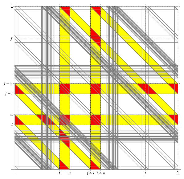
Figure 2: Diagram of the polyhedral complex $\Delta\mathcal{P}$ of the function $\pi=\texttt{kzh\char 95\relax\allowbreak minimal\char 95\relax\allowbreak has\char 95\relax\allowbreak only\char 95\relax\allowbreak crazy\char 95\relax\allowbreak perturbation\char 95\relax\allowbreak 1()}$, where faces $F$ are color-coded according to the values $n_{F}$: $n_{F}=0$ (white), $n_{F}=1$ (yellow), $n_{F}=2$ (red).

In general, facets form a subset of the intersection of extreme functions and weak facets. In the case of continuous piecewise linear functions with rational breakpoints, [5, Proposition 2.8] and [6, Theorem 8.6] proved that “extreme $\Leftrightarrow$ facet”. Note that in this case, “weak facet $\Rightarrow$ facet” can be shown by restriction with oversampling to finite group problems. Thus (1), (2), (3) are equivalent when $\pi$ is a continuous piecewise linear function with rational breakpoints. See [5, Figure 2] for an illustration. As shown in [3] (for a stronger statement, see [6, Theorem 8.6]), the family of continuous piecewise linear function with rational breakpoints is such a family $\mathcal{F}$ where existence of an effective perturbation implies existence of a piecewise linear effective perturbation. A forthcoming paper will investigate larger such families $\mathcal{F}$.

Proof (of Theorem 5.1)

By Theorem 1.2 and the fact that $\{$facets$\}\subseteq\{$extreme functions$\}\cap\{$weak facets$\}$, it suffices to show that $\{$weak facets$\}\subseteq\{$extreme functions$\}$.

Assume that $\pi$ is a weak facet, thus $\pi$ is minimal valid by 2. We show that $\pi$ is extreme. For the sake of contradiction, suppose that $\pi$ is not extreme. By the assumption $\pi\in\mathcal{F}$, there exists a piecewise linear perturbation function $\bar{\pi}\not\equiv 0$ such that $\pi\pm\bar{\pi}$ are minimal valid functions. Furthermore, by [5, Lemma 2.11], we know that $\bar{\pi}$ is continuous, and $E(\pi)\subseteq E(\bar{\pi})$. By taking the union of the breakpoints, we can define a common refinement, which will still be denoted by $\mathcal{P}$, of the complexes for $\pi$ and for $\bar{\pi}$. In other words, we may assume that $\pi$ and $\bar{\pi}$ are both continuous piecewise linear over $\mathcal{P}$. Since $\Delta\bar{\pi}\not\equiv 0$, we may assume without loss of generality that $\Delta\bar{\pi}(x,y)>0$ for some $(x,y)\in\operatorname{vert}(\Delta\mathcal{P})$. Define

$$\epsilon=\min\left\{\frac{\Delta\pi(x,y)}{\Delta\bar{\pi}(x,y)}\mid(x,y)\in\operatorname{vert}(\Delta\mathcal{P}),\Delta\bar{\pi}(x,y)>0\right\}.$$

Notice that $\epsilon>0$, since $\Delta\pi\geq 0$ and $E(\pi)\subseteq E(\bar{\pi})$. Let $\pi^{\prime}=\pi-\epsilon\bar{\pi}$. Then $\pi^{\prime}$ is a bounded continuous function piecewise linear over $\mathcal{P}$, such that $\pi^{\prime}\neq\pi$.

The function $\pi^{\prime}$ is subadditive, since $\Delta\pi^{\prime}(x,y)\geq 0$ for each $(x,y)\in\operatorname{vert}(\Delta\mathcal{P})$. As in the proof of Theorem 3.1, it can be shown that $\pi^{\prime}$ is non-negative, $\pi^{\prime}(0)=0$, $\pi^{\prime}(f)=1$, and that $\pi^{\prime}$ satisfies the symmetry condition. Therefore, $\pi^{\prime}$ is a minimal valid function. Let $(u,v)$ be a vertex of $\Delta\mathcal{P}$ satisfying $\Delta\bar{\pi}(u,v)>0$ and $\Delta\pi(u,v)=\epsilon\Delta\bar{\pi}(u,v)$. We know that $\Delta\pi^{\prime}(u,v)=\Delta\pi(u,v)-\epsilon\Delta\bar{\pi}(u,v)=0$, hence $(u,v)\in E(\pi^{\prime})$. However, $(u,v)\not\in E(\pi)$, since $\Delta\bar{\pi}(u,v)>0$ implies that $\Delta\pi(u,v)\neq 0$. Therefore, $E(\pi)\subsetneq E(\pi^{\prime})$. By 2(3), we have that $\pi$ is not a weak facet, a contradiction.

6 Separation of the notions in the discontinuous case

The definition of facets fails to account for additivities-in-the-limit, which are a crucial feature of the extremality test for discontinuous functions. This allows us to separate the two notions. Below we do this by observing that a discontinuous piecewise linear extreme function from the literature, hildebrand_discont_3_slope_1(), constructed by Hildebrand (2013, unpublished; reported in [5]), works as a separating example.

The other separations appear to require more complicated constructions. Recently, the authors constructed a two-sided discontinuous piecewise linear minimal valid function, kzh_minimal_has_only_crazy_perturbation_1, which is not extreme, but which is not a convex combination of other piecewise linear minimal valid functions; see [16] for the definition. This function has two special “uncovered” pieces on the intervals $(l,u)$ and $(f-u,f-l)$, where $f=\frac{4}{5}$, $l=\frac{219}{800}$, $u=\frac{269}{800}$, on which every nonzero perturbation is microperiodic (invariant under the action of the dense additive group $T=\langle t_{1},t_{2}\rangle_{\mathbb{Z}}$, where $t_{1}=\frac{77}{7752}\sqrt{2}$, $t_{2}=\frac{77}{2584}$). Below we prove that it furnishes another separation.

For the remaining separation, we construct an extreme function $\pi_{\mathrm{lifted}}$ as follows. Define $\pi_{\mathrm{lifted}}$ by perturbing the function $\pi=\texttt{kzh\char 95\relax\allowbreak minimal\char 95\relax\allowbreak has\char 95\relax\allowbreak only\char 95\relax\allowbreak}$crazy_perturbation_1() on infinitely many cosets of the group $T$ on the two uncovered intervals as follows.

$$\pi_{\mathrm{lifted}}(x)=\begin{cases}\pi(x)&\text{if }x\not\in(l,u)\cup(f-u,f-l)\text{, or}\\ &\text{if }x\in(l,u)\text{ such that }x\in C\text{, or}\\ &\text{if }x\in(f-u,f-l)\text{ such that }f-x\in C;\\ \pi(x)+s&\text{if }x\in(l,u)\text{ such that }x\in C^{+}\text{, or}\\ &\text{if }x\in(f-u,f-l)\text{ such that }f-x\in C^{+};\\ \pi(x)-s&\text{otherwise},\end{cases}$$ (5)

where $x_{39}=\frac{4899}{5000}$, $s=\pi(x_{39}^{-})+\pi(1+l-x_{39})-\pi(l)=\frac{19}{23998}$,

$$C =\{x\in\mathbb{R}/T\mid x=\tfrac{l+u}{2}\text{ or }\tfrac{l+u-t_{1}}{2}\text{ or }\tfrac{l+u-t_{2}}{2}\},$$

$$C^{+} =\{x\in\mathbb{R}/T\mid\text{arbitrary choice of one element of }\{x,\phi(x)\},\,x\not\in C\}$$

with $\phi\colon\mathbb{R}/T\ni x\mapsto l+u-x$.

Theorem 6.1

1. The function $\psi=\texttt{hildebrand\char 95\relax\allowbreak discont\char 95\relax\allowbreak 3\char 95\relax\allowbreak slope\char 95\relax\allowbreak 1()}$ is extreme, but is neither a weak facet nor a facet.

2. The function $\pi=\texttt{kzh\char 95\relax\allowbreak minimal\char 95\relax\allowbreak has\char 95\relax\allowbreak only\char 95\relax\allowbreak crazy\char 95\relax\allowbreak perturbation\char 95\relax\allowbreak 1()}$ is not an extreme function (nor a facet), but is a weak facet.

3. The function $\pi_{\mathrm{lifted}}$ is extreme; it is a weak facet but is not a facet.

Proof

(1) The function $\psi=\texttt{hildebrand\char 95\relax\allowbreak discont\char 95\relax\allowbreak 3\char 95\relax\allowbreak slope\char 95\relax\allowbreak 1()}$ is extreme (Hildebrand, 2013, unpublished, reported in [5]). This can be verified using the extremality test implemented in [15]. Consider the minimal valid function $\pi^{\prime}$ defined by

$$\pi^{\prime}(x)=\begin{cases}2x&\text{if }x\in[0,\frac{1}{2}];\\ \pi(x)&\text{if }x\in(\frac{1}{2},1).\end{cases}$$

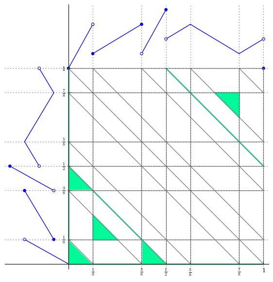
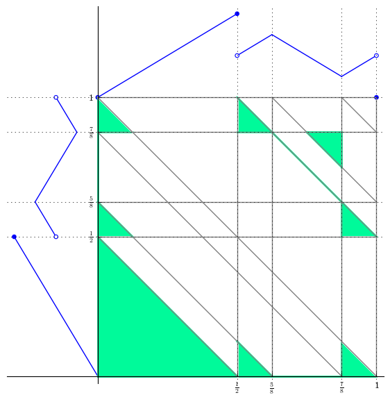
Figure 1: Two diagrams of functions h (blue graphs on the top and the left) and polyhedral complexes $\Delta\mathcal{P}$ (gray solid lines) with additive domains $E(\texttt{h})$ (shaded in green), as plotted by the command plot_2d_diagram_additive_domain_sans_limits(h). (Left) $\texttt{h = hildebrand\char 95\relax\allowbreak discont\char 95\relax\allowbreak 3\char 95\relax\allowbreak slope\char 95\relax\allowbreak 1()}=\pi$. (Right) h $=\pi^{\prime}$ from the proof of Theorem 6.1 (2).

Observe that $E(\psi)$ is a strict subset of $E(\pi^{\prime})$. See Figure 1 for an illustration. Thus, by 2(3), the function $\psi$ is not a weak facet (nor a facet).

(2) By [16, Theorem LABEL:crazy:th:kzh_minimal_has_only_crazy_perturbation_1], the function $\pi=\texttt{kzh\char 95\relax\allowbreak minimal\char 95\relax\allowbreak has\char 95\relax\allowbreak only\char 95\relax\allowbreak crazy\char 95\relax\allowbreak}$perturbation_1() is minimal valid, but is not extreme. Let $\pi^{\prime}$ be a minimal valid function such that $E(\pi)\subseteq E(\pi^{\prime})$. We want to show that $E(\pi)=E(\pi^{\prime})$. Consider $\bar{\pi}=\pi^{\prime}-\pi$, which is a bounded $\mathbb{Z}$-periodic function satisfying that $E(\pi)\subseteq E(\bar{\pi})$. We apply the proof of [16, Theorem LABEL:crazy:th:kzh_minimal_has_only_crazy_perturbation_1, Part (ii)] to the perturbation $\bar{\pi}$, and obtain that

1. $\bar{\pi}(x)=0$ for $x\not\in(l,u)\cup(f-u,f-l)$;

2. $\bar{\pi}$ is constant on each coset in $\mathbb{R}/T$ on the pieces $(l,u)$ and $(f-u,f-l)$.

Furthermore, it follows from the additivity relations of $\pi$ and $E(\pi)\subseteq E(\bar{\pi})$ that

1. $\bar{\pi}(x)+\bar{\pi}(y)=0$ for $x,y\in(l,u)$ such that $x+y\in\{l+u,l+u-t_{1},l+u-t_{2}\}$;

2. $\bar{\pi}(x)+\bar{\pi}(y)=0$ for $x\in(l,u)$, $y\in(f-u,f-l)$ such that $x+y=f$.

We now show that $\bar{\pi}$ also satisfies the following condition:

1. $\left|\bar{\pi}(x)\right|\leq s$ for all $x\in(l,u)\cup(f-u,f-l)$.

Indeed, by (iii) and (iv), it suffices to show that for any $x\in(l,u)$, we have $\bar{\pi}(x)\geq-s$. Suppose, for the sake of contradiction, that there is $\bar{x}\in(l,u)$ such that $\bar{\pi}(\bar{x})<-s$. Since the group $T$ is dense in $\mathbb{R}$, we can find $x\in(l,u)$ such that $x\in\bar{x}+T$ and $x$ is arbitrarily close to $(1+l-x_{39})$. Let $\delta=x-(1+l-x_{39})$. We may assume that $\delta\in(0,\frac{-s-\bar{\pi}(\bar{x})}{c_{2}-c_{3}})$, where $c_{2}$ and $c_{3}$ denote the slope of $\pi$ on the pieces $(l,u)$ and $(0,x_{1})$, respectively. See [16, Table LABEL:crazy:tab:kzh_minimal_has_only_crazy_perturbation_1] for the concrete values of the parameters. Let $y=1+l-x$. Then $y=x_{39}-\delta$. It follows from (i) that $\bar{\pi}(y)=0$ and $\bar{\pi}(x+y)=\bar{\pi}(l)=0$. Now consider $\Delta\pi^{\prime}(x,y)=\pi^{\prime}(x)+\pi^{\prime}(y)-\pi^{\prime}(x+y)$, where

$$\begin{array}[]{r@{\;}l@{\;}l}\pi^{\prime}(x)&=\bar{\pi}(x)+\pi(x)&=\bar{\pi}(x)+\pi(1+l-x_{39})+\delta c_{2};\\ \pi^{\prime}(y)&=\pi(y)&=\pi(x_{39}^{-})-\delta c_{3};\\ \pi^{\prime}(x+y)&=\pi(x+y)&=\pi(l).\end{array}$$

Since $x-\bar{x}\in T$, the condition (ii) implies that $\bar{\pi}(x)=\bar{\pi}(\bar{x})$. We have

$$\Delta\pi^{\prime}(x,y) =\bar{\pi}(\bar{x})+[\pi(1+l-x_{39})+\pi(x_{39}^{-})-\pi(l)]+\delta(c_{2}-c_{3})$$

$$=\bar{\pi}(\bar{x})+s+\delta(c_{2}-c_{3})<0,$$

a contradiction to the subadditivity of $\pi^{\prime}$. Therefore, $\bar{\pi}$ satisfies condition (v).

Let $F$ be a face of $\Delta\mathcal{P}$. Denote by $n_{F}\in\{0,1,2\}$ the number of projections $p_{i}(\operatorname{rel\,int}(F))$ for $i=1,2,3$ that intersect with $(l,u)\cup(f-u,f-l)$. See Figure 2. It follows from the conditions (i) and (v) that

$$\left|\Delta\bar{\pi}(x,y)\right|\leq n_{F}\cdot s\quad\text{ for any }(x,y)\in\operatorname{rel\,int}(F).$$

It can be verified computationally that, if $F\in\Delta\mathcal{P}$ has $n_{F}\neq 0$, then either

1. $\Delta\pi_{F}(u,v)=0$ for all $(u,v)\in\operatorname{vert}(F)$, or

2. $\Delta\pi_{F}(u,v)\geq n_{F}\cdot s$ for all $(u,v)\in\operatorname{vert}(F)$, and the inequality is strict for at least one vertex.

Let $(x,y)\in[0,1)^{2}$ such that $(x,y)\not\in E(\pi)$. Then $\Delta\pi(x,y)>0$ since $\pi$ is subadditive. Consider the (unique) face $F\in\Delta\mathcal{P}$ such that $(x,y)\in\operatorname{rel\,int}(F)$. We will show that $\Delta\pi^{\prime}(x,y)>0$. If $n_{F}=0$, then $\Delta\bar{\pi}(x,y)=0$, and hence $\Delta\pi^{\prime}(x,y)=\Delta\pi(x,y)>0$. Now assume that $n_{F}\neq 0$. Since $\Delta\pi_{F}$ is affine linear on $F$, $\Delta\pi(x,y)$ is a convex combination of $\{\Delta\pi_{F}(u,v)\mid(u,v)\in\operatorname{vert}(F)\}$. We have $\Delta\pi(x,y)>0$ by assumption. Thus the above case (b) applies, which implies that $\Delta\pi(x,y)>n_{F}\cdot s$. Hence $\Delta\pi^{\prime}(x,y)=\Delta\pi(x,y)+\Delta\bar{\pi}(x,y)>0$ holds when $n_{F}\neq 0$ as well. Therefore, $(x,y)\not\in E(\pi^{\prime})$. We obtain that $E(\pi^{\prime})\subseteq E(\pi)$. This, together with the assumption $E(\pi)\subseteq E(\pi^{\prime})$, implies that $E(\pi)=E(\pi^{\prime})$.

We conclude, by 2(3), that $\pi$ is a weak facet.

Remark: Conversely, if a $\mathbb{Z}$-periodic function $\bar{\pi}$ satisfies the conditions (i) to (v), then $\pi^{\pm}=\pi\pm\bar{\pi}$ are minimal valid functions, and $E(\pi)=E(\pi^{+})=E(\pi^{-})$.

(3) Let $\bar{\pi}=\pi_{\mathrm{lifted}}-\pi$. Observe that $\bar{\pi}$ satisfies the conditions (i) to (v) in (2). Thus, the function $\pi_{\mathrm{lifted}}$ is minimal valid and $E(\pi_{\mathrm{lifted}})=E(\pi)$. Let $\pi^{\prime}$ be a minimal valid function such that $E(\pi_{\mathrm{lifted}})\subseteq E(\pi^{\prime})$. Then, as shown in (2), we have $E(\pi_{\mathrm{lifted}})=E(\pi^{\prime})$. It follows from 2(3) that $\pi_{\mathrm{lifted}}$ is a weak facet. However, the function $\pi_{\mathrm{lifted}}$ is not a facet, since $E(\pi_{\mathrm{lifted}})=E(\pi)$ but $\pi_{\mathrm{lifted}}\neq\pi$. Next, we show that $\pi_{\mathrm{lifted}}$ is an extreme function.

Suppose that $\pi_{\mathrm{lifted}}$ can be written as $\pi_{\mathrm{lifted}}=\frac{1}{2}(\pi^{1}+\pi^{2})$, where $\pi^{1},\pi^{2}$ are minimal valid functions. Then $E(\pi_{\mathrm{lifted}})\subseteq E(\pi^{1})$ and $E(\pi_{\mathrm{lifted}})\subseteq E(\pi^{2})$. Let $\bar{\pi}^{1}=\pi^{1}-\pi$ and $\bar{\pi}^{2}=\pi^{2}-\pi$. We have that $E(\pi)\subseteq E(\bar{\pi}^{1})$ and $E(\pi)\subseteq E(\bar{\pi}^{2})$. Hence, as shown in (2), $\bar{\pi}^{1}$ and $\bar{\pi}^{2}$ satisfy the conditions (i) to (v). We will show that $\bar{\pi}^{1}=\bar{\pi}^{2}$.

For $x\not\in(l,u)\cup(f-u,f-l)$, we have $\bar{\pi}^{i}(x)=0$ ($i=1,2$) by condition (i). It remains to prove that $\bar{\pi}^{1}(x)=\bar{\pi}^{2}(x)$ for $x\in(l,u)\cup(f-u,f-l)$. By the symmetry condition (iv), it suffices to consider $x\in(l,u)$. We distinguish three cases. If $x\in C$, then condition (iii) implies $\bar{\pi}^{i}(x)=0$ ($i=1,2$). If $x\in C^{+}$, then $\bar{\pi}(x)=s$ by definition. Notice that $\bar{\pi}^{1}+\bar{\pi}^{2}=\pi^{1}+\pi^{2}-2\pi=2\pi_{\mathrm{lifted}}-2\pi=2\bar{\pi}$, and that $\bar{\pi}^{i}(x)\leq s$ ($i=1,2$) by condition (v). We have $\bar{\pi}^{i}(x)=s$ ($i=1,2$) in this case. If $x\not\in C$ and $x\not\in C^{+}$, then $\bar{\pi}(x)=-s$, and hence $\bar{\pi}^{i}(x)=-s$ ($i=1,2$). Therefore, $\bar{\pi}^{1}=\bar{\pi}^{2}$ and $\pi^{1}=\pi^{2}$, which proves that the function $\pi_{\mathrm{lifted}}$ is extreme.

Appendix 0.A Discontinuous Gomory–Johnson functions in the literature

In our paper we investigate the notions of facets and weak facets in the case of discontinuous functions. This appears to be a first in the published literature. All papers that consider discontinuous functions only used the notion of extreme functions. In particular, Dey–Richard–Li–Miller [11], who were the first to consider previously known discontinuous functions as first-class members of the Gomory–Johnson hierarchy of valid functions, use extreme functions exclusively; whereas [10], which was completed by a subset of the authors in the same year, uses (weak) facets exclusively. The same is true in Dey’s Ph.D. thesis [9]: The notion of extreme functions is used in chapters regarding discontinuous functions; whereas the notion of facets is used when talking about (2-row) continuous functions. Dey (2016, personal communication) remembers that at that time, he and his coauthors were aware that facets were the strongest notion and they would strive to establish facetness of valid functions whenever possible. However, in the excellent survey [17], facets are no longer mentioned and the exposition is in terms of extreme functions.

Appendix 0.B Omitted lemmas and proofs

In the proof of Theorem 3.1, we will need the following elementary geometric estimate.

Lemma 3

Let $F\subset[0,1]^{2}$ be a convex polygon with vertex set $\operatorname{vert}(F)$, and let $g\colon F\to\mathbb{R}$ be an affine linear function. Suppose that for each $v\in\operatorname{vert}(F)$, either $g(v)=0$ or $g(v)\geq m$ for some $m>0$. Let $S=\{x\in F\mid g(x)=0\}$, and assume that $S$ is nonempty. Then $g(x)\geq md(x,S)/2$ for any $x\in F$, where $d(x,S)$ denotes the Euclidean distance from $x$ to $S$.

Proof

Let $x\in F$ be arbitrary. We may write

$$x=\sum_{v\in\operatorname{vert}(F)}\alpha_{v}v$$

for some $\alpha_{v}\in[0,1]$ with $\sum_{v}\alpha_{v}=1$. By the triangle inequality,

$$d(x,S)\leq\sum_{v\in\operatorname{vert}(F)}\alpha_{v}d(v,S).$$

For those $v\in\operatorname{vert}(F)$ with $g(v)=0$, we have $v\in S$ by definition and thus $d(v,S)=0$. Therefore,

$$d(x,S)\leq\sum_{\begin{subarray}{c}v\in\operatorname{vert}(F)\\ g(v)\geq m\end{subarray}}\alpha_{v}d(v,S)\leq 2\sum_{\begin{subarray}{c}v\in\operatorname{vert}(F)\\ g(v)\geq m\end{subarray}}\alpha_{v}.$$

Using the affine linearity of $g$, it thus follows that

$$g(x)=\sum_{v\in\operatorname{vert}(F)}\alpha_{v}g(v)=\sum_{\begin{subarray}{c}v\in\operatorname{vert}(F)\\ g(v)=0\end{subarray}}\alpha_{v}g(v)+\sum_{\begin{subarray}{c}v\in\operatorname{vert}(F)\\ g(v)\geq m\end{subarray}}\alpha_{v}g(v)\geq\frac{md(x,S)}{2}.$$

Proof (of Theorem 3.1)

Let

$$m:=\min\{\,\Delta\pi_{F}(x,y)\mid{} (x,y)\in\operatorname{vert}(\Delta\mathcal{P}),\,F\text{ is a face of }\Delta\mathcal{P}$$

$$\text{ such that }(x,y)\in F\text{ and }\Delta\pi_{F}(x,y)\neq 0\,\};$$

Let $C$ be a positive number that is greater than the Lipschitz constant of $\bar{\pi}$ over the relative interior of each face of the complex $\mathcal{P}$, and let

$$M:=\sup_{(x,y)\in\mathbb{R}^{2}}\left|\Delta\bar{\pi}(x,y)\right|.$$

Note that $C$ and $M$ are well defined since $\bar{\pi}$ is piecewise Lipschitz continuous over $\mathcal{P}$ and hence bounded. If $M=0$, then $\bar{\pi}\equiv 0$ and $\bar{\pi}\in\tilde{\Pi}^{\pi}(\mathbb{R},\mathbb{Z})$ holds trivially. In the following, we assume $M>0$. Define $\epsilon:=\min\big{\{}\frac{m}{M},\frac{m}{8C}\big{\}}.$ We also have $m>0$, since $\pi$ is subadditive and $\Delta\pi$ is non-zero somewhere. Thus, $\epsilon>0$. Let $\pi^{+}=\pi+\epsilon\bar{\pi}$ and $\pi^{-}=\pi-\epsilon\bar{\pi}$. We want to show that $\pi^{\pm}$ are minimal valid.

We claim that $\pi^{+}$ and $\pi^{-}$ are subadditive functions. Let $(x,y)\in[0,1)^{2}$. Let $F$ be a face of $\Delta\mathcal{P}$ such that $(x,y)\in F$. We will show that $\Delta\pi_{F}^{\pm}(x,y)\geq 0$. First, assume $\Delta\pi_{F}(x,y)=0$. It follows from $E_{F}(\pi)\subseteq E_{F}(\bar{\pi})$ that $\Delta\bar{\pi}_{F}(x,y)=0$. Therefore, $\Delta\pi_{F}^{\pm}(x,y)=0$. Next, assume $\Delta\pi_{F}(x,y)\neq 0$. Consider $S=\{(u,v)\in F\mid\Delta\pi_{F}(u,v)=0\}$, which is a closed set since $\Delta\pi_{F}$ is continuous over the face $F$. If $S=\emptyset$, then $\Delta\pi_{F}(u,v)\geq m$ for any $(u,v)\in\operatorname{vert}(F)$. We have $\Delta\pi_{F}(x,y)\geq m$ by the fact that $\Delta\pi_{F}$ is affine over $F$. Hence, in this case,

$$\Delta\pi_{F}^{\pm}(x,y)\geq\Delta\pi_{F}(x,y)-\epsilon\left|\Delta\bar{\pi}_{F}(x,y)\right|\geq m-\tfrac{m}{M}M\geq 0.$$

Now consider the case $S\neq\emptyset$. Let $d$ denote the Euclidean distance from $(x,y)$ to $S$. Since $S$ is a closed set, there exists $(x^{\prime},y^{\prime})\in S$ such that $(x-x^{\prime})^{2}+(y-y^{\prime})^{2}=d^{2}$. Let $I=p_{1}(F),J=p_{2}(F)$ and $K=p_{3}(F)$. Then $x,x^{\prime}\in I,\;y,y^{\prime}\in J$ and $x+y,x^{\prime}+y^{\prime}\in K$. It follows from $E_{F}(\pi)\subseteq E_{F}(\bar{\pi})$ and $\Delta\pi_{F}(x^{\prime},y^{\prime})=0$ that $\Delta\bar{\pi}_{F}(x^{\prime},y^{\prime})=0$. Therefore,

$$\Delta\bar{\pi}_{F}(x,y) =\Delta\bar{\pi}_{F}(x,y)-\Delta\bar{\pi}_{F}(x^{\prime},y^{\prime})$$

$$=\bar{\pi}_{I}(x)-\bar{\pi}_{I}(x^{\prime})+\bar{\pi}_{J}(y)-\bar{\pi}_{J}(y^{\prime})+\bar{\pi}_{K}(x+y)-\bar{\pi}_{K}(x^{\prime}+y^{\prime}).$$

Since $\bar{\pi}$ is Lipschitz continuous over $\operatorname{rel\,int}(I),\operatorname{rel\,int}(J)$ and $\operatorname{rel\,int}(K)$, we have that

$$\left|\bar{\pi}_{I}(x)-\bar{\pi}_{I}(x^{\prime})\right| \leq C\left|x-x^{\prime}\right|\leq Cd;$$

$$\left|\bar{\pi}_{J}(y)-\bar{\pi}_{J}(y^{\prime})\right| \leq C\left|y-y^{\prime}\right|\leq Cd;$$

$$\left|\bar{\pi}_{K}(x+y)-\bar{\pi}_{K}(x^{\prime}+y^{\prime})\right| \leq C\left|x+y-x^{\prime}-y^{\prime}\right|\leq 2Cd.$$

Hence $\left|\Delta\bar{\pi}_{F}(x,y)\right|\leq 4Cd$. Applying a geometric estimate (3 with $g=\Delta\pi_{F}$) shows that $\Delta\pi_{F}(x,y)\geq\frac{md}{2}$. Therefore, in the case where $S\neq\emptyset$,

$$\Delta\pi_{F}^{\pm}(x,y) =\Delta\pi_{F}(x,y)\pm\epsilon\Delta\bar{\pi}_{F}(x,y)$$

$$\geq\Delta\pi_{F}(x,y)-\epsilon\left|\Delta\bar{\pi}_{F}(x,y)\right|\geq\frac{md}{2}-\frac{m}{8C}(4Cd)=0.$$

We showed that $\pi^{\pm}$ are subadditive. Since $\bar{\pi}\in\bar{\Pi}^{E}(\mathbb{R},\mathbb{Z})$, we have $\pi^{\pm}(0)=\pi(0)=0$ and $\pi^{\pm}(f)=\pi(f)=1$. The last result along with $E(\pi)\subseteq E(\bar{\pi})$ imply that $\pi^{+}(x)+\pi^{+}(y)=\pi^{-}(x)+\pi^{-}(y)=1$ if $x+y\equiv f\pmod{1}$. The functions $\pi^{\pm}$ are non-negative. Indeed, suppose that $\pi^{+}(x)<0$ for some $x\in\mathbb{R}$, then it follows from the subadditivity that $\pi^{+}(nx)\leq n\pi^{+}(x)$ for any $n\in\mathbb{Z}_{+}$, which is a contradiction to the boundedness of $\pi^{+}$.

Thus, $\pi^{\pm}$ are minimal valid functions. We conclude that $\bar{\pi}\in\tilde{\Pi}^{\pi}(\mathbb{R},\mathbb{Z})$.

Appendix 0.C Reformulation of the Facet Theorem using perturbation functions

In [5, page 25, section 3.6], the Facet Theorem is reformulated in terms of perturbation functions as follows:

If $\pi$ is not a facet, then there exists a non-zero $\bar{\pi}\in\bar{\Pi}^{E(\pi)}(\mathbb{R},\mathbb{Z})$ such that $\pi^{\prime}=\pi+\bar{\pi}$ is a minimal valid function.

It then cautions that this last statement is not an “if and only if” statement. We now prove that the following “if and only if” version holds.

Lemma 4

A minimal valid function $\pi$ is a facet if and only if there is no non-zero $\bar{\pi}\in\bar{\Pi}^{E}(\mathbb{R},\mathbb{Z})$, where $E=E(\pi)$, such that $\pi+\bar{\pi}$ is minimal valid.

Proof

Let $\pi$ be a minimal valid function.

Assume that $\pi$ is a facet. Let $\bar{\pi}\in\bar{\Pi}^{E}(\mathbb{R},\mathbb{Z})$ where $E=E(\pi)$ such that $\pi^{\prime}=\pi+\bar{\pi}$ is minimal valid. It is clear that $E(\pi)\subseteq E(\pi^{\prime})$. By Theorem 4.1, $\pi^{\prime}=\pi$. Thus, $\bar{\pi}\equiv 0$.

Assume there is no non-zero $\bar{\pi}\in\bar{\Pi}^{E}(\mathbb{R},\mathbb{Z})$, where $E=E(\pi)$, such that $\pi+\bar{\pi}$ is minimal valid. Let $\pi^{\prime}$ be a minimal valid function such that $E(\pi)\subseteq E(\pi^{\prime})$. Consider $\bar{\pi}=\pi^{\prime}-\pi$. We have that $\bar{\pi}\in\bar{\Pi}^{E}(\mathbb{R},\mathbb{Z})$ and that $\pi+\bar{\pi}=\pi^{\prime}$ is minimal valid. Then $\bar{\pi}\equiv 0$ by the assumption. Hence, $\pi^{\prime}=\pi$. It follows from Theorem 4.1 that $\pi$ is a facet.

Appendix 0.D Additional illustrations

References

- [1] J. Aczél and J. G. Dhombres, Functional equations in several variables, no. 31, Cambridge University Press, 1989.
- [2] A. Basu, M. Conforti, G. Cornuéjols, and G. Zambelli, A counterexample to a conjecture of Gomory and Johnson, Mathematical Programming Ser. A 133 (2012), no. 1–2, 25–38, doi:10.1007/s10107-010-0407-1.
- [3] A. Basu, R. Hildebrand, and M. Köppe, Equivariant perturbation in Gomory and Johnson’s infinite group problem. I. The one-dimensional case, Mathematics of Operations Research 40 (2014), no. 1, 105–129, doi:10.1287/moor.2014.0660.
- [4] , Equivariant perturbation in Gomory and Johnson’s infinite group problem. III. Foundations for the -dimensional case and applications to , eprint arXiv:1403.4628 [math.OC], 2016, Mathematical Programming, Series A, to appear.
- [5] , Light on the infinite group relaxation I: foundations and taxonomy, 4OR 14 (2016), no. 1, 1–40, doi:10.1007/s10288-015-0292-9.
- [6] , Light on the infinite group relaxation II: sufficient conditions for extremality, sequences, and algorithms, 4OR 14 (2016), no. 2, 107–131, doi:10.1007/s10288-015-0293-8.
- [7] A. Basu, R. Hildebrand, M. Köppe, and M. Molinaro, A -slope theorem for the -dimensional infinite group relaxation, SIAM Journal on Optimization 23 (2013), no. 2, 1021–1040, doi:10.1137/110848608.
- [8] M. Conforti, G. Cornuéjols, and G. Zambelli, Corner polyhedra and intersection cuts, Surveys in Operations Research and Management Science 16 (2011), 105–120.
- [9] S. S. Dey, Strong cutting planes for unstructured mixed integer programs using multiple constraints, Ph.D. thesis, Purdue University, West Lafayette, Indiana, 2007, available from http://search.proquest.com/docview/304827785, ISBN 9780549303756.
- [10] S. S. Dey and J.-P. P. Richard, Facets of two-dimensional infinite group problems, Mathematics of Operations Research 33 (2008), no. 1, 140–166, doi:10.1287/moor.1070.0283.
- [11] S. S. Dey, J.-P. P. Richard, Y. Li, and L. A. Miller, On the extreme inequalities of infinite group problems, Mathematical Programming 121 (2010), no. 1, 145–170, doi:10.1007/s10107-008-0229-6.
- [12] R. E. Gomory and E. L. Johnson, Some continuous functions related to corner polyhedra, I, Mathematical Programming 3 (1972), 23–85, doi:10.1007/BF01584976.
- [13] , Some continuous functions related to corner polyhedra, II, Mathematical Programming 3 (1972), 359–389, doi:10.1007/BF01585008.
- [14] , T-space and cutting planes, Mathematical Programming 96 (2003), 341–375, doi:10.1007/s10107-003-0389-3.
- [15] C. Y. Hong, M. Köppe, and Y. Zhou, SageMath program for computation and experimentation with the -dimensional Gomory–Johnson infinite group problem, 2014–, available from https://github.com/mkoeppe/infinite-group-relaxation-code.
- [16] M. Köppe and Y. Zhou, Equivariant perturbation in Gomory and Johnson’s infinite group problem. VI. The curious case of two-sided discontinuous functions, eprint arXiv:1605.03975 [math.OC], 2016.
- [17] J.-P. P. Richard and S. S. Dey, The group-theoretic approach in mixed integer programming, 50 Years of Integer Programming 1958–2008 (M. Jünger, T. M. Liebling, D. Naddef, G. L. Nemhauser, W. R. Pulleyblank, G. Reinelt, G. Rinaldi, and L. A. Wolsey, eds.), Springer Berlin Heidelberg, 2010, pp. 727–801, doi:10.1007/978-3-540-68279-0_19, ISBN 978-3-540-68274-5.