Temporal Generative Adversarial Nets with Singular Value Clipping
Abstract
In this paper, we propose a generative model, Temporal Generative Adversarial Nets (TGAN), which can learn a semantic representation of unlabeled videos, and is capable of generating videos. Unlike existing Generative Adversarial Nets (GAN)-based methods that generate videos with a single generator consisting of 3D deconvolutional layers, our model exploits two different types of generators: a temporal generator and an image generator. The temporal generator takes a single latent variable as input and outputs a set of latent variables, each of which corresponds to an image frame in a video. The image generator transforms a set of such latent variables into a video. To deal with instability in training of GAN with such advanced networks, we adopt a recently proposed model, Wasserstein GAN, and propose a novel method to train it stably in an end-to-end manner. The experimental results demonstrate the effectiveness of our methods.
1 Introduction
Unsupervised learning of feature representation from a large dataset is one of the most significant problems in computer vision. If good representation of data can be obtained from an unlabeled dataset, it could be of benefit to a variety of tasks such as classification, clustering, and generating new data points.
There have been many studies regarding unsupervised learning in the field of computer vision. Their targets are roughly two-fold; images and videos. As for unsupervised learning of images, Generative Adversarial Nets (GAN) [5] have shown impressive results and succeeded to generate plausible images with a dataset that contains plenty of natural images [2, 49]. In contrast, unsupervised learning of videos still has many difficulties compared to images. While recent studies have achieved remarkable progress [35, 25, 15] in a problem that predicts future frames from previous frames, video generation without any clues of data is still a highly challenging problem. Although the recent study tackled to address this problem by decomposing it into background generation and foreground generation, this approach has a drawback that it cannot generate a scene with dynamic background due to the static background assumption [44]. To the best of our knowledge, there is no study that tackles video generation without such assumption and generates diversified videos like natural videos.
Although a simple approach is to use 3D convolutional layers for representing the generating process of a video, it implies that images along x-t plane and y-t plane besides x-y plane are considered equally, where x and y denote the spatial dimensions and t denotes the time dimension. We believe that the nature of time dimension is essentially different from the spatial dimensions in the case of videos so that such approach has difficulty on the video generation problem. The relevance of this assumption has been also discussed in some recent studies [33, 24, 46] that have shown good performance on the video recognition task.
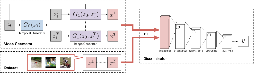
Based on the above discussion, in this paper, we extend an existing GAN model and propose Temporal Generative Adversarial Net (TGAN) that is capable of learning representation from an unlabeled video dataset and producing a new video. Unlike the existing video generator that generates videos with 3D deconvolutional layers [44], in our proposed model the generator consists of two sub networks called a temporal generator and an image generator (Fig.1). Specifically, the temporal generator first yields a set of latent variables, each of which corresponds to a latent variable for the image generator. Then, the image generator transforms these latent variables into a video which has the same number of frames as the variables. The model comprised of the temporal and image generators can not only enable to efficiently capture the time series, but also be easily extended to frame interpolation.
The typical problem that arises from such advanced networks is the instability of training of GANs. In this paper we adopt a recently proposed Wasserstein GAN (WGAN) which tackles the instability, however, we observed that our model still has sensitivity to a hyperparameter of WGAN. Therefore, to deal with this problem, we propose a novel method to remove the sensitive hyperparameter from WGAN and stabilize the training further. The experiments show that our method is more stable than the conventional methods, and the model can be successfully trained even under the situation where the loss diverges with the conventional methods.
Our contributions are summarized as follows. (i) The generative model that can efficiently capture the latent space of the time dimension in videos. It also enables a natural extension to an application such as frame interpolation. (ii) The alternative parameter clipping method for WGAN that significantly stabilizes the training of the networks that have advanced structure.
2 Related work
2.1 Natural image generation
Supervised learning with Convolutional Neural Networks (CNNs) has recently shown outstanding performance in many tasks such as image classification [8, 9, 11] and action recognition [14, 16, 33, 43], whereas unsupervised learning with CNN has received relatively less attention. A common approach for generating images is the use of undirected graphical models such as Boltzmann machines [31, 18, 4]. However, due to the difficulty of approximating gradients, it has been empirically observed that such deep graphical models frequently fail to find good representation of natural images with sufficient diversity. Both Gregor et al. [7] and Dosvotiskiy et al. [3] have proposed models that respectively use recurrent and deconvolutional networks, and successfully generated natural images. However, both models make use of supervised learning and require additional information such as labels.
The Generative Adversarial Network (GAN), which we have mainly employed in this study, is a model for unsupervised learning that finds a good representation of samples by simultaneously training two different networks called the generator and the discriminator. Recently, many extensions for GANs have been proposed. Conditional GANs performs modeling of object attributes [22, 12]. Pathak et al. [26] adopted the adversarial network to generate the contents of an image region conditioned on its surroundings. Li and Wand [19] employed the GAN model in order to efficiently synthesize texture. Denton et al. [2] proposed a Laplacian GAN that outputs a high-resolution image by iteratively generating images in a coarse-to-fine manner. Arjovsky et al. [1] transformed the training of GAN into the minimization problem of Earth Mover’s distance, and proposed a more robust method to train both the generator and the discriminator. Radford et al. [27] also proposed a simple yet powerful model called Deep Convolutional GAN (DCGAN) for generating realistic images with a pair of convolutional and deconvolutional networks. Based on these results, Wang et al. [49] extended DCGAN by factorizing the image generating process into two paths, and proposed a new model called a Style and Structure GAN (-GAN) that exploits two types of generators.
2.2 Video recognition and unsupervised learning
As recognizing videos is a challenging task which has received a lot of attention, many researchers have tackled this problem in various ways. In supervised learning of videos, while a common approach is to use dense trajectories [45, 30, 29], recent methods have employed CNN and achieved state-of-the-art results [14, 16, 33, 43, 24, 46, 47]. Some studies are focused on extracting spatio-temporal feature vectors from a video in an unsupervised manner. Taylor et al. [39] proposed a method that extracts invariant features with Restricted Boltzmann Machines (RBMs). Temporal RBMs have also been proposed to explicitly capture the temporal correlations in videos [40, 38, 37]. Stavens and Thrun [36] dealt with this problem by using an optical flow and low-level features such as SIFT. Le et al. [17] use Independent Subspace Analysis (ISA) to extract spatio-temporal semantic features. Deep neural networks have also been applied to feature extraction from videos [51, 6, 48] in the same way as supervised learning.
There also exist several studies focusing on predicting video sequences from an input sequence with Recurrent Neural Networks (RNNs) represented by Long Short-Term Memory (LSTM) [10]. In particular, Ranzato et al. [28] proposed a Recurrent Neural Network (RNN) model that can learn both spatial and temporal correlations. Srivastava et al. [35] also applied LSTMs and succeeded to predict the future sequence of a simple video. Zhou and Berg [50] proposed a network that creates depictions of objects at future times with LSTMs and DCGAN. Kalchbrenner et al. [15] also employed a convolutional LSTM model, and proposed Video Pixel Networks that directly learn the joint distribution of the raw pixel values. Oh et al. [25] proposed a deep auto-encoder model conditioned on actions, and predicted next sequences of Atari games from a single screen shot and an action sent by a game pad. In order to deal with the problem that generated sequences are “blurry” compared to natural images, Mithieu et al. [21] replaced a standard mean squared error loss and improved the quality of predicted images. However, the above studies cannot directly be applied to the task of generating entire sequences from scratch since they require an initial sequence as an input.
Vondrick et al. [44] recently proposed a generative model that yields a video sequence from scratch with DCGAN consisting of 3D deconvolutional layers. The main difference between their model and ours is model representation; while they simplified the video generation problem by assuming that a background in a video sequence is always static and generate the video with 3D deconvolutions, we do not use such assumption and decompose the generating process of video into the 1D and 2D deconvolutions.
3 Temporal Generative Adversarial Nets
3.1 Generative Adversarial Nets
Before we go into the details of TGAN, we briefly explain the existing GAN [5] and the Wasserstein GAN [1]. A GAN exploits two networks called the generator and the discriminator. The generator is a function that generates samples which looks similar to a sample in the given dataset. The input is a latent variable , where is randomly drawn from a given distribution , e.g., a uniform distribution. The discriminator is a classifier that discriminates whether a given sample is from the dataset or generated by .
The GAN simultaneously trains the two networks by playing a non-cooperative game; the generator wins if it generates an image that the discriminator misclassifies, whereas the discriminator wins if it correctly classifies the input samples. Such minimax game can be represented as
| (1) |
where and are the parameters of the generator and the discriminator, respectively. denotes the empirical data distribution.
3.2 Wasserstein GAN
It is known that the GAN training is unstable and requires careful adjustment of the parameters. To overcome such instability of learning, Arjovsky et al. [1] focused on the property that the GAN training can also be interpreted as the minimization of the Jensen-Shannon (JS) divergence, and proposed Wasserstein GAN (WGAN) that trains the generator and the discriminator to minimize an Earth Mover’s distance (EMD, a.k.a. first Wasserstein distance) instead of the JS divergence. Several experiments the authors conducted reported that WGANs are more robust than ordinal GANs, and tend to avoid mode dropping.
The significant property in the learning of WGAN is “-Lipschitz” constraint with regard to the discriminator. Specifically, if the discriminator satisfies the -Lipschitz constraint, i.e., for all and , the minimax game of WGAN can be represented as
| (2) |
Note that unlike the original GAN, the return value of in Eq.(2) is an unbounded real value, i.e., . In this study we use Eq.(2) for training instead of Eq.(1).
In order to make the discriminator be the -Lipschitz, the authors proposed a method that clamps all the weights in the discriminator to a fixed box denoted as . Although this weight clipping is a simple and assures the discriminator satisfies the -Lipschitz condition, it also implies we cannot know the relation of the parameters between and . As it is known that the objective of the discriminator of Eq.(2) is a good approximate expression of EMD in the case of , this could be a problem when we want to find the approximate value of EMD.
3.3 Temporal GAN
Here we introduce the proposed model based on the above discussion. Let be the number of frames to be generated, and be the temporal generator that gets another latent variable as an argument and generates latent variables denoted as . In our model, is randomly drawn from a distribution .
Next, we introduce image generator that yields a video from these latent variables. Note that takes both the latent variables generated from as well as original latent variable as arguments. While varies with time, is invariable regardless of the time, and we empirically observed that it has a significant role in suppressing a sudden change of the action of the generated video. That is, in our representation, the generated video is represented as .
Using these notations, Eq.(2) can be rewritten as
| (3) |
where is the -th frame of a video in a dataset, and is the latent variable corresponding to -th frame generated by . , , and represent the parameter of , , and , respectively.
3.4 Network configuration
| Temporal generator | Image generator | |
|---|---|---|
| deconv (1, 512, 0, 1) | linear () | linear () |
| deconv (4, 256, 1, 2) | concat + deconv (4, 256, 1, 2) | |
| deconv (4, 128, 1, 2) | deconv (4, 128, 1, 2) | |
| deconv (4, 128, 1, 2) | deconv (4, 64, 1, 2) | |
| deconv (4, 100, 1, 2) | deconv (4, 32, 1, 2) | |
| tanh | deconv (3, 3, 1, 1) + tanh | |
This subsection describes the configuration of our three networks: the temporal generator, the image generator, and the discriminator. Table 1 shows a typical network setting.
Temporal generator
Unlike typical CNNs that perform two-dimensional convolutions in the spatial direction, the deconvolutional layers in the temporal generator perform a one-dimensional deconvolution in the temporal direction. For convenience of computation, we first regard as a one-dimensional activation map of , where the length and the number of channels are one and , respectively. A uniform distribution is used to sample . Next, applying the deconvolutional layers we expand its length while reducing the number of channels. The settings for the deconvolutional layers are the same as those of the image generator except for the number of channels and one-dimensional deconvolution. Like the original image generator we insert a Batch Normalization (BN) layer [13] after deconvolution and use Rectified Linear Units (ReLU) [23] as activation functions.
Image generator
The image generator takes two latent variables as arguments. After performing a linear transformation on each variable, we reshape them into the form shown in Table 1, concatenate them and perform five deconvolutions. These settings are almost the same as the existing DCGAN, i.e., we used ReLU [23] and Batch Normalization layer [13]. The kernel size, stride, and padding are respectively 4, 2, and 2 except for the last deconvolutional layer. Note that the number of output channels of the last deconvolutional layer depends on whether the dataset contains color information or not.
Discriminator
We employ spatio-temporal 3D convolutional layers to model the discriminator. The layer settings are similar to the image generator. Specifically, we use four convolutional layers with kernel and a stride of 2. The number of output channels is 64 in the initial convolutional layer, and set to double when the layer goes deeper. As with the DCGAN, we used LeakyReLU [20] with and Batch Normalization layer [13] after these convolutions. Note that we do not insert the batch normalization after the initial convolution. Finally, we use a fully-connected layer and summarize all of the units in a single scalar. Each shape of the tensor used in the discriminator is shown in Fig.1.
4 Singular Value Clipping
As we described before, WGAN requires the discriminator to fulfill the -Lipschitz constraint, and the authors employed a parameter clipping method that clamps the weights in the discriminator to . However, we empirically observed that the tuning of hyper parameter is severe, and it frequently fails in learning under a different situation like our proposed model. We assumed this problem would be caused by a property that the -Lipschitz constraint widely varies depending the value of , and propose an alternative method that can explicitly adjust the value of .
Suppose that is a composite function consisting of primitive functions, and each function is Lipschitz continuous with . In this case can be represented as , and is also Lipschitz continuous with . That is, what is important in our approach is to add constraints to all the functions such that satisfies the condition of given . Although in principle our method can derive operations that satisfy arbitrary , in the case of these operations are invariant regardless of the number of layers constituting the discriminator. For simplicity we focus on the case of .
| Layer | Condition | Method |
|---|---|---|
| Linear | SVC | |
| Convolution | SVC | |
| Batch normalization | Clipping | |
| LeakyReLU | Do nothing |
To satisfy -Lipschitz constraint, we add a constraint to all linear layers in the discriminator that satisfies the spectral norm of weight parameter is equal or less than one. This means that the singular values of weight matrix are all one or less. To this end, we perform singular value decomposition (SVD) after parameter update, replace all the singular values larger than one with one, and reconstruct the parameters with them. We also apply the same operation to convolutional layers by interpreting a higher order tensor in weight parameter as a matrix . We call these operations Singular Value Clipping (SVC).
As with the linear and the convolutional layer, we clamp the value of which represents a scaling parameter of the batch normalization layer in the same way. We summarize a clipping method of each layer in Table 2. Note that we do not perform any operations on ReLU and LeakyReLU layers because they always satisfy the condition unless in the LeakyReLU is lower than 1.
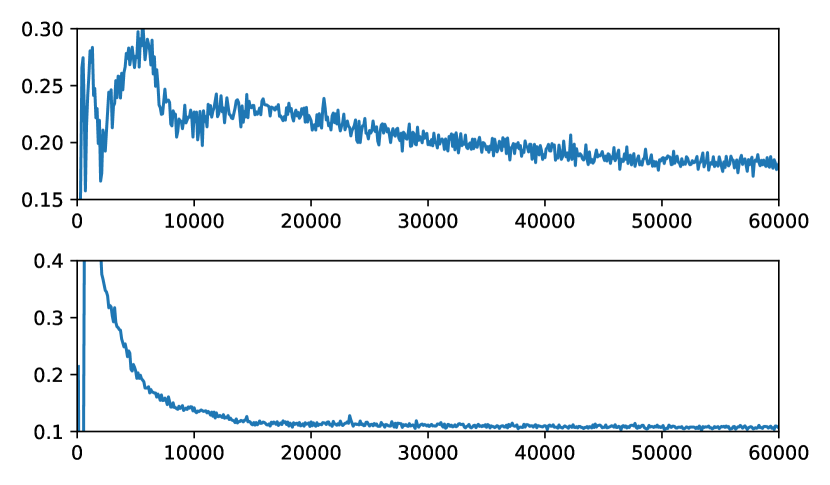
The clear advantage of our alternative clipping method is that it does not require the careful tuning of hyperparameter . Another advantage we have empirically observed is to stabilize the training of WGAN; in our experiments, our method can successfully train an advanced model even under the situation where the behavior of loss function becomes unstable with the conventional clipping. We show an example of such differences in Fig.2.
Although the problem of SVC is an increased computational cost, it can be mitigated by decreasing the frequency of performing the SVC. We show the summary of the algorithm of WGAN with the SVC in Algorithm 1. In our experiments, the computational time of SVD is almost the same as that of the forward-backward computation, but we observed the frequency of clipping is sufficient once every five iterations, i.e., .
5 Applications
5.1 Frame interpolation
One of the advantages of our model is to be able to generate an intermediate frame between two adjacent frames. Since the video generation in our model is formulated as generating a trajectory in the latent image space represented by and , our generator can easily yield long sequences by just interpolating the trajectory. Specifically, we add a bilinear filter to the last layer of the temporal generator, and interpolate the trajectory in the latent image space (see Section 1).
5.2 Conditional TGAN
In some cases, videos in a dataset contain some labels which correspond to a category of the video such as “IceDancing” or “Baseball”. In order to exploit them and improve the quality of videos by the generator, we also develop a Conditional TGAN (CTGAN), in which the generator can take both label and latent variable .
The structure of CTGAN is similar with that of the original Conditional GAN. In temporal generator, after transforming into one-hot vector , we concatenate both this vector and , and regard it as a new latent variable. That is, the temporal generator of the CTGAN is denoted as . The image generator of the CTGAN also takes the one-hot label vector as arguments, i.e., . As with the original image generator, we first perform linear transformation on each variable, reshape them, and operate five deconvolutions.
In the discriminator, we first broadcast the one-hot label vector to a voxel whose resolution is the same as that of the video. Thus, if the number of elements of is , the number of channels of the voxel is equal to . Next, we concatenate both the voxel and the input video, and send it into the convolutional layers.
6 Experiments
6.1 Datasets
We performed experiments with the following datasets.
Moving MNIST
To investigate the properties of our models, we trained the models on the moving MNIST dataset [35], in which there are 10,000 clips each of which has 20 frames and consists of two digits moving inside a patch. In these clips, two digits move linearly and the direction and magnitude of motion vectors are randomly chosen. If a digit approaches one of the edges in the patch, it bounces off the edge and its direction is changed while maintaining the speed. In our experiments, we randomly extracted frames from these clips and used them as a training dataset.
UCF-101
UCF-101 is a commonly used video dataset that consists of 13,320 videos belonging to 101 different categories such as IceDancing and Baseball Pitch [34]. Since the resolution of videos in the dataset is too large for the generative models, we resized all the videos to pixels, randomly extracted 16 frames, and cropped a center square with 64 pixels.
Golf scene dataset
Golf scene dataset is a large-scale video dataset made by Vondrick et al. [44], and contains 20,268 golf videos with resolution. Since each video includes 29 short clips on average, it contains 583,508 short video clips in total. As with the UCF-101, we resized all the video clips with pixels. To satisfy the assumption that the background is always fixed, they stabilized all of the videos with SIFT and RANSAC algorithms. As such assumption is not included in our method, this dataset is considered to be advantageous for existing methods.
6.2 Training configuration
All the parameters used in the optimizer are the same as those of the original WGAN. Specifically, we used the RMSProp optimizer [41] with the learning rate of . All the weights in the temporal generator and the discriminator are initialized with HeNormal [8], and the weights in the image generator are initialized with the uniform distribution within a range of . Chainer [42] was used to implement all models and for experiments.
For comparison, we employed the conventional clipping method and the SVC to train models with the WGAN. In the conventional clipping method, we carefully searched clipping parameter and confirmed that the best value is . We set to 1 for the both methods.
6.3 Comparative methods
For comparison, we implemented two models: (i) a simple model in which the generator has one linear layer and four 3D deconvolutional layers and the discriminator has five 3D convolutional layers, and (ii) a Video GAN proposed by [44]. We call the former “3D model”. In the generator of the 3D model, all the deconvolutional layers have kernel and the stride of 2. The number of channels in the initial deconvolutional layer is 512 and set to half when the layer goes deeper. We also used ReLU and batch normalization layers. The settings of the discriminator are exactly the same as those of our model. In the settings of the video GAN, we simply followed the settings in the original paper.
When we tried to train the 3D model and the video GAN model with the normal GAN loss, we observed that the discriminator easily wins against the generator and the training cannot proceed. To avoid this, we added Gaussian noise () to all layers of discriminators. In this case, all the scale parameters after the Batch Normalization layer are not used. Note that this noise addition is not used when we use the WGAN.
6.4 Qualitative evaluation
We trained our proposed model on the above datasets and visually confirmed the quality of the results. Fig.3 shows examples of generated videos by the generator trained on the moving MNIST dataset. It can be seen that the generated frames are quite different from those of the existing model proposed by Srivastava et al. [35]. While the predicted frames by the existing model tend to be blurry, our model is capable of producing consistent frames in which each image is sharp, clear and easy to discriminate two digits. We also observed that although our method can generate the frames in which each digit continues to move in a straight line, its shape sometimes slightly changes by time. Note that the existing models such as [35, 15] seem to generate frames in which each digit does not change, however, these methods can not be directly compared with our method because the qualitative results the authors have shown are for “video prediction” that predicts future frames from initial inputs, whereas our method generates them without such priors.
Fig.3 also shows that as for the quality of the generated videos, the 3D model using the normal GAN is the worst compared with the other methods. We considered that it is due to the high degree of freedom in the model caused by three-dimensional convolution, and explicitly dividing the spatio-temporal space could contribute to the improvement of the quality. We also confirmed that it is not the effect of selecting the normal GAN; although the quality of samples generated by the 3D model with the SVC outperforms that of the 3D model with the normal GAN, it is still lower than our proposed model (model (d) in Fig.3). In order to illustrate the effectiveness of in , we further conducted the experiment with the TGAN in which does not take as an argument (model (c)). In this experiment, we observed that in the model (c) the problem of mode collapse tends to occur compared to our model.
We also compared the performance of our method with other existing methods when using practical data sets such as UCF-101. The qualitative experimental results are shown in Fig.4. We observed that the videos generated by the 3D model have the most artifacts compared with other models. The video GAN tends to avoid these artifacts because the background is relatively fixed in the UCF-101, however, the probability of generating unidentified videos is higher than that of the proposed model. We inferred that this problem is mainly due to the weakness of the existing method is vulnerable to videos with background movement.
Finally, in order to indicate that the quality of our model is comparable with that of the video GAN (these results can be seen in their project page), we conducted the experiment with the golf scene dataset. As we described before, it is considered that this dataset, in which the background is always fixed, is advantageous for the video GAN that exploits this assumption. Even under such unfavorable conditions, the quality of the videos generated by our model is almost the same as the existing method; both create a figure that seems likes a person’s shadow, and it changes with time.
6.4.1 Applications
We performed the following experiments to illustrate the effectiveness of the applications described in Section 5.
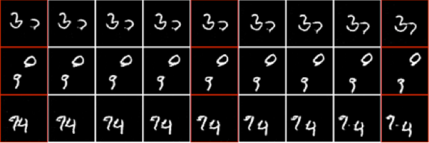
To show our model can be applied to frame interpolation, we generated intermediate frames by interpolating two adjacent latent variables of the image space. These results are shown in Fig.6. It can be seen that the frame is not generated by a simple interpolation algorithm like dissolve, but semantically interpolating the adjacent frames.
We also experimentally confirmed that the proposed model is also extensible to the conditional GAN. These results are shown in Fig.7. We observed that the quality of the video generated by the conditional TGAN is significantly higher than that of the unsupervised ones. It is considered that adding semantic information of labels to the model contributed to the improvement of quality.
6.5 Quantitative evaluation
| Model A | Model B | GAM score | Winner |
|---|---|---|---|
| TGAN | 3D model (GAN) | TGAN | |
| TGAN | 3D model (SVC) | TGAN | |
| TGAN | TGAN () | TGAN |
We performed the quantitative experiment to confirm the effectiveness of our method. As indicators of the quantitative evaluation, we adopted a Generative Adversarial Metric (GAM) [12] that compares adversarial models against each other, and an inception score [32] that has been commonly used to measure the quality of the generator.
For the comparison of two generative models, we used GAM scores in the moving MNIST dataset. Unlike the normal GAN in which the discriminator uses the binary cross entropy loss, the discriminator of the WGAN is learned to keep the fake samples and the real samples away, and we cannot choose zero as a threshold for discriminating real and fake samples. Therefore, we first generate a sufficient number of fake samples, and set a score that can classify fake and real samples well as the threshold.
Table 3 shows the results. In the GAM, a score higher than one means that the model A generates better fake samples that can fool the discriminator in the model B. It can be seen that our model can generate better samples that can deceive other existing methods. It can be seen that the TGAN beats the 3D models easily, but wins against the TGAN in which has only. These results are the same as the results obtained by the aforementioned qualitative evaluation.
In order to compute the inception score, a dataset having label information and a good classifier for identifying the label are required. Thus, we used the UCF-101 dataset that has 101 action categories, and a pre-trained model of C3D [43], which was trained on Sports-1M dataset [16] and fine-tuned for the UCF-101, was employed as a classifier. We also calculated the inception scores by sampling 10,000 times from the latent random variable, and derived rough standard deviation by repeating this procedure four times. To compute the inception score when using the conditional TGAN, we added the prior distribution for the category to the generator, and transformed the conditional generator into the generator representing the model distribution. We also computed the inception score when using a real dataset to see an upper bound.
| Method | Inception score |
|---|---|
| 3D model (Weight clipping) | |
| 3D model (SVC) | |
| Video GAN [44] (Normal GAN) | |
| Video GAN (SVC) | |
| TGAN (Normal GAN) | |
| TGAN (Weight clipping) | |
| TGAN (SVC) | |
| Conditional TGAN (SVC) | |
| UCF-101 dataset |
Table 4 shows quantitative results. It can be seen that in the 3D model, the quality of the generated videos is worse than the video GAN and our proposed model. Although we observed that using the SVC slightly improves the inception score, its value is a little and still lower than that of the video GAN. We also confirmed that the SVC is effective in the case of the video GAN, however, its value is lower than our models. On the other hand, our models achieve the best scores compared with other existing methods. In addition to the video GAN, the TGAN using the SVC slightly outperformed the TGAN using the conventional weight clipping method. Although the quality of the SVC is almost indistinguishable compared with existing methods, we had to carefully change the value of to achieve such quality. We believe that our clipping method is not a tool for dramatically improving the quality of the generator, but a convenient method to reduce the trouble of adjusting hyper parameters and significantly stabilize the training of the models.
7 Summary
We proposed a generative model that learns semantic representation of videos and can generate image sequences. We formulated the generating process of videos as a series of (i) a function that generates a set of latent variables, and (ii) a function that converts them into an image sequence. Using this representation, our model can generate videos with better quality and naturally achieves frame interpolation. We also proposed a novel parameter clipping method, Singular Value Clipping (SVC), that stabilizes the training of WGAN.
Acknowledgements
We would like to thank Brian Vogel, Jethro Tan, Tommi Kerola, and Zornitsa Kostadinova for helpful discussions.
References
- [1] M. Arjovsky, S. Chintala, and L. Bottou. Wasserstein GAN. In arXiv preprint arXiv:1701.07875, 2017.
- [2] E. Denton, S. Chintala, A. Szlam, and R. Fergus. Deep Generative Image Models Using a Laplacian Pyramid of Adversarial Networks. In NIPS, 2015.
- [3] A. Dosovitskiy, J. T. Springenberg, M. Tatarchenko, and T. Brox. Learning to Generate Chairs, Tables and Cars with Convolutional Networks. arXiv preprint arXiv:1411.5928, 2014.
- [4] S. M. A. Eslami, N. Heess, and J. Winn. The Shape Boltzmann Machine : a Strong Model of Object Shape. In CVPR, 2012.
- [5] I. J. Goodfellow, J. Pouget-Abadie, M. Mirza, B. Xu, D. Warde-Farley, S. Ozair, A. Courville, and Y. Bengio. Generative Adversarial Nets. In NIPS, 2014.
- [6] R. Goroshin, J. Bruna, J. Tompson, D. Eigen, and Y. LeCun. Unsupervised Learning of Spatiotemporally Coherent Metrics. In ICCV, 2015.
- [7] K. Gregor, I. Danihelka, A. Graves, D. J. Rezende, and D. Wierstra. DRAW: A Recurrent Neural Network For Image Generation. arXiv preprint arXiv:1502.04623, 2015.
- [8] K. He, X. Zhang, S. Ren, and J. Sun. Delving Deep into Rectifiers: Surpassing Human-Level Performance on ImageNet Classification. ICCV, 2015.
- [9] K. He, X. Zhang, S. Ren, and J. Sun. Deep Residual Learning for Image Recognition. In CVPR, 2016.
- [10] S. Hochreiter and J. Schmidhuber. Long short-term memory. Neural Computation, 9(8):1735—-1780, 1997.
- [11] G. Huang, Z. Liu, and K. Q. Weinberger. Densely Connected Convolutional Networks. In arXiv preprint arXiv:1608.06993, 2016.
- [12] D. J. Im, C. D. Kim, H. Jiang, and R. Memisevic. Generating images with recurrent adversarial networks. In arXiv preprint arXiv:1602.05110, 2016.
- [13] S. Ioffe and C. Szegedy. Batch Normalization: Accelerating Deep Network Training by Reducing Internal Covariate Shift. arXiv preprint arXiv:1502.03167, 2015.
- [14] S. Ji, W. Xu, M. Yang, and K. Yu. 3D Convolutional Neural Networks for Human Action Recognition. PAMI, 35(1):221–231, jan 2013.
- [15] N. Kalchbrenner, A. van den Oord, K. Simonyan, I. Danihelka, O. Vinyals, A. Graves, and K. Kavukcuoglu. Video Pixel Networks. In arxiv preprint arXiv:1610.00527, 2016.
- [16] A. Karpathy, S. Shetty, G. Toderici, R. Sukthankar, T. Leung, and Li Fei-Fei. Large-scale Video Classification with Convolutional Neural Networks. In CVPR, 2014.
- [17] Q. V. Le, W. Y. Zou, S. Y. Yeung, and A. Y. Ng. Learning hierarchical invariant spatio-temporal features for action recognition with independent subspace analysis. In CVPR, 2011.
- [18] H. Lee, R. Grosse, R. Ranganath, and A. Y. Ng. Convolutional Deep Belief Networks for Scalable Unsupervised Learning of Hierarchical Representations. In ICML. ACM Press, 2009.
- [19] C. Li and M. Wand. Precomputed Real-Time Texture Synthesis with Markovian Generative Adversarial Networks. In arxiv preprint arXiv:1604.04382, 2016.
- [20] A. L. Maas, A. Y. Hannun, and A. Y. Ng. Rectifier Nonlinearities Improve Neural Network Acoustic Models. In ICML, 2013.
- [21] M. Mathieu, C. Couprie, and Y. LeCun. Deep Multi-Scale Video Prediction beyond Mean Square Error. In ICLR, 2016.
- [22] M. Mirza and S. Osindero. Conditional Generative Adversarial Nets. arXiv preprint arXiv:1411.1784, 2014.
- [23] V. Nair and G. E. Hinton. Rectified Linear Units Improve Restricted Boltzmann Machines. ICML, (3):807–814, 2010.
- [24] J. Y.-H. Ng, M. Hausknecht, S. Vijayanarasimhan, O. Vinyals, R. Monga, and G. Toderici. Beyond Short Snippets: Deep Networks for Video Classification. In CVPR, 2015.
- [25] J. Oh, X. Guo, H. Lee, R. Lewis, and S. Singh. Action-Conditional Video Prediction using Deep Networks in Atari Games. In NIPS, 2015.
- [26] D. Pathak, P. Krähenbühl, J. Donahue, T. Darrell, and A. A. Efros. Context Encoders: Feature Learning by Inpainting. In CVPR, 2016.
- [27] A. Radford, L. Metz, and S. Chintala. Unsupervised Representation Learning with Deep Convolutional Generative Adversarial Networks. In ICLR, 2016.
- [28] M. Ranzato, A. Szlam, J. Bruna, M. Mathieu, R. Collobert, and S. Chopra. Video (language) modeling: a baseline for generative models of natural videos. arXiv preprint arXiv:1412.6604, 2014.
- [29] M. Rohrbach, S. Amin, M. Andriluka, and B. Schiele. A Database for Fine Grained Activity Detection of Cooking Activities. In CVPR, 2012.
- [30] S. Sadanand and J. J. Corso. Action Bank: A High-Level Representation of Activity in Video. In CVPR, 2012.
- [31] R. Salakhutdinov and G. Hinton. Deep Boltzmann Machines. In AISTATS, 2009.
- [32] T. Salimans, I. Goodfellow, W. Zaremba, V. Cheung, A. Radford, and X. Chen. Improved Techniques for Training GANs. In NIPS, 2016.
- [33] K. Simonyan and A. Zisserman. Two-Stream Convolutional Networks for Action Recognition in Videos. In NIPS, 2014.
- [34] K. Soomro, A. R. Zamir, and M. Shah. UCF101: A Dataset of 101 Human Actions Classes From Videos in The Wild. arXiv preprint arXiv:1212.0402, 2012.
- [35] N. Srivastava, E. Mansimov, and R. Salakhutdinov. Unsupervised Learning of Video Representations using LSTMs. In ICML, 2015.
- [36] D. Stavens and S. Thrun. Unsupervised Learning of Invariant Features Using Video. In CVPR, 2010.
- [37] I. Sutskever, G. Hinton, and G. Taylor. The Recurrent Temporal Restricted Boltzmann Machine. In NIPS, 2009.
- [38] I. Sutskever and G. E. Hinton. Learning Multilevel Distributed Representations for High-Dimensional Sequences. In AISTATS, 2007.
- [39] G. W. Taylor, R. Fergus, Y. LeCun, and C. Bregler. Convolutional Learning of Spatio-temporal Features. In ECCV, 2010.
- [40] G. W. Taylor, G. E. Hinton, and S. Roweis. Modeling Human Motion Using Binary Latent Variables. In NIPS, 2007.
- [41] T. Tieleman and G. Hinton. Lecture 6.5 - RmsProp: Divide the gradient by a running average of its recent magnitude. COURSERA: Neural Networks for Machine Learning, 2012.
- [42] S. Tokui, K. Oono, S. Hido, and J. Clayton. Chainer: a Next-Generation Open Source Framework for Deep Learning. In Proceedings of Workshop on Machine Learning Systems in NIPS, 2015.
- [43] D. Tran, L. Bourdev, R. Fergus, L. Torresani, and M. Paluri. Learning Spatiotemporal Features with 3D Convolutional Networks. In ICCV, 2015.
- [44] C. Vondrick, H. Pirsiavash, and A. Torralba. Generating Videos with Scene Dynamics. In NIPS, 2016.
- [45] H. Wang, A. Kl¨aser, C. Schmid, and L. Cheng-Lin. Action Recognition by Dense Trajectories. In CVPR, 2011.
- [46] L. Wang, Y. Qiao, and X. Tang. Action Recognition with Trajectory-Pooled Deep-Convolutional Descriptors. In CVPR, 2015.
- [47] L. Wang, Y. Xiong, Z. Wang, Y. Qiao, D. Lin, X. Tang, and L. V. Gool. Temporal Segment Networks: Towards Good Practices for Deep Action Recognition. In ECCV, 2016.
- [48] X. Wang and A. Gupta. Unsupervised Learning of Visual Representations using Videos. In ICCV, 2015.
- [49] X. Wang and A. Gupta. Generative Image Modeling using Style and Structure Adversarial Networks. arXiv preprint arXiv:1603.05631, 2016.
- [50] Y. Zhou and T. L. Berg. Learning Temporal Transformations From Time-Lapse Videos. In ECCV, 2016.
- [51] W. Y. Zou, S. Zhu, A. Y. Ng, and K. Yu. Deep Learning of Invariant Features via Simulated Fixations in Video. In NIPS, 2012.