FURL: Fixed-memory and Uncertainty Reducing Local Triangle Counting for Graph Streams

Abstract

How can we accurately estimate local triangles for all nodes in simple and multigraph streams? Local triangle counting in a graph stream is one of the most fundamental tasks in graph mining with important applications including anomaly detection and social network analysis. Although there have been several local triangle counting methods in a graph stream, their estimation has a large variance which results in low accuracy, and they do not consider multigraph streams which have duplicate edges. In this paper, we propose Furl, an accurate local triangle counting method for simple and multigraph streams. Furl improves the accuracy by reducing a variance through biased estimation and handles duplicate edges for multigraph streams. Also, Furl handles a stream of any size by using a fixed amount of memory. Experimental results show that Furl outperforms the state-of-the-art method in accuracy and performs well in multigraph streams. In addition, we report interesting patterns discovered from real graphs by Furl, which include unusual local structures in a user communication network and a core-periphery structure in the Web.

1 Introduction

How can we accurately estimate local triangles for all nodes in simple and multigraph streams? The local triangle counting problem is to count the number of triangles containing each node in a graph, and has been extensively studied because of its wide and important applications. For instance, it has been used for social role identification of a user WelserGFS07 ; chou2010discovering , content quality evaluation BecchettiBCG10 , data-driven anomaly detection BecchettiBCG10 ; YangWWGZD11 ; LimK15 , community detection BerryHLP11 ; suri2011counting , motif detection MilEtAl02 , clustering ego-networks epasto2015ego , and uncovering hidden thematic layers EckmannM02 .

Although a number of local triangle counting methods have been successfully applied to graph streams, there are two challenging issues. First, their large variance causes low accuracy. In a graph stream model where edges continuously arrive, only one trial is allowed and a large variance causes large difference between estimated and true local triangle counts. Thus previous local triangle counting methods do not produce stable results and show bad worst case performance. Second, recent real world graph streams contain duplicate edges, i.e., they are multigraph streams. Examples include a communication network in Internet, a phone call history, SNS messages like tweets, an email network, etc. In such environments it is crucial to carefully handle duplicate edges in local triangle counting.

In this paper, we propose Furl, an accurate local triangle counting method for simple and multigraph streams. Furl guarantees the fixed amount of memory usage, regardless of the size of a graph stream. Furl has two main versions: Furl-SX and Furl-MX for simple and multigraph streams, respectively. Furl-SX improves the accuracy of the previous state-of-the-art by reducing a variance through biased estimation. Furl-MX, the first algorithm for local triangle counting in multigraph streams, carefully handles multigraph streams by using reservoir sampling with random hash to sample distinct items uniformly at random, and reduces a variance of estimation.

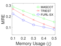
(a) Youtube

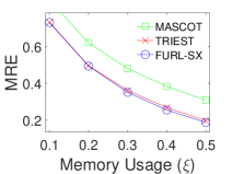
(b) Pokec

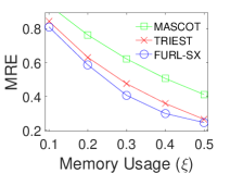
(c) Skitter

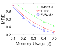
(d) Hudong

Figure 1: Mean of relative error (MRE) vs. memory usage of Furl-SX and two competing methods Mascot and Triest for local triangle counting in simple graph stream. We choose 0.7, 0.1, 0.4, and 0.4 as $\delta$ in Youtube, Pokec, Skitter, and Hudong, respectively. Furl-SX gives the minimum error for a given memory usage.

Our contributions are summarized as follows.

Algorithm. We propose Furl, an accurate local triangle counting algorithm for simple and multigraph streams. Furl uses a fixed amount of memory, and thus it can handle streams of any sizes. Furl improves the accuracy of previous simple graph stream algorithms by decreasing variance; furthermore, Furl handles multigraph streams by carefully updating triangle counts. We give theoretical results on the accuracy bound of Furl.

Performance. We demonstrate that Furl-SX, a version of Furl for simple graph stream, outperforms the state-of-the-art method as shown in Figure 1. We also show that Furl-MX, a version of Furl for multigraph stream, performs well in multigraph streams.

Discovery. We present interesting patterns discovered by applying Furl to large real graph data, which include egonetworks forming a near clique/star in a user communication network, and a core-periphery structure in the Web.

The code and datasets used in the paper are available in http://datalab.snu.ac.kr/furl. The rest of this paper is organized as follows. Section 2 gives related works and preliminaries. Section 3 describes our proposed method Furl. In Section 4, we evaluate the performance of Furl and give discovery results. We conclude in Section 5. Table 1 shows the symbols used in this paper.

Table 1: Table of symbols.

Symbol	Description
$S$	Graph stream
$V,E$	Set of nodes and edges
$u,v,w$	Nodes
$e$	Edges
$N_{u}$	Set of neighbors of $u$
$N_{uv}$	Set of common neighbors of $u$ and $v$
$n,m$	Number of nodes and edges
$O_{e}$	Number of occurence of an edge $e$ in multigraph stream
$u(T)$	Number of unique edges in a stream at time $T$
$D$	Buffer
$|D|$	Number of elements stored in buffer $D$
$M$	Buffer size
$h_{max}$	Maximum hash value in a stream
$D_{max}$	Edge whose hash value is $h_{max}$
$B$	Current bucket
$b_{\lambda}$	Bucket that $\lambda$ appears
$J$	Bucket size
$\delta$	Decaying factor for past estimations
$\lambda$	Triangle
$T,t$	Current time, and time
$T_{\lambda}$	Time that a triangle $\lambda$ is counted
$T_{M}$	Last time when local triangle estimation equals the true triangle count
$\varDelta_{u}$	True local triangle count of node $u$
$c_{u}$	Estimated local triangle count of node $u$ in Furl-S and Furl-M
$\tau_{u}$	Estimated local triangle count of node $u$ in Furl-SX and Furl-MX
$q_{\lambda}$	Triangle estimation weight of a triangle $\lambda$
$X_{\lambda}$	Estimated triangle counts by Furl-S and Furl-M
$Y_{\lambda}$	Estimated triangle counts by Furl-SX and Furl-MX

2 Related Works

In this section, we present related works about triangle counting and reservoir sampling in a data stream.

2.1 Global Triangle Counting

There have been works on the counting of the number of triangles. Usually, existing algorithms for global triangle counting are in-memory algorithms, whose performance cannot scale up with massive graphs.

To scale up with massive graphs, various approaches have been proposed. Chu and Cheng ChuC11 developed an I/O-efficient algorithm. Their algorithm avoids random disk access by partitioning the graph into components and processing them in parallel. Hu et al. HuTC13 devised an I/O and CPU efficient algorithm whose I/O complexity is $O(m^{2}/(MB))$, where $m$, $M$ and $B$ are the number of edges, the size of internal memory, and the size of block, respectively. Thereafter, Pagh and Silvestri PaghS14 improved the minimum I/O complexity to $O(m^{3/2}/B\sqrt{M})$ in expectation. Cohen Cohen09 proposed the first MapReduce algorithm. Suri and Vassilvitskii SuriV11 presented a graph partitioning based algorithm for the MapReduce framework. Later, the algorithm is improved by Park and Chung ParkC13 . Recently, there have been more parallel algorithms ArifuzzamanKM13 ; KimHLPY14 ; ParkSKP14 .

There have been considerable studies on triangle counting in a graph stream, beginning with Bar-Yossef et al. Bar-YossefKS02 . After that, Jowhari et al. JowhariG05 improved the space usage. Buriol et al. BuriolFLMS06 designed two algorithms which scale very well in a stream of edges. Each algorithm respectively takes constant and $O(\log(n(1+sn/m)))$ expected update time, where $s$ is the space requirement and $n$ is the number of nodes. Tsourakakis et al. TsourakakisKMF09 proposed a one pass algorithm based on edge sampling to count triangles of a graph. This sampling technique was generalized by AhmedDNK14 for counting arbitrary subgraphs. Jha et al. JhaSP13 presented a space efficient algorithm to estimate the number of total triangles with a single pass to an input graph. Kane et al. KaneMSS12 provided a sketch based streaming algorithm for estimating the number of arbitrary subgraphs with a constant size in a large graph. Afterwards, Pavan et al. PavanTTSW13 made the space and time complexity better. Note that global triangle counting is different from local triangle counting, the focus of this paper, to compute the number of triangles of all individual nodes.

2.2 Local Triangle Counting

For local triangle counting, a simple and fast algorithm is to get $A^{3}$ for an adjacency matrix $A$ AlonYZ97 . It takes only $O(m^{1.41})$ time, but its memory usage, $O(n^{2})$, is quadratic. Latapy Latapy08 presented a fast and space-efficient algorithm, but in a non-stream setting. To handle simple graph streams, Becchetti et al. BecchettiBCG10 devised a semi-streaming algorithm based on min-wise independent permutations BroderCFM98 . Their algorithm requires $O(n)$ space in main memory and $O(\log(n))$ sequential scans over the edges of the graph. However, it is inappropriate for handling a graph stream in real time due to its multiple scans to the graph. Kutzkov and Pagh KutzkovP13 proposed a randomized one pass algorithm based on node coloring PaghT12 . Despite the property of scanning once, it is limited in practice because it requires prior knowledge about the graph. These problems are resolved by Mascot proposed in LimK15 and it is based on a triangle counting method TsourakakisKMF09 which uses an edge sampling. Mascot takes only one parameter of edge sampling probability with one sequential scan to the graph stream but Mascot does not guarantee the memory usage; it means that eventually the out-of-memory error will happen. De Stefani et al. StefaniERU16 proposed Triest which computes the number of triangles in fully-dynamic streams with a fixed memory size. Their large variance, however, causes low accuracy since accuracy heavily depends on a variance in a stream setting. Our proposed algorithm Furl-SX improves the accuracy of Triest by reducing the variance through biased estimation. For multigraph streams, there are no existing works.

2.3 Reservoir Sampling

Reservoir sampling is a technique to sample a given number of elements from a stream uniformly at random Vitter85 . Let $S$ be a stream of items, and $D$ be an array of size $M$. For each item $e$ arriving at time $T\geq 1$, the sampling procedure is as follows. If $T\leq M$, $e$ is unconditionally stored in $D_{T}$, the $T$th item of $D$. If $T>M$, first pick a random integer $i$ from $\{1,\ldots,T\}$. If $i\leq M$, the existing item at $D_{i}$ is dropped and $e$ is stored at $D_{i}$; otherwise, $e$ is discarded. As a result, the sampling probability for every observed item becomes $\min(M/T,1)$ at time $T$. This reservoir sampling is used in our algorithms to keep a constant number of edges from a graph stream regardless of its length, as presented in Section 3.

Reservoir Sampling With Random Hash

Reservoir sampling with random hash (random sort sunter1977list ) is a modification of reservoir sampling to sample distinct items uniformly at random in stream environment. The main idea is to assign each item a random hash value and to keep $M$ items with minimum hash values. The arriving item $e$ is sampled if and only if $h(e)<h_{max}=\max_{f\in D}h(f)$. Note that items in the buffer have minimal hash values among all items in a stream. The sampling technique samples distinct items uniformly at random, because it is equivalent to picking $M$ distinct items with minimum values in the whole stream. The reservoir sampling with random hash is used in Furl-M to process multigraph streams.

3 Proposed Method

How can we accurately estimate local triangles in simple and multigraph streams with a fixed memory space? In this section, we propose Furl, a suite of accurate and memory efficient local triangle counting methods for graph streams to answer the question. We first present two basic algorithms Furl-S (Section 3.1) and Furl-M (Section 3.2) based on the reservoir sampling: Furl-S is an algorithm for simple graph streams, and Furl-M is an algorithm for multigraph streams. Our main proposed algorithms Furl-SX and Furl-MX (Section 3.3) further improve the accuracy of Furl-S and Furl-M by additionally assembling intermediate estimation results. Note that in all the proposed methods, we store edges only in a buffer $D$ which has a fixed capacity $M$.

3.1 FURL for Simple Graph

We present Furl-S (Algorithm 1) which estimates local triangles in simple graph streams without duplicate edges. The algorithm computes triangle estimations with a fixed memory using reservoir sampling, and decouples two events of sampling and counting a triangle for efficiency using the idea of MASCOT LimK15 . A recent method called TRIEST StefaniERU16 , which also uses the same idea of combining MASCOT and the reservoir sampling, has been proposed independently. Below, we describe the procedure of the method.

Let $T$ be the current time, $e=(u,v)$ be a new edge arriving from a stream at time $T$, and $c_{u}$ be local triangles estimation of node $u$. First, local triangle estimation is updated if the new edge $e$ forms a triangle with two edges in the sample graph (lines 1–1). If a triangle $\lambda$ is counted by Furl-S it is when its last edge arrives. Before the buffer $D$ overflows, Furl-S has the exact triangle counts since the buffer stores all edges which have arrived so far. The triangle estimation is increased by factor $1$ when we have the exact triangle counts, and it is increased by factor $q_{T}=\frac{(T-1)(T-2)}{M(M-1)}$ otherwise. $ExactCnt$ in Algorithm 1 indicates whether $c_{u}$ equals the true local triangle count of node $u$ or not, and is initialized to $true$. Let $N_{x}$ and $N_{xy}$ be a set of neighbors of $x$, and a set of common neighbors of $x$ and $y$ in the sample graph, respectively. Then, for each $e=(u,v)$ from the stream, $c_{u}$ and $c_{v}$ increase by $|N_{uv}|\cdot\theta$, and for every $w\in N_{uv}$, $c_{w}$ increases by $\theta$ where $\theta$ is a triangle estimation increase factor. The second task is to sample $e$ with probability $\min(M/T,1)$ using reservoir sampling. In the sampling procedure, $ExactCnt$ turns to $false$ when the buffer overflows (line 1), because $D$ does not store all arriving edges anymore.

1

2

Input: Graph stream $S$, and max. number $M$ of edges to store

Output: Local triangle estimation $c$

3

4

5$G\leftarrow(V,D)$ with $V=D=\emptyset$.

6 $D$ is initialized by $M$ dummy edges.

7 The estimated count $c$ for nodes is initialized to $\emptyset$.

8 The boolean flag $ExactCnt$ is initialized to $true$.

9 foreach edge $e=(u,v)$ from $S$ do   // at time $T$

10       $\textnormal{{$DiscoverNode$}}(u)$.

11       $\textnormal{{$DiscoverNode$}}(v)$.

12       $\textnormal{{$UpdateTriangles\text{-S}$}}(e)$.

13       $\textnormal{{$SampleNewEdge\text{-S}$}}(e)$

14 end foreach

15

16

17Subroutine $DiscoverNode$(u)

18       if $u\notin V$ then $V\leftarrow V\cup\{u\}$ and $c_{u}=0$.

19      

20 end

21

22Subroutine $UpdateTriangles\text{-S}$(e)

23       if $ExactCnt=true$ then  $\textnormal{{$IncreaseEstimation$}}(e,1)$.

24      else

25             $q_{T}\leftarrow\frac{(T-1)(T-2)}{M(M-1)}$.

26             $\textnormal{{$IncreaseEstimation$}}(e,q_{T})$.

27            

28       end if

29      

30 end

31

32Subroutine $IncreaseEstimation$($e=(u,v)$, $\theta$)

33       $N_{uv}\leftarrow N_{u}\cap N_{v}.$

34       foreach $w\in N_{uv}$ do  $c_{w}\leftarrow c_{w}+\theta$.

35       $c_{u}\leftarrow c_{u}+\left(\theta\times|N_{uv}|\right)$.

36       $c_{v}\leftarrow c_{v}+\left(\theta\times|N_{uv}|\right)$.

37      

38 end

39

40Subroutine $SampleNewEdge\text{-S}$(e)

41       if $|D|<M$ then  Append $e$ to D.

42      else

43             if $ExactCnt=true$ then  $ExactCnt\leftarrow false$.

44             $\textnormal{{$ReplaceEdge\text{-S}$}}(e)$.

45            

46       end if

47      

48 end

49

50Subroutine $ReplaceEdge\text{-S}$(e)

51       $i\leftarrow uniform(1,T)$.

52       if $i\leq M$ then  $D_{i}\leftarrow e$

53      

54 end

55

Algorithm 1 Furl-S for simple graph stream

Furl-S provides unbiased estimation as shown in the following Lemma 1. Note that we do not consider when $ExactCnt$ is $true$ since Furl-S provides the exact counting.

Lemma 1

Let $\varDelta_{u}$ be the true local triangle count for a node $u$, and $c_{u}$ be the estimation given by Furl-S. For every node $u$, $\mathbb{E}\left[c_{u}\right]=\varDelta_{u}.$

Proof 1

Let $T_{\lambda}$ be the time $\lambda$ is formed, $S_{\lambda}^{-}$ be a set of triangles that are formed when we have the exact triangle counts, i.e. $T_{\lambda}\leq M+1$ , and $S_{\lambda}^{+}$ be a set of triangles that are formed when we do not have the exact triangle counts, i.e. $T_{\lambda}>M+1$. Note that every triangle is included in either $S_{\lambda}^{-}$ or $S_{\lambda}^{+}$. We define $X_{\lambda}^{-}$ and $X_{\lambda}^{+}$ as follows.

$$X_{\lambda}^{-}=\begin{cases}1&\lambda\ is\ counted\\ 0&otherwise.\end{cases}$$

$$X_{\lambda}^{+}=\begin{cases}q_{T_{\lambda}}=\frac{(T_{\lambda}-1)(T_{\lambda}-2)}{M(M-1)}&\lambda\ is\ counted\\ 0&otherwise.\end{cases}$$

Then,

$$\mathbb{E}\left[c_{u}\right]=\sum\limits_{\lambda\in\Lambda_{u}\cap S_{\lambda}^{-}}\mathbb{E}\left[X_{\lambda}^{-}\right]+\sum\limits_{\lambda\in\Lambda_{u}\cap S_{\lambda}^{+}}\mathbb{E}\left[X_{\lambda}^{+}\right]$$

where $\Lambda_{u}$ is the set of triangles containing $u$. For a triangle $\lambda\in\Lambda_{u}\cap S_{\lambda}^{-}$,

$$\mathbb{E}\left[X_{\lambda}^{-}\right]=1\times\Pr\left[\lambda\ is\ counted\right]=1.$$

$\Pr\left[\lambda\ is\ counted\right]=1$ since all edges are unconditionally sampled in the buffer. For a triangle $\lambda\in\Lambda_{u}\cap S_{\lambda}^{+}$,

$$\mathbb{E}\left[X_{\lambda}^{+}\right]=q_{T_{\lambda}}\times\Pr\left[\lambda\ is\ counted\right]=q_{T_{\lambda}}\times\frac{M(M-1)}{(T_{\lambda}-1)(T_{\lambda}-2)}=1.$$

Thus,

$$\mathbb{E}\left[c_{u}\right]=\sum\limits_{\lambda\in\Lambda_{u}\cap S_{\lambda}^{-}}\mathbb{E}\left[X_{\lambda}^{-}\right]+\sum\limits_{\lambda\in\Lambda_{u}\cap S_{\lambda}^{+}}\mathbb{E}\left[X_{\lambda}^{+}\right]=\sum\limits_{\lambda\in\Lambda_{u}\cap S_{\lambda}^{-}}1+\sum\limits_{\lambda\in\Lambda_{u}\cap S_{\lambda}^{+}}1=|\Lambda_{u}|=\varDelta_{u}.$$

$\square$

3.2 FURL for Multigraph

We present two fixed-memory local triangle counting algorithms in multigraph streams containing duplicate edges. There are two ways in handling the duplication: binary counting and weighted counting. The binary counting considers only the existence of an edge, leaving out the number of occurrences of an edge. In contrast, the weighted counting takes the number of occurrences of an edge into account. For instance, given a triangle $\lambda=(e_{a},e_{b},e_{c})$ and a multigraph stream $(e_{a},e_{a},e_{a},e_{b},e_{b},e_{c})$, binary counting counts $\lambda$ as 1 while weighted counting counts $\lambda$ as $3\times 2\times 1=6$. Below, we describe Furl-M${}_{\textsc{B}}$ for binary counting, and Furl-M${}_{\textsc{W}}$ for weighted counting in multigraph streams.

Binary Counting (Furl-M${}_{\textsc{B}}$)

For binary triangle counting, we sample distinct edges with the equal probability regardless of the degree of duplications: i.e., we make sure $M$ edges in buffer $D$ are chosen uniformly at random from the set of distinct edges observed so far. Reservoir sampling with random hash is used to deal with duplicate edges. In the reservoir sampling with random hash, each arriving edge $e$ is assigned a hash value $h(e)$, and it is sampled if $h(e)$ belongs to minimum $M$ hash values. Note that duplicate edges are treated as one edge since they have a same hash value. Without loss of generality, we assume the codomain of the hash function is (0,1).

Input: Graph stream $S$, maximum number $M$ of edges stored, and a random hash function $h$

Output: Local triangle estimation $c$

1 Initialize variables as in lines 1-4 of Algorithm 1.

2 foreach edge $e=(u,v)$ from $S$ do   // at time $T$

3       $\textnormal{{$DiscoverNode$}}(u)$.

4       $\textnormal{{$DiscoverNode$}}(v)$.

5       if $e\notin D$ then

6             $\textnormal{{$SampleNewEdge\text{-M}_{B}$}}(e)$.

7             $\textnormal{{$UpdateTriangles\text{-M}_{B}$}}(e)$.

8            

9       end if

10      

11 end foreach

12

13Subroutine $SampleNewEdge\text{-M}_{B}$(e)

14       if $|D|<M$ then  Append $e$ to D.

15      else

16             if $ExactCnt=true$ then  $ExactCnt\leftarrow false$.

17             $\textnormal{{$ReplaceEdge\text{-M}$}}(e)$.

18            

19       end if

20      

21 end

22

23Subroutine $ReplaceEdge\text{-M}$(e)

24       if $h(e)<h_{max}$ then

25             $D_{max}\leftarrow e^{\prime}~{}such~{}that~{}h(e^{\prime})=h_{max}$.

26             Remove $D_{max}$ from $D$.

27             Append $e$ to $D$.

28            

29       end if

30      

31 end

32

33Subroutine $UpdateTriangles\text{-M}_{B}$(e)

34       if $ExactCnt=true$ then  $\textnormal{{$IncreaseEstimation$}}(e,1)$.

35      else if $e$ is sampled then

36             $q_{T}\leftarrow\frac{M-3}{M}\frac{1}{h_{max}^{3}}$.

37             $\textnormal{{$IncreaseEstimation$}}(e,q_{T})$.

38            

39       end if

40      

41 end

42

43

Algorithm 2 FURL-M${}_{\text{B}}$ for multigraph stream (binary)

Different from Furl-S, Furl-M${}_{\textsc{B}}$ (Algorithm 2) goes through sampling process first and then updates triangle estimation. Furl-M${}_{\textsc{B}}$ cannot decouple the event of triangle counting and sampling the edge because it causes the same triangle to be counted multiple times by duplicate edges. Note that Furl-M${}_{\textsc{B}}$ discards $e$ if $e$ is already sampled (line 2). The sampling process (lines 2–2) is similar to that of Furl-S except that Furl-M${}_{\textsc{B}}$ uses a hash value of an edge to replace another edge. After the sampling process, triangle estimation is updated (lines 2–2). Before the buffer overflows, the triangle estimation is updated by a factor 1. After the buffer is full, triangle estimation is updated by a factor $q_{T}=\frac{M-3}{M}\cdot\frac{1}{(h_{max}^{3})}$ only when the edge $e$ is sampled where $h_{max}=max_{f\in D}h(f)$ is the maximum hash value in the buffer. Note that if any triangle is counted by Furl-M${}_{\textsc{B}}$ it is counted at the first time all three edges of a triangle arrive.

Furl-M${}_{\textsc{B}}$ provides unbiased estimation as shown in the following lemma.

Lemma 2

Let $\varDelta_{u}$ be the true local triangle count for a node $u$, and $c_{u}$ be the estimation given by Furl-M${}_{\textsc{B}}$. For every node $u$, $\mathbb{E}\left[c_{u}\right]=\varDelta_{u}.$

Proof 2

Let $T_{\lambda}$ be the time $\lambda$ is formed and $T_{M}$ be the last time we have the exact triangle count, that is the last time all edges are unconditionally sampled. Let $S_{\lambda}^{-}$ be a set of triangles that are formed when we have the exact triangle counts, i.e. $T_{\lambda}\leq T_{M}$ , and $S_{\lambda}^{+}$ be a set of triangles that are formed when we do not have the exact triangle counts, i.e. $T_{\lambda}>T_{M}$. Note that every triangle is included in either $S_{\lambda}^{-}$ or $S_{\lambda}^{+}$. We define $X_{\lambda}^{-}$ and $X_{\lambda}^{+}$ as follows.

$$X_{\lambda}^{-}=\begin{cases}1&\lambda\ is\ counted\\ 0&otherwise.\end{cases}$$

$$X_{\lambda}^{+}=\begin{cases}q_{T_{\lambda}}=\frac{M-3}{M}\cdot\frac{1}{h_{max}^{3}}&\lambda\ is\ counted\\ 0&otherwise.\end{cases}$$

Then,

$$\mathbb{E}\left[c_{u}\right]=\sum\limits_{\lambda\in\Lambda_{u}\cap S_{\lambda}^{-}}\mathbb{E}\left[X_{\lambda}^{-}\right]+\sum\limits_{\lambda\in\Lambda_{u}\cap S_{\lambda}^{+}}\mathbb{E}\left[X_{\lambda}^{+}\right]$$

where $\Lambda_{u}$ is the set of triangles containing node $u$. For a triangle $\lambda\in\Lambda_{u}\cap S_{\lambda}^{-}$,

$$\mathbb{E}\left[X_{\lambda}^{-}\right]=1\times\Pr\left[\lambda\ is\ counted\right]=1.$$

$\Pr\left[\lambda\ is\ counted\right]=1$ since all edges are unconditionally sampled at $T\leq T_{M}$.

Now we show $\mathbb{E}\left[X_{\lambda}^{+}\right]=1$ for each triangle $\lambda\in\Lambda_{u}\cap S_{\lambda}^{+}$. Let $u(T_{\lambda})$ be the number of unique edges at time $T_{\lambda}$. Leaving out all the repeated edges, we get a refined stream that can be viewed as a sequence of independent random variables $h_{i}(1\leq i\leq u(T_{\lambda}))$ that has uniform distribution in range (0,1). Then $h_{max}$ can be viewed as the $M$th smallest value among $u(T_{\lambda})$ number of random variables in range $(0,1)$. By order statistics, $h_{max}\sim Beta(M,u(T_{\lambda})+1-M)$ and its probability density function is given as $f(x)=\frac{\gamma(u(T_{\lambda})+1)}{\gamma(M)\cdot\gamma(u(T_{\lambda})+1-M)}\cdot x^{M-1}\cdot(1-x)^{u(T_{\lambda})-M}$. To get $\mathbb{E}\left[X_{\lambda}^{+}\right]$ we compute the expectation of $q_{T_{\lambda}}$ over $h_{max}$, and multiply it with the probability of $\lambda$ being sampled. Note that the probability of an event that all three edges of a triangle $\lambda$ being sampled is $\frac{M(M-1)(M-2)}{u(T_{\lambda})(u(T_{\lambda})-1)(u(T_{\lambda})-2)}$, and it is independent of an event $h_{max}=x$.

$${\color[rgb]{0,0,0}\mathbb{E}\left[X_{\lambda}^{+}\right]} =\Pr\left[\lambda~{}is~{}counted\right]\cdot\int_{0}^{1}q_{T_{\lambda}}\cdot f(x)dx$$

$$=\frac{M(M-1)(M-2)}{u(T_{\lambda})\cdot(u(T_{\lambda})-1)\cdot(u(T_{\lambda})-2)}\cdot\int_{0}^{1}\frac{M-3}{M}\frac{1}{x^{3}}\cdot f(x)dx$$

$$=\int_{0}^{1}\frac{\gamma(u(T_{\lambda})-2)}{\gamma(M-3)\cdot\gamma(u(T_{\lambda})+1-M)}\cdot x^{M-4}\cdot(1-x)^{u(T_{\lambda})-M}dx$$

$$=1$$

Therefore,

$$\mathbb{E}\left[c_{u}\right]=\sum\limits_{\lambda\in\Lambda_{u}\cap S_{\lambda}^{-}}\mathbb{E}\left[X_{\lambda}^{-}\right]+\sum\limits_{\lambda\in\Lambda_{u}\cap S_{\lambda}^{+}}\mathbb{E}\left[X_{\lambda}^{+}\right]=\sum\limits_{\lambda\in\Lambda_{u}\cap S_{\lambda}^{-}}1+\sum\limits_{\lambda\in\Lambda_{u}\cap S_{\lambda}^{+}}1=|\Lambda_{u}|=\varDelta_{u}.$$

$\square$

Weighted Counting (Furl-M${}_{\textsc{W}}$)

In weighted triangle counting, weights of edges are multiplied in computing the number of triangles. We propose Furl-M${}_{\textsc{W}}$ (Algorithm 3) for weighted triangle counting in multigraph streams. Furl-M${}_{\textsc{W}}$ uses reservoir sampling with random hash to sample $M$ distinct edges uniformly at random. Along with an edge $e$, the occurrence number $O_{e}$ is kept in the buffer to reflect the edge’s weight.

The algorithm first updates local triangle estimation and then goes through the sampling procedure (lines 3–3). If a triangle is counted by Furl-M${}_{\textsc{W}}$ it is counted at the time last edge of a triangle arrives. The triangle estimation is increased by factor 1 when we have the exact count of triangles, and by $q_{T}=\frac{M-2}{M}\cdot\frac{1}{(h_{max}^{2})}$ otherwise. The procedure of incrementing triangle estimation (lines 3–3) is a bit different from those of Furl-S and Furl-M${}_{\textsc{B}}$ because weighted triangle counting considers the edges’ weights. When an edge $e=(u,v)$ arrives, for each $w\in N_{uv}$, $(O_{(u,w)}\cdot O_{(v,w)})$ number of triangles are created. Therefore triangle estimations $c_{u},c_{v},$ and $c_{w}$ are incremented by multiplying a given factor with $O_{(u,w)}$ and $O_{(v,w)}$.

1

Input: Graph stream $S$, maximum number $M$ of edges stored, and a random hash function $h$

Output: Local triangle estimation $c$

2

3Initialize variables as in lines 1-4 of Algorithm 1.

4

5foreach edge $e=(u,v)$ from $S$ do   // at time $T$

6       $\textnormal{{$DiscoverNode$}}(u)$.

7       $\textnormal{{$DiscoverNode$}}(v)$.

8       $\textnormal{{$UpdateTriangles\text{-M}_{W}$}}(e)$.

9       $\textnormal{{$SampleNewEdge\text{-M}_{W}$}}(e)$.

10      

11 end foreach

12

13Subroutine $\textnormal{{$UpdateTriangles\text{-M}_{W}$}}(e)$

14       if $ExactCnt$ then  $\textnormal{{$IncreaseEstimation\text{-M}_{W}$}}(e,1)$.

15      else

16             $q_{T}\leftarrow\frac{M-2}{M}\frac{1}{h_{max}^{2}}$.

17             $\textnormal{{$IncreaseEstimation\text{-M}_{W}$}}(e,q_{T})$.

18            

19       end if

20      

21 end

22 Subroutine $IncreaseEstimation\text{-M}_{W}$($e=(u,v)$, $\theta$ )

23       $N_{uv}\leftarrow N_{u}\cap N_{v}.$

24       foreach $w\in N_{uv}$ do

25             $c_{w}\leftarrow c_{w}+\theta\cdot O_{(u,w)}\cdot O_{(v,w)}$.

26             $c_{u}\leftarrow c_{u}+\theta\cdot O_{(u,w)}\cdot O_{(v,w)}$.

27             $c_{v}\leftarrow c_{v}+\theta\cdot O_{(u,w)}\cdot O_{(v,w)}$.

28            

29       end foreach

30      

31 end

32

33Subroutine $SampleNewEdge\text{-M}_{W}$(e)

34       if $e\in D$ then  $O_{e}\leftarrow O_{e}+1$.

35      else  The same as $SampleNewEdge\text{-M}_{B}$.

36      

37 end

38

Algorithm 3 FURL-M${}_{\text{W}}$ for multigraph stream (weighted)

The sampling procedure is based on reservoir sampling with random hash (lines 3–3). It is similar to Furl-M${}_{\textsc{B}}$ except for how it handles duplicate edges. When the edge that is already in the buffer arrives again, Furl-M${}_{\textsc{W}}$ unconditionally samples the edge. Sampling the edge here corresponds to increasing $O_{e}$ by 1. The algorithm gives unbiased estimation as shown in Lemma 3.

Lemma 3

Let $\varDelta_{u}$ be the true local triangle count for a node $u$, and $c_{u}$ be the estimation given by Furl-M${}_{\textsc{W}}$. For every node $u$, $\mathbb{E}\left[c_{u}\right]=\varDelta_{u}.$

Proof 3

Let $T_{\lambda}$ be the time $\lambda$ is formed and $T_{M}$ be the last time we have the exact triangle count, that is the last time all edges are unconditionally sampled. Let $S_{\lambda}^{-}$ be a set of triangles that are formed when we have the exact triangle counts, i.e. $T_{\lambda}\leq T_{M}$ , and $S_{\lambda}^{+}$ be a set of triangles that are formed when we do not have the exact triangle counts, i.e. $T_{\lambda}>T_{M}$. Note that every triangle is included in either $S_{\lambda}^{-}$ or $S_{\lambda}^{+}$. We define $X_{\lambda}^{-}$ and $X_{\lambda}^{+}$ as follows.

$$X_{\lambda}^{-}=\begin{cases}1&\lambda\ is\ counted\\ 0&otherwise.\end{cases}$$

$$X_{\lambda}^{+}=\begin{cases}q_{T_{\lambda}}=\frac{M-2}{M}\cdot\frac{1}{(h_{max}^{2})}&\lambda\ is\ counted\\ 0&otherwise.\end{cases}$$

Then,

$$\mathbb{E}\left[c_{u}\right]=\sum\limits_{\lambda\in\Lambda_{u}\cap S_{\lambda}^{-}}\mathbb{E}\left[X_{\lambda}^{-}\right]+\sum\limits_{\lambda\in\Lambda_{u}\cap S_{\lambda}^{+}}\mathbb{E}\left[X_{\lambda}^{+}\right]$$

where $\Lambda_{u}$ is the set of triangles containing node $u$. For a triangle $\lambda\in\Lambda_{u}\cap S_{\lambda}^{-}$,

$$\mathbb{E}\left[X_{\lambda}^{-}\right]=1\times\Pr\left[\lambda\ is\ counted\right]=1$$

because $\Pr\left[\lambda\ is\ counted\right]=1$ since all edges are unconditionally sampled at $T\leq T_{M}$.

Now we show $\mathbb{E}\left[X_{\lambda}^{+}\right]=1$ for each triangle $\lambda\in\Lambda_{u}\cap S_{\lambda}^{+}$. Let $u(T_{\lambda})$ be the number of unique edges at time $T_{\lambda}$. Leaving out all the repeated edges, we get a refined stream that can be viewed as a sequence of independent random variables $h_{i}(1\leq i\leq u(T_{\lambda}-1))$ that has uniform distribution in range (0,1). Note that in Furl-M${}_{\textsc{W}}$ triangle is updated before sampling the edge thus when updating a triangle at $T_{\lambda}$, the edges in the buffer is a result of one time stamp ago, i.e, $T_{\lambda}-1$. Then $h_{max}$ can be viewed as the $M$th smallest value among $u(T_{\lambda}-1)$ number of random variables in range $(0,1)$. By order statistics, $h_{max}\sim Beta(M,u(T_{\lambda}-1)+1-M)$ and its probability density function is given as $f(x)=\frac{\gamma(u(T_{\lambda}-1)+1)}{\gamma(M)\cdot\gamma(u(T_{\lambda}-1)+1-M)}\cdot x^{M-1}\cdot(1-x)^{u(T_{\lambda}-1)-M}$. To get $\mathbb{E}\left[X_{\lambda}^{+}\right]$, we compute the expectation of $q_{T_{\lambda}-1}$ over $h_{max}$, and multiply it with the probability of $\lambda$ being counted. The probability of an event of a triangle $\lambda$ being counted is $\frac{M(M-1)}{u(T_{\lambda}-1)(u(T_{\lambda}-1)-1)}$ because $\lambda$ is counted if an arriving edge forms $\lambda$ with the other two edges in the buffer. Note that $\Pr\left[\lambda~{}is~{}counted\right]$ is independent of an event $h_{max}=x$.

$${\color[rgb]{0,0,0}\mathbb{E}\left[X_{\lambda}^{+}\right]} =\Pr\left[\lambda~{}is~{}counted\right]\cdot\int_{0}^{1}q_{(T_{\lambda}-1)}\cdot f(x)dx$$

$$=\frac{M(M-1)}{u(T_{\lambda}-1)\cdot(u(T_{\lambda}-1)-1)}\cdot\int_{0}^{1}\frac{M-2}{M}\frac{1}{x^{2}}\cdot f(x)dx$$

$$=\int_{0}^{1}\frac{\gamma(u(T_{\lambda}-1)-1)}{\gamma(M-2)\cdot\gamma(u(T_{\lambda}-1)+1-M)}\cdot x^{M-3}\cdot(1-x)^{u(T_{\lambda}-1)-M}dx$$

$$=1$$

Therefore,

$$\mathbb{E}\left[c_{u}\right]=\sum\limits_{\lambda\in\Lambda_{u}\cap S_{\lambda}^{-}}\mathbb{E}\left[X_{\lambda}^{-}\right]+\sum\limits_{\lambda\in\Lambda_{u}\cap S_{\lambda}^{+}}\mathbb{E}\left[X_{\lambda}^{+}\right]=\sum\limits_{\lambda\in\Lambda_{u}\cap S_{\lambda}^{-}}1+\sum\limits_{\lambda\in\Lambda_{u}\cap S_{\lambda}^{+}}1=|\Lambda_{u}|=\varDelta_{u}.$$

$\square$

3.3 Improving Accuracy of FURL

The unbiased estimation of Furl-S and Furl-M guarantees the accuracy if the estimation is obtained by averaging results from multiple independent trials. In real situations of processing graph streams, however, it requires very high costs to keep multiple independent sample graphs or scan a graph multiple times. It means that when only one trial is allowed, the accuracy of an estimation greatly depends on the variance as well as the unbiasedness. In this section, we propose Furl-SX and Furl-MX which have a lower variance than Furl-S and Furl-M respectively with a slightly biased estimation. As a result, the overall estimation error of Furl-SX and Furl-MX become smaller than those of Furl-S and Furl-M.

3.3.1 FURL-SX

The main idea of Furl-SX (Algorithm 4) is to combine past estimations with the current one. The procedure of Furl-SX is very similar to that of Furl-S, but its estimation is calculated by a weighted average of estimations obtained at certain times.

Let $c^{(t)}$ and $\tau^{(t)}$ be the estimations of Furl-S and Furl-SX at time $t$, respectively. Let $T_{M}$ be the last time when $c^{(t)}$ equals the true triangle count. $T_{M}$ is the time when $|D|=M$ and thus $ExactCnt$ becomes $false$, because we cannot store all the edges after this moment (line 13). We consider $[1,T_{M}]$ to be the bucket $0$ and divide the interval $[T_{M}+1,T]$ into buckets of size $J>0$. Then, $\tau^{(t)}=c^{(t)}$ during the bucket $0$ and $\tau^{(t)}=\delta\tau^{(T_{M}+(i-1)J)}+(1-\delta)c^{(t)}$ during the bucket $i>0$. Note that Furl-SX updates the estimation by $\tau^{(T_{M}+iJ)}=\delta\tau^{(T_{M}+(i-1)J)}+(1-\delta)c^{(T)}$ at the boundary of each bucket $i>0$, i.e., $T=T_{M}+iJ$.

In Algorithm 4, Furl-SX internally uses Furl-S and accepts two more parameters: the bucket size $J$ and a decaying factor $0\leq\delta<1$ for the past estimation. Note that Furl-SX with $\delta=0$ is the same as Furl-S.

1

Input: Graph stream $S$, maximum number $M$ of edges stored, interval $J$ for updating estimation, and decaying factor $\delta$ for past estimation

Output: Local triangle estimation $\tau=\textnormal{{$Query$}}(\delta)$

2

3

4Initialize variables as in lines 1-4 of Algorithm 1.

5 foreach edge $e=(u,v)$ from $S$ do   // at time $T$

6       $\textnormal{{$DiscoverNode$}}(u)$.

7       $\textnormal{{$DiscoverNode$}}(v)$.

8       $\textnormal{{$UpdateTriangles\text{-S}$}}(e)$. // $c$ is computed here.

9       $\textnormal{{$SampleNewEdge\text{-SX}$}}(e)$.

10       $\textnormal{{$WeightedAverage$}}(\delta)$.

11      

12 end foreach

13

14Subroutine $SampleNewEdge\text{-SX}$($e$)

15       if $|D|<M$ then  Append $e$ to D.

16      else

17             if $ExactCnt=true$ then

18                   $T_{M}\leftarrow T$.

19                   $ExactCnt\leftarrow false$.

20             end if

21            $\textnormal{{$ReplaceEdge\text{-S}$}}(e)$.

22            

23       end if

24      

25 end

26

27Subroutine $WeightedAverage$($\delta$)

28       if $T=T_{M}$ then

29             $\hat{\tau}\leftarrow c$.

30       end if

31      else if $T>T_{M}$ and $(T-T_{M})\bmod{J}=0$ then

32             $\hat{\tau}\leftarrow\delta\hat{\tau}+(1-\delta)c$.

33       end if

34      

35 end

36

37Subroutine $Query$($\delta$)

38       if $T\leq T_{M}$ then  return $c$.

39      else if $(T-T_{M})\bmod{J}=0$ then  return $\hat{\tau}$.

40      else  return $\delta\hat{\tau}+(1-\delta)c$.

41      

42 end

43

Algorithm 4 Furl-SX for simple graph stream

Below, we show the expectation and the variance of each triangle appearing in the stream (Lemmas 4 and 5). Note that for triangles in the $0$th bucket, i.e., for the time $T\leq M+1$, Furl-SX provides unbiased estimation with variance $0$ which means the exact counting. Thus, we consider a triangle $\lambda$ with $b_{\lambda}>0$ below.

Lemma 4

Let $b_{\lambda}$ be the bucket where $\lambda$ is formed and $Y_{\lambda}$ be the estimated count of a triangle $\lambda$ with $b_{\lambda}>0$ by Furl-SX. For every triangle $\lambda$,

$$\mathbb{E}\left[Y_{\lambda}\right]=1-\phi(b_{\lambda}),$$

where $\phi(i)=\delta^{B-i+1}$ and $B$ is the current bucket.

Proof 4

Let $W(i)=(1-\delta)\delta^{B-i}$ for $i\geq 1$ and $q_{T_{\lambda}}=\frac{(T-1)(T-2)}{M(M-1)}$. By definition, for $\lambda$ appearing in bucket $b_{\lambda}$, $Y_{\lambda}$ becomes $q_{T_{\lambda}}W(b_{\lambda})+q_{T_{\lambda}}W(b_{\lambda}+1)+\cdots+q_{T_{\lambda}}W(B)$ if $\lambda$ is counted, otherwise $Y_{\lambda}=0$. Thus, we obtain

$$\mathbb{E}\left[Y_{\lambda}\right]=\Pr\left[\lambda\ is\ counted\right]\cdot\left(q_{T_{\lambda}}\sum_{b_{\lambda}\leq j\leq B}W(j)\right)=1-\phi(b_{\lambda}).$$

which proves the lemma. $\square$

Lemma 5

Let $b_{\lambda}$ be the bucket where $\lambda$ is formed and $Y_{\lambda}$ be the estimated count of a triangle $\lambda$ with $b_{\lambda}>0$ by Furl-SX. For every triangle $\lambda$,

$$\mathrm{Var}\left[Y_{\lambda}\right]=\left(1-\phi(b_{\lambda})\right)^{2}\left(q_{T_{\lambda}}-1\right),$$

where $T_{\lambda}$ is the time that the last edge of $\lambda$ arrives, $q_{T_{\lambda}}=\frac{(T_{\lambda}-1)(T_{\lambda}-2)}{M(M-1)}$, $\phi(i)=\delta^{B-i+1}$, and $B$ is the current bucket.

Proof 5

Following the definition $\mathrm{Var}\left[Y_{\lambda}\right]=\mathbb{E}\left[Y_{\lambda}^{2}\right]-\mathbb{E}\left[Y_{\lambda}\right]^{2}$ with Lemma 4, the proof is done. $\square$

Note that the expectation and the variance of Furl-SX are smaller than those of Furl-S that has $\mathbb{E}\left[X_{\lambda}\right]=1$ and $\mathrm{Var}\left[X_{\lambda}\right]=q_{T_{\lambda}}-1$, respectively, where $X_{\lambda}$ is the estimated count of $\lambda$ by Furl-S.

Now, we provide Lemmas 6 and 7, which are the main results of this section; they state that the estimation of Furl-SX is much concentrated around the true value, i.e., more close to the ground truth, compared with Furl-S.

Lemma 6

Consider any triangle $\lambda$ that is counted at time $T_{\lambda}>M+1$. If $T_{\lambda}\geq\sqrt{2}M+1$, the interval $\mathbb{E}\left[Y_{\lambda}\right]\pm\mathrm{Var}\left[Y_{\lambda}\right]$ is strictly included in the interval $\mathbb{E}\left[X_{\lambda}\right]\pm\mathrm{Var}\left[X_{\lambda}\right]$.

Proof 6

We first show that $\mathbb{E}\left[Y_{\lambda}\right]-\mathrm{Var}\left[Y_{\lambda}\right]>\mathbb{E}\left[X_{\lambda}\right]-\mathrm{Var}\left[X_{\lambda}\right]$.

Let $\psi_{\lambda}=1-\delta^{B-b_{\lambda}+1}$; we will find the condition satisfying $\psi_{\lambda}-\psi_{\lambda}^{2}\left(q_{T_{\lambda}}-1\right)-2+q_{T_{\lambda}}>0,$ which is developed as follows.

$$\psi_{\lambda} >\frac{\left(2-q_{T_{\lambda}}\right)}{\left(q_{T_{\lambda}}-1\right)}$$ (1)

Below, we will show the condition under which (1) holds.

Let $T_{\lambda}-1=\alpha M$. By definition,

$$q_{T_{\lambda}} =\frac{(T_{\lambda}-1)(T_{\lambda}-2)}{M(M-1)}>\frac{(T_{\lambda}-1)^{2}}{M^{2}}=\alpha^{2}.$$

Then,

$$\frac{2-q_{T_{\lambda}}}{q_{T_{\lambda}}-1} <\frac{2-\alpha^{2}}{\alpha^{2}-1}=\frac{1}{\alpha^{2}-1}-1.$$ (2)

Now we examine the left term of (1). Since $1\leq b_{\lambda}\leq B$, the lower bound of $\psi_{\lambda}$ becomes

$$\psi_{\lambda}\geq 1-\delta.$$ (3)

Putting (2) and (3) into (1), we obtain a sufficient condition for (1) as follows:

$$\alpha^{2} \geq\frac{3-\delta}{2-\delta}$$ (4)

For $\alpha\geq\sqrt{2}$, (4) always holds since the upper bound of the right term becomes $2$ due to $0\leq\delta<1$. Thus, we finally obtain the condition under which (1) holds as follows:

$$T_{\lambda}\geq\sqrt{2}M+1.$$

Due to the underestimation of Furl-SX, $\mathbb{E}\left[Y_{\lambda}\right]+\mathrm{Var}\left[Y_{\lambda}\right]<\mathbb{E}\left[X_{\lambda}\right]+\mathrm{Var}\left[X_{\lambda}\right]$ always holds, which completes the proof. $\square$

Note that Lemma 6 holds for all triangles except for the first few ones. Fortunately, for those exceptive triangles, the estimation error is insignificant by construction, compared with Furl-S.

Below, we state that Furl-SX guarantees a larger lower bound of the probability that its estimation is around the true value than Furl-S does.

Lemma 7

Given a triangle $\lambda$ with $T_{\lambda}>M+1$, let $\mu_{Y}=\mathbb{E}\left[Y_{\lambda}\right],\sigma_{Y}^{2}=\mathrm{Var}\left[Y_{\lambda}\right]$, and $\epsilon=\mu_{X}-\mu_{Y}+\sigma_{Y}^{2}$ where $\mu_{X}=\mathbb{E}\left[X_{\lambda}\right]=1$ is the unbiased estimate of the triangle count for $\lambda$. Then, $\Pr\left[|Y_{\lambda}-\mu_{X}|<\epsilon\right]$ has a larger lower bound based on Chebyshev inequality than $\Pr\left[|X_{\lambda}-\mu_{X}|<\epsilon\right]$ does if $(2-\delta)/(1-\delta)<q_{T_{\lambda}}$.

Proof 7

Using the Chebyshev inequality, we obtain $\Pr\left[|Y_{\lambda}-\mu_{Y}|<\sigma_{Y}^{2}\right]\geq 1-{1}/{\sigma_{Y}^{2}}$, and thus $\Pr\left[|Y_{\lambda}-\mu_{X}|<\epsilon\right]\geq 1-{1}/{\sigma_{Y}^{2}}$ since $\mu_{X}=1$ and $\mu_{Y}\leq\mu_{X}$. Similarly, the following also holds: $\Pr\left[|X_{\lambda}-\mu_{X}|<\epsilon\right]\geq 1-{\sigma_{X}^{2}}/{\epsilon^{2}}.$

Applying the desired lower bound condition $1-{1}/{\sigma_{Y}^{2}}>1-{\sigma_{X}^{2}}/{\epsilon^{2}}$, we get

$$1-\phi(b_{\lambda})>{1}/{\left(q_{T_{\lambda}}-1\right)},$$ (5)

where $\phi(i)=\delta^{B-i+1}$. Since $1-\phi(b_{\lambda})\geq 1-\delta$ regardless of $b_{\lambda}$, (5) has a sufficient condition of $1-\delta>1/(q_{T_{\lambda}}-1)$. Rearranging terms, we obtain $(2-\delta)/(1-\delta)<q_{T_{\lambda}}$. $\square$

Consequently, Furl-SX provides lower error compared to Furl-S, which is also shown in the experimental results at Section 4.

3.3.2 FURL-MX

Furl-MX improves Furl-M by combining past estimations with the current one. We present two versions of Furl-MX for binary and weighted triangle counting since Furl-M considers both of them.

Binary Counting (Furl-MX${}_{\textsc{B}}$)

We propose Furl-MX${}_{\textsc{B}}$ which improves the binary local triangle counting algorithm Furl-M${}_{\textsc{B}}$. Furl-MX${}_{\textsc{B}}$ first goes through updating triangle estimation and sampling process as in Furl-M${}_{\textsc{B}}$, and then goes through $WeightedAverage$ as shown in Algorithm 5. $T_{M}$, the last time when $c^{(t)}$ equals the true triangle count, is the time when $|D|=M$ and thus $ExactCnt$ becomes $false$. The right-hand side term of line 12 is $(T-1)$ because Furl-MX${}_{\textsc{B}}$ samples edge first and then updates triangle estimation.

Input: Graph stream $S$, maximum number $M$ of edges stored, interval $J$ for updating estimation, and decaying factor $\delta$ for past estimation

Output: Local triangle estimation $\tau=\textnormal{{$Query$}}(\delta)$

1

2

3Initialize variables as in lines 1-4 of Algorithm 1.

4 foreach edge $e=(u,v)$ from $S$ do   // at time $T$

5       $\textnormal{{$DiscoverNode$}}(u)$.

6       $\textnormal{{$DiscoverNode$}}(v)$.

7       if $e\notin D$ then

8             $\textnormal{{$SampleNewEdge\text{-MX}_{B}$}}(e)$.

9             $\textnormal{{$UpdateTriangles\text{-M}_{B}$}}(e)$. // $c$ is computed here.

10            

11       end if

12      $\textnormal{{$WeightedAverage$}}(\delta)$.

13      

14 end foreach

15

16Subroutine $SampleNewEdge\text{-MX}_{B}$(e)

17       if $|D|<M$ then  Append $e$ to D.

18      else

19             if $ExactCnt=true$ then

20                   $T_{M}\leftarrow T-1$.

21                   $ExactCnt\leftarrow false$.

22             end if

23            $\textnormal{{$ReplaceEdge\text{-M}$}}(e)$.

24            

25       end if

26      

27 end

28

Algorithm 5 Furl-MX${}_{\textsc{B}}$ for multigraph stream (binary)

We analyze the expectation and the variance of each triangle appearing in the stream and show that Furl-MX${}_{\textsc{B}}$ gives more accurate results closer to the ground truth than Furl-M${}_{\textsc{B}}$ does. Note that for triangles in the $0$th bucket, i.e., for the time $u(T)\leq M$, Furl-MX${}_{\textsc{B}}$ provides the exact counting. Thus, we consider a triangle $\lambda$ with $b_{\lambda}>0$ below. Let $Y_{\lambda}$ and $X_{\lambda}$ be the estimated counts of a triangle $\lambda$ by Furl-MX${}_{\textsc{B}}$ and Furl-M${}_{\textsc{B}}$, respectively.

Lemma 8

Let $b_{\lambda}$ be the bucket where $\lambda$ is formed and $Y_{\lambda}$ be the estimated count of a triangle $\lambda$ with $b_{\lambda}>0$ by Furl-MX${}_{\textsc{B}}$. For every triangle $\lambda$,

$$\mathbb{E}\left[Y_{\lambda}\right]=1-\phi(b_{\lambda}),$$

where $\phi(i)=\delta^{B-i+1}$ and $B$ is the current bucket.

Proof 8

The lemma is proved in the same way as in Lemma 4. $\square$

Lemma 9

Let $b_{\lambda}$ be the bucket where $\lambda$ is formed and $Y_{\lambda}$ be the estimated count of a triangle $\lambda$ with $b_{\lambda}>0$ by Furl-MX${}_{\textsc{B}}$. For every triangle $\lambda$,

$$\mathrm{Var}\left[Y_{\lambda}\right]=\left(1-\phi(b_{\lambda})\right)^{2}\left(k_{T_{\lambda}}-1\right),$$

where $T_{\lambda}$ is the first time all three edges of $\lambda$ arrive, $k_{T_{\lambda}}=\frac{(M-3)(u(T_{\lambda})-3)(u(T_{\lambda})-4)(u(T_{\lambda})-5)}{M(M-4)(M-5)(M-6)}$, $\phi(i)=\delta^{B-i+1}$, and $B$ is the current bucket.

Proof 9

The lemma is proved in the same way as in Lemma 5. $\square$

Lemma 10

Consider any triangle $\lambda$ that is counted at time $T_{\lambda}>T_{M}$. If $u(T_{\lambda})\geq\sqrt[3]{2}M+3$, the interval by $\mathbb{E}\left[Y_{\lambda}\right]\pm\mathrm{Var}\left[Y_{\lambda}\right]$ is strictly included in that by $\mathbb{E}\left[X_{\lambda}\right]\pm\mathrm{Var}\left[X_{\lambda}\right]$.

Proof 10

We first show that $\mathbb{E}\left[Y_{\lambda}\right]-\mathrm{Var}\left[Y_{\lambda}\right]>\mathbb{E}\left[X_{\lambda}\right]-\mathrm{Var}\left[X_{\lambda}\right]$.

Let $\psi_{\lambda}=1-\delta^{B-b_{\lambda}+1}$; we will find the condition satisfying $\psi_{\lambda}-\psi_{\lambda}^{2}\left(k_{T_{\lambda}}-1\right)-2+k_{T_{\lambda}}>0,$ which is developed as follows.

$$\psi_{\lambda} >\frac{\left(2-k_{T_{\lambda}}\right)}{\left(k_{T_{\lambda}}-1\right)}$$ (6)

Below, we will show the condition under which (6) holds.

Let $u(T_{\lambda})-3=\alpha M$. By definition,

$$k_{T_{\lambda}} =\frac{(M-3)(u(T_{\lambda})-3)(u(T_{\lambda})-4)(u(T_{\lambda})-5)}{M(M-4)(M-5)(M-6)}$$

$$>\frac{(M-3)(u(T_{\lambda})-3)^{3}}{M(M-4)^{3}}>\frac{(u(T_{\lambda})-3)^{3}}{M(M-4)^{2}}$$

$$>\frac{(u(T_{\lambda})-3)^{3}}{M^{3}}=\alpha^{3}.$$

Then,

$$\frac{2-k_{T_{\lambda}}}{k_{T_{\lambda}}-1} <\frac{2-\alpha^{3}}{\alpha^{3}-1}=\frac{1}{\alpha^{3}-1}-1.$$ (7)

Now we examine the left term of (6). Since $1\leq b_{\lambda}\leq B$, the lower bound of $\psi_{\lambda}$ becomes

$$\psi_{\lambda}\geq 1-\delta.$$ (8)

Putting (7) and (8) into (6), we obtain a sufficient condition for (6) as follows:

$$\alpha^{3} \geq\frac{3-\delta}{2-\delta}$$ (9)

For $\alpha\geq\sqrt[3]{2}$, (9) always holds since the upper bound of the right term becomes $2$ due to $0\leq\delta<1$. Thus, we finally obtain the condition under which (6) holds as follows:

$$u(T_{\lambda})\geq\sqrt[3]{2}M+3.$$

Due to the underestimation of Furl-MX${}_{\textsc{B}}$, $\mathbb{E}\left[Y_{\lambda}\right]+\mathrm{Var}\left[Y_{\lambda}\right]<\mathbb{E}\left[X_{\lambda}\right]+\mathrm{Var}\left[X_{\lambda}\right]$ always holds, which completes the proof. $\square$

Lemma 11

Given a triangle $\lambda$ with $T_{\lambda}>T_{M}$, let $\mu_{Y}=\mathbb{E}\left[Y_{\lambda}\right],\sigma_{Y}^{2}=\mathrm{Var}\left[Y_{\lambda}\right]$, and $\epsilon=\mu_{X}-\mu_{Y}+\sigma_{Y}^{2}$ where $\mu_{X}=\mathbb{E}\left[X_{\lambda}\right]=1$ is the unbiased estimate of the triangle count for $\lambda$. Then, $\Pr\left[|Y_{\lambda}-\mu_{X}|<\epsilon\right]$ has a larger lower bound based on Chebyshev inequality than $\Pr\left[|X_{\lambda}-\mu_{X}|<\epsilon\right]$ does if $(2-\delta)/(1-\delta)<k_{T_{\lambda}}$.

Proof 11

The lemma is proved in the same way as in Lemma 7. $\square$

Weighted Counting (Furl-MX${}_{\textsc{W}}$)

We propose Furl-MX${}_{\textsc{W}}$ which improves the weighted local triangle counting algorithm Furl-M${}_{\textsc{W}}$. Furl-MX${}_{\textsc{W}}$ (Algorithm 6) first goes through updating triangle estimation and sampling process as in Furl-M${}_{\textsc{W}}$, and then combines past estimations with the current one. $T_{M}$, the last time when $c^{(t)}$ equals the true triangle count, is the time when $|D|=M$ and $ExactCnt=true$, as in Furl-SX.

Furl-MX${}_{\textsc{W}}$ gives more accurate results closer to the ground truth than Furl-M${}_{\textsc{W}}$ does. The detailed analysis of the expectation and the variance of Furl-MX${}_{\textsc{W}}$ is very similar to that of Furl-MX${}_{\textsc{B}}$. Note that for triangles in the $0$th bucket, i.e., for the time $u(T)\leq M+1$,Furl-MX${}_{\textsc{W}}$ provides the exact counting. Thus, we consider a triangle $\lambda$ with $b_{\lambda}>0$ below. Let $Y_{\lambda}$ and $X_{\lambda}$ be the estimated counts of a triangle $\lambda$ by Furl-MX${}_{\textsc{W}}$ and Furl-M${}_{\textsc{W}}$, respectively.

Lemma 12

Let $b_{\lambda}$ be the bucket where $\lambda$ is formed and $Y_{\lambda}$ be the estimated count of a triangle $\lambda$ with $b_{\lambda}>0$ by Furl-MX${}_{\textsc{W}}$. For every triangle $\lambda$,

$$\mathbb{E}\left[Y_{\lambda}\right]=1-\phi(b_{\lambda}),$$

where $\phi(i)=\delta^{B-i+1}$ and $B$ is the current bucket.

Proof 12

The lemma is proved in the same way as in Lemma 4. $\square$

Lemma 13

Let $b_{\lambda}$ be the bucket where $\lambda$ is formed and $Y_{\lambda}$ be the estimated count of a triangle $\lambda$ with $b_{\lambda}>0$ by Furl-MX${}_{\textsc{W}}$. For every triangle $\lambda$,

$$\mathrm{Var}\left[Y_{\lambda}\right]=\left(1-\phi(b_{\lambda})\right)^{2}\left(l_{T_{\lambda}}-1\right),$$

where $T_{\lambda}$ is the first time all three edges of $\lambda$ arrive, $l_{T_{\lambda}}=\frac{(M-2)(u(T_{\lambda}-1)-2)(u(T_{\lambda}-1)-3)}{M(M-3)(M-4)}$, $\phi(i)=\delta^{B-i+1}$, and $B$ is the current bucket.

Proof 13

The lemma is proved in the same way as in Lemma 5. $\square$

Lemma 14

Consider any triangle $\lambda$ that is counted at time $T_{\lambda}>T_{M}$. If $u(T_{\lambda}-1)\geq\sqrt{2}M+2$, the interval by $\mathbb{E}\left[Y_{\lambda}\right]\pm\mathrm{Var}\left[Y_{\lambda}\right]$ is strictly included in that by $\mathbb{E}\left[X_{\lambda}\right]\pm\mathrm{Var}\left[X_{\lambda}\right]$.

Proof 14

We first show that $\mathbb{E}\left[Y_{\lambda}\right]-\mathrm{Var}\left[Y_{\lambda}\right]>\mathbb{E}\left[X_{\lambda}\right]-\mathrm{Var}\left[X_{\lambda}\right]$.

Let $\psi_{\lambda}=1-\delta^{B-b_{\lambda}+1}$; we will find the condition satisfying $\psi_{\lambda}-\psi_{\lambda}^{2}\left(l_{T_{\lambda}}-1\right)-2+l_{T_{\lambda}}>0,$ which is developed as follows.

$$\psi_{\lambda} >\frac{\left(2-l_{T_{\lambda}}\right)}{\left(l_{T_{\lambda}}-1\right)}$$ (10)

Below, we will show the condition under which (10) holds.

Let $u(T_{\lambda}-1)-2=\alpha M$. By definition,

$$l_{T_{\lambda}} =\frac{(M-2)(u(T_{\lambda}-1)-2)(u(T_{\lambda}-1)-3)}{M(M-3)(M-4)}$$

$$>\frac{(M-2)(u(T_{\lambda}-1)-2)^{2}}{M(M-3)^{2}}>\frac{(u(T_{\lambda}-1)-2)^{2}}{M(M-3)}$$

$$>\frac{(u(T_{\lambda}-1)-2)^{2}}{M^{2}}=\alpha^{2}.$$

Then,

$$\frac{2-l_{T_{\lambda}}}{l_{T_{\lambda}}-1} <\frac{2-\alpha^{2}}{\alpha^{2}-1}=\frac{1}{\alpha^{2}-1}-1.$$ (11)

Now we examine the left term of (10). Since $1\leq b_{\lambda}\leq B$, the lower bound of $\psi_{\lambda}$ becomes

$$\psi_{\lambda}\geq 1-\delta.$$ (12)

Putting (11) and (12) into (10), we obtain a sufficient condition for (10) as follows:

$$\alpha^{2} \geq\frac{3-\delta}{2-\delta}$$ (13)

For $\alpha\geq\sqrt{2}$, (13) always holds since the upper bound of the right term becomes $2$ due to $0\leq\delta<1$. Thus, we finally obtain the condition under which (10) holds as follows:

$$u(T_{\lambda}-1)\geq\sqrt{2}M+2.$$

Due to the underestimation of Furl-MX${}_{\textsc{W}}$, $\mathbb{E}\left[Y_{\lambda}\right]+\mathrm{Var}\left[Y_{\lambda}\right]<\mathbb{E}\left[X_{\lambda}\right]+\mathrm{Var}\left[X_{\lambda}\right]$ always holds, which completes the proof. $\square$

Lemma 15

Given a triangle $\lambda$ with $T_{\lambda}>T_{M}$, let $\mu_{Y}=\mathbb{E}\left[Y_{\lambda}\right],\sigma_{Y}^{2}=\mathrm{Var}\left[Y_{\lambda}\right]$, and $\epsilon=\mu_{X}-\mu_{Y}+\sigma_{Y}^{2}$ where $\mu_{X}=\mathbb{E}\left[X_{\lambda}\right]=1$ is the unbiased estimate of the triangle count for $\lambda$. Then, $\Pr\left[|Y_{\lambda}-\mu_{X}|<\epsilon\right]$ has a larger lower bound based on Chebyshev inequality than $\Pr\left[|X_{\lambda}-\mu_{X}|<\epsilon\right]$ does if $(2-\delta)/(1-\delta)<l_{T_{\lambda}}$.

Proof 15

The lemma is proved in the same way as in Lemma 7. $\square$

Input: Graph stream $S$, maximum number $M$ of edges stored, interval $J$ for updating estimation, and decaying factor $\delta$ for past estimation

Output: Local triangle estimation $\tau=\textnormal{{$Query$}}(\delta)$

1

2

3Initialize variables as in lines 1-4 of Algorithm 1.

4 foreach edge $e=(u,v)$ from $S$ do   // at time $T$

5       $\textnormal{{$DiscoverNode$}}(u)$.

6       $\textnormal{{$DiscoverNode$}}(v)$.

7       $\textnormal{{$UpdateTriangles\text{-M}_{W}$}}(e)$. // $c$ is computed here.

8       $\textnormal{{$SampleNewEdge\text{-MX}_{W}$}}(e)$.

9       $\textnormal{{$WeightedAverage$}}(\delta)$.

10      

11 end foreach

12

13Subroutine $SampleNewEdge\text{-MX}_{W}$(e)

14       if $e\in D$ then  $O_{e}\leftarrow O_{e}+1$.

15      else  if $|D|<M$ then  Append $e$ to D.

16      else

17             if $ExactCnt=true$ then

18                   $T_{M}\leftarrow T$.

19                   $ExactCnt\leftarrow false$.

20             end if

21            $\textnormal{{$ReplaceEdge\text{-M}$}}(e)$.

22            

23       end if

24      

25      

26 end

Algorithm 6 Furl-MX${}_{\textsc{W}}$ for multigraph stream (weighted)

4 Experiments

In this section, we present experimental results focusing on the following questions:

How accurate is Furl-SX for local triangle counting in simple graph stream? (Section 4.2)

How accurate are Furl-M and Furl-MX for local triangle counting in multigraph stream? (Section 4.3)

What are the patterns discovered from real world graphs by Furl? (Section 4.4)

4.1 Experimental Settings

Dataset. The real world graph datasets used in our experiments are listed in Table 2. For simple graphs, we remove self-loops, edge direction, and duplicate edges. For multigraphs, we remove self-loops and edge direction. We use a random order of edges for graphs without timestamps.

Parameters. We used $J=M$ and $\delta\in\{0.1,0.4,0.7\}$ in Furl-SX and Furl-MX. In Sections 4.2 and 4.3, we present results with $\delta$ that shows the best performance in each data.

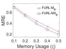
(a) Facebook

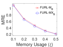
(b) Actor

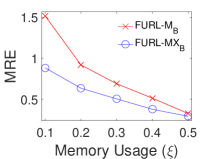
(c) Baidu

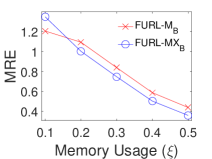
(d) DBLP-M

Figure 2: Mean of relative error vs. memory usage for Furl-MX${}_{\textsc{B}}$ and Furl-M${}_{\textsc{B}}$. Results with $\delta=$ 0.7, 0.4, 0.7, and 0.7 in Facebook, Actor, Baidu, and DBLP-M, respectively. Furl-MX${}_{\textsc{B}}$ gives the minimum error for a given memory usage in almost all cases.

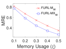
(a) Facebook

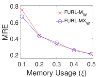
(b) Actor

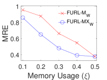
(c) Baidu

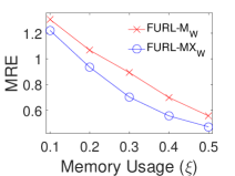
(d) DBLP-M

Figure 3: Mean of relative error vs. memory usage for Furl-MX${}_{\textsc{W}}$ and Furl-M${}_{\textsc{W}}$. Results with $\delta=$ 0.7, 0.1, 0.7, and 0.7 in Facebook, Actor, Baidu, and DBLP-M, respectively. Furl-MX${}_{\textsc{W}}$ gives the minimum error for a given memory usage in almost all cases.

Table 2: Datasets used in our experiments.

Name	Node	Edge	Description
Simple Graphs
YahooMsg2	100,000	587,963	User communication in Yahoo! messenger
Youtube1	1,138,499	2,990,287	Social network of Youtube users
Pokec1	1,632,803	22,301,964	Friendship network from Pokec
Skitter1	1,696,415	11,095,298	Autonomous system on the Internet
Hudong1	2,452,715	18,690,759	“related to” links in encyclopedia Hudong
WebGraph3	42,889,765	582,567,291	Hyperlinks in Web
Multigraphs
Facebook1	46,952	855,542	Wall posts on other user’s wall on Facebook
Actor1	382,219	33,115,812	Actor collaboration in movies
Baidu1	415,641	3,284,387	Baidu Encyclopedia ”related to” links
DBLP-M1	1,314,050	18,986,618	Co-author network in DBLP

¹http://konect.uni-koblenz.de/networks/
²http://webscope.sandbox.yahoo.com/catalog.php?datatype=g
³http://webdatacommons.org/hyperlinkgraph/#toc2

Evaluation Metric. The performances of algorithms are evaluated in the following two aspects.

Mean of Relative Error (MRE): This measures how an estimation is close to the ground truth.

$$\varepsilon(\tau,\varDelta)=\frac{1}{\left|V\right|}\sum_{u\in V}\frac{\left|\tau_{u}-\varDelta_{u}\right|}{{\varDelta_{u}+1}},$$

where $V$ is a set of nodes appearing in a graph stream. We add $1$ to the denominator for the case of $\varDelta_{u}=0$.

Proportion $\xi$ of Sampled Edges: This is the dominant factor of required memory spaces.

For all the algorithms, MRE is computed by the average of results obtained by $10$ independent runnings since they are randomized algorithms. The memory usage $\xi$ is determined as follows: for Furl-S, Furl-SX and Triest, $\xi=M/m$ where $m$ is the number of edges in a graph; for Mascot, $\xi=p$ where $p$ is a given edge sampling rate; for Furl-M and Furl-MX, $\xi=M/u$ where $u$ is the number of unique edges in a graph.

4.2 Accuracy for Simple Graph Stream

For simple graph stream, we compare Furl-S with two competing methods: Mascot LimK15 and Triest StefaniERU16 . Note that Triest is the same as Furl-S introduced in Section 3.1.

Figure 1 shows comparison between Furl-SX, Triest and Mascot in MRE over the memory usage $\xi$. We choose $\delta=0.7,0.1,0.4$, and $0.4$ in Youtube, Pokec, Skitter, and Hudong, respectively. As shown in the figure, Furl-SX gives the minimum error for a given memory usage compared to Triest and Mascot since Furl-SX gives more concentrated estimation around the ground truth.

4.3 Accuracy for Multigraph Stream

For multigraph stream, we compare only our proposed methods Furl-MX and Furl-M since there is no previous work.

Figure 2 shows the accuracy of Furl-MX${}_{\textsc{B}}$ and Furl-M${}_{\textsc{B}}$ for binary counting in MRE over the memory usage $\xi$. We present results with $\delta=0.7,0.4,0.7$, and $0.7$ for Facebook, Actor, Baidu, and DBLP-M, respectively. Note that Furl-MX${}_{\textsc{B}}$ gives the minimum error for a given memory usage in almost all cases since Furl-MX${}_{\textsc{B}}$ gives concentrated results.

Figure 3 shows comparison of Furl-MX${}_{\textsc{W}}$ and Furl-M${}_{\textsc{W}}$ for weighted counting in MRE over the memory usage $\xi$. We present results with $\delta=0.7,0.1,0.7$, and $0.7$ for Facebook, Actor, Baidu, and DBLP-M, respectively. As in the case of binary counting, Furl-MX${}_{\textsc{W}}$ outperforms Furl-M${}_{\textsc{W}}$, giving the minimum error for a given memory usage in almost all cases since Furl-MX${}_{\textsc{W}}$ gives concentrated results.

4.4 Anomaly Detection

In this section, we show anomalous patterns and nodes on real world graphs using Furl. The number of local triangles is an important index that indicates characteristics of nodes and cohesiveness of groups which neighbors of nodes form. We use two datasets YahooMsg and WebGraph listed in Table 2. YahooMsg is a user communication network in Yahoo! messenger whose edge means a user sends a message to another user. WebGraph is a hyperlink network of webpages. Its node and edge correspond to a web page and a hyperlink, respectively. Since they are simple graphs, we use Furl-SX with the following parameters: $\delta=0.4$, $\xi=0.01$ and $J=M$.

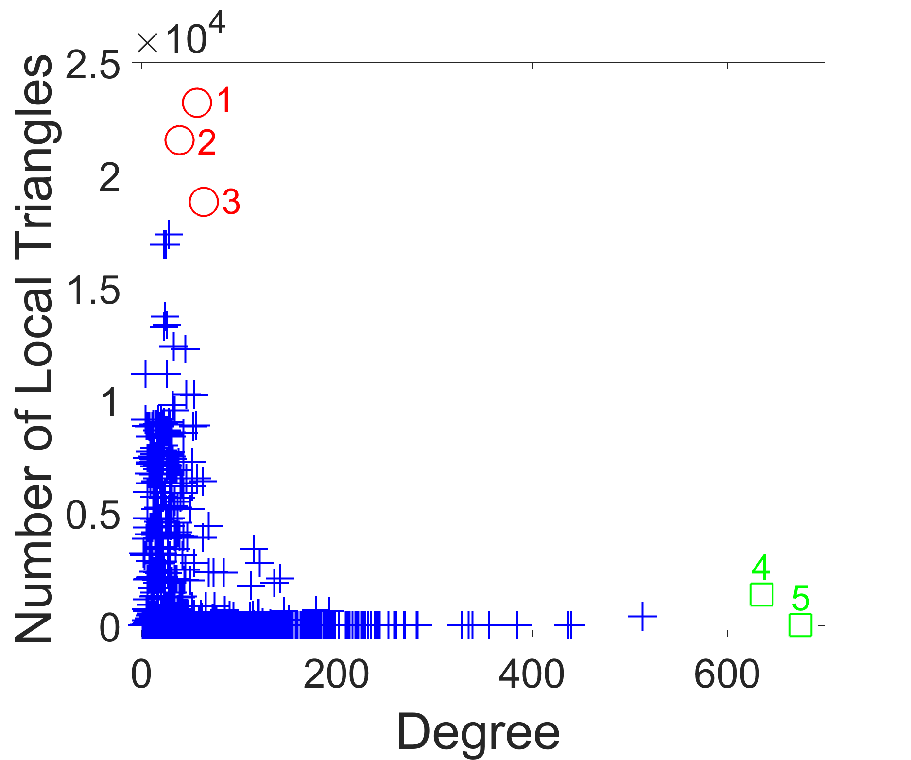
(a) YahooMsg

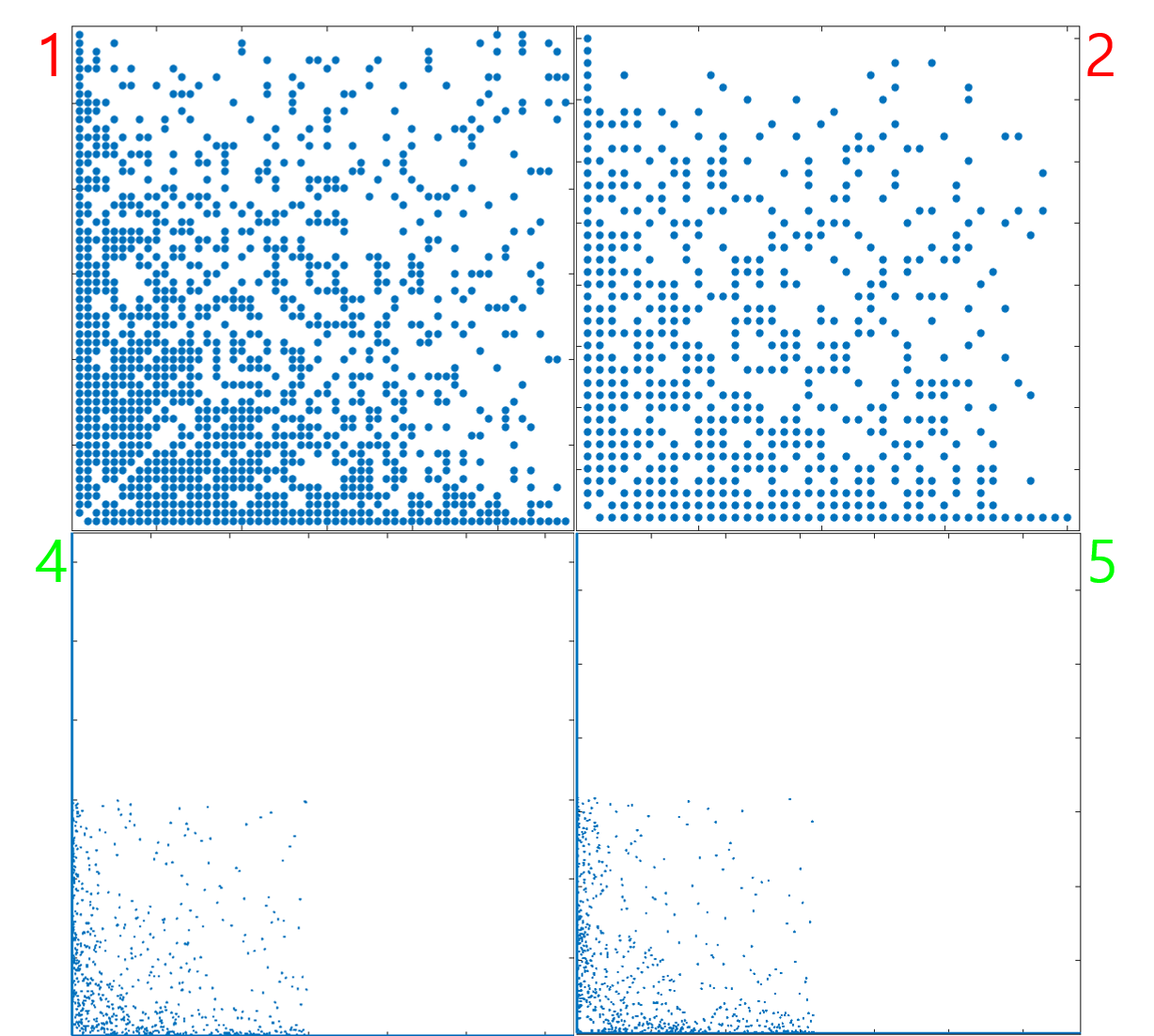
(b) Spyplots for egonets

Figure 4: (a) Degree vs. the number of local triangles estimated by Furl in YahooMsg. The neighbors of each red node contain a very large giant connected component; those of each green node have many tiny connected components. (b) Spyplots for the egonetworks of two red nodes (top) and two green nodes (bottom). Each spyplot at the top shows that the egonetworks are tightly connected. Each plot at the bottom represents that the egonetworks are loosely connected.

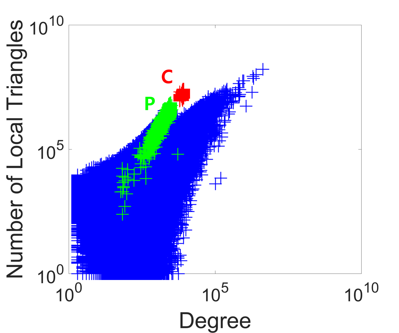
(a) WebGraph

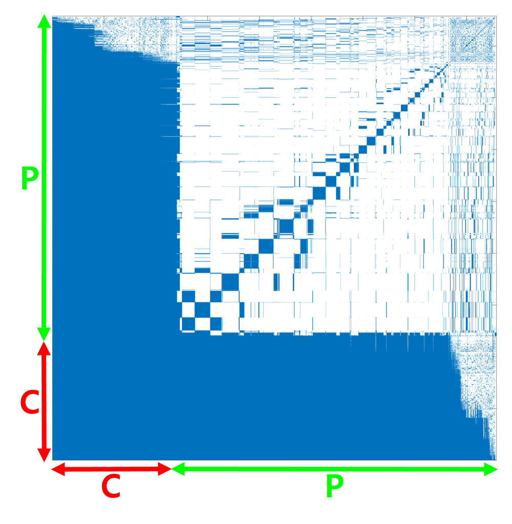
(b) Spyplot for C, P

Figure 5: (a) Degree vs. the number of local triangles estimated by Furl in WebGraph. The red group (marked ‘C’) forms a near-clique. The green group (marked ‘P’) corresponds to neighbors of the red nodes. Nodes in the green group have tight connections to the red group but are internally sparse. Both groups form a core-periphery structure. (b) Spyplot for the subgraph containing all red and green nodes. The core-periphery structure is clearly displayed.

Observation 1 (Single Large Neighbor Group)

In YahooMsg, there are users whose neighbors form a large connected group.

Observation 2 (Diverse Neighbor Groups)

In YahooMsg, there are users whose neighbors form diverse groups. The egonetwork of such user is a near-star network.

Figure 4a shows two anomalous patterns in YahooMsg. The first pattern, marked in red, corresponds to users whose neighbors form a large connected component. The second pattern, marked in green, corresponds to users whose neighbors form diverse groups. There are three users in the ”red” patterns and two users in the ”green” patterns (marked in Figure 4a). In the red patterns, neighbors of each of user1 and user2 make only one connected component, meaning that the users communicate within themselves. Two spyplots at the top of Figure 4b are those for the egonetworks of user1 and user2, respectively. The neighbors of user3 make two connected components, but about $94.6\%$ of the neighbors belong to one component. As a result, all users in the red pattern have tightly connected egonetworks.

In the green pattern, neighbors of the users make a number of groups. Two spyplots at the bottom of Figure 4b are spyplots for the egonetworks of user4 and user5, respectively. They demonstrate that the neighbors of each of user4 and user5 are hardly connected to each other. As a result, user4 has a near-star local structure. The neighbors of user4 form 357 connected components and their sizes are 1 or 2, except for 6 out of 357. The average size of the connected components is about 1.78. user5 shows a similar pattern. Its neighbors make 378 connected components and the average size of them is about 1.79.

Observation 3 (Core-periphery)

In WebGraph, there is a core-periphery structure which consists of two groups of nodes. One is a near-clique and the other is a sparse graph. The two subgraphs are tightly connected.

Figure 5a shows two groups “C” and “P” which are colored in red and green, respectively. Especially, the group C appears to be clearly separated from the rest of the graph in the figure. We find that the nodes in C are connected tightly. The number of the nodes in C is 2463 and their adjacency matrix has 2913 zeros. It means that there are only 225 missing edges: note that WebGraph has no self-loop. We also examine $6116$ neighbors of the nodes in C. Most of them are tightly connected with the nodes in C and we denote this neighbor group by “P”. The nodes in P are loosely connected with each other. To sum up, the nodes in C and P respectively form a near-clique and a sparse graph, and the nodes in P are tightly connected with the nodes in C, forming a core-periphery structure KangMF14 . Figure 5b is a spyplot of the nodes in C and P and shows they form a core-periphery.

5 Conclusion

In this paper, we propose Furl, an accurate algorithm for local triangle estimation in simple and multigraph streams. Furl handles graph streams of any sizes since it guarantees that the memory usage is fixed, and achieves high accuracy by reducing the variance of estimation. Our experimental results demonstrate that Furl-SX, the simple graph stream version of Furl, provides the best accuracy compared to the state-of-the-art algorithm. Furthermore, we show that Furl-MX, the multigraph stream version of Furl, performs well for graph streams with duplicate edges. Using Furl, we discover abnormal egonetworks like a near clique/star in a user communication network, and a core-periphery structure in the Web.

Appendix A Additional Analysis of FURL-SX

A.1 Lemma 4

Remind the following definitions:

$W(b_{\lambda})=(1-\delta)\delta^{B-b_{\lambda}}$.

$\phi(b_{\lambda})=\delta^{B-b_{\lambda}+1}$.

The equality examined here for $i\geq 1$ is as follows:

$$\mathbb{E}\left[Y_{\lambda}\right] =q_{\lambda}^{-1}\left(q_{\lambda}\sum_{b_{\lambda}\leq j\leq B}W(j)\right)$$

$$=\sum_{b_{\lambda}\leq j\leq B}W(j)$$

$$=(1-\delta)\delta^{B-b_{\lambda}}+(1-\delta)\delta^{B-b_{\lambda}-1}+\cdots+(1-\delta)$$

The last expression is the sum of the following geometric sequence from $n=1$ to $n=B-b_{\lambda}+1$:

$$a_{n}=(1-\delta)\delta^{n-1}.$$

The sum of the sequence is given by

$$\frac{(1-\delta)\left(1-\delta^{n}\right)}{1-\delta}.$$

Putting $n=B-b_{\lambda}+1$, by definition, we obtain

$$1-\delta^{B-b_{\lambda}+1}=1-\phi(b_{\lambda}).$$

A.2 Lemma 7

Let $\mu_{Y}$ and $\sigma_{Y}$ be the expectation and the variance of Furl-SX, respectively. Also, let $\mu_{X}$ and $\sigma_{X}$ be the expectation and the variance of Furl-S, respectively. We know the followings:

$$\mu_{Y} =\psi$$ (14)

$$\sigma_{Y}^{2} =\psi^{2}\left(q-1\right)$$ (15)

$$\mu_{X} =1$$ (16)

$$\sigma_{X}^{2} =\left(q-1\right),$$ (17)

where $\psi=1-\phi(b)$, and $\phi(b)=\delta^{B-i+1}$. Here, we omit the subscript to denote a certain triangle for simplicity. Using the Chebyshev inequality, we obtain

$$\Pr\left[|Y-\mu_{Y}|\geq\sigma_{Y}^{2}\right]\leq\frac{1}{\sigma_{Y}^{2}},$$ (18)

and thus,

$$\Pr\left[|Y-\mu_{X}|\geq\mu_{X}-\mu_{Y}+\sigma_{Y}^{2}\right] \leq\frac{1}{\sigma_{Y}^{2}}$$ (19)

$$\Pr\left[|Y-\mu_{X}|<\mu_{X}-\mu_{Y}+\sigma_{Y}^{2}\right] \geq 1-\frac{1}{\sigma_{Y}^{2}},$$ (20)

since $\mu_{Y}\leq\mu_{X}$. Similarly, we also derive the following inequality for $X$:

$$\Pr\left[|X-\mu_{X}|\geq\mu_{X}-\mu_{Y}+\sigma_{Y}^{2}\right] \leq\frac{\sigma_{X}^{2}}{(\mu_{X}-\mu_{Y}+\sigma_{Y}^{2})^{2}}$$ (21)

$$\Pr\left[|X-\mu_{X}|<\mu_{X}-\mu_{Y}+\sigma_{Y}^{2}\right] \geq 1-\frac{\sigma_{X}^{2}}{(\mu_{X}-\mu_{Y}+\sigma_{Y}^{2})^{2}}.$$ (22)

We want the following inequality holds:

$$1-\frac{1}{\sigma_{Y}^{2}} >1-\frac{\sigma_{X}^{2}}{(\mu_{X}-\mu_{Y}+\sigma_{Y}^{2})^{2}}$$ (23)

$$\frac{1}{\sigma_{Y}^{2}} <\frac{\sigma_{X}^{2}}{(\mu_{X}-\mu_{Y}+\sigma_{Y}^{2})^{2}}$$ (24)

$$1 <\frac{\sigma_{Y}^{2}\sigma_{X}^{2}}{(\mu_{X}-\mu_{Y}+\sigma_{Y}^{2})^{2}}$$ (25)

$$1 <\frac{\psi^{2}(q-1)^{2}}{(1-\psi+\psi^{2}(q-1))^{2}}$$ (26)

$$1 <\frac{\psi(q-1)}{1-\psi+\psi^{2}(q-1)}$$ (27)

$$1 >\frac{1-\psi+\psi^{2}(q-1)}{\psi(q-1)}$$ (28)

$$1 >\frac{1}{\psi(q-1)}-\frac{\psi}{\psi(q-1)}+\frac{\psi^{2}(q-1)}{\psi(q-1)}$$ (29)

$$1 >\frac{1}{\psi(q-1)}-\frac{1}{(q-1)}+\psi$$ (30)

$$1 >\frac{1}{q-1}\left(\frac{1}{\psi}-1\right)+\psi$$ (31)

$$1-\psi >\frac{1}{q-1}\left(\frac{1}{\psi}-1\right)$$ (32)

$$\phi >\frac{1}{q-1}\left(\frac{1-\psi}{\psi}\right)$$ (33)

$$\phi >\frac{1}{q-1}\left(\frac{\phi}{1-\phi}\right)$$ (34)

$$1-\phi >\frac{1}{q-1}$$ (35)

$$\frac{1}{1-\phi} <q-1$$ (36)

$$\frac{2-\phi}{1-\phi} <q$$ (37)

$$\frac{2-\delta^{B-b_{\lambda}+1}}{1-\delta^{B-b_{\lambda}+1}} <\frac{(T_{\lambda}-1)(T_{\lambda}-2)}{M(M-1)}$$ (38)

If we set $\delta=0.5$, this lemma states that every triangle appearing after $\approx 1.7M$ results in concentrated estimation.

References

- (1) Nesreen K. Ahmed, Nick G. Duffield, Jennifer Neville, and Ramana Rao Kompella. Graph sample and hold: a framework for big-graph analytics. In The 20th ACM SIGKDD International Conference on Knowledge Discovery and Data Mining, KDD ’14, New York, NY, USA - August 24 - 27, 2014, pages 1446–1455, 2014.
- (2) Noga Alon, Raphael Yuster, and Uri Zwick. Finding and counting given length cycles. Algorithmica, 17(3):209–223, 1997.
- (3) Shaikh Arifuzzaman, Maleq Khan, and Madhav V. Marathe. PATRIC: a parallel algorithm for counting triangles in massive networks. In 22nd ACM International Conference on Information and Knowledge Management, CIKM’13, San Francisco, CA, USA, October 27 - November 1, 2013, pages 529–538, 2013.
- (4) Ziv Bar-Yossef, Ravi Kumar, and D. Sivakumar. Reductions in streaming algorithms, with an application to counting triangles in graphs. In Proceedings of the Thirteenth Annual ACM-SIAM Symposium on Discrete Algorithms, January 6-8, 2002, San Francisco, CA, USA., pages 623–632, 2002.
- (5) Luca Becchetti, Paolo Boldi, Carlos Castillo, and Aristides Gionis. Efficient algorithms for large-scale local triangle counting. TKDD, 4(3), 2010.
- (6) Jonathan W Berry, Bruce Hendrickson, Randall A LaViolette, and Cynthia A Phillips. Tolerating the community detection resolution limit with edge weighting. Physical Review E, 83(5):056119, 2011.
- (7) Andrei Z. Broder, Moses Charikar, Alan M. Frieze, and Michael Mitzenmacher. Min-wise independent permutations (extended abstract). In Proceedings of the Thirtieth Annual ACM Symposium on the Theory of Computing, Dallas, Texas, USA, May 23-26, 1998, pages 327–336, 1998.
- (8) Luciana S. Buriol, Gereon Frahling, Stefano Leonardi, Alberto Marchetti-Spaccamela, and Christian Sohler. Counting triangles in data streams. In Proceedings of the Twenty-Fifth ACM SIGACT-SIGMOD-SIGART Symposium on Principles of Database Systems, June 26-28, 2006, Chicago, Illinois, USA, pages 253–262, 2006.
- (9) Bin-Hui Chou and Einoshin Suzuki. Discovering community-oriented roles of nodes in a social network. In Data Warehousing and Knowledge Discovery, 12th International Conference, DAWAK 2010, Bilbao, Spain, August/September 2010. Proceedings, pages 52–64, 2010.
- (10) Shumo Chu and James Cheng. Triangle listing in massive networks and its applications. In Proceedings of the 17th ACM SIGKDD International Conference on Knowledge Discovery and Data Mining, San Diego, CA, USA, August 21-24, 2011, pages 672–680, 2011.
- (11) Jonathan Cohen. Graph twiddling in a mapreduce world. Computing in Science and Engineering, 11(4):29–41, 2009.
- (12) Jean-Pierre Eckmann and Elisha Moses. Curvature of co-links uncovers hidden thematic layers in the world wide web. Proceedings of the national academy of sciences, 99(9):5825–5829, 2002.
- (13) Alessandro Epasto, Silvio Lattanzi, Vahab S. Mirrokni, Ismail Sebe, Ahmed Taei, and Sunita Verma. Ego-net community mining applied to friend suggestion. PVLDB, 9(4):324–335, 2015.
- (14) Xiaocheng Hu, Yufei Tao, and Chin-Wan Chung. Massive graph triangulation. In Proceedings of the ACM SIGMOD International Conference on Management of Data, SIGMOD 2013, New York, NY, USA, June 22-27, 2013, pages 325–336, 2013.
- (15) Madhav Jha, C. Seshadhri, and Ali Pinar. A space efficient streaming algorithm for triangle counting using the birthday paradox. In The 19th ACM SIGKDD International Conference on Knowledge Discovery and Data Mining, KDD 2013, Chicago, IL, USA, August 11-14, 2013, pages 589–597, 2013.
- (16) Hossein Jowhari and Mohammad Ghodsi. New streaming algorithms for counting triangles in graphs. In Computing and Combinatorics, 11th Annual International Conference, COCOON 2005, Kunming, China, August 16-29, 2005, Proceedings, pages 710–716, 2005.
- (17) Daniel M. Kane, Kurt Mehlhorn, Thomas Sauerwald, and He Sun. Counting arbitrary subgraphs in data streams. In Automata, Languages, and Programming - 39th International Colloquium, ICALP 2012, Warwick, UK, July 9-13, 2012, Proceedings, Part II, pages 598–609, 2012.
- (18) U. Kang, Brendan Meeder, Evangelos E. Papalexakis, and Christos Faloutsos. Heigen: Spectral analysis for billion-scale graphs. IEEE Trans. Knowl. Data Eng., 26(2):350–362, 2014.
- (19) Jinha Kim, Wook-Shin Han, Sangyeon Lee, Kyungyeol Park, and Hwanjo Yu. OPT: a new framework for overlapped and parallel triangulation in large-scale graphs. In International Conference on Management of Data, SIGMOD 2014, Snowbird, UT, USA, June 22-27, 2014, pages 637–648, 2014.
- (20) Konstantin Kutzkov and Rasmus Pagh. On the streaming complexity of computing local clustering coefficients. In Sixth ACM International Conference on Web Search and Data Mining, WSDM 2013, Rome, Italy, February 4-8, 2013, pages 677–686, 2013.
- (21) Matthieu Latapy. Main-memory triangle computations for very large (sparse (power-law)) graphs. Theor. Comput. Sci., 407(1-3):458–473, 2008.
- (22) Yongsub Lim and U. Kang. MASCOT: memory-efficient and accurate sampling for counting local triangles in graph streams. In Proceedings of the 21th ACM SIGKDD International Conference on Knowledge Discovery and Data Mining, Sydney, NSW, Australia, August 10-13, 2015, pages 685–694, 2015.
- (23) Ron Milo, Shai Shen-Orr, Shalev Itzkovitz, Nadav Kashtan, Dmitri Chklovskii, and Uri Alon. Network motifs: simple building blocks of complex networks. Science, 298(5594):824–827, 2002.
- (24) Rasmus Pagh and Francesco Silvestri. The input/output complexity of triangle enumeration. In Proceedings of the 33rd ACM SIGMOD-SIGACT-SIGART Symposium on Principles of Database Systems, PODS’14, Snowbird, UT, USA, June 22-27, 2014, pages 224–233, 2014.
- (25) Rasmus Pagh and Charalampos E. Tsourakakis. Colorful triangle counting and a mapreduce implementation. Inf. Process. Lett., 112(7):277–281, 2012.
- (26) Ha-Myung Park and Chin-Wan Chung. An efficient mapreduce algorithm for counting triangles in a very large graph. In 22nd ACM International Conference on Information and Knowledge Management, CIKM’13, San Francisco, CA, USA, October 27 - November 1, 2013, pages 539–548, 2013.
- (27) Ha-Myung Park, Francesco Silvestri, U. Kang, and Rasmus Pagh. Mapreduce triangle enumeration with guarantees. In Proceedings of the 23rd ACM International Conference on Conference on Information and Knowledge Management, CIKM 2014, Shanghai, China, November 3-7, 2014, pages 1739–1748, 2014.
- (28) A. Pavan, Kanat Tangwongsan, Srikanta Tirthapura, and Kun-Lung Wu. Counting and sampling triangles from a graph stream. PVLDB, 6(14):1870–1881, 2013.
- (29) Lorenzo De Stefani, Alessandro Epasto, Matteo Riondato, and Eli Upfal. Trièst: Counting local and global triangles in fully-dynamic streams with fixed memory size. In Proceedings of the 22nd ACM SIGKDD International Conference on Knowledge Discovery and Data Mining, San Francisco, CA, USA, August 13-17, 2016, pages 825–834, 2016.
- (30) AB Sunter. List sequential sampling with equal or unequal probabilities without replacement. Applied Statistics, pages 261–268, 1977.
- (31) Siddharth Suri and Sergei Vassilvitskii. Counting triangles and the curse of the last reducer. In Proceedings of the 20th International Conference on World Wide Web, WWW 2011, Hyderabad, India, March 28 - April 1, 2011, pages 607–614, 2011.
- (32) Siddharth Suri and Sergei Vassilvitskii. Counting triangles and the curse of the last reducer. In Proceedings of the 20th International Conference on World Wide Web, WWW 2011, Hyderabad, India, March 28 - April 1, 2011, pages 607–614, 2011.
- (33) Charalampos E. Tsourakakis, U. Kang, Gary L. Miller, and Christos Faloutsos. DOULION: counting triangles in massive graphs with a coin. In Proceedings of the 15th ACM SIGKDD International Conference on Knowledge Discovery and Data Mining, Paris, France, June 28 - July 1, 2009, pages 837–846, 2009.
- (34) Jeffrey Scott Vitter. Random sampling with a reservoir. ACM Trans. Math. Softw., 11(1):37–57, 1985.
- (35) Howard T. Welser, Eric Gleave, Danyel Fisher, and Marc A. Smith. Visualizing the signatures of social roles in online discussion groups. Journal of Social Structure, 8, 2007.
- (36) Zhi Yang, Christo Wilson, Xiao Wang, Tingting Gao, Ben Y. Zhao, and Yafei Dai. Uncovering social network sybils in the wild. In Proceedings of the 11th ACM SIGCOMM Internet Measurement Conference, IMC ’11, Berlin, Germany, November 2-, 2011, pages 259–268, 2011.