1 Experiments and Analysis
To supplement the illustrative synthetic examples, in this section we apply variational boosting to approximate various intractable posterior distributions resulting from real statistical analyses.
1.1 Hierarchical Binomial Regression
We test out our posterior approximation on a hierarchical binomial regression model.111Model and data from the mc-stan case studies, \urlhttp://mc-stan.org/documentation/case-studies/pool-binary-trials.html
We borrow an example from [efron1975data], and estimate the binomial rates of success (batting averages) of baseball players using a hierarchical model.
The model describes a latent “skill” parameter for baseball players — the probability of obtaining a hit in a given at bat.
The model of the data is
{align*}
ϕ&∼Unif \text hyper prior
κ∼Pareto(1, 1.5) \text hyper prior
θ_j ∼Beta(ϕ⋅κ, (1 - ϕ) ⋅κ) \text player prior
y_j ∼Binomial(K_j, θ_j) \text player hits
where is the number of successes (hits) player has attempted in attempts (at bats).
Each player has a latent success rate , which is governed by two global variables and .
There are 18 players in this example, creating a posterior distribution with parameters.
This model is not conjugate, and requires approximate Bayesian inference.
We use adam [kingma2014adam] for each stochastic optimization problem with default parameters. For stochastic gradients, we use 400 samples for the new component, and 400 samples for the previous component. In all experiments, we use autograd [autograd, maclaurin2015autograd] to obtain automatic gradients with respect to new component parameters.
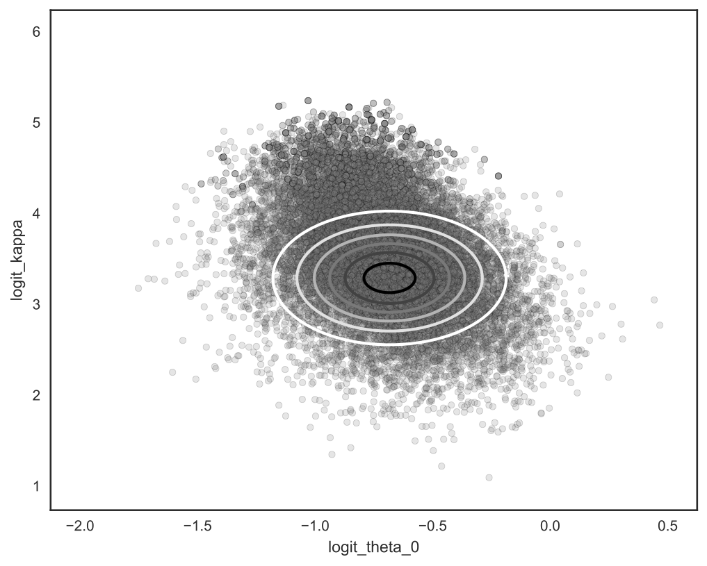
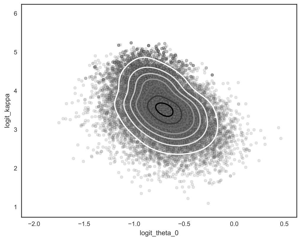
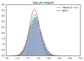
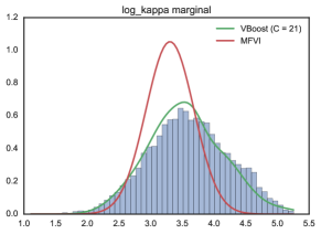
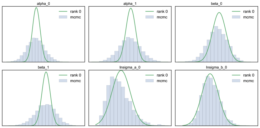
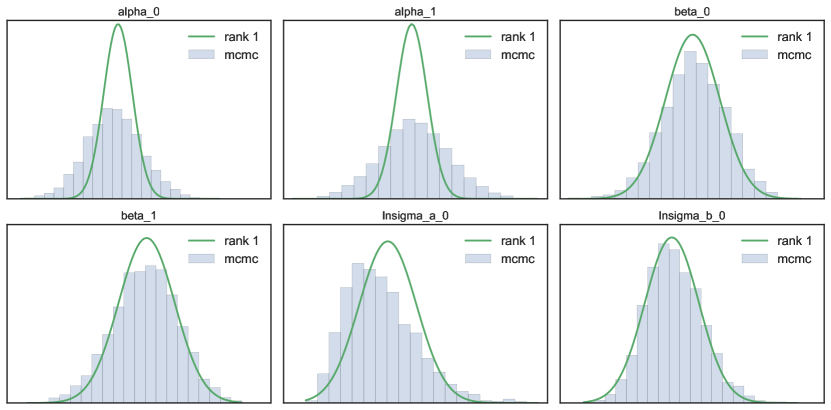
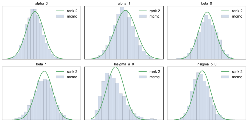
To highlight the fidelity of our method, we compare Variational Boosting to mean field VI and the No-U-Turn Sampler (NUTS) [hoffman2014no]. The empirical distribution resulting from 20k NUTS samples is considered the “ground truth” posterior in this example. Figure 1 compares a selection of univariate and bivariate posterior marginals. We see that Variational Boosting is able to closely match the NUTS posteriors, improving upon the MFVI approximation.
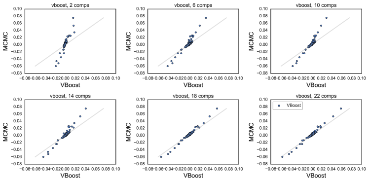
Figure 2 compares the variational boosting covariance estimates to the “ground truth” estimates of MCMC at various stages of the algorithm.
[b]0.45
 {subfigure}[b]0.45
[b]0.45
 {subfigure}[b]0.45
[b]

[b]1

[b]

[b]

1.2 Multi-level Poisson GLM
We apply variational boosting to approximate the posterior for a common hierarchical model, a hierarchical Poisson GLM. This model was formulated to measure the relative rates of stop-and-frisk events for different ethnicities and in different precincts [gelman2007analysis], and has been used as illustrative example of multi-level modeling [gelman2006data, Chapter 15, Section 1].
The model incorporates a precinct and ethnicity effect to describe the relative rate of stop-and-frisk events.
{align*}
μ&∼N(0, 10^2) \text mean offset
lnσ^2_α, lnσ^2_β ∼N(0, 10^2) \text group variances
α_e ∼N(0, σ^2_α) \text ethnicity effect
β_p ∼N(0, σ^2_β) \text precinct effect
lnλ_ep = μ+ α_e + β_p + lnN_ep \text log rate
Y_ep ∼P(λ_ep) \text stop-and-frisk events
where are the number of stop-and-frisk events within ethnicity group and precinct over some fixed period of time; is the total number of arrests of ethnicity group in precinct over the same period of time; and are the ethnicity and precinct effects.
[b]

[b]

[b].85
[b].85
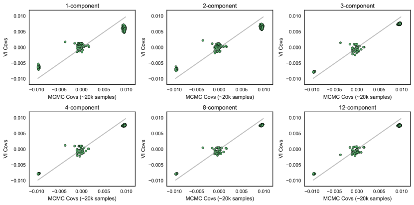
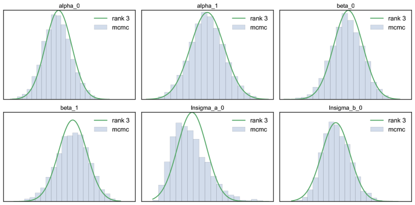
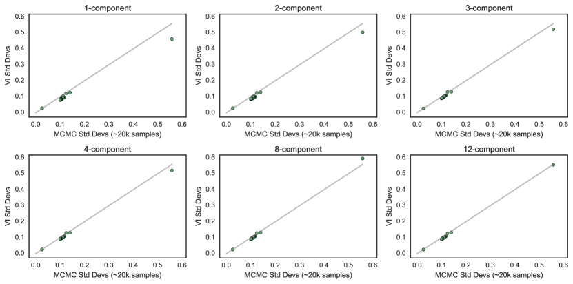
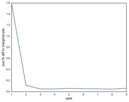
As before, we simulate 20k NUTS samples, and compare various variational approximations. Because of the high posterior correlations present in this example, variational boosting with diagonal covariance components is inefficient in its representation of this structure. As such, this example more heavily relies on the low-rank approximation to shape the posterior.
Figure 7 show how increasing the rank of a single multivariate normal component can result in better variance approximations. Figure 12 shows a handful of bivariate marginal posterior approximations as a function of covariance rank. Figure 15 shows the same bivariate marginals as more rank-3 components are added to the approximation. Lastly, Figure 18 compares the marginal standard deviations and covariances to MCMC-based measurements. These results indicate that while the incorporation of covariance structure increases the accuracy of marginal variance approximations, the non-Gaussianity afforded by the incorporation of mixture components allows for a better posterior approximation that translates into even more accurate moment estimates.
1.3 Bayesian Neural Network
Lastly, we apply our method to a Bayesian neural network regression model, which admits a high-dimensional, non-conjugate posterior. We compare predictive performance of Variational Boosting to Probabilistic Backpropagation (PBP) [hernandez2015probabilistic]. Mimicking the experimental setup of [hernandez2015probabilistic], we use a single 50-unit hidden layer, with ReLU activation functions. We place a normal prior over each weight in the neural network, governed by the same variance (with an inverse Gamma prior). We also place an inverse Gamma prior over the observation variance The model can be written as
| weight prior hyper | (1) | ||||
| noise prior hyper | (2) | ||||
| weights | (3) | ||||
| output distribution | (4) |
where is the set of weights, and is a multi-layer perceptron that maps input to approximate output as a function of parameters . We denote the set of parameters as . We approximate the posterior , where is the training set of input-output pairs. We then use the posterior predictive distribution to compute the distribution for a new input