Migration of Planets Into and Out of Mean Motion Resonances in Protoplanetary Disks: Analytical Theory of Second-Order Resonances

Abstract

Recent observations of Kepler multi-planet systems have revealed a number of systems with planets very close to second-order mean motion resonances (MMRs, with period ratio $1:3$, $3:5$, etc.) We present an analytic study of resonance capture and its stability for planets migrating in gaseous disks. Resonance capture requires slow convergent migration of the planets, with sufficiently large eccentricity damping timescale $T_{e}$ and small pre-resonance eccentricities. We quantify these requirements and find that they can be satisfied for super-Earths under protoplanetary disk conditions. For planets captured into resonance, an equilibrium state can be reached, in which eccentricity excitation due to resonant planet-planet interaction balances eccentricity damping due to planet-disk interaction. This “captured” equilibrium can be overstable, leading to partial or permanent escape of the planets from the resonance. In general, the stability of the captured state depends on the inner to outer planet mass ratio $q=m_{1}/m_{2}$ and the ratio of the eccentricity damping times. The overstability growth time is of order $T_{e}$, but can be much larger for systems close to the stability threshold. For low-mass planets undergoing type I (non-gap opening) migration, convergent migration requires $q\lesssim 1$, while the stability of the capture requires $q\gtrsim 1$. These results suggest that planet pairs stably captured into second-order MMRs have comparable masses. This is in contrast to first-order MMRs, where a larger parameter space exists for stable resonance capture. We confirm and extend our analytical results with $N$-body simulations, and show that for overstable capture, the escape time from the MMR can be comparable to the time the planets spend migrating between resonances.

1 Introduction

Planets formed in a gaseous protoplanetary disk excite density waves and experience back-reaction torques from the disk (Goldreich & Tremaine, 1979, 1980; Lin & Papaloizou, 1979). While the magnitude and sign of the torque depend on the planet’s mass, location and the physical property of the disk (e.g., Kley & Nelson 2012; Baruteau et al. 2014), some degrees of disk-driven migration are inevitable, especially for planets with gaseous atmosphere or envelope (including gas giants and “rocky” planets with radii $\gtrsim 2R_{\oplus}$) – the presence of the envelope indicates that these planets have formed before gas disks dissipate. Planets in multi-planet system generally have different migration rates, and their period ratio varies during migration. It has long been established that slow convergent migration can naturally result in neighboring planets captured into mean motion resonances (MMRs), in which the planet’s period ratio $P_{2}/P_{1}$ stays close to $j/(j-q)$ (where $q,j>q$ are positive integers) (e.g. Snellgrove et al. 2001; Lee & Peale 2002; see also Goldreich (1965) and Peale (1986) for studies of MMRs in the solar system). Therefore one would expect that an appreciable fraction of multi-planet systems reside in resonant configurations.

The Kepler mission has discovered thousands of super-Earths and sub-Neptunes (with radii 1.2-3$R_{\oplus}$) with periods less than 200 days, many of which are in multi-planet systems. The period ratios of a majority of these Kepler multi’s do not preferentially lie in or close to MMRs, although there is a significant excess of planet pairs with period ratios slightly larger (by about $1-2\%$) than that for exact resonance (Fabrycky et al., 2014). The discovery of several resonant chain systems (such as Kepler-223, with four planets in 3:4:6:8 MMRs; Mills et al. 2016) suggests that resonance capture during the “clean” disk-driven migration phase can be quite common, but subsequent physical processes may have destroyed the resonances for most systems. There have been many numerical studies on MMRs in protoplanetary disks, either using $N$-body integrations with fictitious forces that mimic dissipative effects (e.g., Lee & Peale 2002; Terquem & Papaloizou 2007; Rein & Papaloizou 2009; Rein 2012; Migaszewski 2015) or using self-consistent hydrodynamics (e.g. Kley et al. 2005; Papaloizou & Szuszkiewicz 2005; Crida et al. 2008; Zhang et al. 2014; André & Papaloizou 2016). A number of papers have studied possible mechanisms that could break migration-induced resonances, such as late dynamical instabilities following disk dispersal (e.g., Cossou et al. 2014; Pu & Wu 2015), planetesimal scattering (Chatterjee & Ford, 2015), and tidal dissipation in the planets (Papaloizou & Terquem, 2010; Lithwick & Wu, 2012; Batygin & Morbidelli, 2013; Lee et al., 2013). Regardless of whether MMRs are maintained or destroyed by any of these processes, it is important to recognize that MMRs play a significant role in the early evolution of planetary systems and can profoundly shape their final architectures. Therefore it is important to understand under what conditions resonance capture can occur or can be avoided when planets undergo disk-driven migration.

Recent theoretical works on resonance capture have focused on first-order ($j:j-1$) MMRs. While the basic dynamics of resonance capture was long understood (i.e., convergent migration with sufficiently slow rate leads to either secure or probabilistic resonance capture, depending on the initial, “pre-resonance” planet eccentricity; see, e.g., Henrard 1982; Borderies & Goldreich 1984; Lemaitre 1984a, b), a recent study by Goldreich & Schlichting (2014) revealed that, in the presence of the eccentricity damping due to planet-disk interaction, the long-term stability of MMRs can be compromised and resonance capture may be temporary. In particular, using a restricted three-body model (where the inner planet has a negligible mass), Goldreich & Schlichting (2014) showed that the equilibrium MMR state of the planets (in which eccentricity excitation due to resonant planet-planet interaction balances disk-induced eccentricity damping) can be overstable, and the system escapes the resonance on a timescale shorter than the migration timescale between resonances. A more complete analysis by Deck & Batygin (2015) (see also Batygin 2015) for planets with comparable masses suggested that a significant portion of the systems can be stably captured, and even for those exhibiting overstability, the timescale the planets spend in/near resonance could be comparable to the timescale the planets spend traveling between resonances.

While first-order MMRs for migrating planets have been studied in depth, second-order ($j:j-2$) MMRs pose an equally compelling problem. Among the observed multi-planet systems, there are a few pairs of planets that have period ratio very close to exact second-order resonances, including Kepler 365 ($P_{2}/P_{1}-5/3=8.7\times 10^{-4}$), Kepler 262 ($P_{2}/P_{1}-5/3=6.6\times 10^{-3}$), Kepler 87 ($P_{2}/P_{1}-5/3=4.3\times 10^{-5}$), Kepler 29 ($P_{2}/P_{1}-9/7=-4.4\times 10^{-5}$), and Kepler 417 ($P_{2}/P_{1}-9/7=7.2\times 10^{-3}$). It is unlikely that such a small deviation from commensurability is a result of random chance; rather, it suggests that these planet pairs are formed by resonance capture during migration. In addition, the population statistics of multi-planet systems has also revealed some signatures of second-order MMRs. While the period ratio distribution of Kepler multi’s exhibits the most prominent features near first-order MMRs (an excess at 3:2 and a deficit around 2:1; Fabrycky et al. 2014) and at the enigmatic ratio of 2.2 (Steffen & Hwang, 2015), the excess at the period ratio 1.7 ($\approx 5/3$) is also appreciable, and may be as significant as the 2:1 feature (see Fig. 20 of Steffen & Hwang 2015; J. Steffen, private communication). The period ratio distribution near second-order MMRs is also worth noting: Fig. 1 shows that there is a paucity of planets right inside the resonances [i.e. with period ratio close to, but smaller than, $j/(j-2)$]. Overall, these evidence suggests that second-order resonances are strong enough to influence the architecture of multi-planet systems, but they produce relatively few incidences of permanent capture.

Previous analytical studies on second and higher order MMRs are mostly in the context of solar system asteroids (e.g. Borderies & Goldreich 1984; Lemaitre 1984a, b). Recenty, Delisle et al. (2015) studied analytically the resonance capture problem for arbitrary order MMRs with planets pairs having finite masses. Using an approximated integrable Hamiltonian (Delisle et al., 2014), they derived a condition for stable capture in terms of the eccentricity damping timescales and equilibrium eccentricity ratio of the planets. They found that in order to make the captured MMR stable, the protoplanetray disk density profile often has to be locally inverted (i.e. the surface density increases outwards). Other studies of second-order MMRs for planets migrating in protoplanetary disks (e.g. Nelson & Papaloizou 2002; Xiang-Gruess & Papaloizou 2015) have largely relied on numerical experiments. While valuable, these numerical experiments are typically tailored toward particular systems or setups, and it is often difficult to know how the results depend on the physical inputs or parameters. There is also a common preconception that capture into second-order MMRs is difficult because the planet perturbation associated with a second-order resonance is too weak to counter the eccentricity damping from planet interaction with the disk.

In this paper and the companion paper, we develop an analytic theory to study the capture and stability/escape of second-order MMRs for planets pairs migrating in protoplanetary disks. Unlike the first-order MMR, the Hamiltonian for the second-order MMR (for comparable mass planet pairs) is generally non-integrable. We treat this Hamiltonian exactly using a semi-analytic approach. We also compare our analytic results to numerical $N$-body experiments. Our goal is to derive the conditions for resonance capture and the long-term stability of the resonance, to understand the similarities and differences between first and second-order MMRs, and to shed light on the observed properties of MMRs in multi-planet systems.

Our paper is organized as follows. In Sections 2 and 3, we consider second-order MMRs in the restricted three-body problem, where the inner or outer planet is massless. For such restricted problems, the resonant Hamiltonian can be reduced to that of a one degree of freedom system. We use the reduced Hamiltonian to review the resonance capture mechanism and the stability of the equilibrium state. In Section 4, we discuss the resonance capture criteria (in terms of planet masses, migration and eccentricity damping rates), and we examine whether planet migration in disks could allow resonance capture and explain the observed Kepler super-Earths in second-order MMRs. In Section 5, we advance to the general case when the two planets have comparable masses, analyzing the capture mechanism and finding the criterion for stable capture. The stable capture criterion is compared to the result of Delisle et al. (2015). Since the second-order resonance Hamiltonian in this general case cannot be reduced to that of a one degree of freedom system, the analysis of resonance capture and stability is considerably more complicated than the restricted problems, and we relegate much of the technical details to Appendix A (available online). In Section 6, we perform N-body simulations of migrating planets and compare with our analytic results derived in Sections 2-5. In Section 7 we summarize our key results and discuss their implications.

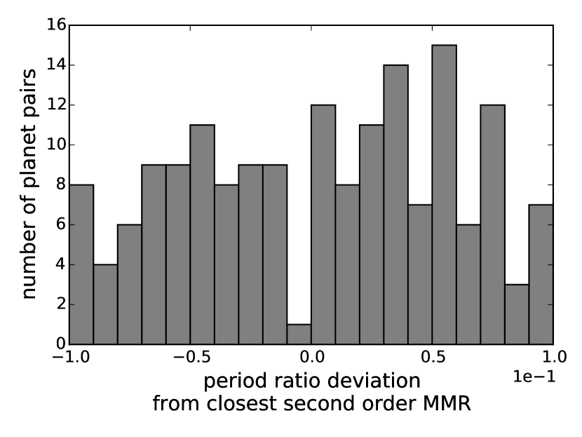
Figure 1: Distribution of the period ratio deviation from the closest second-order MMR ($j:j-2$) with $j\leq 9$ for the observed multi-planet systems. Data from exoplanet.org is used. The deviation is given by $P_{2}/P_{1}-j/(j-2)$, where $P_{i}$ are the periods of the planets. We see a paucity of planets just inside the resonance: For period ratio deviation in the range of $[-0.01,0]$, there is only one pair of planets, and this value is $3\sigma$ below the average.

2 Resonance in Restricted Three-Body Problem: Small Inner Planet

Consider a system with two planets with mass $m_{1},m_{2}$ orbiting around a star with mass $M_{\star}$. Assume $a_{1}<a_{2}$, and let $\alpha\equiv a_{1}/a_{2}<1$ be the semi-major axis ratio. In this section we will consider the case when the inner planet’s mass is negligible ($m_{1}\ll m_{2}$). We assume $e_{2}=0$ and $e_{1}$ is small. Most of the results in this section has been covered in previous studies (e.g. Delisle et al. 2014, 2015). Here we review this problem to prepare for the following discussion on capture criteria (Section 4) and the general problem with comparable mass planets (Section 5).

2.1 Hamiltonian

At small eccentricity, the system’s Hamiltonian $H$ near a $j:j-2$ MMR can be reduced to the following dimensionless form

$$\begin{split}-H=\eta\Theta+\Theta^{2}+\Theta\cos\theta,\end{split}$$ (1)

where $\theta$ and $\Theta$ are a pair of conjugate coordinate and momentum, and $\eta$ is the “resonance” parameter. They are given by

$$\theta=j\lambda_{2}+(2-j)\lambda_{1}-2\varpi_{1},$$ (2)

$$\Theta=\frac{3(j-2)^{2}}{16f_{d}\mu_{2}\alpha_{0}}\left(1-\sqrt{1-e_{1}^{2}}\right)\sim\mu_{2}^{-1}e_{1}^{2},$$ (3)

$$\eta\simeq\frac{1}{4f_{d}\mu_{2}}\left[(j-2)\alpha_{0}^{-1}-j\alpha_{0}^{1/2}\right],$$ (4)

where $\mu_{2}=m_{2}/M_{\star}$. The parameter $\alpha_{0}$ is related to $\alpha=a_{1}/a_{2}$ by

$$\begin{split}\alpha_{0}\equiv\alpha[1+(j-2)e_{1}^{2}/2],\end{split}$$ (5)

and is conserved because it is a function of a fast angle’s conjugate momentum. Here $f_{d}$ is a function of $\alpha$ evaluated at $\alpha_{0}$, and is of order unity. Murray & Dermott (1999) gives the expression of $f_{d}$ in Table 8.1, and the derivation of the above Hamiltonian and conserved quantities can also be found in that book. In the dimensionless Hamiltonian, time is scaled to

$$\begin{split}\tau=4f_{d}\alpha_{0}\mu_{2}n_{1}t\equiv t/T_{0},\end{split}$$ (6)

with

$$\begin{split}T_{0}=(4f_{d}\alpha_{0}\mu_{2}n_{1})^{-1}.\end{split}$$ (7)

The phase space topology of the Hamiltonian (1) gives useful information about the structure of the resonance. Figure 2 shows the level curves of the Hamiltonian for different $\eta$ values, plotted in the phase space of the conjugate variables $X=\sqrt{2\Theta}\cos\theta$ and $Y=\sqrt{2\Theta}\sin\theta$. Note that the distance to the origin is $\sqrt{X^{2}+Y^{2}}=\sqrt{2\Theta}$, which is proportional to $e_{1}$. There can be at most three fixed points, located at $Y=0$ and $X=0$, $X=-\sqrt{1-\eta}$ (for $\eta<1$) and $X=\sqrt{-1-\eta}$ (for $\eta<-1$), and their distances to the origin as a function of $\eta$ are shown in Figure 3. Two bifurcations take place as $\eta$ increases from $\eta\ll-1$: at $\eta=-1$ the unstable fixed point ($X=\sqrt{-1-\eta}$) merges with the origin, making the origin unstable; at $\eta=1$ the stable fixed point ($X=-\sqrt{1-\eta}$) merges with the origin (which is now unstable), making the origin stable again. For $\eta<-1$ or $\eta>1$, the origin is a stable fixed point and orbit with low eccentricity stays at low eccentricity. For $-1<\eta<1$, on the other hand, planets with initially near circular orbit will exhibit oscillating eccentricity, with a maximum $\Theta\sim 1-\eta$ [corresponding to $e_{1}\sim\mu_{2}^{1/2}(1-\eta)^{1/2}]$. The width of the resonance can be defined as the range of $\alpha_{0}$ for which $-1<\eta<1$; since $|\partial\eta/\partial\alpha_{0}|\sim\mu_{2}^{-1}$, the width in terms of $\alpha_{0}$ is $\sim\mu_{2}$. This width of resonance is small, which means that few planets would be in resonance if they are formed completely in situ.

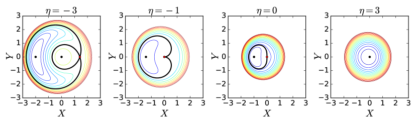
Figure 2: Level curves of the Hamiltonian (1) for different $\eta$, plotted in the phase space of the conjugate variables $X=\sqrt{2\Theta}\cos\theta$ and $Y=\sqrt{2\Theta}\sin\theta$ (see Section 2.1). The thick black line in each panel marks the separatrix; the black (red) dots mark the stable (unstable) fixed points.

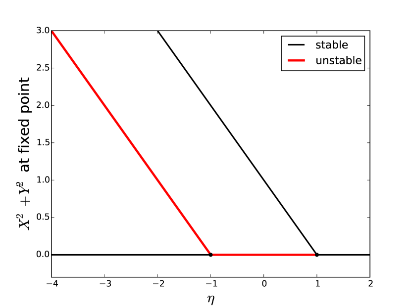
Figure 3: Locations of the fixed points as a function of $\eta$ (see Section 2.1). The vertical axis shows the (squared) distance between the fixed point and the origin, $X^{2}+Y^{2}=2\Theta$, which is proportional to $e_{1}^{2}$. Bifurcations occur at $\eta=1$ and $\eta=-1$. The stability of the fixed points are marked by color; the red intervals are unstable.

2.2 Eccentricity excitation and resonance capture

The Hamiltonian (1) only includes the non-dissipative resonant interaction between the two planets. In real systems, the planets can experience (dissipative) perturbations from other sources, e.g. planet-disk interaction. When the resonant interaction between the planets is dominant (i.e. the characteristic timescales of other perturbations are all $\gg T_{0}$), the effects of the other perturbations can be included as a slow variation of $\eta$, with $|d\eta/d\tau|\ll 1$. Therefore, it is helpful to first study how the system evolves when it passes the resonance as $\eta$ slowly increases/decreases [see, e.g. Borderies & Goldreich (1984); Xu & Lai (2016)]. We assume that the initial (out-of-resonance) eccentricity of the planet (test mass) is sufficiently small such that $\Theta_{0}\ll 1$, or equivalently $e_{0}\ll\mu_{2}^{1/2}$. The two possibilities are

(i) When the system passes resonance from $\eta<-1$ (i.e. $\eta$ is slowly increasing), the planet’s eccentricity is excited at $\eta=-1$ because the origin ($\Theta=0$) becomes unstable. After that, the phase space area bounded by the trajectory is conserved because the evolution is adiabatic. This area is of order unity, therefore the system ends up with a final eccentricity $\Theta_{f}\sim 1$ or $e_{f}\sim\sqrt{\mu_{2}}$. Note that the system is not in resonance, since the resonant angle $\theta$ is circulating.

(ii) On the other hand, when the system passes resonance from $\eta>1$ (i.e. $\eta$ slowly decreasing), the planet can be captured into resonance. This is because as $\eta$ goes below $1$, the origin becomes unstable and the stable fixed point moves away from the origin. When $|d\eta/d\tau|\ll 1$, the system follows this stable fixed point (with $2\Theta=1-\eta$) and advects into the libration zone with a finite eccentricity. The eccentricity excited by this resonant advection is unbounded as long as $\eta$ keeps decreasing and the small eccentricity approximation holds.

2.3 Effect of planet migration

We now analyze the effect of planet migration due to interaction with a protoplanetary disk. The dissipative effect of planet-disk interaction can be parameterized by

$$\left.\frac{1}{a_{i}}\frac{da_{i}}{dt}\right|_{\rm diss}=-\frac{1}{T_{m,i}}-\frac{p_{i}e_{i}^{2}}{T_{e,i}},$$ (8)

$$\left.\frac{1}{e_{i}}\frac{de_{i}}{dt}\right|_{\rm diss}=-\frac{1}{T_{e,i}},$$ (9)

where $T_{m,i}$ and $T_{e,i}$ (with $i=1,2$) characterize the timescale of inward migration and eccentricity damping; and we define the dimensionless timescales $\tau_{m,i}\equiv T_{e,i}/T_{0},\tau_{e,i}\equiv T_{e,i}/T_{0}$. For small (non-gap-opening) planets in a gaseous disk, these timescales are given by (e.g. Ward 1997; Goldreich & Schlichting 2014)

$$T_{m,i}^{-1}\sim\mu_{i}\mu_{d,i}\left(\frac{a_{i}}{h_{i}}\right)^{2}n_{i},$$ (10)

$$T_{e,i}^{-1}\sim\mu_{i}\mu_{d,i}\left(\frac{a_{i}}{h_{i}}\right)^{4}n_{i},$$ (11)

where $\mu_{d,i}=\Sigma_{d}a_{i}^{2}/M_{\star}$ is disk to star mass ratio and $h_{i}$ is the disk’s scale hight at $a_{i}$. For an Earth-mass planet at $a_{i}\sim 0.5$AU, with $\mu_{d,i}\sim 10^{-4}$ and $h_{i}/a_{i}\sim 0.1$, the migration time $T_{m.i}$ is of order 1Myr, while $T_{e,i}\sim 10^{4}$yrs. The actual value of $T_{m,i}$ and $T_{e,i}$ are uncertain since they depend on the thermodynamic property and profile of the disk (e.g. Baruteau et al. 2014). The parameter $p_{i}$ characterizes the energy dissipation rate associated with eccentricity damping, and usually $p_{i}\simeq 2$.

Noting that $\partial\eta/\partial\alpha_{0}<0$, $d\ln\alpha_{0}/d\tau=d\ln\alpha/d\tau+(j-2)e_{1}(de_{1}/d\tau)$, and using Eqs. (8) - (9) we find

$$\begin{split}\frac{d\eta}{d\tau}=\left|\frac{\partial\eta}{\partial\ln\alpha_{0}}\right|\left[-\frac{1}{\tau_{m}}+\frac{(p_{1}+j-2)e_{1}^{2}}{\tau_{e}}\right],\end{split}$$ (12)

where $\tau_{e}\equiv\tau_{e,1}$ and

$$\begin{split}\frac{1}{\tau_{m}}\equiv-\frac{1}{\tau_{m,1}}+\frac{1}{\tau_{m,2}}.\end{split}$$ (13)

Note that $\tau_{e},\tau_{m}$ correspond to the physical timescales $T_{e}=T_{0}\tau_{e}$ and $T_{m}=T_{0}\tau_{m}$. To capture the system in resonance, we require $T_{m}>0$, i.e. $T_{m,1}>T_{m,2}$. We will focus on this (convergent migration) case in the remainder of this paper.

From Eq. (12) we see that when the eccentricity grows to a certain value, the second term in $d\eta/d\tau$ balances the first term and the system enters an equilibrium state. Therefore, the eccentricity will not grow unbounded and the system can be trapped in the resonance with a fixed $\eta$ (corresponding to a fixed period ratio) for a long time. In this equilibrium state,

$$\begin{split}e_{1,\rm eq}=\sqrt{\frac{\tau_{e}}{(p_{1}+j-2)\tau_{m}}}.\end{split}$$ (14)

2.4 Stability of capture

Planet migration and eccentricity damping due to planet-disk interaction are responsible for resonance capture and the establishment of the equilibrium; they also affect the stability of the equilibrium.

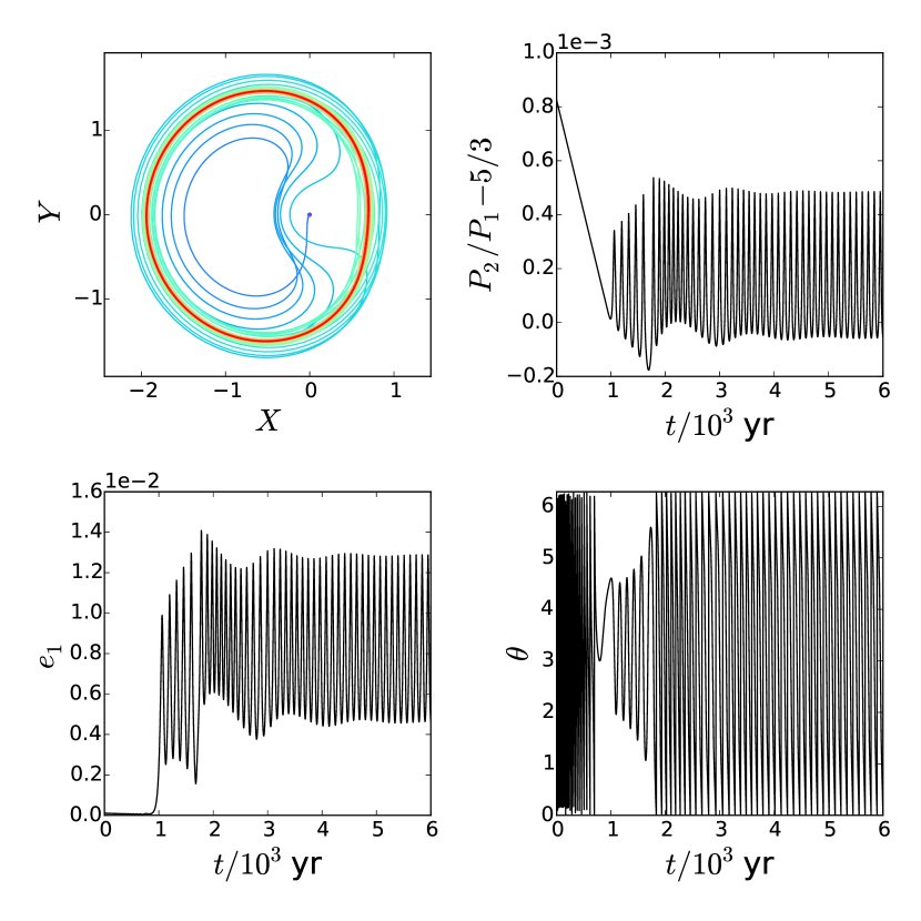
Figure 4: Evolution of a system near 3:5 mean motion resonance with $M_{\star}=1M_{\odot},m_{2}=10M_{\oplus},m_{1}\ll m_{2}$, and $a_{1}=0.1$AU (see Section 2.4). The migration and eccentricity damping timescales are $T_{m}=3$Myr and $T_{e}=1$kyr, corresponding to $\eta_{\rm eq}=-0.52$. The upper left panel shows the phase space trajectory, with time marked by color (blue indicates earlier time, followed by green, and red indicates later time); the upper right panel shows the deviation of period ratio $P_{2}/P_{1}$ from the exact resonance; the lower panels show the evolution of eccentricity and resonant angle $\theta$. We see that as the system is captured into resonance (with $\theta$ librating) at $t\sim 1$kyr. However, the phase space area bounded by the trajectory and the libration amplitude of $\theta$ increase due to overstability. This eventually pushes the system out of resonance ($\theta$ begins circulating at $t\simeq 2$kyr). The system ends up in an quasi-equilibrium state with the period ratio and eccentricity oscillating at fixed amplitudes.

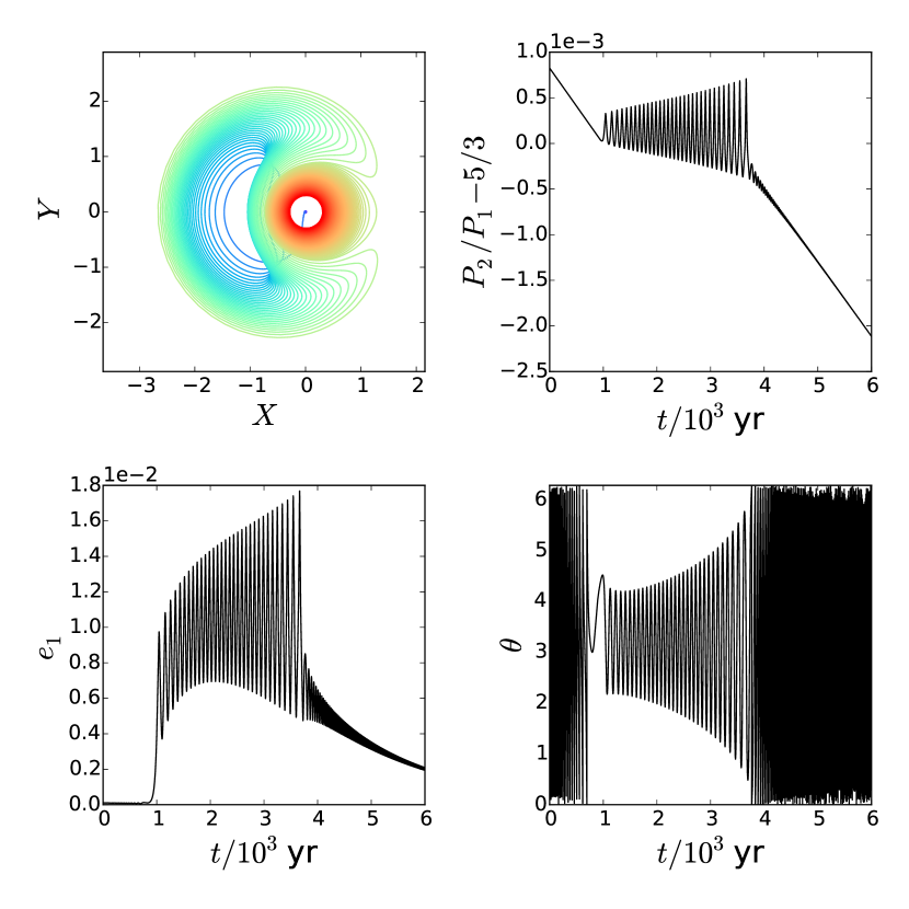
Figure 5: Same as Figure 2, except that $T_{e}$ is increased to 2kyr, giving $\eta_{\rm eq}=-1.27$ (see Section 2.4). In this case, the system enters the inner circulating zone upon exiting the libration zone. Eventually, the period ratio is no longer held near the equilibrium, and the eccentricity excited in resonance is quickly damped due to planet-disk interaction.

The equations of motion of the system near the MMR is determined by the Hamiltonian (1). Including the eccentricity damping term due to planet-disk interaction, we have

$$\dot{\Theta}=-\Theta\sin\theta-\frac{2}{\tau_{e}}\Theta,$$ (15)

$$\dot{\theta}=-\eta-2\Theta-\cos\theta,$$ (16)

where $\dot{\Theta}=d\Theta/d\tau$ and $\dot{\theta}=d\theta/d\tau$. In addition, the parameter $\eta$ evolves according to Eq. (12), or

$$\begin{split}\dot{\eta}=-\frac{\beta}{\tau_{m}}+\frac{4(p_{1}+j-2)}{(j-2)\tau_{e}}\Theta,\end{split}$$ (17)

where

$$\begin{split}\beta\equiv\left|\frac{\partial\eta}{\partial\ln\alpha_{0}}\right|\simeq\frac{3}{8f_{d}\mu_{2}}j^{2/3}(j-2)^{1/3}.\end{split}$$ (18)

Note that $\Theta=[(j-2)\beta/4]e^{2}$. For slow migration, $\beta/\tau_{m}$ and $1/\tau_{e}$ are both very small. The equilibrium point, to lowest order, is given by

$$\Theta_{\rm eq}=\frac{(j-2)\beta\tau_{e}}{4(p_{1}+j-2)\tau_{m}},$$ (19)

$$\theta_{\rm eq}\simeq\pi+\frac{2}{\tau_{e}},$$ (20)

$$\eta_{\rm eq}\simeq 1-2\Theta_{\rm eq}.$$ (21)

The linearized equations are (with $\Theta=\Theta_{\rm eq}+\delta\Theta$ and so on)

$$\begin{split}&\delta\dot{\Theta}=\Theta_{\rm eq}\delta\theta,\\ &\delta\dot{\theta}=-\delta\eta-2\delta\Theta-\frac{2}{\tau_{e}}\delta\theta,\\ &\delta\dot{\eta}=\frac{4(p_{1}+j-2)}{(j-2)\tau_{e}}\delta\Theta,\end{split}$$ (22)

and the characteristic equation is (for $\delta\Theta,\delta\theta,\delta\eta\propto e^{\lambda t}$)

$$\begin{split}\lambda^{3}+\frac{2}{\tau_{e}}\lambda^{2}+2\Theta_{\rm eq}\lambda+\frac{\beta}{\tau_{m}}=0.\end{split}$$ (23)

It is easy to see that the system has one negative real eigenvalue and two complex eigenvalues. We can assume $\Theta_{\rm eq}\gtrsim 1$ (corresponding to $\eta_{\rm eq}\lesssim-1$; otherwise the system can always stay captured; see below and Figure 2), and we notice $\tau_{e}^{-1},\beta/\tau_{m}\sim\Theta_{\rm eq}/\tau_{e}\ll 1$; therefore the complex eigenvalues are approximately

$$\begin{split}\lambda\simeq\lambda_{r}\pm i\sqrt{2\Theta_{\rm eq}},\end{split}$$ (24)

where the real part $\lambda_{r}$ is small ($|\lambda_{r}|\sim\tau_{e}^{-1}$). Substituting this back to (23) gives

$$\begin{split}\lambda_{r}\simeq\frac{p_{1}}{(j-2)\tau_{e}}.\end{split}$$ (25)

This indicates that the oscillation around the equilibrium is overstable for all realistic ($p_{1}>0$) situations. This agrees with the result of Delisle et al. (2015).

When the oscillation near the equilibrium is overstable, the phase space area bounded by the trajectory will eventually exceed the area of the libration zone and the system will be pushed out of resonance. Whether the system can maintain an approximately constant period ratio depends on the value of $\eta$ at the equilibrium state.

Figure 2 shows an example when $\eta_{\rm eq}>-1$. In this case, after resonance capture, the system is pushed into the outer circulation zone due to overstability. However, $\eta$ is still held near the equilibrium value because the eccentricity excitation forced by the unstable origin can balance the eccentricity damping. Therefore, $\alpha$ (and the period ratio) is still held approximately constant despite the fact that the system, strictly speaking, is not in resonance. Note that the condition $\eta_{\rm eq}>-1$ requires

$$\begin{split}\Theta_{\rm eq}=\frac{3}{32}\frac{j^{2/3}(j-2)^{4/3}}{(p_{1}+j-2)f_{d}}\mu_{2}^{-1}\frac{T_{e}}{T_{m}}<1,\end{split}$$ (26)

which corresponds to

$$\begin{split}\frac{T_{e}}{T_{m}}\lesssim\mu_{2}\end{split}$$ (27)

Since $T_{e}/T_{m}\sim(h/a)^{2}\sim 10^{-3}$ - $10^{-2}$, this condition can be satisfied only for massive planets ($\mu_{2}\gtrsim 10^{-3}$ - $10^{-2}$).

When $\eta_{\rm eq}<-1$, however, the system will eventually enter the circulation zone centered at the origin, as is shown in Figure 5. Within this zone, there is no eccentricity excitation mechanism and the eccentricity decreases. As a result, the system’s eccentricity can no longer hold $\eta$ near the equilibrium, and the period ratio increasingly deviates from the resonant value. In this case, the system stays near resonance for a duration of order

$$\begin{split}T_{0}|\lambda_{r}|^{-1}\sim T_{0}\tau_{e}=T_{e}.\end{split}$$ (28)

Since we know that $T_{e}\ll T_{m}$, while $T_{m}$ is the timescale for migrating between resonances, the system should be out of resonance for most of the time.

3 Resonance in Restricted Three-Body Problem: Small Outer Planet

Next we consider the case when the inner planet is more massive and the outer planet has negligible mass, i.e. $m_{1}\gg m_{2}$. This case can be illuminating since previous studies (Delisle et al., 2015; Deck & Batygin, 2015) already showed that the behavior of the system, especially the stability of capture, may depend on the mass ratio.

Similar to Section 2, the Hamiltonian can be written in the form of Eq. (1), but with the time scaled to

$$\begin{split}\tau=4f_{d}\mu_{1}n_{2}t\equiv t/T_{0},\end{split}$$ (29)

where $\mu_{1}=m_{1}/M_{\star}$. The conjugate variables and the “resonance” parameter are

$$\theta=j\lambda_{2}+(2-j)\lambda_{1}-2\varpi_{2},$$ (30)

$$\Theta=\frac{3j^{2}}{16f_{d}\mu_{1}}\left(1-\sqrt{1-e_{2}^{2}}\right),$$ (31)

$$\eta\simeq\frac{1}{4f_{d}\mu_{1}}\left[(j-2)\alpha_{0}^{-3/2}-j\right],$$ (32)

where $\mu_{1}=m_{1}/M_{\star}$, and

$$\begin{split}\alpha_{0}\equiv\alpha(1+je_{2}^{2}/2)\end{split}$$ (33)

is conserved.

With $\partial\eta/\partial\alpha_{0}<0$, we have

$$\begin{split}\frac{d\eta}{d\tau}=\left|\frac{\partial\eta}{\partial\ln\alpha_{0}}\right|\left[-\frac{1}{\tau_{m}}+\frac{(j-p_{2})e_{2}^{2}}{\tau_{e}}\right],\end{split}$$ (34)

where $\tau_{m}$ is the same as in Eq. (13) while $\tau_{e}\equiv\tau_{e,2}$. Resonance capture still occurs when the outer planet migrates inward more quickly (i.e. convergent migration), and the equilibrium eccentricity is

$$\begin{split}e_{2,\rm eq}=\sqrt{\frac{\tau_{e}}{(j-p_{2})\tau_{m}}}.\end{split}$$ (35)

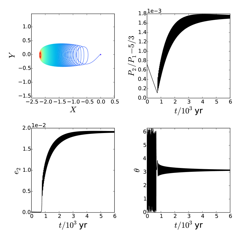
Figure 6: Evolution of a system near 3:5 mean motion resonance with $M_{\star}=1M_{\odot},m_{1}=10M_{\oplus},m_{2}\ll m_{1}$, and $a_{1}=0.1$AU (see Section 3.3). The migration and eccentricity damping timescales are $T_{m}=3$Myr and $T_{e}=1$kyr. We see that the system quickly approaches the equilibrium state, and the libration amplitude of $\theta,e$ and period ratio decrease. In the end, the system’s trajectory converges to the fixed point, and $\theta=\pi$.

The equations of motion are still given by Eqs. (15) - (16), while (17) is replaced by

$$\begin{split}\dot{\eta}=-\frac{\beta}{\tau_{m}}+\frac{4(j-p_{2})}{j\tau_{e}}\Theta,\end{split}$$ (36)

where

$$\begin{split}\beta\equiv\left|\frac{\partial\eta}{\partial\ln\alpha_{0}}\right|\simeq\frac{3j}{8f_{d}\mu_{1}}.\end{split}$$ (37)

The equilibrium eccentricity is given by

$$\Theta_{\rm eq}=\frac{j\beta\tau_{e}}{4(j-p_{2})\tau_{m}},$$ (38)

and the characteristic equation is

$$\begin{split}\lambda^{3}+\frac{2}{\tau_{e}}\lambda^{2}+\frac{j\beta\tau_{e}}{2(j-p_{2})\tau_{m}}\lambda+\frac{\beta}{\tau_{m}}=0.\end{split}$$ (39)

Solving this equation shows that the eigenvalues all have negative real part as long as $p_{2}>0$. Therefore, the equilibrium state is stable, and the trajectory converges to the fixed point, giving a fixed resonant angle $\theta=\pi$. This agrees with the result of Delisle et al. (2015).

Thus, in contrast to the $m_{1}\ll m_{2}$ case considered in Section 2, convergent migration in the $m_{1}\gg m_{2}$ case leads to permanent capture into the resonance. Figure 6 shows an example of such permanent capture, where the eccentricity, period ratio and resonant angle all converge to fixed values.

4 Conditions for Resonant Capture During Migration

We know from the previous sections that a pair of planets can be captured into resonance (either temporarily or permanently) if they undergo convergent migration with sufficiently large $T_{e}$ and $T_{m}$. On the other hand, it is evident that when $T_{e}$ or $T_{m}$ is too small, the system cannot be captured: for small $T_{e}$ the excitation of eccentricity due to resonant motion is fully suppressed, while for small $T_{m}$ the system passes the resonance so fast that it has no time to excite the eccentricity to large enough value before the origin ($e=0$) becomes stable again. In this section, we obtain the criteria that $T_{e}$ and $T_{m}$ must satisfy in order to allow resonance capture.

First we consider the constraint on $T_{e}$. Resonance capture requires that the eccentricity damping due to planet-disk interaction be weaker than the eccentricity excitation due to resonant interaction, i.e.,

$$\begin{split}T_{e}\gtrsim T_{0},\text{~{}~{}or~{}~{}}\tau_{e}\gtrsim 1.\end{split}$$ (40)

The constraint on $T_{m}$ is slightly more complicated. A successful capture during convergent migration (decreasing $\eta$) requires that the system have plenty of time to catch up to the stable fixed point at $\Theta=(1-\eta)/2$ before the origin ($\Theta=0$) becomes stable again (see Figs. 2 - 3). In other words, $|\dot{\Theta}|$ should exceed $|\dot{\eta}|$ before $\eta$ reaches -1. From the equation of motion [see Eq. (15)] we see that $|\dot{\Theta}|\sim\Theta$; thus we require

$$\begin{split}\dot{\Theta}(\eta=-1)\sim\Theta_{0}e^{2/|\dot{\eta}|}\gtrsim|\dot{\eta}|\end{split}$$ (41)

where $\Theta_{0}$ is the value of $\Theta$ when the system enters the resonance (at $\eta=1$). Since $|\dot{\eta}|\sim\beta/\tau_{m}\sim 1/(\mu\tau_{m})$, where $\mu\equiv\mu_{1}+\mu_{2}$ [see Eq. (17) or (36)], the above condition becomes

$$\begin{split}\mu\tau_{m}\gtrsim-\ln\Theta_{0}.\end{split}$$ (42)

It is worth noting that when $\mu\tau_{m}\sim-\ln\Theta_{0}$, whether resonance capture is successful also depends on the initial value of the resonant angle $\theta$. Since the initial $\theta$ is essentially arbitrary, capture can be considered as probabilistic in this case. The probabilistic capture regime only occupies a relatively small portion of the parameter space when $\Theta_{0}\lesssim 1$ (Xu & Lai 2016).

In the above calculation we have assumed $\Theta_{0}\lesssim 1$. For $\Theta_{0}\gtrsim 1$, Borderies & Goldreich (1984) showed that resonance capture becomes probabilistic for infinitely large $T_{e}$ and $T_{m}$; and for large $\Theta_{0}$ (e.g. $\Theta_{0}\gtrsim 10$) the probability of capture is negligible. For smaller $T_{e}$ and $T_{m}$, we expect that the capture probability can only be lower. Therefore, for $\Theta_{0}\gtrsim 1$, resonance capture is unlikely.

In summary, the conditions for resonance capture are

$$\begin{split}\tau_{e}\gtrsim 1,~{}~{}~{}\mu\tau_{m}\gtrsim-\ln\Theta_{0},~{}~{}~{}\Theta_{0}\lesssim 1.\end{split}$$ (43)

In terms of physical quantities, these conditions are

$$\begin{split}T_{e}\gtrsim T_{0}\sim\frac{P_{1}}{8\pi\mu},~{}~{}~{}T_{m}\gtrsim\frac{P_{1}}{8\pi\mu^{2}}\ln\frac{\mu}{e_{0}^{2}},~{}~{}~{}e_{0}\lesssim\mu^{1/2}\end{split}$$ (44)

where $P_{1}$ is the inner planet’s period, and $e_{0}$ is the “initial” eccentricity when the planet enters resonance.

For planets migrating in a disk, the initial eccentricity $e_{0}$ is usually small so the last condition in (44) is satisfied. Due to the non-resonant perturbation from other planets, the initial eccentricity is at least of order $e_{0}\sim\mu$, which yields $(-\ln\Theta_{0})\sim\ln\mu$. Thus resonance capture requires

$$\begin{split}T_{e}\gtrsim\frac{P_{1}}{8\pi\mu},~{}~{}~{}T_{m}\gtrsim\frac{5P_{1}}{4\pi\mu^{2}}\left|\frac{\ln\mu}{\ln 10^{-5}}\right|.\end{split}$$ (45)

Here we have used $\ln 10^{-5}\simeq-10$. For typical protoplanetary disks, $T_{e}/T_{m}\sim(h/a)^{2}$ is about $10^{-2}$ to $10^{-3}$. This implies that for most planets (with $\mu\lesssim T_{e}/T_{m}$), and the condition for $T_{e}$ is less demanding and does not need to be considered.

Figure 7 shows the region in the $(\mu,P_{1})$ parameter space where resonance capture is allowed for $T_{m}=1$ Myr and 10 Myr. We see that there is a significant region in the parameter space where resonance trapping is possible, especially for more massive planets ($\mu\gtrsim 10^{-3}$). In Figure 7 we also compare the observed planet pairs in second-order MMR with our estimation; we see that these observed planet pairs lie within or close to our estimated boundary, suggesting that the capture mechanism being studied may account for their formation. Some of the planets appear to be outside the depicted capture region; these planets may require somewhat larger $T_{m}$ ($\gtrsim 10$ Myr) to allow capture (e.g., as when the planet migrates in low-density disks or when $T_{m,1}\simeq T_{m,2}$). Note that our resonance capture criteria are estimates, so the actual boundaries can be easily shifted by a factor of a few compared to those shown in Fig. 7.

It is worth noting that among the five systems close to the MMR there is only one system with massive planet ($\mu\gtrsim 10^{-3}$), although from (10) and (45) we see that capture is easier when $\mu$ is greater. This may reflect the fact that giant planets are less common than low-mass planets (super-Earths and sub-neptunes); other possible reasons for this disagreement are discussed in Section 7.2.

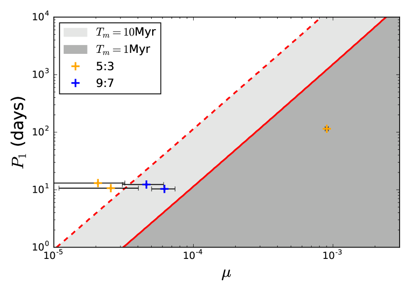
Figure 7: Estimation for the region in the $(\mu,P_{1})$ parameter space where resonance capture is possible. Here $\mu=\mu_{1}+\mu_{2}=(m_{1}+m_{2})/M_{\star}$ and $P_{1}$ is the orbital period of the inner planet. In the dark (light) grey regions, the system can be captured for $T_{m}=1$ Myr ($10$ Myr), with the solid (dashed) line showing the boundary [the second inequality of (45)]. The crosses mark the five known systems that are close to (i.e. with period ratio deviation less than $6\times 10^{-3}$) the second-order MMR; the color of the marker labels different MMR, as indicated, and the error bars mark the uncertainty of $\mu$. All these systems lie inside or close to the estimated resonance capture region.

5 Resonance of Two Planets of Comparable Masses

There are two motivations to study second-order MMR involving two similar mass planets. First, our analysis of the restricted three-body problem (Sections 2 and 3) shows that the stability property of the equilibrium following resonance capture is completely different in the two limiting cases ($m_{1}\ll m_{2}$ and $m_{2}\ll m_{1}$). It is necessary to know where the transition between the two behaviors (stable vs overstable equilibrium state) occurs, and whether the values of $T_{e}$ and $T_{m}$ affect the stability. Second, four of the five observed planet pairs close to second-order resonances have mass ratio close to unity, so a model for similar mass planets in resonance is necessary if we want to compare our theoretical result with observations.

Previous studies (Delisle et al., 2014, 2015) calculate the stability of the captured state for two planets with general mass ratio using an integrable Hamiltonian. This Hamiltonian is exact in the two limiting cases ($m_{1}\ll m_{2}$ and $m_{2}\ll m_{1}$), but is approximate for planets with comparable masses. In this section we first derive the full non-integrable resonance Hamiltonian for the general ($m_{1}\sim m_{2}$) case, and study the mechanism of resonance capture by analyzing the fixed points of the system. Then we obtain the conditions for resonance capture, and compare these with our results for the limiting cases. Finally we calculate how the stability and escape time (i.e. time inside resonance before escaping, when the capture is unstable) depends on $T_{m}$ and $T_{e}$, and compare the results with Delisle et al. (2015). Due to the complexity of algebra, we omit most of the calculation in the main text, and relegate the details to Appendix A (available online).

5.1 Hamiltonian and fixed points

For first-order resonances, the Hamiltonian of planets with comparable masses can be transformed to that of a one degree of freedom system, of the same form as the restricted problem (Sessin & Ferraz-Mello, 1984; Wisdom, 1986; Henrard et al., 1986; Deck et al., 2013). However, such simplification is impossible for second-order resonances. This is because the leading terms of the resonant and secular perturbations have similar strengths, and the “mixing” of the two perturbations obstruct simplification. Delisle et al. (2014) propose a method to reduce the Hamiltonian of an arbitrary order MMR to an integrable form which has the same mathematical form as the Hamiltonian in the limiting cases, but this reduction involves nontrivial approximation for second and higher order MMRs. Here, in order to better compare the capture mechanism with the limiting cases and give more accurate results, we choose to use the non-integrable Hamiltonian. A thorough study of the phase space topology is difficult; nevertheless, we can gain considerable insight into the resonant motion of the two planets by analyzing the fixed points of the Hamiltonian.

For two planets with comparable masses in a second-order MMR, the Hamiltonian can be simplified to that of a two degree of freedom system (see Appendix A)

$$\begin{split}-H=&(x_{1}^{2}+x_{2}^{2}+y_{1}^{2}+y_{2}^{2}+\eta)^{2}+(Ax_{1}+Bx_{2})^{2}\\ &+(Cy_{1}+Dy_{2})^{2}+E^{2}x_{1}^{2},\end{split}$$ (46)

where the canonical momentum and coordinate pairs $(x_{1},y_{1})$ and $(x_{2},y_{2})$ are defined by (for $e_{i}\ll 1$)

$$x_{1}=\sqrt{2\Theta_{1}}\cos\theta_{1},~{}~{}~{}y_{1}=\sqrt{2\Theta_{1}}\sin\theta_{1},$$ (47)

$$x_{2}=\sqrt{2\Theta_{2}}\cos\theta_{2},~{}~{}~{}y_{2}=\sqrt{2\Theta_{2}}\sin\theta_{2},$$ (48)

with

$$\begin{split}\Theta_{1}=\frac{1}{2}\mu_{2}^{-1}\alpha_{\rm res}^{1/2}e_{1}^{2},~{}~{}~{}\Theta_{2}=\frac{1}{2}\mu_{1}^{-1}e_{2}^{2},\end{split}$$ (49)

where $\alpha_{\rm res}\equiv[(j-2)/j]^{2/3}$. The resonant angles $\theta_{1},\theta_{2}$ are

$$\theta_{1}=\frac{j}{2}\lambda_{2}-\frac{(j-2)}{2}\lambda_{1}-\varpi_{1},$$ (50)

$$\theta_{2}=\frac{j}{2}\lambda_{2}-\frac{(j-2)}{2}\lambda_{1}-\varpi_{2}.$$ (51)

The parameter $\eta$ is a constant in the absence of dissipation, and is related to $\alpha=a_{1}/a_{2},e_{1}$ and $e_{2}$ by

$$\begin{split}\eta=&\frac{4}{j\mu_{0}}\left[1-\left(\frac{\alpha}{\alpha_{\rm res}}\right)^{1/2}\right]-\mu_{2}^{-1}\alpha_{\rm res}^{1/2}e_{1}^{2}\\ &-\mu_{1}^{-1}e_{2}^{2}+\text{constant of $\mathcal{O}(1)$},\end{split}$$ (52)

where

$$\begin{split}\mu_{0}\equiv\mu_{1}+\mu_{2}\alpha_{\rm res}\end{split}$$ (53)

is an “effective total mass ratio” that will frequently appear in this section, and the $\mathcal{O}(1)$ constant can be solved numerically (see Appendix A). Note that the last term in Eq. (52) trivially shifts the location of the resonance, with the shift in resonant $\alpha$ being of order $\mu_{0}$. For the Hamiltonian (46), time is normalized by

$$\begin{split}\tau=t/T_{0},~{}~{}~{}T_{0}\equiv\left(\frac{3j^{2}}{32}\mu_{0}n_{2}\right)^{-1}\sim\mu_{0}^{-1}P_{1}.\end{split}$$ (54)

The parameters $A,B,C,D,E$ are all real, and they only depend on $j$ and the mass ratio

$$\begin{split}q\equiv m_{1}/m_{2}.\end{split}$$ (55)

For $q\sim 1$, these parameters are all of order unity. The full derivation of the Hamiltonian can be found in Appendix A.

The phase space now have 4 dimensions, so we cannot conveniently plot the phase space topology as we did for the restricted problem in Sections 2-3. Instead, we analyze the fixed points of the system, which are informative enough to illustrate the resonance capture mechanism. The coordinates of the fixed points can be calculated by solving $d(x_{1},x_{2},y_{1},y_{2})/d\tau=0$ (see Appendix A). The system can have $1,3,5,7$ or $9$ fixed points. There is always a fixed point that lies in the origin (labeled as FP₀), and all other fixed points come in pairs [i.e. if $(x_{10},x_{20},y_{10},y_{20})$ is a fixed point, then $(-x_{10},-x_{20},-y_{10},-y_{20})$ is also a fixed point, and their properties are identical]. These fixed points have the form:

$${\rm FP}_{1}:~{}~{}~{}(0,0,\pm y_{11}\sqrt{-\eta},\pm y_{21}\sqrt{-\eta})$$ (56)

$${\rm FP}_{2}:~{}~{}~{}(0,0,\pm y_{12}\sqrt{-\eta+\eta_{2}},\mp y_{22}\sqrt{-\eta+\eta_{2}})$$ (57)

$${\rm FP}_{3}:~{}~{}~{}(\pm x_{11}\sqrt{-\eta+\eta_{3}},\pm x_{21}\sqrt{-\eta+\eta_{3}},0,0)$$ (58)

$${\rm FP}_{4}:~{}~{}~{}(\pm x_{12}\sqrt{-\eta+\eta_{4}},\pm x_{22}\sqrt{-\eta+\eta_{4}},0,0)$$ (59)

where the parameters $\eta_{2,3,4}$ and $x_{ij}$, $y_{ij}$ are functions of $A,B,C,D,E$, and

$$\begin{split}\eta_{4}<\eta_{2}<\eta_{3}<0,\end{split}$$ (60)

$$\begin{split}y_{11}^{2}+y_{21}^{2}=y_{12}^{2}+y_{22}^{2}=x_{11}^{2}+x_{21}^{2}=x_{12}^{2}+x_{22}^{2}=1.\end{split}$$ (61)

FP₁ exists only for $\eta<0$, and FP_i ($i=2,3,4$) only for $\eta<\eta_{i}$. Note that $\eta=\eta_{4}$ marks one boundary of the resonant region, while the other boundary is $\eta=0$. The $\eta$ value at which different fixed points “branch out” from the origin, and the distances of the fixed points from the origin, are summarized in Figure 8. Note that the (squared) distance is related to the planet’s eccentricities by

$$\begin{split}x_{1}^{2}+y_{1}^{2}+x_{2}^{2}+y_{2}^{2}=\mu_{2}^{-1}\alpha_{\rm res}^{1/2}e_{1}^{2}+\mu_{1}^{-1}e_{2}^{2}.\end{split}$$ (62)

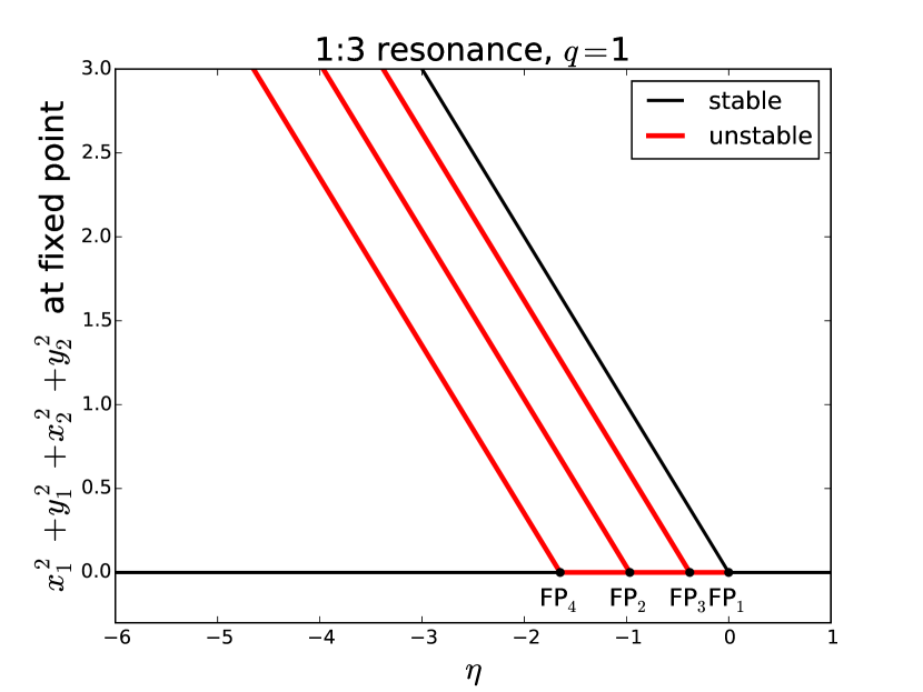
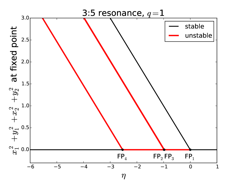
Figure 8: Locations of fixed points for 1:3 and 3:5 resonance with equal mass planets ($m_{1}=m_{2}$). The vertical axis shows the (squared) distance between the fixed point and the origin (Eq. 62). The four pairs of fixed points other than the origin (FP₀) are labeled by ${\rm FP}_{1}$ - ${\rm FP}_{4}$. Note that each branch of FP_i corresponds to two fixed points; and all fixed points move away from the origin along different directions as $\eta$ decreases. The stability of the fixed points are marked by color; red intervals are unstable. We see that the stability for each branch of fixed points and the distribution of branching points are qualitatively the same, except that for the 3:5 resonance the branching points of FP₂ and FP₃ are much closer. Results for resonances with larger $j$ (e.g. 5:7, 7:9) and other mass ratios are qualitatively the same. Note that the distribution of the stable fixed points is very similar to that in Figure 3.

The stability of fixed points FP₁ is manifest, since they are local maxima of the Hamiltonian. Also, FP₀ is stable when the system is away from resonance ($\eta<\eta_{4}$ or $\eta>0$), since it is clearly an extremum of the Hamiltonian when $|\eta|\gg 1$. In general, the stability of a fixed point can be determined by calculating the eigenvalues of the linearized equations of motion (similar to the stability analysis for Section 2.4 and 3.3, except that the system is non-dissipative); a fixed point is stable only when all eigenvalues have zero real part. We numerically computed the eigenvalues for each fixed point, and the result is shown in Figure 8. It turns out that FP₂, FP₃ and FP₄ are unstable; and FP₀ is unstable when $\eta\in(\eta_{4},0)$. The fixed point FP₁ is always stable.

Comparing Figure 8 with Figure 3 shows that the locations of the stable fixed points for $q\sim 1$ are qualitatively the same as in the limiting mass ratio cases, while extra branches of unstable fixed points exist for $q\sim 1$. Therefore, the mechanism of resonance capture and eccentricity excitation should be mostly similar:

(i) For slowly increasing $\eta$, the eccentricities of the planets suddenly increase as the origin becomes unstable at $\eta=\eta_{4}$; after that the eccentricities remain approximately constant, conserving the phase space volume. The eccentricities can be excited to $\Theta_{1}\sim\Theta_{2}\sim 1$, and the system is not captured into resonance (both resonant angles are circulating).

(ii) For slowly decreasing $\eta$, the system tends to follow the stable fixed point, so it begins to advect with FP₁ as $\eta$ passes 0 and enters the resonant zone. The eccentricities keep growing with decreasing $\eta$; the system may reach an equilibrium if $\eta$ becomes constant due to the dissipative effect associated with planet-disk interaction.

5.2 Capture mechanism and condition

To examine the effect of planet migration we need to consider $d\eta/dt$. Using Eqs. (8), (9) and (52), we have

$$\begin{split}\frac{d\eta}{dt}=&-\frac{2}{j\mu_{0}}\left(T_{m,2}^{-1}-T_{m,1}^{-1}\right)\\ &+2T_{e,1}^{-1}\Theta_{1}\left[1+\frac{p_{1}}{(j-2)(1+\alpha_{\rm res}^{-1}q)}\right]\\ &+2T_{e,2}^{-1}\Theta_{2}\left[1-\frac{p_{2}}{j(1+\alpha_{\rm res}q^{-1})}\right].\end{split}$$ (63)

For the following calculation, we will assume $p_{1}=p_{2}=2$. The equations of motion for $x_{i},y_{i}$ can be obtained by adding dissipative terms to the non-dissipative equations [derived from the Hamiltonian (46)] for $dx_{i}/d\tau$ and $dy_{i}/d\tau$. These dissipative terms are

$$\begin{split}\left.\frac{dx_{i}}{d\tau}\right|_{\rm diss}=-\frac{x_{i}}{\tau_{e,i}},~{}~{}~{}\left.\frac{dy_{i}}{d\tau}\right|_{\rm diss}=-\frac{y_{i}}{\tau_{e,i}}.\end{split}$$ (64)

Resonant capture requires $d\eta/d\tau<0$ (see the last paragraph of Section 5.1). Thus a necessary condition for capture is

$$\begin{split}T_{m}\equiv\frac{1}{T_{m,2}^{-1}-T_{m,1}^{-1}}>0.\end{split}$$ (65)

In other words, resonance capture always requires convergent migration, in agreement with the limiting mass cases. When the eccentricities of the planets are excited due to the decrease of $\eta$, the increased eccentricities tend to increase $\eta$ because the last two terms in Eq. (63) are always positive. Therefore, there exists an equilibrium state where the decrease of $\eta$ due to convergent migration is balanced by the increase of $\eta$ due to excited eccentricities. The system can be held at this equilibrium state permanently if small oscillations about the equilibrium point is stable (see Fig. 9). When the equilibrium point is overstable, the system will eventually leave the libration zone. In this case, the system exhibits two possible outcomes, depending on $\eta_{\rm eq}$ (the value of $\eta$ at the equilibrium state): For $\eta_{\rm eq}<\eta_{4}$ ($\sim-1$; see Fig. 8), the system escapes from the resonance, and the period ratio increasingly deviates from the resonant value (Fig. 10); for $\eta_{\rm eq}>\eta_{4}$, the system eventually enters a quasi-equilibrium state, where the resonant angles circulate but the period ratio stays approximately constant and the eccentricities undergo oscillations (see Fig. 11). The stability criterion of the equilibrium state following resonance capture is discussed in Section 5.4.

Comparing these results with the two limiting cases ($q\ll 1,q\gg 1$) shows that the mechanism of resonance capture is qualitatively the same: The systems starts with small eccentricities; as $\eta$ decreases and passes 0, the system advects with (one of) FP₁ because the origin is no longer stable; further evolution of the system after capture depends on the “location” ($\eta_{\rm eq}$) and stability of the equilibrium state. We expect that the requirement on $T_{e}$ and $T_{m}$ for resonance capture should be similar to the limiting cases: For $T_{e}$, we require

$$\begin{split}T_{e,i}\gtrsim T_{0}.\end{split}$$ (66)

Note that the system can still be captured into resonance if one of $T_{e,i}$ ($i=1,2$) is too small to allow excitation of $e_{i}$; in this case only the eccentricity of the other planet is excited and only that planet’s resonant angle is librating upon capture. Similar to Eq. (44), the requirement on $T_{m}$ is

$$\begin{split}T_{m}\gtrsim\mu_{0}^{-1}T_{0}|\ln\Theta_{i,0}|,\end{split}$$ (67)

where $\Theta_{i,0}$ is the initial (prior to entering the resonance) value of $\Theta_{i}$.

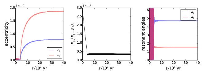
Figure 9: Stable capture of similar mass planets into 3:5 MMR. The system has $M_{\star}=1M_{\odot},~{}~{}m_{1}=10M_{\oplus},~{}~{}m_{2}=5M_{\oplus},~{}~{}a_{1}=0.1AU,~{}~{}T_{m,1}=4\,{\rm Myr},~{}~{}T_{m,2}=2\,{\rm Myr}$, and $T_{e}=10\,{\rm kyr}$. We see that the eccentricities of both planets are excited, and the period ratio, eccentricities and resonant angles all converge to constants. The two resonant angles are at $\theta_{1}=\pi/2$ and $\theta_{2}=3\pi/2$. Note that another final state with $\theta_{1}$ and $\theta_{2}$ switched is equally likely to occur.

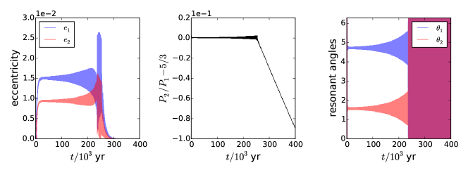
Figure 10: Capture of similar mass planets into 3:5 MMR followed by escape from the resonance (overstable equilibrium with $\eta_{\rm eq}<\eta_{4}$). The system is the same as that in Fig. 9, except $m_{1}=5M_{\oplus}$ and $m_{2}=10M_{\oplus}$. We see that after reaching the equilibrium state, the libration amplitudes of resonant angles increase due to overstability and the system escapes from resonance eventually.

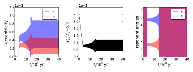
Figure 11: Capture of similar mass planets into 3:5 MMR followed by “partial” escape (overstable equilibrium with $\eta_{\rm eq}>\eta_{4}$). The system is the same as that in Fig. 10, except $T_{e}=1~{}{\rm kyr}$. The libration around equilibrium is still overstable, but the system ends up in a stable circulating orbit with the period ratio oscillating around a constant value.

5.3 Effect of large initial eccentricities

So far in this section we have assumed that the initial eccentricities of the two planets are small ($\Theta_{1,0}\sim e_{1,0}^{2}/\mu_{2}\lesssim 1$ and $\Theta_{2,0}\sim e_{2,0}^{2}/\mu_{1}\lesssim 1$). This assumption is in general satisfied for small planets because their eccentricities can be quickly damped by the disk. In systems consisting of a massive planet and a very small planet, the dimensionless eccentricity parameter ($\Theta$) of the big planet is inversely proportional to the smaller planet’s mass and can become large even when the physical eccentricity is small. Here we consider the effect when one or both planets have $\Theta_{i,0}\gtrsim 1$.

As noted in Section 4, for the restricted three-body problem, resonance trapping becomes probabilistic when $\Theta_{0}\gtrsim 1$ even for very large (infinite) $T_{e}$ and $T_{m}$. For systems with comparable mass planets, we can similarly conjecture that trapping becomes probabilistic if $\Theta_{1,0}$ or $\Theta_{2,0}$ is $\gtrsim 1$. This is because when the initial $\Theta_{1}$ or $\Theta_{2}$ is $\gtrsim 1$, the system cannot settle near the stable fixed point FP₁ before the origin (FP₀) becomes stable again, and resonance trapping should be probabilistic. Numerical integration of the equations of motion when one or both planets have initial $\Theta_{i}\gtrsim 1$ confirms this conjecture.

This line of reasoning does not fully apply to systems with relatively large mass ratio ($q$ or $q^{-1}\gtrsim 5$). For such systems, the perturbation on the larger planet from the smaller one is much weaker than the perturbation on the smaller planet from the larger one; therefore the evolution of the small planet’s eccentricity is barely affected by the other planet’s eccentricity. Thus, if the smaller planet has a large initial $\Theta$, it cannot be captured into resonance. However, when only the larger planet has initial $\Theta\gtrsim 1$, the small planet can still be captured into resonance; in this case the small planet attains an excited eccentricity and its corresponding resonant angle librates, while the larger planet’s eccentricity is not excited, and its resonant angle circulates (see Sections 2-4).

5.4 Stability of capture and escape from resonance

As discussed in Section 5.2, after resonance capture, the system approaches an equilibrium in which eccentricity excitation due to resonant forcing balances eccentricity damping due to planet-disk interaction. Further evolution of the system depends on the location of the equilibrium and its stability. In particular, if the equilibrium is overstable, the system will completely escape from the resonance if $\eta_{\rm eq}<\eta_{4}\sim-1$, where $\eta_{\rm eq}$ is the value of $\eta$ in the equilibrium state. The equilibrium state can be determined by setting $dx_{i}/d\tau=dy_{i}/d\tau=0$ (including the dissipative terms) and $d\eta/d\tau=0$ [see Eq. (63)]. In orders of magnitude, we find

$$\begin{split}|\eta_{\rm eq}|\sim\frac{T_{m,2}^{-1}-T_{m,1}^{-1}}{\mu_{0}(T_{e,1}^{-1}+T_{e,2}^{-1})},\end{split}$$ (68)

and when $q\sim 1$,

$$\begin{split}\Theta_{1,\rm eq}\sim\Theta_{2,\rm eq}\sim|\eta_{\rm eq}|.\end{split}$$ (69)

The resonant angles are $\theta_{1}\simeq\pm\pi/2$ and $\theta_{2}\simeq\mp\pi/2$.

Based on the results of the restricted three-body problems (Sections 2-3), we expect resonance capture (equilibrium) to be stable when $q\equiv m_{1}/m_{2}\gtrsim 1$, and overstable when $q\lesssim 1$. Here we provide a more accurate determination of the critical $q=q_{\rm crit}$ at which the transition from stability to overstability occurs, in order to predict the overall population of planet pairs in second-order resonances as a result of convergent migration. Note that we only examine capturing into the equilibrium state where both resonant angles librate. Capture into resonance with one librating resonant angle (e.g. the $q\to 0$ or $\infty$ limiting cases) or capture with no librating resonant angle (i.e. when the equilibrium point is unstable but $\eta_{\rm eq}\gtrsim\eta_{4}$) are not considered.

To determine the stability of resonance capture, we linearize the equations of motion (with dissipation) near the equilibrium point and calculate the eigenvalue $\lambda$. For an overstable system, the escape timescale from the resonance is

$$\begin{split}\tau_{\rm esc}\sim 1/\lambda_{r}~{}~{}~{}(\text{when }\lambda_{r}>0)\end{split}$$ (70)

where $\lambda_{r}$ is the maximum real part of the eigenvalues.

Because of the complexity of the system, we cannot obtain a simple analytical expression for $\lambda_{r}$ as we did for the restricted three-body problems (Sections 2-3); instead, we solve the eigenvalue problem numerically to calculate $\tau_{\rm esc}$ for various parameters. The system is fully specified by the parameters $\tau_{e,i},\tau_{m},\mu_{i},n_{1},j$ and $q$. From the dimensionless form of the equations of motion we see that all factors of $n_{1}$ cancel out, and $\mu_{i}$ and $\tau_{m}$ only appear in the combination $\mu_{0}\tau_{m}$ (see Appendix A). For clarity, we use

$$\begin{split}\tau_{e}\equiv\sqrt{\tau_{e,1}\tau_{e,2}},~{}~{}~{}q_{e}=\tau_{e,2}/\tau_{e,1}\end{split}$$ (71)

instead of $\tau_{e,i}$. Note that $q_{e}$ is the ratio of the eccentricity damping rates. In general, we find that $\tau_{\rm esc}$ depends very weakly on $\mu_{0}\tau_{m}$, as long as $\mu_{0}\tau_{m}\lesssim\tau_{e}$, in agreement with the results of the restricted problem. Thus, we only need to consider the dependence of $\tau_{\rm esc}$ on $\tau_{e},q_{e},j$ and $q$.

Figure 12 shows $\tau_{\rm esc}=\lambda_{r}^{-1}$ for the 3:5 MMR as a function of $q$ for different values of $q_{e}$ and $\tau_{e}$. We see that $\tau_{\rm esc}/\tau_{e}$ depends weakly on $\tau_{e}$ (similar to the behavior of the restricted problem). In general, $\tau_{\rm esc}/\tau_{e}$ decreases with increasing $q_{e}$, while the critical $q_{\rm crit}$ increases with $q_{e}$. Thus, for a given MMR (given $j$), the stability of the equilibrium mainly depends on $q$ and $q_{e}$. Figure 13 shows this dependence for different resonances. Empirically, we find that the critical mass ratio (above which the equilibrium state is stable) is given by

$$q_{\rm crit}\simeq 2q_{e}^{2/3}$$ for 1:3 resonance, (72)

$$q_{\rm cirt}\simeq q_{e}^{1/2}$$ for other resonances. (73)

The result for the 1:3 MMR is different because the corresponding $\alpha_{\rm res}$ is much smaller than that of the other resonances, and there is an “indirect term” (see Murray & Dermott 1999) that only appears in the 1:3 MMR. We see that for most of the unstable region in the $q-q_{e}$ parameter space, $\tau_{\rm esc}$ is close to $\tau_{e}$. Near the stability limit, $\tau_{\rm esc}$ is significantly larger than $\tau_{e}$. For $q\lesssim 1$, we find that $\tau_{\rm esc}\sim\tau_{e,1}$.

Delisle et al. (2015) gives the stability critarion in terms of the equilibrium eccentricity ratio; the captured state is stable if $q_{e}^{-1}\gtrsim(e_{1,\rm eq}/e_{2,\rm eq})^{2}$. Figure 14 shows the eccentricity ratio at the captured equilibrium state, which we have analytically calculated using the location of the fixed point FP₁. We see that for all second-order MMRs except the 1:3 MMR, $e_{1,\rm eq}/e_{2,\rm eq}\simeq q^{-1}$; for 1:3 MMR $e_{1,\rm eq}/e_{2,\rm eq}$ has a different dependence on $q$ around $q\sim 1$. This explains why our stability boundary (72) is different only for the 1:3 MMR. For second-order MMRs other than the 1:3 MMR, the criterion in Delisle et al. (2015) suggests that capture is stable for $q_{e}\lesssim q^{2}$, agreeing with our equation (73). Figure 13 compares $q_{\rm crit}$ obtained using the criterion of Delisle et al. (2015) with our result; we see that the two results are very similar when the relationship between the eccentricity ratio and mass ratio (Figure 14) is spelled out.

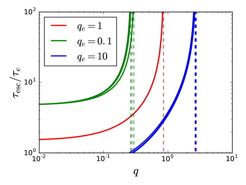
Figure 12: Resonance escape time $\tau_{\rm esc}$ (in units of $\tau_{e}$, the eccentricity damping time) for the 3:5 MMR as a function of $q=m_{1}/m_{2}$ for different $\tau_{e}$ and $q_{e}=\tau_{e,2}/\tau_{e,1}$, with given $\mu_{0}\tau_{m}=10$. Different colors mark different $q_{e}$; for each $q_{e}$ there are three curves for $\tau_{e}=100,300$ and $1000$. The curves are calculated using $\mu_{0}\tau_{m}=100$, although the results are unchanged for other values of $\mu_{0}\tau_{m}\lesssim\tau_{e}$. We see that for each $q_{e}$, the difference between the three curves are very small, suggesting that $\tau_{\rm esc}/\tau_{e}$ barely depends on $\tau_{e}$. In general $\tau_{\rm esc}/\tau_{e}$ is smaller for larger $q_{e}$, but $q_{\rm crit}$ is larger. Other resonances show similar trends.

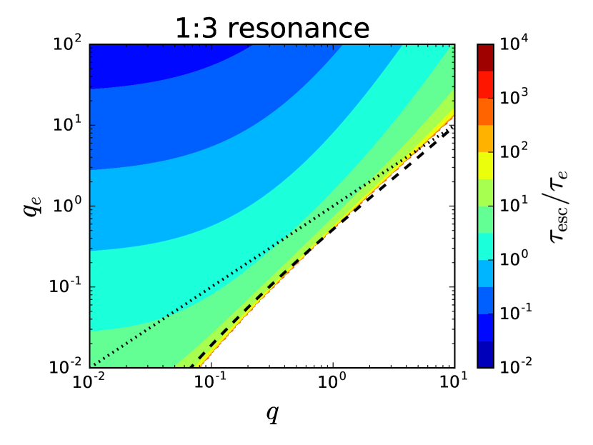
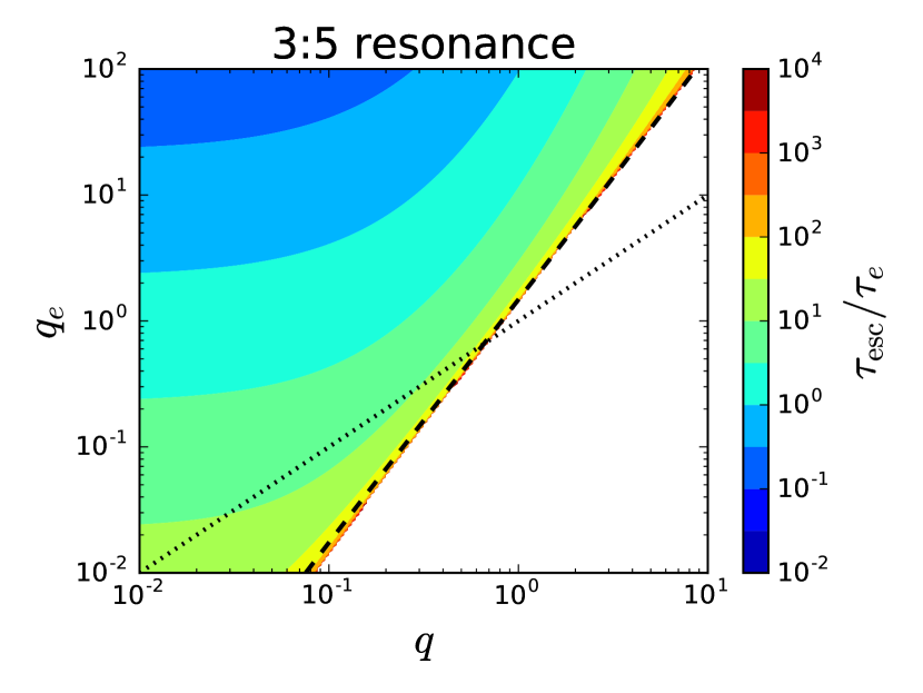
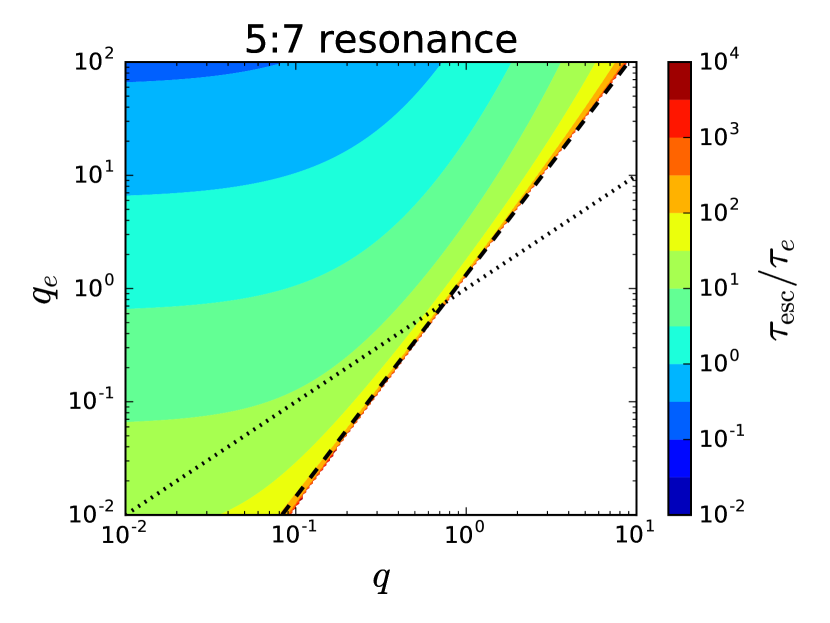
Figure 13: Resonance escape time $\tau_{\rm esc}$ for the 1:3, 3:5 and 5:7 MMRs as a function of $q=m_{1}/m_{2}$ and $q_{e}=\tau_{e,2}/\tau_{e,1}$. The results are obtained using the values $\mu_{0}\tau_{m}=10$ and $\tau_{e}=1000$, although the results are nearly unchanged for other values as long as $\mu_{0}\tau_{m}\lesssim\tau_{e}$. Color shows the value of $\tau_{\rm esc}/\tau_{e}$, while the white region corresponds to stability (infinite escape time). Note that the behavior of the 3:5 and 5:7 resonances are very similar, while for the 1:3 resonance the overstable region is larger. The stability limit is approximately $q_{\rm crit}\simeq q_{e}^{1/2}$ for the 3:5 and 5:7 resonances, and $q_{\rm crit}\simeq 2q_{e}^{2/3}$ for the 1:3 resonance. The black dashed line shows the stability boundary using the criterion of Delisle et al. (2015) (and using the relationship between the eccentricity ratio and mass ratio as depicted in Figure 14), which agrees with our result. The black dotted line shows $q_{e}=q$; systems with low-mass planets in a gaseous disk should lie close to this line. For such systems, $q_{\rm crit}$ for the 3:5 or 5:7 resonance is smaller than that for the 1:3 resonance.

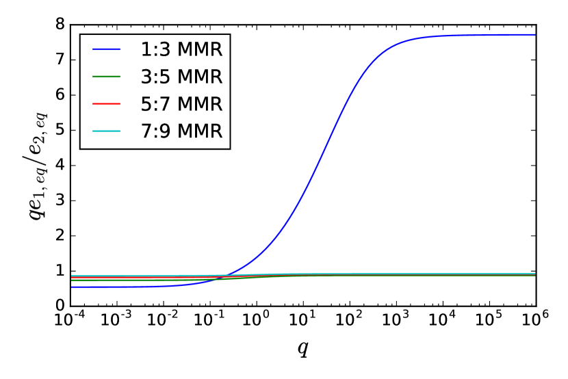
Figure 14: Ratio of the two planets’ eccentricities at the equilibrium state (the fixed point FP₁) as a function of the mass ratio $q$. For $q\ll 1$ and $q\gg 1$, $qe_{1,\rm eq}/e_{2,\rm eq}$ is nearly independent of $q$. For $q\sim 1$, $qe_{1,\rm eq}/e_{2,\rm eq}$ grows significantly as $q$ increases for the 1:3 MMR and is nearly constant for the other second-order MMRs. This explains the difference between equations (72) and (73).

For realistic systems with relatively small (non-gap-opening) planets, we have [see Eq. (11)]

$$\begin{split}\frac{q_{e}}{q}\sim\frac{F(a_{1})}{F(a_{2})}~{}~{}\text{with}~{}~{}F(a)\equiv\Sigma_{d}a^{4.5}h^{-4},\end{split}$$ (74)

where $\Sigma_{d}$ and $h$ are surface density and scale height of the disk. Since the two planets in resonance are relatively close to each other, we expect this ratio to be close to 1. Therefore, the system should lie near the black dashed line in Figure 13. From this figure we see that for systems with $q_{e}=q$, $q_{\rm crit}$ is slightly below 1 for the 3:5 and 5:7 resonances, and about 5 for the 1:3 resonance. This means that a system undergoing convergent migration (which usually implies $q,q_{e}\lesssim 1$) is unlikely to be stably captured into the 1:3 resonance, while stable capture into the 3:5 or 5:7 resonance is possible.

Note that $q_{\rm crit}$ is sensitive to the physical property of the disk, especially for the 1:3 resonance. For disks with $F(a_{1})>F(a_{2})$, we expect $q_{e}/q>1$, and $q_{\rm crit}$ is shifted to larger values (compared to that depicted on Figure 13); for disks with $F(a_{1})<F(a_{2})$, $q_{\rm crit}$ is shifted to smaller values. Using Eqs. (74) and (72)-(73), we find $q_{\rm crit}\simeq 8[F(a_{1})/F(a_{2})]^{2}$ for the 1:3 resonance and $q_{\rm cirt}\simeq F(a_{1})/F(a_{2})$ for the other resonances. Also recall that convergent migration requires $T_{m,1}^{-1}<T_{m,2}^{-1}$, which implies $q\lesssim(\Sigma_{d}a^{2.5}h^{-2})_{2}/(\Sigma_{d}a^{2.5}h^{-2})_{1}$ using Eq. (10). This again suggests that the stable capture into the 1:3 resonance during convergent migration is unlikely.

We end this section by emphasizing that, even for an overstable equilibrium, the resonance escape time $T_{\rm esc}=\tau_{\rm esc}T_{0}$ can be much larger than the eccentricity damping time $T_{e,i}$ when the mass ratio is close to the stability boundary $q_{\rm crit}$. Thus, a nontrivial portion of such systems may stay close to resonance until migration ends, even when $T_{e,i}$ is much smaller than the disk lifetime. Figure 15 gives an example for the 3:5 resonance.

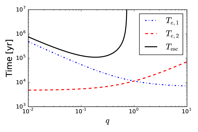
Figure 15: Resonance escape timescale $T_{\rm esc}$ as a function of $q=m_{1}/m_{2}$ for a system with $m_{1}+m_{2}=15M_{\oplus}$, $M_{\star}=1M_{\odot}$, and $T_{e,i}=(M_{\oplus}/m_{i})10^{5}\,{\rm yr}$. In this calculation we consider $j=5$ (the 3:5 resonance) and $T_{m}=1$ Myr, although the result is not sensitive to these parameters. The eccentricity damping time $T_{e,i}$ is also shown for reference. We see that $T_{\rm esc}\gtrsim T_{e,i}$ for all values of $q$, and near $q_{\rm crit}$ the difference between $T_{e,i}$ and $T_{\rm esc}$ becomes significant.

6 N-Body Simulations

In the previous sections, we have studied the dynamics of a two-planet system near resonance analytically using a Hamiltonian formalism. N-body calculations can be used to verify the results obtained from this Hamiltonian approach. More importantly, N-body calculations are necessary in order to study the migration of planet between resonances and compare the timescales the planets spend inside and outside the resonance.

In this section, we use the MERCURY code (Chambers, 1999) to integrate the evolution of a two-planet system, with planet-disk interaction modeled by adding an extra force on each planet (e.g., Snellgrove et al. 2001; Nelson & Papaloizou 2002; Lee & Peale 2002)

$$\begin{split}\left.\frac{d\mathbf{v}_{i}}{dt}\right|_{\rm disk}=-\frac{2\dot{\mathbf{r}}_{i}\cdot\hat{\mathbf{r}}_{i}}{T_{e,i}}\hat{\mathbf{r}}_{i}-\frac{\dot{\mathbf{r}}_{i}\cdot\hat{\boldsymbol{\varphi}}_{i}}{2T_{m,i}}\hat{\boldsymbol{\varphi}}_{i},\end{split}$$ (75)

where $\hat{\mathbf{r}}_{i}$ and $\hat{\boldsymbol{\varphi}}_{i}$ are the unit vectors in radial and azimuthal directions, $T_{e,i}$ and $T_{m,i}$ are the eccentricity damping and migration timescales as previously defined [Eqs. (8)-(9)], and this model of planet-disk interaction corresponds to $p_{i}=2$. We always use $e_{1}=e_{2}=0$ as the initial condition far from resonance. Non-resonant interaction between the planets could excite finite eccentricities before entering resonance to allow capture.

6.1 Stable resonance capture of similar mass planets

First we use N-body integrations to test the validity of our analytical results for the case of stable resonance capture. Figure 16 shows the evolution of a system with the same parameter as in Figure 9. Note that in our $N$-body integrations, we have chosen the initial condition (initial $\alpha=a_{1}/a_{2}$) further away from resonance (than in Fig. 9) in order not to miss any nontrivial behavior of the system before entering the resonance. We see that the evolution of the system agrees with our previous results. In particular, the equilibrium eccentricities of the planets and the equilibrium $\eta$ match the analytical prediction very well. We conclude that our analytical Hamiltonian approach captures the relevant dynamics of the resonance when the eccentricities of the planets are not too large.

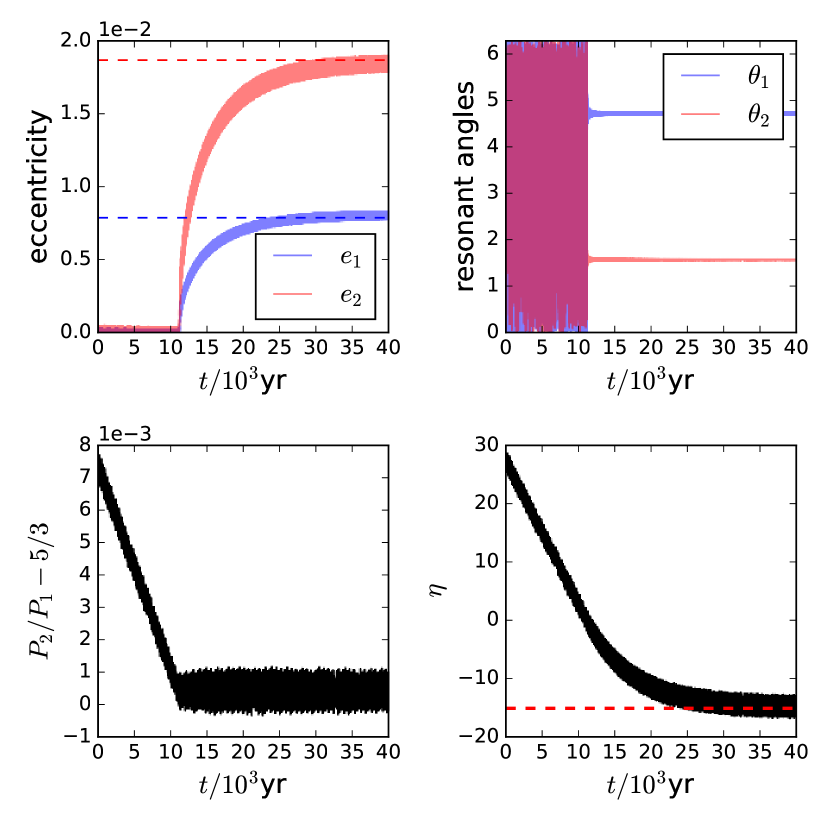
Figure 16: $N$-body simulation of capture into the 3:5 MMR of a system with the same parameters as in Figure 9. In the upper left panel, the analytical prediction of the final planet eccentricity (see Appendix A for the calculation) is plotted as blue/red-dashed line. In the lower right panel, the analytical prediction of the final (equilibrium) $\eta$ is shown as red-dashed line. These analytical results agree with the N-body results very well; the qualitative behaviors of the resonance angles (upper right panel) and period ratio (lower left panel) also match those in Figure 9.

It is worth noting that the system we choose for Figure 16 has a similar total planet mass and semi-major axes as the five observed pairs of super Earths close to the second-order MMR (see Section 1). Further N-body examinations show that capture is still likely even when the planet masses are reduced to $m_{1}=m_{2}=2.5M_{\oplus}$ (while keeping the dissipation timescales at $T_{e}=10~{}{\rm kyr},T_{m,1}=4~{}{\rm Myr},T_{m,2}=2~{}{\rm Myr}$). This suggests that capture into second-order resonance should be common even for planets as small as several earth masses if the planets undergo convergent migration in a disk with migration time $T_{m,i}\gtrsim 1\,{\rm Myr}$.

6.2 Overstable resonance capture and escape

Next we consider the case of overstable resonance capture and the escape timescale from the resonance. Figure 17 shows the $N$-body simulation result for the evolution of a system with the same parameters as Figure 10. In Figure 10 we can already observe that the actual escape time from the 3:5 resonance (i.e. the length of time when the system is in resonance, in this case $\simeq 240\,{\rm kyr}$) is significantly longer than the eccentricity damping timescale ($T_{e}=10~{}{\rm kyr}$); this trend is also reflected in the estimation of $T_{\rm esc}$ based on eigenvalue of the linearized system (see Section 5.4), which gives $T_{\rm esc}\simeq 55\,{\rm kyr}$. Our $N$-body calculation (Fig. 17) also shows a large $T_{\rm esc}\simeq 140\,{\rm kyr}$ for the same system. The difference between the $N$-body result and the result of Figure 10 may come from the fact that in the $N$-body integration, the planets have larger eccentricities when entering the resonance. This difference may also come from the fact that our analytical estimation calculates $T_{\rm esc}$ based on the growth rate of libration amplitude for small libration around the fixed point; when the amplitude is larger the growth rate may be different. Thus, although our intuitive prediction that $T_{\rm esc}\sim T_{e}$ is roughly correct, the actual escape time $T_{\rm esc}$ is very often larger than $T_{e}$ by more than an order of magnitude. A direct consequence of this is that the system can spend relatively long time in resonance compared to the time between resonances even though $T_{e}\ll T_{m}$. For instance, in Figure 17 we see that the system spends roughly equal time in the 3:5 resonance and between the 3:5 and 2:3 resonances, while $T_{e}/T_{m}$ is only $1/400$. Thus, in the absence of other physical effects not considered in our analysis (see Section 7.2), we should expect more overstable systems in MMR than observed, since there is a nontrivial probability for such system to end its migration before exiting resonance. (Note that these systems become stable once the dissipative perturbations, i.e. migration torques, are gone.)

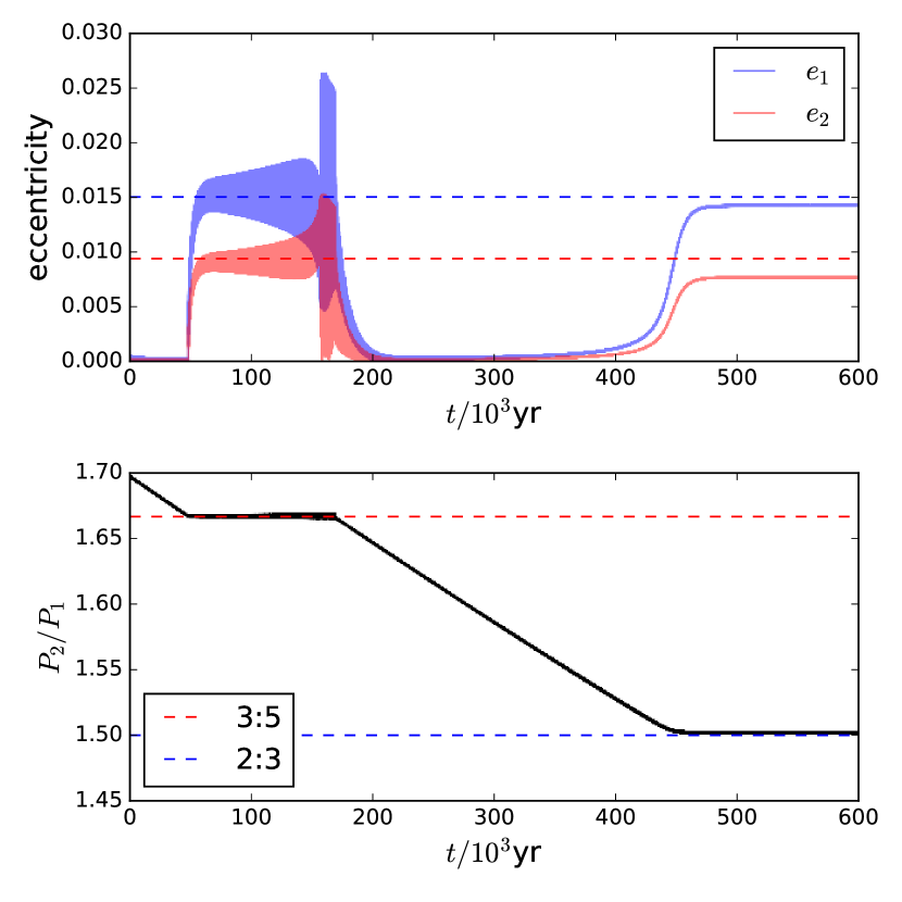
Figure 17: $N$-body simulation of capture into and escape from 3:5 MMR of a system with the same parameters as in Figure 10. In the eccentricity panel (left), the theoretical predictions of equilibrium eccentricities for the 3:5 MMR are plotted in blue/red-dashed lines. The system’s behavior qualitatively agrees with that in Figure 10, while the escape timescale differs by about a factor of 2; the difference may come from the fact that the actual system (i.e. the one in this figure) has a larger eccentricity when entering the resonance. After escaping from the 3:5 resonance, the system is subsequently captured into 2:3 mean motion resonance (this time the capture is stable). Note that the time the planet spends traveling between the two resonances is not much longer than the escape time.

7 Summary and Discussion

7.1 Summary of results

Motivated by the observations of Kepler multi-planet systems (see Section 1), we have carried out a theoretical study on the dynamics of second-order mean motion resonances (MMRs) for planets migrating in protoplanetary disks. In particular, we have examined the mechanism and the conditions of capturing the migrating planets into a second-order MMR, and studied the stability of the captured state, in order to determine whether and on what timescale the planets may escape from the resonance. We confirm our theoretical calculations with numerical $N$-body simulations. Our key results can be summarized as follows.

1. When one of the planets has a negligible mass compared to the other, the Hamiltonian of the planets near a second-order MMR can be reduced to that of a one degree of freedom system. In this limiting case (“restricted three-body problem”), the dynamics of MMR capture and its stability property can be explicitly calculated (Sections 2-3). When the planets have comparable masses, such simplification is no longer possible and the Hamiltonian has two degrees of freedom (Section 5). Nevertheless, the dynamics of MMR capture and the stability share similar features as the restricted three-body problem.

2. Planets can be captured into a second-order MMR only when the migration is convergent (Sections 2.2 and 5.2). For divergent migration, there is only a transient eccentricity excitation when the system passes the resonance, with the maximum eccentricity of the planet reaching $e_{1,2}\sim\sqrt{\mu_{2,1}}$ (where $\mu_{i}=m_{i}/M_{\star}$, and $m_{1,2}$ and $M_{\star}$ are the masses of the planets and the host star, respectively).

3. To capture the planets into a second-order MMR, the migration timescale $T_{m}$, the eccentricity damping timescale $T_{e}$ due to planet-disk interaction, and the initial (“pre-resonance”) eccentricity must satisfy Eq. (44). These conditions are distinct from those required for the first-order MMR capture (Appendix B, available online). When the migration timescale is shorter than that required by Eq. (44), the second-order resonance capture becomes probabilistic, and the capture probability decreases with decreasing $T_{m}$. In general, capture is easier for more massive planets and longer migration and eccentricity damping timescales. For planets in a disk with a migration timescale of $T_{m}\sim 1$ Myr, these conditions can be satisfied for super-Earths ($m_{i}\gtrsim$ a few $M_{\oplus}$) at $a\sim 0.1$ AU (see Fig. 7).

4. Following the resonance capture of the planets, an equilibrium state can be reached in which eccentricity excitation due to resonant planet-planet forcing balances eccentricity damping due to planet-disk interaction. However, this equilibrium may be overstable, leading to partial or permanent escape of the planets from the resonance. For the restricted three-body problem, we find that the captured equilibrium state is always overstable (with the growth time of order $T_{e}$) when $q\equiv m_{1}/m_{2}\ll 1$ ($q$ is the mass ratio of the inner and outer planets), and stable when $q\gg 1$ (Sections 2.4 and 3.3). For comparable mass planets, the stability of the equilibrium state depends not only on $q$, but also on the ratio of the eccentricity damping rate $q_{e}=T_{e,2}/T_{e,1}$ and the specific resonance (Section 5.4). Thus, in general, for planets captured into a second-order MMR, there are three possible outcomes:

   1. When $q\gtrsim q_{e}^{1/2}$ ($q\gtrsim 2q_{e}^{2/3}$ for 1:3 MMR), the planets are stably (permanently) captured with their period ratio held close to the resonance and the resonant angles librating (see Figs. 6, 9 and 16).

   2. When $q\lesssim q_{e}^{1/2}$ ($q\lesssim 2q_{e}^{2/3}$ for 1:3 MMR) and $|\eta_{\rm eq}|\lesssim 1$ [where $\eta_{\rm eq}$ is the value of the resonance parameter at the equilibrium; see Eq. (68) for a general estimate], the planets have circulating resonant angles but only partially escape from the resonance: the period ratio is still held close to and oscillate around the resonant value (see Figs. 2 and 11). Note that the second condition is met only when the planets are very massive ($\mu_{0}\gtrsim 10^{-2}$; see Eq. 53) or the difference between $T_{m,1}$ and $T_{m,2}$ is very small.

   3. When $q\lesssim q_{e}^{1/2}$ ($q\lesssim 2q_{e}^{2/3}$ for 1:3 MMR) and $|\eta_{\rm eq}|\gtrsim 1$, the planets escape from the resonance and the period ratio no longer stays close to the resonant value (see Figs. 5, 10 and 17).

   Delisle et al. (2015) have derived a criterion for stable capture in terms of the (equilibrium) eccentricity ratio of the planets. Our result agrees with theirs when the relationship between the eccentricity ratio and the mass ratio is spelled out (see Figure 14). Our calculation shows that in terms of $q$ and $q_{e}$, the criterion for stable capture for the 1:3 MMR is different from that for the other MMRs: The 1:3 resonance has a larger parameter space for unstable capture.

5. For planets that are captured but eventually leave the resonance, the linear growth time of the overstability is of order $T_{e}$, but can become much larger for systems near the stability threshold (see Figs. 12, 13 and 15). These analytical results and our $N$-body simulations both show that the escape time from resonance for these planets can be $10$-$100$ times larger than $T_{e}$. As a result, the time these planets spend in the resonance can be comparable to the time they spend migrating between resonances (Section 6.2 and Fig. 17).

7.2 Discussions

A major goal of this paper is to evaluate the probability of forming planet pairs in second-order MMRs by resonance capture during planet migration. There is a common preconception that capture into second-order MMRs is difficult because the planet perturbation associated with a second-order resonance may be too weak to counter the eccentricity damping due to planet-disk interaction. Our analysis of the conditions for capture indicates that capturing the planets into second-order MMRs is entirely possible, and only moderately large $T_{e}$ and $T_{m}$ are required. Therefore, a significant fraction of planets formed in gaseous disks could have been (permanently or temporarily) captured into second-order MMRs during migration. However, our analysis of the stability of the “captured” equilibrium shows that such capture is very often overstable: Following a capture, the system oscillates around the equilibrium state with growing amplitude, and eventually escapes from the resonance. For realistic systems, capture is stable [case 4(a) above] only when $q\gtrsim 1$, while convergent migration, which is necessary for capture in the first place, usually requires $q\lesssim 1$ for disk-driven Type I migration (see the end of Section 5.4 for discussion). We suggest that this is a likely reason why the observed period ratio distribution for Kepler multi-planet systems barely shows any peak near second-order MMRs (see Section 1). In particular, it is much more difficult to find a system stably captured into a second-order MMR than into a first-order MMR, because for first-order MMRs there is a large region in the parameter space where capture can be stable for $q\lesssim 1$ [see Appendix B and Deck & Batygin (2015)].

Our results can be used to explain some of the observed features of multi-planet systems in or near second-order MMRs, and comparison between our results and observations poses several interesting questions. As noted in Section 1, the Kepler sample currently contains at least five pairs of planets with period ratio within $7\times 10^{-3}$ of the exact resonance (and within $4\times 10^{-5}$ for two of the systems), and most of them are low-mass ($\sim 10M_{\oplus}$) planets, and have mass ratio $q\sim 1$. Our analysis suggests that it is indeed quite possible for these planets to be captured into resonance during migration, and the mass ratio could be explained by the fact that convergent migration and stable capture can be simultaneously satisfied only for $q\sim 1$. The low masses of these pairs could be explained by the fact that planets with larger masses and $q\sim 1$ captured into a second-order MMR can become dynamically unstable, especially for MMR with $j>5$ (such as $5:7$, $7:9$) [André & Papaloizou (2016) provide an example of such dynamical instability].

As noted before, the (de-biased) period ratio distribution of Kepler multi-planets exhibits no significant features near second-order MMRs except for the $3:5$ MMR [see Fig. 20 of Steffen & Hwang (2015)]. The overall paucity of planets in second-order MMRs (compared to those in first-order MMRs) can be explained by the fact that the captured planets in second-order MMRs are less stable. The fact that the $3:5$ MMR is more significant than the others could be caused by two effects: (i) For the $1:3$ MMR, the difference in stability criteria [see 4(a)-(c) in Section 7.1] implies that fewer planets can remain in this resonance compared to the 3:5 MMR; (ii) for resonances with $j>5$ (e.g. $5:7$, $7:9$), the planet’s spacing is so small that that few planets reach these resonances before being captured into another resonance or becoming dynamically unstable.

There are several factors we did not consider in this paper and they may impact the population of planets in second-order MMRs. First, the planet migration model we used assumes that migration is one-directional and the planet period ratio varies smoothly. Migration can shift from inward to outward (and sometimes convergent to divergent) as the disk evolves and disperses (e.g., Chatterjee & Ford 2015); this might move planets initially captured by convergent migration out of resonance. Second, waves and turbulences in protoplanetary disks may strongly affect second-order MMRs, since the resonant interaction is relatively weak. André & Papaloizou (2016) show that the waves in the disk produced by the planets do not affect capture into second-order MMR in some scenarios, while destabilizes the system in others. Third, we assumed that before migrating, the planets have accreted most of (at least a significant fraction of) their masses. It is possible that planets accrete most of their masses when the disk is mostly dispersed and migration is too slow for a significant fraction of planets to travel far enough to encounter a resonance. Finally, when passing a second-order MMR, in principle it is possible that inclination will be excited as well as (or instead of) eccentricity excitation. In this case, the increased inclination of captured planets leads to a lower probability of observing both planets, making the population of planets in second-order MMRs invisible to transit surveys. This effect will be studied in our next paper.

Appendix A Dynamics of similar mass planets near second-order mean motion resonance

A.1 Derivation of the reduced Hamiltonian

The Hamiltonian of two massive planets (with masses $m_{1}$ and $m_{2}$) orbiting their host star (with mass $M_{\star}$) can be written as

$$\begin{split}H=H_{0}+H_{1},\end{split}$$ (76)

with

$$H_{0} =\sum_{i=1,2}\left(\frac{|\mathbf{p}_{i}|^{2}}{2\tilde{m}_{i}}-\frac{G\tilde{M}_{i}\tilde{m}_{i}}{|\mathbf{r}_{i}|}\right),$$ (77)

$$H_{1} \simeq-Gm_{1}m_{2}\left(\frac{1}{|\mathbf{r}_{1}-\mathbf{r}_{2}|}-\frac{\mathbf{r}_{1}\cdot\mathbf{r}_{2}}{|\mathbf{r}_{2}|^{3}}\right),$$ (78)

where $\tilde{M}_{i}\simeq M_{\star}$ and $\tilde{m}_{i}\simeq m_{i}$ are the Jacobi masses. In the following calculation we ignore the difference between the Jacobi and physical masses; the error introduced by this simplification is negligible. With this approximation, we have

$$\begin{split}H_{0}=-\sum_{i=1,2}\frac{G^{2}M_{\star}^{2}m_{i}^{3}}{2\Lambda_{i}^{2}},\end{split}$$ (79)

where $\Lambda_{i}\equiv m_{i}\sqrt{GM_{\star}a_{i}}$ is conjugate to the mean longitude $\lambda_{i}$.

We consider the system near the $j-2:j$ resonance. The perturbation $H_{1}$, after truncating the terms of higher order than $e^{4},\mu_{i}e^{2}$ (where $\mu_{i}=m_{i}/M_{\star}$) and averaging over non-resonant angles, can be written as

$$\begin{split}H_{1}=&-\frac{G^{2}M_{\star}m_{1}m_{2}^{3}}{\Lambda_{2}^{2}}\left[f_{0,1}+f_{0,2}\left(\frac{2\Gamma_{1}}{\Lambda_{1}}+\frac{2\Gamma_{2}}{\Lambda_{2}}\right)+f_{0,10}\sqrt{\frac{4\Gamma_{1}\Gamma_{2}}{\Lambda_{1}\Lambda_{2}}}\cos(\gamma_{1}-\gamma_{2})+f_{j,45}\frac{2\Gamma_{1}}{\Lambda_{1}}\cos\Bigl{(}j\lambda_{2}-(j-2)\lambda_{1}+2\gamma_{1}\Bigr{)}\right.\\ &\left.+f_{j,49}\sqrt{\frac{4\Gamma_{1}\Gamma_{2}}{\Lambda_{1}\Lambda_{2}}}\cos\Bigl{(}j\lambda_{2}-(j-2)\lambda_{1}+\gamma_{1}+\gamma_{2}\Bigr{)}+f_{j,53}\frac{2\Gamma_{2}}{\Lambda_{2}}\cos\Bigl{(}j\lambda_{2}-(j-2)\lambda_{1}+2\gamma_{2}\Bigr{)}\right].\end{split}$$ (80)

Here $\Gamma_{i}\equiv\Lambda_{i}\left(1-\sqrt{1-e_{i}^{2}}\right)$ is conjugate to $\gamma_{i}\equiv-\varpi_{i}$, and $f_{m,n}$ are functions of $\alpha=a_{1}/a_{2}$. The expression for $f_{m,n}$ can be found in Appendix B of Murray & Dermott (1999). Note that $f_{m,n}$ refers to $f_{n}$ with $j=m$ in the book, with the exception that when $j=3$, $f_{j,53}=f_{53}-3^{7/3}/8$ (this extra piece comes from an “indirect term”, which is present only for the 1:3 resonance.)

To simplify the Hamiltonian, we introduce the following sets of canonical variables:

$$\Phi_{1}=\frac{j-2}{j}\Lambda_{2}+\Lambda_{1}, \phi_{1}=\lambda_{1}$$ (81)

$$\Phi_{2}=\frac{1}{j}\Lambda_{2}-\frac{1}{2}\Gamma_{1}-\frac{1}{2}\Gamma_{2} \phi_{2}=j\lambda_{2}-(j-2)\lambda_{1}$$ (82)

$$\Psi_{1}=\Gamma_{1}, \psi_{1}=\gamma_{1}+\frac{1}{2}\phi_{2}$$ (83)

$$\Psi_{2}=\Gamma_{2}, \psi_{2}=\gamma_{2}+\frac{1}{2}\phi_{2}$$ (84)

Since $\phi_{1}$ and $\phi_{2}$ do not appear in the Hamiltonian, $\Phi_{1}$ and $\Phi_{2}$ are constants of motion.

Next we expand the Hamiltonian around the $j-2:j$ resonance, which is given by

$$\begin{split}\left(\frac{n_{2}}{n_{1}}\right)_{\rm res}=\alpha_{\rm res}^{3/2}=\frac{(j-2)}{j}.\end{split}$$ (85)

In the following calculation, the $f$ parameters are all evaluated at $\alpha=\alpha_{\rm res}$. The Keplerian part of the Hamiltonian is (keeping terms up to order $e^{4}$ and $\mu_{i}e^{2}$)

$$\begin{split}H_{0}=-\frac{3j^{2}}{8}\left(\alpha_{\rm res}q^{-1}+1\right)\frac{GM_{\star}^{2}m_{2}^{3}}{\Lambda_{2,0}^{4}}\left(\Psi_{1}+\Psi_{2}+2\Phi_{2}-\frac{2}{j}\Lambda_{2,0}\right)^{2}+\text{const},\end{split}$$ (86)

where for convenience we have defined $q=m_{1}/m_{2}$ and

$$\begin{split}\Lambda_{2,0}\equiv(\alpha_{\rm res}+q)^{-1}\alpha_{\rm res}^{-1/2}\Phi_{1}.\end{split}$$ (87)

Note that $\Lambda_{2,0}\simeq\Lambda_{2}$ near the resonance, and $\Lambda_{2,0}=\Lambda_{2}$ when $\alpha=\alpha_{\rm res}$. Similarly, the perturbation part of the Hamiltonian can be written as

$$\begin{split}H_{1}=&-\frac{2G^{2}M_{\star}m_{2}^{4}}{\Lambda_{2}^{3}}\left[-\frac{j}{2}\alpha_{\rm res}(\alpha_{\rm res}+q)\frac{df_{0,1}}{d\alpha}(\Psi_{1}+\Psi_{2})+f_{0,2}(\alpha_{\rm res}^{-1/2}\Psi_{1}+q\Psi_{2})\right.\\ &+f_{0,10}\alpha_{\rm res}^{-1/4}q^{1/2}\sqrt{\Psi_{1}\Psi_{2}}\cos(\psi_{1}-\psi_{2})+f_{j,45}\alpha_{\rm res}^{-1/2}\Psi_{1}\cos(2\psi_{1})\\ &+\left.f_{j,49}\alpha_{\rm res}^{-1/4}q^{1/2}\sqrt{\Psi_{1}\Psi_{1}}\cos(\psi_{1}+\psi_{2})+f_{j,53}q\Psi_{2}\cos(2\psi_{2})\right]+\text{const}.\end{split}$$ (88)

To further simplify the Hamiltonian we scale it to the dimensionless form

$$\begin{split}\mathcal{H}\equiv\frac{32}{3j^{2}}\mu_{0}^{-1}\frac{\Lambda_{2,0}^{4}}{GM_{\star}^{2}m_{2}^{3}}H\end{split}$$ (89)

where $\mu_{0}\equiv\mu_{1}+\mu_{2}\alpha_{\rm res}$, and introduce the scaled canonical variables

$$x_{i}=\sqrt{\frac{2\Psi_{i}}{\mu_{1}\Lambda_{2,0}}}\cos\psi_{i},$$ (90)

$$y_{i}=\sqrt{\frac{2\Psi_{i}}{\mu_{1}\Lambda_{2,0}}}\sin\psi_{i}.$$ (91)

With this nondimensionalization, time is scaled to

$$\begin{split}\tau=t/T_{0},~{}~{}~{}T_{0}\equiv\left(\frac{3j^{2}}{32}\mu_{0}n_{2}\right)^{-1}.\end{split}$$ (92)

The Hamiltonian can then be written as (ignoring the constant term)

$$\begin{split}-\mathcal{H}=(x_{1}^{2}+x_{2}^{2}+y_{1}^{2}+y_{2}^{2}+\eta_{0}+c_{0})^{2}+c_{1}x_{1}^{2}+c_{2}x_{2}^{2}+c_{3}y_{1}^{2}+c_{4}y_{2}^{2}+c_{5}x_{1}x_{2}+c_{6}y_{1}y_{2},\end{split}$$ (93)

where

$$\begin{split}\eta_{0}=\frac{4}{\mu_{0}}\left(\frac{\Phi_{2}}{\Lambda_{2,0}}-\frac{1}{j}\right)=\frac{4}{j\mu_{0}}\left[1-\left(\frac{\alpha}{\alpha_{\rm res}}\right)^{1/2}\right]-\mu_{2}^{-1}\alpha_{\rm res}^{1/2}e_{1}^{2}-\mu_{1}^{-1}e_{2}^{2},\end{split}$$ (94)

and

$$c_{0}=-\frac{8}{3j}\frac{df_{0,1}}{d\alpha}$$ (95)

$$c_{1}=\left[\frac{3j^{2}}{32}(\alpha_{\rm res}+q)\right]^{-1}\alpha_{\rm res}^{-1/2}(f_{0,2}+f_{j,45})$$ (96)

$$c_{2}=\left[\frac{3j^{2}}{32}(\alpha_{\rm res}+q)\right]^{-1}q(f_{0,2}+f_{j,53})$$ (97)

$$c_{3}=\left[\frac{3j^{2}}{32}(\alpha_{\rm res}+q)\right]^{-1}\alpha_{\rm res}^{-1/2}(f_{0,2}-f_{j,45})$$ (98)

$$c_{4}=\left[\frac{3j^{2}}{32}(\alpha_{\rm res}+q)\right]^{-1}q(f_{0,2}-f_{j,53})$$ (99)

$$c_{5}=\left[\frac{3j^{2}}{32}(\alpha_{\rm res}+q)\right]^{-1}\alpha_{\rm res}^{-1/4}q^{1/2}(f_{0,10}+f_{j,49})$$ (100)

$$c_{6}=\left[\frac{3j^{2}}{32}(\alpha_{\rm res}+q)\right]^{-1}\alpha_{\rm res}^{-1/4}q^{1/2}(f_{0,10}-f_{j,49}).$$ (101)

These coefficients are all constants of order unity.

Finally, we make can make all terms in the Hamiltonian quadratic by writing it as

$$\begin{split}-\mathcal{H}=(x_{1}^{2}+x_{2}^{2}+y_{1}^{2}+y_{2}^{2}+\eta)^{2}+(Ax_{1}+Bx_{2})^{2}+(Cy_{1}+Dy_{2})^{2}+E^{2}x_{1}^{2},\end{split}$$ (102)

where $A,B,C,D,E$ and $\eta$ can be found by solving

$$\begin{split}2(\eta-\eta_{0}-c_{0})+A^{2}+E^{2}&=c_{1}\\ 2(\eta-\eta_{0}-c_{0})+B^{2}&=c_{2}\\ 2(\eta-\eta_{0}-c_{0})+C^{2}&=c_{3}\\ 2(\eta-\eta_{0}-c_{0})+D^{2}&=c_{4}\\ 2AB&=c_{5}\\ 2CD&=c_{6}\end{split}$$ (103)

Note that if the values of $c_{i}$ were arbitrary than we could not guarantee that $E$ is real. However, if we can choose the last term of (102) between $E^{2}x_{1}^{2}$ and $E^{2}x_{2}^{2}$, then we can always choose a real $E$ for any $c_{i}$. For our application, it happens that $E$ is always real when the last term is $E^{2}x_{1}^{2}$. This result is obtained by numerically solving for the coefficients for $j=3,5,7,9$ and $q\in[10^{-3},10^{3}]$.

A.2 Finding the fixed points

From the Hamiltonian (102) we can immediately see that the origin is always a fixed point since there is no linear term. Also, thanks to the quadratic form of the Hamiltonian, we notice that when $\eta<0$,

$$\begin{split}(x_{1},x_{2},y_{1},y_{2})=\left(0,0,\pm D\sqrt{\frac{-\eta}{C^{2}+D^{2}}},\mp C\sqrt{\frac{-\eta}{C^{2}+D^{2}}}\right)\end{split}$$ (104)

are stable fixed points since they are the global maxima of the Hamiltonian.

The other fixed points need to be solved by considering the equations of motion:

$$\dot{x}_{1} =-\frac{\partial\mathcal{H}}{\partial y_{1}}=4y_{1}(x_{1}^{2}+x_{2}^{2}+y_{1}^{2}+y_{2}^{2}+\eta)+2C(Cy_{1}+Dy_{2})$$ (105)

$$\dot{x}_{2} =-\frac{\partial\mathcal{H}}{\partial y_{2}}=4y_{2}(x_{1}^{2}+x_{2}^{2}+y_{1}^{2}+y_{2}^{2}+\eta)+2D(Cy_{1}+Dy_{2})$$ (106)

$$\dot{y}_{1} =\frac{\partial\mathcal{H}}{\partial x_{1}}=-4x_{1}(x_{1}^{2}+x_{2}^{2}+y_{1}^{2}+y_{2}^{2}+\eta)-2A(Ax_{1}+Bx_{2})-2E^{2}x_{1}$$ (107)

$$\dot{y}_{2} =\frac{\partial\mathcal{H}}{\partial x_{2}}=-4x_{2}(x_{1}^{2}+x_{2}^{2}+y_{1}^{2}+y_{2}^{2}+\eta)-2B(Ax_{1}+Bx_{2}).$$ (108)

The fixed points correspond to $(x_{1},x_{2},y_{1},y_{2})$ for which the RHS of all four equations are zero. From the first two equations, it is easy to see that $y_{1},y_{2}$ are either both zero or both nonzero. When $y_{1},y_{2}$ are nonzero, Eqs. (105)-(106) yield

$$\begin{split}y_{1}/y_{2}=C/D\text{~{}~{}~{}or~{}~{}~{}}-D/C\end{split}$$ (109)

and

$$\begin{split}x_{1}^{2}+x_{2}^{2}+y_{1}^{2}+y_{2}^{2}+\eta=-\frac{C^{2}+D^{2}}{2}\text{~{}~{}~{}or~{}~{}~{}}0\end{split}$$ (110)

respectively. Similarly, for Eqs. (107)-(108), we see that $x_{1},x_{2}$ are either both zero, or satisfy

$$\begin{split}\frac{x_{1}}{x_{2}}=\frac{A^{2}-B^{2}+E^{2}\pm\sqrt{(A^{2}-B^{2}+E^{2})^{2}+4A^{2}B^{2}}}{2AB}\end{split}$$ (111)

and

$$\begin{split}x_{1}^{2}+x_{2}^{2}+y_{1}^{2}+y_{2}^{2}+\eta=-\frac{1}{4}\left(A^{2}+B^{2}+E^{2}\pm\sqrt{(A^{2}-B^{2}+E^{2})^{2}+4A^{2}B^{2}}\right).\end{split}$$ (112)

When $x_{1},x_{2},y_{1},y_{2}$ are all nonzero, the two conditions for $x_{1}^{2}+x_{2}^{2}+y_{1}^{2}+y_{2}^{2}+\eta$ in general contradict each other. Therefore, we need $x_{1},x_{2}=0$ or $y_{1},y_{2}=0$. Thus, there are four pairs of fixed points beside the origin, and they are

$${\rm FP}_{1}:~{}~{}~{}(0,0,\pm y_{11}\sqrt{-\eta},\pm y_{21}\sqrt{-\eta}) \text{when~{}~{}}\eta<0$$ (113)

$${\rm FP}_{2}:~{}~{}~{}(0,0,\pm y_{12}\sqrt{-\eta+\eta_{2}},\mp y_{22}\sqrt{-\eta+\eta_{2}}) \text{when~{}~{}}\eta<\eta_{2}$$ (114)

$${\rm FP}_{3}:~{}~{}~{}(\pm x_{11}\sqrt{-\eta+\eta_{3}},\pm x_{21}\sqrt{-\eta+\eta_{3}},0,0) \text{when~{}~{}}\eta<\eta_{3}$$ (115)

$${\rm FP}_{4}:~{}~{}~{}(\pm x_{12}\sqrt{-\eta+\eta_{4}},\pm x_{22}\sqrt{-\eta+\eta_{4}},0,0) \text{when~{}~{}}\eta<\eta_{4}$$ (116)

Here

$$\eta_{2} =-\frac{C^{2}+D^{2}}{2}$$ (117)

$$\eta_{3} =-\frac{1}{4}\left(A^{2}+B^{2}+E^{2}-\sqrt{(A^{2}-B^{2}+E^{2})^{2}+4A^{2}B^{2}}\right)$$ (118)

$$\eta_{4} =-\frac{1}{4}\left(A^{2}+B^{2}+E^{2}+\sqrt{(A^{2}-B^{2}+E^{2})^{2}+4A^{2}B^{2}}\right),$$ (119)

and

$$\begin{split}y_{11}&=D/\sqrt{C^{2}+D^{2}},~{}~{}~{}y_{21}=-C/\sqrt{C^{2}+D^{2}}\\ y_{12}&=C/\sqrt{C^{2}+D^{2}},~{}~{}~{}y_{22}=D/\sqrt{C^{2}+D^{2}}\\ x_{11},x_{12}&=\frac{A^{2}-B^{2}+E^{2}\mp\sqrt{(A^{2}-B^{2}+E^{2})^{2}+4A^{2}B^{2}}}{A^{2}-B^{2}+E^{2}+2AB\mp\sqrt{(A^{2}-B^{2}+E^{2})^{2}+4A^{2}B^{2}}}\\ x_{21},x_{22}&=\frac{2AB}{A^{2}-B^{2}+E^{2}+2AB\mp\sqrt{(A^{2}-B^{2}+E^{2})^{2}+4A^{2}B^{2}}}.\end{split}$$ (120)

Clearly $\eta_{4}<\eta_{3}$ and $\eta_{2,3,4}<0$. It is worth noting that the locations of the fixed points depend on $\eta$; such dependence, however, does not affect the stability since the ratio between $x_{1},x_{2},y_{1}$ and $y_{2}$ is fixed for each branch of fixed points.

When planet-disk interactions are included, we introduce extra terms into the equations of motion, and the locations of fixed points (or equilibrium points) change. The equations of motion, including planet-disk interactions, are

$$\dot{x}_{1} =-\frac{\partial\mathcal{H}}{\partial y_{1}}-\frac{x_{1}}{\tau_{e,1}}$$ (121)

$$\dot{x}_{2} =-\frac{\partial\mathcal{H}}{\partial y_{2}}-\frac{x_{2}}{\tau_{e,2}}$$ (122)

$$\dot{y}_{1} =\frac{\partial\mathcal{H}}{\partial x_{1}}-\frac{y_{1}}{\tau_{e,1}}$$ (123)

$$\dot{y}_{2} =\frac{\partial\mathcal{H}}{\partial x_{2}}-\frac{y_{2}}{\tau_{e,2}}$$ (124)

$$\dot{\eta} =-\frac{2}{j\mu_{0}\tau_{m}}+\frac{x_{1}^{2}+y_{1}^{2}}{\tau_{e,1}}\left[2+\frac{2p_{1}\alpha_{\rm res}^{-1/2}}{j(q+\alpha_{\rm res})}\right]+\frac{x_{2}^{2}+y_{2}^{2}}{\tau_{e,2}}\left[2-\frac{2p_{2}q}{j(q+\alpha_{\rm res})}\right]$$ (125)

Note that in this case $\eta$ is no longer constant and the fixed points are specified by $(x_{1},x_{2},y_{1},y_{2},\eta)$, and we solve the equilibrium points numerically. The equilibrium states we are interested in are those correspond to FP₁ in the non-dissipative case; and for weak dissipation, they should be close to FP₁.

A.3 Stability analysis

To determine stability of a fixed point we linearize the equations of motion near the fixed point and numerically calculate the eigenvalues. For the non-dissipative case, the linearized equations of motion are

$$\delta\dot{x}_{1} =\sum_{i=1,2}\left(-\frac{\partial^{2}\mathcal{H}}{\partial y_{1}\partial x_{i}}\delta x_{i}-\frac{\partial^{2}\mathcal{H}}{\partial y_{1}\partial y_{i}}\delta y_{i}\right),$$ (126)

$$\delta\dot{x}_{2} =\sum_{i=1,2}\left(-\frac{\partial^{2}\mathcal{H}}{\partial y_{2}\partial x_{i}}\delta x_{i}-\frac{\partial^{2}\mathcal{H}}{\partial y_{2}\partial y_{i}}\delta y_{i}\right),$$ (127)

$$\delta\dot{y}_{1} =\sum_{i=1,2}\left(\frac{\partial^{2}\mathcal{H}}{\partial x_{1}\partial x_{i}}\delta x_{i}+\frac{\partial^{2}\mathcal{H}}{\partial x_{1}\partial y_{i}}\delta y_{i}\right),$$ (128)

$$\delta\dot{y}_{2} =\sum_{i=1,2}\left(\frac{\partial^{2}\mathcal{H}}{\partial x_{2}\partial x_{i}}\delta x_{i}+\frac{\partial^{2}\mathcal{H}}{\partial x_{2}\partial y_{i}}\delta y_{i}\right),$$ (129)

where the derivatives are evaluated at the fixed point. The eigenvalues can be calculated numerically for a specific $j$ and $q$. Our calculation shows that for $q\in[10^{-3},10^{3}]$, the stability is independent of $q$: FP₂, FP₃ and FP₄ are always unstable, FP₁ is always stable, and FP₀ (the origin) is stable when $\eta<\eta_{4}$ or $\eta>0$, and unstable otherwise.

When planet-disk interactions are included, we similarly linearize the equations of motion (121) - (125) near a fixed (equilibrium) point:

$$\delta\dot{x}_{1} =\sum_{i=1,2}\left(-\frac{\partial^{2}\mathcal{H}}{\partial y_{1}\partial x_{i}}\delta x_{i}-\frac{\partial^{2}\mathcal{H}}{\partial y_{1}\partial y_{i}}\delta y_{i}\right)-\frac{\delta x_{1}}{\tau_{e,1}}$$ (130)

$$\delta\dot{x}_{2} =\sum_{i=1,2}\left(-\frac{\partial^{2}\mathcal{H}}{\partial y_{2}\partial x_{i}}\delta x_{i}-\frac{\partial^{2}\mathcal{H}}{\partial y_{2}\partial y_{i}}\delta y_{i}\right)-\frac{\delta x_{2}}{\tau_{e,2}}$$ (131)

$$\delta\dot{y}_{1} =\sum_{i=1,2}\left(\frac{\partial^{2}\mathcal{H}}{\partial x_{1}\partial x_{i}}\delta x_{i}+\frac{\partial^{2}\mathcal{H}}{\partial x_{1}\partial y_{i}}\delta y_{i}\right)-\frac{\delta y_{1}}{\tau_{e,1}}$$ (132)

$$\delta\dot{y}_{2} =\sum_{i=1,2}\left(\frac{\partial^{2}\mathcal{H}}{\partial x_{2}\partial x_{i}}\delta x_{i}+\frac{\partial^{2}\mathcal{H}}{\partial x_{2}\partial y_{i}}\delta y_{i}\right)-\frac{\delta y_{2}}{\tau_{e,2}}$$ (133)

$$\delta\dot{\eta} =\frac{2x_{1,\rm eq}\delta x_{1}+2y_{1,\rm eq}\delta y_{1}}{\tau_{e,1}}\left[2+\frac{2p_{1}\alpha_{\rm res}^{-1/2}}{j(q+\alpha_{\rm res})}\right]+\frac{2x_{2,\rm eq}\delta x_{2}+2y_{2,\rm eq}\delta y_{2}}{\tau_{e,2}}\left[2-\frac{2p_{2}q}{j(q+\alpha_{\rm res})}\right].$$ (134)

The derivatives are all evaluated at the fixed point. Then we can numerically calculate the eigenvalues and determine the stability. In general the eigenvalues only depend on $j,q,\tau_{e,i}$ and $\mu_{0}\tau_{m}$ (note that the equilibrium values of $x_{i},y_{i}$ and $\eta$ depend on $\mu_{0}\tau_{m}$). How the stability, as well as the escape timescale for the overstable equilibrium point, is affected by these parameters is discussed in Section 5.4.

Appendix B Capture and Stability of first-order Mean Motion Resonance

In this section we summarize the dynamics of capture into first-order MMR and its stability. This serves to illustrate the similarities and differences between first-order and second-order MMRs.

For two planets in the $j:j+1$ MMR with the inner planet being massless ($m_{1}\ll m_{2}$), the reduced Hamiltonian can be written as

$$\begin{split}-\mathcal{H}=\eta\Theta+\Theta^{2}-\sqrt{\Theta}\cos\theta,\end{split}$$ (135)

where

$$\theta=(j+1)\lambda_{2}-j\lambda_{1}-\varpi_{1},$$ (136)

$$\Theta=\left(\frac{3j^{2}}{8\beta\mu_{2}}\right)^{2/3}e_{1}^{2},$$ (137)

$$\eta=\frac{1}{3^{1/3}}(j\beta\mu_{2})^{-2/3}\left[j-(j+1)\alpha_{0}^{3/2}\right],$$ (138)

with $\beta=-\alpha f_{d}(\alpha)\simeq 0.8j$, $\alpha=a_{1}/a_{2}$, and

$$\begin{split}\alpha_{0}=\alpha(1+je_{1}^{2}).\end{split}$$ (139)

The dimensionless time is

$$\begin{split}\tau=3^{1/3}(j\beta\mu_{2})^{2/3}n_{1}t\equiv t/T_{0}.\end{split}$$ (140)

The case when the outer planet is massless is similar.

The conditions for resonance capture into first-order MMR are well-understood (e.g., Henrard 1982; Borderies & Goldreich 1984; Peale 1986). Resonance capture requires that $\eta$ decrease in time (corresponding to convergent migration). The migration must be sufficiently slow such that $|d\eta/d\tau|\lesssim 1$. In addition, the initial (“pre-resonance”) value of $\Theta$ must satisfy $\Theta_{0}\lesssim 1$. These requirements translate into the conditions for the migration time and initial eccentricity:

$$\begin{split}T_{m}\gtrsim\mu^{-4/3}n_{1}^{-1},\quad e_{0}\lesssim\mu^{1/3},\end{split}$$ (141)

where $\mu=\mu_{1}+\mu_{2}$. This should be contrasted to (44) for the second-order MMR. We see that the requirement on $T_{m}$ for the first-order MMR ($T_{m}\gtrsim\mu^{-4/3}n_{1}^{-1}$) is less stringent than that for the second-order MMR ($T_{m}\gtrsim\mu^{-2}n^{-1}$). Heuristically, this difference arises because in the second-order MMR, the planet-planet interaction is weaker, and a more gentle migration is needed for resonance capture. Moreover, there is no requirement for the eccentricity damping time $T_{e}$ in the case of the first-order MMR capture. When $T_{e}$ is shorter than the resonant timescale, a first-order MMR still has an equilibrium state with finite eccentricity (i.e. resonance capture can happen), but for a second-order MMR the eccentricity will be held at zero and there is no equilibrium (i.e. resonance capture cannot happen).

Including the dissipative effect of planet-disk interaction (see Eqs. 8-9), the resonance parameter $\eta$ evolves according to (for systems with $m_{1}\ll m_{2}$)

$$\begin{split}{d\eta\over d\tau}=-{3^{2/3}j\over 2(j\beta\mu_{2})^{2/3}}\left[{T_{0}\over T_{m}}-(p_{1}+2j){T_{0}e_{1}^{2}\over T_{e}}\right].\end{split}$$ (142)

Thus, following capture, the system reaches an equilibrium at

$$\begin{split}e_{\rm eq}=\left[{T_{e}\over(p_{1}+2j)T_{m}}\right]^{1/2}.\end{split}$$ (143)

The stability of this equilibrium was studied by Goldreich & Schlichting (2014) in the limit $m_{1}\ll m_{2}$. They found that capture is stable only when $e_{\rm eq}\sim(T_{e}/T_{m})^{1/2}\lesssim\mu_{2}^{1/3}$. Note that in the same limit, second-order resonance is always overstable. Deck & Batygin (2015) extended the stability study to general mass ratio $q=m_{1}/m_{2}$ and eccentricity damping rate ratio $q_{e}=T_{e,2}/T_{e,1}$ . Since the first-order MMR Hamiltonian can be reduced to one degree of freedom (e.g., Sessin & Ferraz-Mello 1984; Wisdom 1986), an analytical criterion (which is proved to be qualitatively accurate by numerical results) can be obtained. Deck & Batygin (2015) found that the capture is stable when

$$\begin{split}\left(1+\frac{q}{q_{e}}\right)^{-5/2}\left(1-\frac{q^{2}\alpha_{\rm res}}{R^{2}q_{e}}\right)\left(\frac{T_{e,1}}{T_{m}}\right)^{3/2}\lesssim\mu,\end{split}$$ (144)

where $R$ is a parameter of order unity. Approximately, the above relation is satisfied when $(T_{e,1}/T_{m})^{1/2}\lesssim\mu^{1/3}$ [same as the result in Goldreich & Schlichting (2014)] or $q\gtrsim q_{e}^{1/2}$ (similar to our result for the $j\geq 5$ second-order MMR). Thus, the parameter space allowing stable first-order MMR capture is larger than that allowing stable second-order MMR capture.

References

- André & Papaloizou (2016) André Q., Papaloizou J. C. B., 2016, MNRAS, 461, 4406
- Baruteau et al. (2014) Baruteau C., et al., 2014, Protostars and Planets VI, pp 667–689
- Batygin (2015) Batygin K., 2015, MNRAS, 451, 2589
- Batygin & Morbidelli (2013) Batygin K., Morbidelli A., 2013, AJ, 145, 1
- Borderies & Goldreich (1984) Borderies N., Goldreich P., 1984, Celestial Mechanics, 32, 127
- Chambers (1999) Chambers J. E., 1999, Monthly Notices of the Royal Astronomical Society, 304, 793
- Chatterjee & Ford (2015) Chatterjee S., Ford E. B., 2015, ApJ, 803, 33
- Cossou et al. (2014) Cossou C., Raymond S. N., Hersant F., Pierens A., 2014, A&A, 569, A56
- Crida et al. (2008) Crida A., Sándor Z., Kley W., 2008, A&A, 483, 325
- Deck & Batygin (2015) Deck K. M., Batygin K., 2015, ApJ, 810, 119
- Deck et al. (2013) Deck K. M., Payne M., Holman M. J., 2013, ApJ, 774, 129
- Delisle et al. (2014) Delisle J.-B., Laskar J., Correia A. C. M., 2014, A&A, 566, A137
- Delisle et al. (2015) Delisle J.-B., Correia A. C. M., Laskar J., 2015, A&A, 579, A128
- Fabrycky et al. (2014) Fabrycky D. C., et al., 2014, ApJ, 790, 146
- Goldreich (1965) Goldreich P., 1965, MNRAS, 130, 159
- Goldreich & Schlichting (2014) Goldreich P., Schlichting H. E., 2014, AJ, 147, 32
- Goldreich & Tremaine (1979) Goldreich P., Tremaine S., 1979, ApJ, 233, 857
- Goldreich & Tremaine (1980) Goldreich P., Tremaine S., 1980, ApJ, 241, 425
- Henrard (1982) Henrard J., 1982, Celestial Mechanics, 27, 3
- Henrard et al. (1986) Henrard J., Milani A., Murray C. D., Lemaitre A., 1986, Celestial Mechanics, 38, 335
- Kley & Nelson (2012) Kley W., Nelson R. P., 2012, ARA&A, 50, 211
- Kley et al. (2005) Kley W., Lee M. H., Murray N., Peale S. J., 2005, A&A, 437, 727
- Lee & Peale (2002) Lee M. H., Peale S. J., 2002, ApJ, 567, 596
- Lee et al. (2013) Lee M. H., Fabrycky D., Lin D. N. C., 2013, ApJ, 774, 52
- Lemaitre (1984a) Lemaitre A., 1984a, Celestial Mechanics, 32, 109
- Lemaitre (1984b) Lemaitre A., 1984b, Celestial Mechanics, 34, 329
- Lin & Papaloizou (1979) Lin D. N. C., Papaloizou J., 1979, MNRAS, 186, 799
- Lithwick & Wu (2012) Lithwick Y., Wu Y., 2012, ApJ, 756, L11
- Migaszewski (2015) Migaszewski C., 2015, MNRAS, 453, 1632
- Mills et al. (2016) Mills S. M., Fabrycky D. C., Migaszewski C., Ford E. B., Petigura E., Isaacson H., 2016, Nature, 533, 509
- Murray & Dermott (1999) Murray C. D., Dermott S. F., 1999, Solar system dynamics. Cambridge university press
- Nelson & Papaloizou (2002) Nelson R. P., Papaloizou J. C. B., 2002, MNRAS, 333, L26
- Papaloizou & Szuszkiewicz (2005) Papaloizou J. C. B., Szuszkiewicz E., 2005, MNRAS, 363, 153
- Papaloizou & Terquem (2010) Papaloizou J. C. B., Terquem C., 2010, MNRAS, 405, 573
- Peale (1986) Peale S. J., 1986, in Burns J. A., Matthews M. S., eds, Satellites. pp 159–223
- Pu & Wu (2015) Pu B., Wu Y., 2015, ApJ, 807, 44
- Rein (2012) Rein H., 2012, MNRAS, 427, L21
- Rein & Papaloizou (2009) Rein H., Papaloizou J. C. B., 2009, A&A, 497, 595
- Sessin & Ferraz-Mello (1984) Sessin W., Ferraz-Mello S., 1984, Celestial Mechanics, 32, 307
- Snellgrove et al. (2001) Snellgrove M. D., Papaloizou J. C. B., Nelson R. P., 2001, A&A, 374, 1092
- Steffen & Hwang (2015) Steffen J. H., Hwang J. A., 2015, MNRAS, 448, 1956
- Terquem & Papaloizou (2007) Terquem C., Papaloizou J. C. B., 2007, ApJ, 654, 1110
- Ward (1997) Ward W. R., 1997, Icarus, 126, 261
- Wisdom (1986) Wisdom J., 1986, Celestial Mechanics, 38, 175
- Xiang-Gruess & Papaloizou (2015) Xiang-Gruess M., Papaloizou J. C. B., 2015, MNRAS, 449, 3043
- Xu & Lai (2016) Xu W., Lai D., 2016, MNRAS, 459, 2925
- Zhang et al. (2014) Zhang X., Li H., Li S., Lin D. N. C., 2014, ApJ, 789, L23

References

- André & Papaloizou (2016) André Q., Papaloizou J. C. B., 2016, MNRAS, 461, 4406
- Baruteau et al. (2014) Baruteau C., et al., 2014, Protostars and Planets VI, pp 667–689
- Batygin (2015) Batygin K., 2015, MNRAS, 451, 2589
- Batygin & Morbidelli (2013) Batygin K., Morbidelli A., 2013, AJ, 145, 1
- Borderies & Goldreich (1984) Borderies N., Goldreich P., 1984, Celestial Mechanics, 32, 127
- Chambers (1999) Chambers J. E., 1999, Monthly Notices of the Royal Astronomical Society, 304, 793
- Chatterjee & Ford (2015) Chatterjee S., Ford E. B., 2015, ApJ, 803, 33
- Cossou et al. (2014) Cossou C., Raymond S. N., Hersant F., Pierens A., 2014, A&A, 569, A56
- Crida et al. (2008) Crida A., Sándor Z., Kley W., 2008, A&A, 483, 325
- Deck & Batygin (2015) Deck K. M., Batygin K., 2015, ApJ, 810, 119
- Deck et al. (2013) Deck K. M., Payne M., Holman M. J., 2013, ApJ, 774, 129
- Delisle et al. (2014) Delisle J.-B., Laskar J., Correia A. C. M., 2014, A&A, 566, A137
- Delisle et al. (2015) Delisle J.-B., Correia A. C. M., Laskar J., 2015, A&A, 579, A128
- Fabrycky et al. (2014) Fabrycky D. C., et al., 2014, ApJ, 790, 146
- Goldreich (1965) Goldreich P., 1965, MNRAS, 130, 159
- Goldreich & Schlichting (2014) Goldreich P., Schlichting H. E., 2014, AJ, 147, 32
- Goldreich & Tremaine (1979) Goldreich P., Tremaine S., 1979, ApJ, 233, 857
- Goldreich & Tremaine (1980) Goldreich P., Tremaine S., 1980, ApJ, 241, 425
- Henrard (1982) Henrard J., 1982, Celestial Mechanics, 27, 3
- Henrard et al. (1986) Henrard J., Milani A., Murray C. D., Lemaitre A., 1986, Celestial Mechanics, 38, 335
- Kley & Nelson (2012) Kley W., Nelson R. P., 2012, ARA&A, 50, 211
- Kley et al. (2005) Kley W., Lee M. H., Murray N., Peale S. J., 2005, A&A, 437, 727
- Lee & Peale (2002) Lee M. H., Peale S. J., 2002, ApJ, 567, 596
- Lee et al. (2013) Lee M. H., Fabrycky D., Lin D. N. C., 2013, ApJ, 774, 52
- Lemaitre (1984a) Lemaitre A., 1984a, Celestial Mechanics, 32, 109
- Lemaitre (1984b) Lemaitre A., 1984b, Celestial Mechanics, 34, 329
- Lin & Papaloizou (1979) Lin D. N. C., Papaloizou J., 1979, MNRAS, 186, 799
- Lithwick & Wu (2012) Lithwick Y., Wu Y., 2012, ApJ, 756, L11
- Migaszewski (2015) Migaszewski C., 2015, MNRAS, 453, 1632
- Mills et al. (2016) Mills S. M., Fabrycky D. C., Migaszewski C., Ford E. B., Petigura E., Isaacson H., 2016, Nature, 533, 509
- Murray & Dermott (1999) Murray C. D., Dermott S. F., 1999, Solar system dynamics. Cambridge university press
- Nelson & Papaloizou (2002) Nelson R. P., Papaloizou J. C. B., 2002, MNRAS, 333, L26
- Papaloizou & Szuszkiewicz (2005) Papaloizou J. C. B., Szuszkiewicz E., 2005, MNRAS, 363, 153
- Papaloizou & Terquem (2010) Papaloizou J. C. B., Terquem C., 2010, MNRAS, 405, 573
- Peale (1986) Peale S. J., 1986, in Burns J. A., Matthews M. S., eds, Satellites. pp 159–223
- Pu & Wu (2015) Pu B., Wu Y., 2015, ApJ, 807, 44
- Rein (2012) Rein H., 2012, MNRAS, 427, L21
- Rein & Papaloizou (2009) Rein H., Papaloizou J. C. B., 2009, A&A, 497, 595
- Sessin & Ferraz-Mello (1984) Sessin W., Ferraz-Mello S., 1984, Celestial Mechanics, 32, 307
- Snellgrove et al. (2001) Snellgrove M. D., Papaloizou J. C. B., Nelson R. P., 2001, A&A, 374, 1092
- Steffen & Hwang (2015) Steffen J. H., Hwang J. A., 2015, MNRAS, 448, 1956
- Terquem & Papaloizou (2007) Terquem C., Papaloizou J. C. B., 2007, ApJ, 654, 1110
- Ward (1997) Ward W. R., 1997, Icarus, 126, 261
- Wisdom (1986) Wisdom J., 1986, Celestial Mechanics, 38, 175
- Xiang-Gruess & Papaloizou (2015) Xiang-Gruess M., Papaloizou J. C. B., 2015, MNRAS, 449, 3043
- Xu & Lai (2016) Xu W., Lai D., 2016, MNRAS, 459, 2925
- Zhang et al. (2014) Zhang X., Li H., Li S., Lin D. N. C., 2014, ApJ, 789, L23