Grasp Learning by Sampling from Demonstration

Abstract

Robotic grasping traditionally relies on object features or shape information for learning new or applying already learned grasps. We argue however that such a strong reliance on object geometric information renders grasping and grasp learning a difficult task in the event of cluttered environments with high uncertainty where reasonable object models are not available. This being so, in this paper we thus investigate the application of model-free stochastic optimization for grasp learning. For this, our proposed learning method requires just a handful of user-demonstrated grasps and an initial prior by a rough sketch of an object’s grasp affordance density, yet no object geometric knowledge except for its pose. Our experiments show promising applicability of our proposed learning method.

I Introduction

Efficiently learning successful robotic grasps is one of the key challenges to solve for successfully exploiting robots for complex manipulation tasks. Considering existing research, grasp learning methods can be grouped into analytic and empirical (or data-driven) methods [1, 2]. Balasubramanian [3] showed that empirical grasp learning grounded upon Programming by Demonstration (PbD) can achieve results superior to planner based, analytic methods.

PbD is a rather simple learning concept constructed from the idea of a robot observing a human demonstrator to then autonomously learn manipulation skills from its observations. In the event of grasp learning, these methods usually rely on recording hand trajectories or postures. These are then taken as a basis for either recognizing object and hand shapes (obviously supported by vision), analytic computation of contact points of successful grasps, or a combination of both to learn grasps [1]. In contrast, we propose an alternate approach in that we sidestep both the reliance on hand trajectories or postures, and object geometric information. Instead, we only require a few user demonstrated grasps as object-relative 6D gripper poses. From these, we then learn new grasps by sampling gripper poses relative to a canonical object pose. This ultimately results in a grasp learning method that requires no object geometric knowledge.

Treating a grasp as a 6D pose unlocks a key advantage compared to shape-based and analytic methods. Learned grasps are readily applicable to known objects by just mapping the 6D gripper pose from a canonical object pose to the actual object pose. This requires no further knowledge than the actual object pose. Conversely, shape-based or analytic approaches would require either reconstruction of a shape or computation of new contact points which may easily fail due to clutter, improper segmentation, or missing object information. As a side note, we want to mention that in this paper we do not address pose estimation of objects but rather assume that the pose of an object is available.

Metropolis-Hastings (MH) [4] is a popular Markov-Chain Monte Carlo (MCMC) sampler for approximating computationally demanding probability densities $\pi(x)$ over a state space $\mathcal{X}$ (e.g., an object-relative gripper pose space). At its core, it constructs a Markov chain by repeatedly drawing samples $x_{i}$ from a proposal distribution $q(x|y)$ imitating $\pi(x)$ conditioned on $y$ with $x$, $y\in\mathcal{X}$. Proposed samples are then either accepted, i.e., appended to the Markov chain, with probability

$$\alpha(x,y)=\min\begin{Bmatrix}1,\frac{\pi(y)q(x\mid y)}{\pi(x)q(y\mid x)}\end{Bmatrix}$$ (1)

or rejected. A Markov chain constructed in this manner satisfies both ergodicity and irreducibility thus assuring that its stationary distribution, after sufficiently many iterations, is a target probability density $\pi(x)$ sought-after. Hence, as of MH’s inherent capability to optimize black-box functions, we propose its application for active learning of grasps from demonstration to characterize an object’s unknown grasp affordance density $\pi(x)$.

In this work we introduce model-free, active learning of grasps by combining MCMC Kameleon [5] and Generalized Darting Monte Carlo (GDMC) [6] (Section IV) for characterizing an objects unknown grasp affordance density $\pi(x)$. This requires both a rough sketch of $\pi(x)$ for the former and an initial set of modes (a set of demonstrated grasps) of $\pi(x)$ for the latter. Given this rough sketch MCMC Kameleon then learns an approximation of $\pi(x)$, while GDMC nudges the proposal generating process to elliptical regions around modes of $\pi(x)$ for efficient mixing between modes. Observe that the rough sketch ultimately biases MCMC Kameleon in terms of its exploratory behavior.

We evaluate our proposed learning method in a series of carefully designed experiments as presented in Section V. We conclude in Section VII after discussing our experiments in Section VI.

II Related Work

The majority of research in grasp learning from demonstration builds on recording hand trajectories [1, 2]. Ekvall and Kragić [7, 8] present a method that uses Hidden Markov Models for classification of a demonstrated grasp from hand trajectories, whereas Kjellström et al. [9] and Romero et al. [10, 11], as well as Aleotti and Caselli [12, 13] and Lin and Sun [14] classify demonstrated grasps by a nearest neighbor search among already demonstrated grasps. Zöllner et al. [15] apply Support Vector Machines for classification of demonstrated grasps.

Instead of classifying the demonstrated grasp type and thus learning concrete grasps for specific tasks, another idea is to focus on an object’s or hand’s shape during demonstration. Li and Pollard [16] introduce a shape-matching algorithm that consults a database of known hand shapes for suitably grasping an object given its oriented point representations. Contrary, Kyota et al. [17] represent an object by voxels to identify graspable portions. These portions later are matched against known poses for suitably grasping an object. Herzog et al. [18] learn gripper 6D poses of grasps which are generalized to different objects by considering general shape templates of objects. Ekvall and Kragić [19], and Tegin et al. [20] extend Ekvall’s and Kragić’s previous work [7, 8] by considering shape primitives which are matched to hand shapes for grasping an object. Also, Aleotti and Caselli [21] extended their work to detect the grasped part of the object, thus enabling generalization of learned grasps to novel objects. Hsiao and Lozano-Pérez [22] segment objects into primitive shapes to map known contact points of grasps to these shapes. They learn contact points from human demonstration.

Yet another approach is the learning of motor skills given trajectories of human demonstrated grasps. Do et al. [23] interpret a hand as a spring-mass-damper system, where proper parameterization of this system allows forming grasps. Kroemer et al. [24] pursue the idea of combining active learning with reactive control based on vision to learn efficient movement primitives for grasping from a human demonstrator. Similarly, Pastor et al. [25] also consider the integration of sensory feedback to improve primitive motor skills to learn predictive models that inherently describe how things should feel during execution of a grasping task.

A more biologically inspired path is taken by Oztop et al. [26] by employing a neural network resembling the mirror neuron system which is trained by a human demonstrator for autonomously acquiring grasping skills. Hueser et al. [27] use self-organizing maps to record trajectories which are then used to learn grasping skills by reinforcement learning.

The work of Granville et al. [28] treats the grasp learning problem from a probabilistic point of view. Given repeated demonstrations a mixture model for clustering of grasps is established to eventually learn canonical gripper poses. Faria et al. [29] also rely on a series of demonstrations for learning grasps for establishing a probabilistic model for a grasping task. However, they further incorporate an object centric volumetric model to infer contact points of grasps, thus also allowing generalizing grasps to new objects.

Detry et al. [30] learn grasp affordance densities by establishing an initial grasp affordance model for an object from early visual cues. This model then is trained by sampling. Sweeney and Grupen [31] establish a generative model using an object’s visual appearance as well as hand positions and orientations. Using Gibbs sampling, new grasps then are generated from that model. Kopicki et al. [32, 33] propose to learn grasps by fitting a gripper’s shape to an object’s shape by conjoint sampling from both a contact and a hand configuration model.

In contrast to existing related work, we only rely on an object’s and a gripper’s 6D pose together with a handful of demonstrated grasps for learning new grasps. Thus, our approach is model-free as it does not rely on any further object geometric information. Given a few demonstrated grasps, our method is capable of learning new grasps for the demonstrated object to eventually characterize its grasp affordance density.

At this point we want to clarify again that we purposely avoid to rely on object features or their shape. This is by virtue of the increased amount of clutter that robots are required to deal with in their environment which induces a high degree of uncertainty and incomplete views of the world (e.g., partial instead of fully-fledged object models). Thus, equipping robots with learning methods that actively tackle uncertainty results in more stable running system in a noisy world.

III Background

In what follows we briefly sketch the sampling algorithms our learning method builds upon.

III-A Kernel Adaptive Metropolis Hastings

MCMC Kameleon as proposed by Sejdinovic et al. [5] is an adaptive MH sampler approximating highly non-linear target densities $\pi(x)$ in a reproducing kernel Hilbert space (RKHS). During its burn-in phase, at each iteration it obtains a subsample $\mathbf{z}=\left\{z_{i}\right\}_{i=1}^{n}$ of the chain history $\left\{x_{i}\right\}_{i=0}^{t-1}$ to update the proposal distribution $q_{\mathbf{z}}(\cdot\mid x)$ by applying kernel PCA on $\mathbf{z}$, resulting in a low-rank covariance operator $C_{\mathbf{z}}$. Using $\nu^{2}C_{\mathbf{z}}$ as a covariance (where $\nu$ is a scaling parameter), a Gaussian measure with mean $k(\cdot,y)$, i.e., $\mathcal{N}(f;k(\cdot,y),\nu^{2}C_{\mathbf{z}})$ with $y\in\mathcal{X}$, is defined. Samples $f$ from this measure are then used to obtain target proposals $x^{*}$.

MCMC Kameleon computes pre-images $x^{*}\in\mathcal{X}$ of $f$ by solving the non-convex optimization problem

$$\operatorname*{arg\,min}_{x\in\mathcal{X}}g(x),$$ (2)

where

$$g(x) = \left\|k\left(\cdot,x\right)-f\right\|_{\mathcal{H}_{k}}^{2}$$

$$= k(x,x)-2k(x,y)-2\sum_{i=1}^{n}\mathbf{\beta}_{i}\left[k(x,z_{i})-\mu_{\mathbf{{}_{z}}}(x)\right],$$

$\mu_{\mathbf{z}}=\frac{1}{n}\sum_{i=1}^{n}k(\cdot,z_{i})$, the empirical measure on $\mathbf{z}$. Then, by taking a single gradient descent step along the cost function $g(x)$ a new target proposal $x^{*}$ is given by

$$x^{*}=y-\eta\nabla_{x}g(x)\rvert_{x=y}+\xi$$ (4)

where $\mathbf{\beta}$ is a vector of coefficients, $\eta$ is the gradient step size, and $\xi\sim\mathcal{N}(0,\gamma^{2}I)$ is an additional isotropic exploration term after the gradient. The complete MCMC Kameleon algorithm then is

• at iteration $t+1$

  1. obtain a subsample $\mathbf{z}=\left\{z_{i}\right\}_{i=1}^{n}$ of the chain history $\left\{x_{i}\right\}_{i=0}^{t-1}$,

  2. sample $x^{*}\sim q_{\mathbf{z}}(\cdot\mid x_{t})=\mathcal{N}(x_{t},\gamma^{2}I+\nu^{2}M_{\mathbf{z},x_{t}}HM_{\mathbf{z},x_{t}}^{T})$,

  3. accept $x^{*}$ with MH acceptance probability as defined in equation (1)

where $M_{\mathbf{z},y}=2\eta\left[\nabla_{x}k(x,z_{1})|_{x=y},\ldots,\nabla_{x}k(x,z_{n})|_{x=y}\right]$ is the kernel gradient matrix obtained from the gradient of $g$ at $y$, $\gamma$ is a noise parameter, and $H$ is an $n\times n$ centering matrix.

III-B Generalized Darting Monte-Carlo

Generalized Darting Monte Carlo (GDMC) [6] essentially is an extension to classic MH samplers by equipping them with mode-hopping capabilities. Mode-hopping behavior is beneficial for both (i) approximating highly non-linear, multimodal targets $\pi(x)$, and (ii) to counterattack the customary random-walk behavior of classic MH samplers by efficiently mixing between modes.

The idea underlying GDMC is to place elliptical jump regions around known modes of $\pi(x)$. Then, at each iteration, a local MH sampler is interrupted with probability $P_{check}$, that is, $u_{1}>P_{check}$ where $u_{1}\sim U[0,1]$ to check whether the current state $x_{t}$ is inside a jump region. If $u_{1}<P_{check}$, sampling continues using the local MH sampler. Otherwise, on $x_{t}$ being inside a jump region, GDMC samples another region to jump to by

$$P_{i}=\frac{V_{i}}{\sum_{j}V_{j}}$$ (5)

where $i$ and $j$ are jump region indices. $V$ denotes the n-dimensional elliptical volume

$$V=\frac{\pi^{\frac{d}{2}}\omega^{d}\prod_{i=0}^{d}\lambda_{i}}{\Gamma(1+\frac{d}{2})}$$ (6)

with $d$ the number of dimensions, $\omega$ a scaling factor, and $\lambda_{i}$ the eigenvalues resulting from the singular value decomposition of the covariance $\Sigma$ of the Markov chain, i.e., $\Sigma=USU^{\top}$ with $S=\text{diag}(\lambda_{i})$. We take the covariance of the Markov chain in $\mathcal{X}$ as of GDMC’s design to sample in non-feature spaces. Observe that $\pi$ in this case denotes the mathematical constant instead of the target density $\pi(x)$. Given this newly sampled region, GDMC then computes a new state $x_{t+1}$ using the transformation

$$x_{t+1}=\mu_{x_{t+1}}-U_{x_{t+1}}S_{x_{t+1}}^{\frac{1}{2}}S_{x_{t}}^{-\frac{1}{2}}U_{x_{t}}^{\top}(x_{t}-\mu_{x_{t}})$$ (7)

where $\mu_{\_}$ denotes jump regions’ centers (the modes), and $U$ and $S$ again result from the singular value decomposition of the covariance $\Sigma$ of the Markov chain. GDMC accepts the jump proposal $x_{t+1}$ if $u_{2}>P_{accept}$ where $u_{2}\sim U[0,1]$ and

$$P_{accept}=\min\begin{Bmatrix}1,\frac{n(x_{t})\pi(x_{t})}{n(x_{t+1})\pi(x_{t+1})}\end{Bmatrix}$$ (8)

with $n(\cdot)$ denoting the number of jump regions that contain a state $x_{i}$. If $x_{t}$ is outside a jump region, it is counted again, i.e., $x_{t+1}=x_{t}$.

IV Active Learning of Grasps

We formulate a 6D gripper pose $g$ as a dual quaternion $\hat{q}=q_{\mathrm{rot}}+\epsilon q_{\mathrm{tra}}$, where the dual unit $\epsilon>0$ and $\epsilon^{2}=0$. The rotational part $q_{\mathrm{rot}}$ is defined as a unit quaternion, i.e., $q_{\mathrm{rot}}=(q_{w},q_{x},q_{y},q_{z})$ with $||q_{\mathrm{rot}}||=1$. The translational part $q_{\mathrm{tra}}$ is defined as $q_{\mathrm{tra}}=\frac{\epsilon}{2}q_{\mathrm{rot}}q_{\mathrm{tra}}^{\prime}$ with $q_{\mathrm{tra}}^{\prime}=(0,q_{x},q_{y},q_{z})$, an imaginary quaternion where the latter three components describe a translation in $\mathbb{R}^{3}$.

For each grasp, we define a quality measure by the Grasp Wrench Space (GWS) [34] denoted $\mu_{GWS}$. This measure then allows us to define a target density $\pi(g)$ with $g\in\mathcal{X}$. Observe that $\mu_{GWS}$ defines a valid density function as $\forall g:\mu_{GWS}\geq 0$. Further, by introducing the normalization constant $Z$ with $Z=\sum_{i=0}^{n}\mu_{GWS}^{i}$ (where $n$ is the number of known grasps) we have that $\frac{1}{Z}\int\pi(g)\mathrm{d}g=1$.

As a side note we want to mention that we are well aware that the GWS may not be the ideal grasp quality metric, however, we chose to use it as (i) we are primarily interested in learning of feasible grasps that allow to characterize an object’s grasp affordance density, and (ii) at this point do not consider the notion of a task, which requires an alternate grasp quality metric [3].

Our active learning method takes as an input a rough sketch of $\pi(g)$ as well as a set of demonstrated grasps. According to Sejdinovic et al. [5] such a rough sketch to initialize MCMC Kameleon does not need to be a proper Markov chain. Instead, it suffices if it provides good exploratory properties of the target $\pi(g)$. We construct such a rough sketch by running a random walk MH sampler on the object to be learned. However, we do not take the resulting Markov chain as an initial sketch but instead the set of proposals generated during the random walk, irrespective of whether a proposal was accepted or not. The rationale behind this is that using a random walk MH sampler generally does not result in any learned grasps (Section VI). Hence, the resulting Markov chain essentially would be empty and thus not inhibit any exploratory properties of $\pi(g)$. On the other hand, the set of proposals as generated during the random walk encapsulates enough information regarding exploratory properties of $\pi(g)$. Thence, it suffices as a rough sketch to initialize MCMC Kameleon.

The random walk MH sampler employed for this is constituted by a Gaussian proposal for the position and a von-Mises-Fisher proposal for the orientation, i.e.,

$$\begin{split}&p^{*}\sim\mathcal{N}(x^{t},\Sigma)\\ &q^{*}_{\mathrm{rot}}\sim\mathcal{C}_{4}(\kappa)\exp(\kappa q_{\mathrm{rot}}^{t\;\ \top}\mathbf{x}),\end{split}$$

where $\kappa$ is a concentration parameter and $\mathbf{x}$ a p-dimensional unit direction vector. Observe that $p^{*}$ in this case does not denote an imaginary quaternion but rather some point $p\in\mathbb{R}^{3}$; yet it is straight forward to convert it to one by defining $q_{\mathrm{tra}}^{\prime}=(0,p^{*})$. We use the same probability measure as defined for MCMC Kameleon by the GWS.

In a real-world environment, the set of demonstrated grasps would be established by moving the robot’s gripper towards a pose, where it can grasp the object. The gripper’s position in $\mathbb{R}^{3}$ as well as its orientation about the object in SO(3) are then recorded and treated as a demonstrated grasp. In this work however we only study our grasp learning methods in simulation (Section VI). Thus, we manually select points on the object’s surface to then find a grasp by optimizing the gripper’s pose about its orientation [35].

Given a rough sketch of $\pi(g)$ and a set of user demonstrated grasps, the complete learning method then can be sketched as:

• at iteration $t+1$

  1. attempt to perform a jump move according to the procedure as outlined in Section III-B,

  2. otherwise, sample locally using MCMC Kameleon as outlined in Section III-A.

IV-A Choice of Kernel

As briefly mentioned in Section III-A, MCMC Kameleon requires a mean function $k(\cdot,\cdot)$ for defining a Gaussian measure in an RKHS. This mean function is defined by a valid kernel function. Generally, this is just a Gaussian kernel $k(\cdot,\cdot)$ which in most cases delivers sufficiently good results. In our case however, choosing a Gaussian kernel is rather self-defeating as it fails to properly capture the distance between gripper orientations. For our implementation we thus use a variation of the Gaussian kernel, where the Euclidean distance measure is replaced by the transformation magnitude between two dual quaternions, i.e., the distance and rotation that need to be applied to move from one dual quaternion $\hat{q}$ to another dual quaternion $\hat{q}^{\prime}$ [36],

$$k(\hat{q},\hat{q}^{\prime})=\sigma^{2}\exp{\left(-\frac{d_{\mathrm{mag}}(\hat{q},\hat{q}^{\prime})^{2}}{2\ell^{2}}\right)}$$ (9)

where

$$d_{mag}(\hat{q},\hat{q}^{\prime})=\sqrt{d_{\mathrm{arc}}(q_{\mathrm{0}},\vec{\hat{q}}_{\mathrm{rot}})^{2}+c||\vec{\hat{q}}_{\mathrm{tra}}||^{2}}$$ (10)

and

$$d_{\mathrm{arc}}(q,q^{\prime})=\min\arccos(\langle q,\pm q^{\prime}\rangle)$$ (11)

denoting the arc section between two quaternions. At this, $q_{\mathrm{0}}=(1,0,0,0)$ denotes the zero rotation and $\vec{\hat{q}}$ the transformation magnitude between two dual quaternions $\hat{q}$ and $\hat{q}^{\prime}$ which is defined as $\overline{\hat{q}}\cdot\hat{q}^{\prime}$, where $\overline{\hat{q}}$ denotes the dual quaternion conjugate. Further, $c$ is a constant larger or equal to $0$ weighting the influence of the translation on the transformation magnitude.

During our experiments we realized however that taking the arc length between two rotations that are infinitesimally close together often results in numerical instabilities in case of computing $M_{\mathbf{z},y}$. We thus decided to linearize $d_{\mathrm{arc}}$ by replacing it with the Euclidean distance between the two rotations $q_{0}$ and $\vec{\hat{q}}_{\mathrm{rot}}$ resulting in a stably running algorithm. The application of this modified Gaussian kernel for 6D poses then results in a geometrically valid distance measure.

V Experimental Method

An interesting question for our learning method is to what extent the rough sketch of an object’s grasp affordance density $\pi(g)$ biases MCMC Kameleon in both its exploratory behavior and its learning rate. Thus, in the following we discuss and report results that can be categorized by three levels of initial bias, viz. impartial, weak, and strong. For an impartial bias, the rough sketch contains no valid grasps, for a weak bias only the demonstrated grasps, and for a strong bias at least 500 valid grasp samples that were established using RobWork [37], a robotics and grasp simulator. The total number of valid and invalid samples for each rough sketch was 1000.

We evaluated our learning method on the objects depicted in Figure 1.

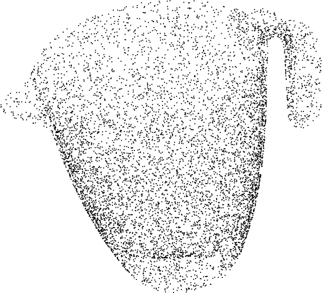
Figure 1: Object set used for grasp learning.

In total, we did 288 simulated runs of our learning method using RobWork. Table I s hows our parameterization of MCMC Kameleon and GDMC for our experiments. The values were learned during a series of preliminary experiments by bringing the acceptance rate close to $\alpha=0.234$ [38].

TABLE I: Parameterization of MCMC Kameleon and GDMC for our experiments.

Iterations+Burn-In	$\gamma$	$n$	$\nu$ [5]	$P_{check}$	$\omega$	$c$
1000+100	1e-05	100	$\frac{2.38}{\sqrt{6}}$	0.5	0.7	$0.0-0.2$

For all experiments we used 5 demonstrated grasps. Modulation values of $c$ for different runs were increments of $0.005$ in the interval $[0.0-0.1]$ and $0.01$ in the interval $[0.1-0.2]$, respectively. As mentioned in Section IV training of $C_{\mathbf{z}}$ was only done during the algorithm’s burn-in to assure convergence.

We further simulated one run for each object using our random walk MH sampler as defined in Section IV to both establish a rough sketch for MCMC Kameleon as well as a base line to compare our proposed learning method to.

At this point we want to clarify that the need for an object model for our experiments only arises, as we evaluate our learning method in simulation. In the event of learning on a real robot, no object model or object geometric information except for its pose is necessary which we assume to be available.

VI Results and Discussion

Table II shows a general overview of the results of our experiments. For each of the objects, the random walk MH sampler yielded, as expected, very poor results. This is evident from the simple design of this sampler. Both the Gaussian and the von-Mises Fisher proposal fail to properly address the high non-linearity and multimodality of our target $\pi(g)$. Further, as of proposing position and orientation independent of each other, the sampler also does not amount for the necessary correlation between them. With the premise that a gripper’s position constrains the reaching movement, synergy among position and orientation is paramount [39].

TABLE II: Successfully sampled grasps of our proposed learning method compared to a random walk MH sampler (Section IV). The values are averaged over varying $c$ (Table I) with the standard deviation denoted in brackets.

	Random Walk	MCMC combined with GDMC
		impartial	weak	strong
Pitcher	0	$143(\raise 1.18056pt\hbox{$\scriptstyle\pm$}48)$	$144(\raise 1.18056pt\hbox{$\scriptstyle\pm$}59)$	$160(\raise 1.18056pt\hbox{$\scriptstyle\pm$}55)$
Pan	2	$216(\raise 1.18056pt\hbox{$\scriptstyle\pm$}46)$	$254(\raise 1.18056pt\hbox{$\scriptstyle\pm$}60)$	$261(\raise 1.18056pt\hbox{$\scriptstyle\pm$}59)$
Plate	1	$180(\raise 1.18056pt\hbox{$\scriptstyle\pm$}46)$	$240(\raise 1.18056pt\hbox{$\scriptstyle\pm$}55)$	$248(\raise 1.18056pt\hbox{$\scriptstyle\pm$}62)$

In contrast, the results of our proposed learning method from Table II clearly indicate that our approach is feasible. No matter how we biased MCMC Kameleon, our learning method, with a few exceptions, consistently found a substantial number of grasps in the hundreds. This capitalizes on MCMC Kameleon’s adaptability to its target which allows it to learn a covariance operator $C_{\mathbf{z}}$ that describes the relation between positions and orientations of grasps for an object. Overfitting of $C_{\mathbf{z}}$ in terms of becoming too local around a specific mode is thwarted by random mode hops. Our conclusions are further strengthened by Figure 2.

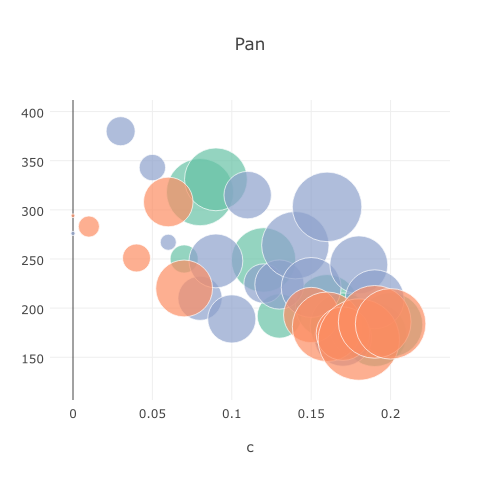
Figure 2: Dispersion plots for all runs w.r.t. $c$ relative to the number of successfully sampled grasps. The cirlces’ sizes denote the surface area of the convex hull of the set of successfully sampled grasps, thence describing the exploratory behavior of the sampler for a given value of $c$. Orange denotes runs with impartial, blue with weak, and green with strong bias. Due to space restrictions values for $c$ were modulated with increments of $0.01$. Best viewed in color.

What is also visible from Figure 2 is the role of $c$. From a geometrical point of view, the value of $c$ used in our kernel essentially constrains the gradient step size in the translational dimensions. Thus, if set to $0$, the gradient ignores the translation completely and only optimizes over the gripper’s orientations. However, by gradually increasing $c$ we allow the sampler to not only explore different orientations of the gripper but also, at the same time, to move along the object to find new grasping points in previously unexplored regions of an object. Clearly, $c$ has to be kept at a reasonable value. Setting it too high results in that the sampler overshoots the object by moving away from it, as of too distant moves in the translational dimensions. From Figure 2 it is evident that for all three objects ideal values for $c$ lie in the range $0.25$ to $0.1$, where in case of the pan this may be extended to $0.15$ as of its elongated shape. Values of $c$ higher than these upper bounds, though yielding better exploration, generally result in less successfully sampled grasps.

Figure 2 also answers our initial question from Section V. If using an impartial bias our learning method performed poorest. Yet, the difference between using either a weak or a strong bias is not substantial anymore. Obviously, a strong bias results in an overfitted covariance operator $C_{\mathbf{z}}$. This again underpins our assumption that grasp learning using only very little object knowledge by its pose and a handful of demonstrated grasps is feasible.

Finally, Figure 3 shows for each object from Figure 1 a few successfully sampled grasps with their corresponding (partial) grasp affordance densities.

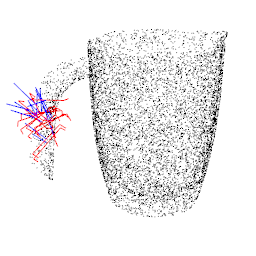
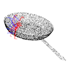
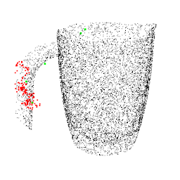
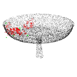
Figure 3: Successfully sampled grasps with corresponding grasp affordance densities. Green dots denote the demonstrated grasps, red dots sampled grasps. For each plot, the value of $c$ is $0.08$ with weak bias. Best viewed in color.

VII Conclusions

We have presented a novel method for active learning of grasps for characterizing an object’s grasp affordance density. We have shown that grasp learning is feasible without any object knowledge except for its pose. Our learning method essentially requires nothing more than a few demonstrated grasps.

Our approach is grounded on MCMC sampling, more specifically a combination of MCMC Kameleon and GDMC. These algorithms each have advantageous characteristics. MCMC Kameleon allows sampling from highly non-linear distributions, whereas GDMC tackles the issue of properly exploring a multimodal distribution. We found that a combination of both ideally fits the problem of model-free, active learning of grasps. Our discussion of experimental results clearly corroborate our conclusions.

We believe that the results of our work are important in that they show that grasp learning essentially can be done blindly. That is, by avoiding to rely on any object geometric knowledge an object’s grasp affordance denisty can still be successfully characterized. This eventually results in more robust and versatile robots.

References

- [1] J. Bohg, A. Morales, T. Asfour, and D. Kragic, “Data-driven Grasp Synthesis — A Survey,” Robotics, IEEE Transactions on, vol. 30, no. 2, pp. 289–309, 2014.
- [2] A. Sahbani, S. El-Khoury, and P. Bidaud, “An Overview of 3D Object Grasp Synthesis Algorithms,” Robotics and Autonomous Systems, vol. 60, no. 3, pp. 326–336, 2012.
- [3] R. Balasubramanian, L. Xu, P. D. Brook, J. R. Smith, and Y. Matsuoka, “Physical Human Interactive Guidance: Identifying Grasping Principles from Human-planned Grasps,” IEEE Transactions on Robotics, vol. 28, no. 4, pp. 899–910, 2012.
- [4] W. K. Hastings, “Monte Carlo Sampling Methods Using Markov Chains and Their Applications,” Biometrika, vol. 57, no. 1, pp. 97–109, 1970.
- [5] D. Sejdinovic, H. Strathmann, M. L. Garcia, C. Andrieu, and A. Gretton, “Kernel Adaptive Metropolis-Hastings,” in Proceedings of the 31st International Conference on Machine Learning, E. P. Xing and T. Jebara, Eds., vol. 32, 2014, pp. 1665–1673.
- [6] C. Sminchisescu and M. Welling, “Generalized darting Monte Carlo,” Pattern Recognition, vol. 44, no. 10–11, pp. 2738–2748, 2011.
- [7] S. Ekvall and D. Kragić, “Interactive Grasp Learning Based on Human Demonstration,” in IEEE International Conference on Robotics and Automation, ICRA’04, vol. 4. IEEE, 2004, pp. 3519–3524.
- [8] ——, “Grasp Recognition for Programming by Demonstration,” in IEEE International Conference on Robotics and Automation, ICRA’05. IEEE, 2005, pp. 748–753.
- [9] H. Kjellström, J. Romero, and D. Kragić, “Visual Recognition of Grasps for Human-to-Robot Mapping,” in IEEE/RSJ International Conference on Intelligent Robots and Systems, IROS’08. IEEE, 2008, pp. 3192–3199.
- [10] J. Romero, H. Kjellström, and D. Kragić, “Human-to-Robot Mapping of Grasps,” in IEEE/RSJ International Conference on Intelligent Robots and Systems, Workshop on Grasp and Task Learning by Imitation, IROS’08, 2008.
- [11] ——, “Modeling and Evaluation of Human-to-Robot Mapping of Grasps,” in International Conference on Advanced Robotics, ICAR’09. IEEE, 2009, pp. 1–6.
- [12] J. Aleotti and S. Caselli, “Grasp Recognition in Virtual Reality for Robot Pregrasp Planning by Demonstration,” in IEEE International Conference on Robotics and Automation, ICRA’06. IEEE, 2006, pp. 2801–2806.
- [13] ——, “Robot Grasp Synthesis from Virtual Demonstration and Topology-preserving Environment Reconstruction,” in IEEE/RSJ International Conference on Intelligent Robots and Systems, IROS’07. IEEE, 2007, pp. 2692–2697.
- [14] Y. Lin and Y. Sun, “Robot Grasp Planning Based on Demonstrated Grasp Strategies,” The International Journal of Robotics Research, pp. 26–42, 2014.
- [15] R. Zöllner, O. Rogalla, R. Dillmann, and J. Zoellner, “Dynamic Grasp Recognition Within the Framework of Programming by Demonstration,” in IEEE International Workshop on Robot and Human Interactive Communication. IEEE, 2001, pp. 418–423.
- [16] Y. Li and N. S. Pollard, “A Shape Matching Algorithm for Synthesizing Humanlike Enveloping Grasps,” in IEEE-RAS International Conference on Humanoid Robots, HUMANOIDS’05. IEEE, 2005, pp. 442–449.
- [17] F. Kyota, T. Watabe, S. Saito, and M. Nakajima, “Detection and Evaluation of Grasping Positions for Autonomous Agents,” in International Conference on Cyberworlds. IEEE, 2005, pp. 460–468.
- [18] A. Herzog, P. Pastor, M. Kalakrishnan, L. Righetti, J. Bohg, T. Asfour, and S. Schaal, “Learning of Grasp Selection Based on Shape-templates,” Autonomous Robots, vol. 36, no. 1-2, pp. 51–65, 2014.
- [19] S. Ekvall and D. Kragić, “Learning and Evaluation of the Approach Vector for Automatic Grasp Generation and Planning,” in IEEE International Conference on Robotics and Automation, ICRA’07. IEEE, 2007, pp. 4715–4720.
- [20] J. Tegin, S. Ekvall, D. Kragic, J. Wikander, and B. Iliev, “Demonstration-based Learning and Control for Automatic Grasping,” Intelligent Service Robotics, vol. 2, no. 1, pp. 23–30, 2009.
- [21] J. Aleotti and S. Caselli, “Part-based Robot Grasp Planning from Human Demonstration,” in IEEE International Conference on Robotics and Automation, ICRA’11. IEEE, 2011, pp. 4554–4560.
- [22] K. Hsiao and T. Lozano-Perez, “Imitation Learning of Whole-body Grasps,” in IEEE/RSJ International Conference on Intelligent Robots and Systems, IROS’06. IEEE, 2006, pp. 5657–5662.
- [23] M. Do, T. Asfour, and R. Dillmann, “Towards a Unifying Grasp Representation for Imitation Learning on Humanoid Robots,” in IEEE International Conference on Robotics and Automation, ICRA’11. IEEE, 2011, pp. 482–488.
- [24] O. Kroemer, R. Detry, J. Piater, and J. Peters, “Combining Active Learning and Reactive Control for Robot Grasping,” Robotics and Autonomous Systems, vol. 58, no. 9, pp. 1105–1116, 2010.
- [25] P. Pastor, L. Righetti, M. Kalakrishnan, and S. Schaal, “Online Movement Adaptation based on Previous Sensor experiences,” in IEEE/RSJ International Conference on Intelligent Robots and Systems, IROS’11. IEEE, 2011, pp. 365–371.
- [26] E. Oztop and M. A. Arbib, “Schema Design and Implementation of the Grasp-related Mirror Neuron System,” Biological Cybernetics, vol. 87, no. 2, pp. 116–140, 2002.
- [27] M. Hueser, T. Baier, and J. Zhang, “Learning of Demonstrated Grasping Skills by Stereoscopic Tracking of Human Head Configuration,” in IEEE International Conference on Robotics and Automation, ICRA’06. IEEE, 2006, pp. 2795–2800.
- [28] C. de Granville, J. Southerland, and A. H. Fagg, “Learning Grasp Affordances Through Human Demonstration,” in International Conference on Development and Learning, ICDL’06. IEEE, 2006.
- [29] D. R. Faria, R. Martins, J. Lobo, and J. Dias, “Extracting Data from Human Manipulation of Objects Towards Improving Autonomous Robotic Grasping,” Robotics and Autonomous Systems, vol. 60, no. 3, pp. 396–410, 2012.
- [30] R. Detry, D. Kraft, O. Kroemer, L. Bodenhagen, J. Peters, N. Krüger, and J. Piater, “Learning Grasp Affordance Densities,” Paladyn, vol. 2, no. 1, pp. 1–17, 2011.
- [31] J. D. Sweeney and R. Grupen, “A Model of Shared Grasp Affordances From Demonstration,” in IEEE-RAS International Conference on Humanoids Robots, HUMANOIDS’07. IEEE, 2007, pp. 27–35.
- [32] M. Kopicki, R. Detry, F. Schmidt, C. Borst, R. Stolkin, and J. Wyatt, “Learning Dexterous Grasps that Generalise to Novel Objects by Combining Hand and Contact Models,” in IEEE International Conference on Robotics and Automation, ICRA’14., May 2014, pp. 5358–5365.
- [33] M. Kopicki, R. Detry, M. Adjigble, R. Stolkin, A. Leonardis, and J. L. Wyatt, “One-shot Learning and Generation of Dexterous Grasps for Novel Objects,” vol. 35, no. 8, pp. 959–976, 2016.
- [34] A. T. Miller and P. K. Allen, “Examples of 3D Grasp Quality Computations,” in IEEE International Conference on Robotics and Automation, 1999. Proceedings, ICRA’99., vol. 2. IEEE, 1999, pp. 1240–1246.
- [35] P. Zech, H. Xiong, and J. Piater, “Rotation Optimization on the Unit Quaternion Manifold and its Application for Robotic Grasping,” in IMA Conference on Mathematics of Robotics. IMA, 2015, to appear.
- [36] M. Lang, M. Kleinsteuber, O. Dunkley, and S. Hirche, “Gaussian Process Dynamical Models Over Dual Quaternions,” in European Control Conference (ECC), 2015. IEEE, 2015, pp. 2847–2852.
- [37] L.-P. Ellekilde and J. A. Jorgensen, “RobWork: A Flexible Toolbox for Robotics Research and Education,” in 41st International Symposium on Robotics (ISR) and 2010 6th German Conference on Robotics (ROBOTIK). VDE, 2010, pp. 1–7.
- [38] C. Andrieu and J. Thoms, “A Ttutorial on Adaptive MCMC,” Statistics and Computing, vol. 18, no. 4, pp. 343–373, 2008.
- [39] A. Roby-Brami, N. Bennis, M. Mokhtari, and P. Baraduc, “Hand Orientation for Grasping Depends on the Direction of the Reaching Movement,” Brain Research, vol. 869, no. 1–2, pp. 121 – 129, 2000.