Spikes as Regularizers

Abstract

We present a confidence-based single-layer feed-forward learning algorithm Spiral (Spike Regularized Adaptive Learning) relying on an encoding of activation spikes. We adaptively update a weight vector relying on confidence estimates and activation offsets relative to previous activity. We regularize updates proportionally to item-level confidence and weight-specific support, loosely inspired by the observation from neurophysiology that high spike rates are sometimes accompanied by low temporal precision. Our experiments suggest that the new learning algorithm Spiral is more robust and less prone to overfitting than both the averaged perceptron and Arow.

1 Confidence-weighted Learning of Linear Classifiers

The perceptron (Rosenblatt, 1958) is a conceptually simple and widely used discriminative and linear classification algorithm. It was originally motivated by observations of how signals are passed between neurons in the brain. We will return to the perceptron as a model of neural computation, but from a more technical point of view, the main weakness of the perceptron as a linear classifier is that it is prone to overfitting. One particular type of overfitting that is likely to happen in perceptron learning is feature swamping (Sutton et al., 2006), i.e., that very frequent features may prevent co-variant features from being updated, leading to catastrophic performance if the frequent features are absent or less frequent at test time. In other words, in the perceptron, as well as in passive-aggressive learning Crammer et al. (2006), parameters are only updated when features occur, and rare features therefore often receive inaccurate values.

There are several ways to approach such overfitting, e.g., capping the model’s supremum norm, but here we focus on a specific line of research: confidence-weighted learning of linear classifiers. Confidence-weighted learning explicitly estimates confidence during induction, often by maintaining Gaussian distributions over parameter vectors. In other words, each model parameter is interpreted as a mean, and augmented with a covariance estimate. Confidence-Weighted Learning CWL (Dredze et al., 2008) was the first learning algorithm to do this, but Crammer et al. (2009) later introduced Adaptive Regularization of Weight Vectors (Arow), which is a simpler and more effective alternative:

Arow passes over the data, item by item, computing a margin, i.e., a dot product of a weight vector $\mathbf{\mu}$ and the item, and updating $\mathbf{\mu}$ and a covariance matrix $\Sigma$ in a standard additive fashion. As in CWL, the weights – which are interpreted as means – and the covariance matrix form a Gaussian distribution over the weight vectors. Specifically, the confidence is $\mathbf{x}^{\top}\Sigma\mathbf{x}$. We add a smoothing constant $r(=0.1)$ and compute the learning rate $\alpha$ adaptively:

$$\alpha=\frac{\max(0,1-y\mathbf{x}^{\top}\mathbf{\mu})}{\mathbf{x}^{\top}\Sigma\mathbf{x}+r}$$ (1)

We then update $\mathbf{\mu}$ proportionally to $\alpha$, and update the covariance matrix as follows:

$$\Sigma\leftarrow\frac{\Sigma-\Sigma\mathbf{x}\mathbf{x}^{\top}\Sigma}{\mathbf{x}^{\top}\Sigma\mathbf{x}+r}$$ (2)

CWL and Arow have been shown to be more robust than the (averaged) perceptron in several studies (Crammer et al., 2012; Søgaard and Johannsen, 2012), but below we show that replacing binary activations with samples from spikes can lead to better regularized and more robust models.

2 Spikes as Regularizers

2.1 Neurophysiological motivation

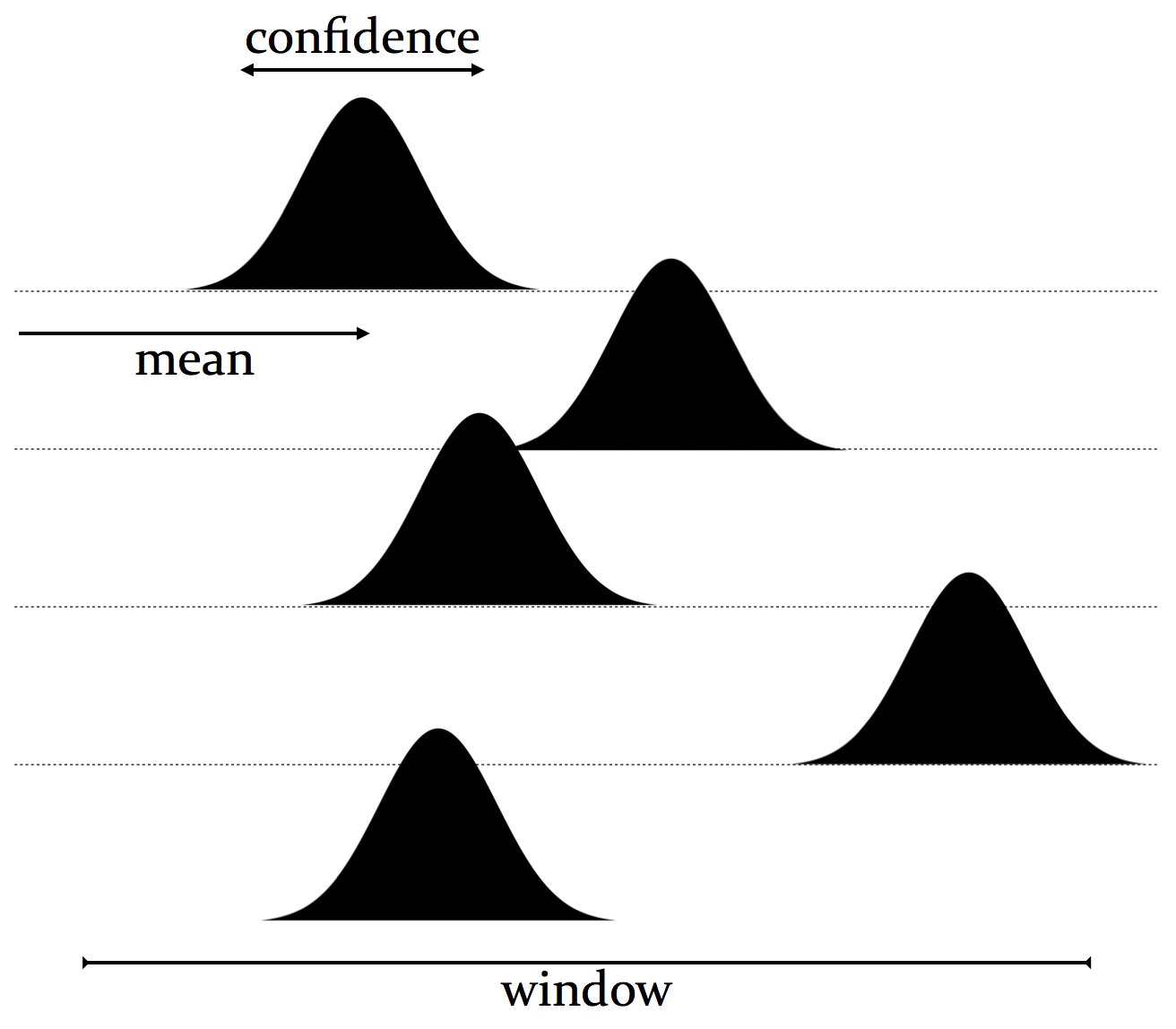
Neurons do not fire synchronously at a constant rate. Neural signals are spike-shaped with an onset, an increase in signal, followed by a spike and a decrease in signal, and with an inhibition of the neuron before returning to its equilibrium. Below we simplify the picture a bit by assuming that spikes are bell-shaped (Gaussians).

The learning algorithm (Spiral) which we will propose below, is motivated by the observation that spike rate (the speed at which a neuron fires) increases the more a neuron fires (Kawai and Sterling, 2002; Keller and Takahashi, 2015). Futhermore, Keller and Takahashi (2015) show that increased activity may lead to spiking at higher rates with lower temporal precision. This means that the more active neurons are less successful in passing on signals, leading the neuron to return to a more stable firing rate. In other words, the brain performs implicit regularization by exhibiting low temporal precision at high spike rates. This prevents highly active neurons from swamping other co-variant, but less active neurons. We hypothesise that implementing a similar mechanism in our learning algorithms will prevent feature swamping in a similar fashion.

Finally, Blanco et al. (2015) show that periods of increased spike rate lead to a smaller standard deviation in the synaptic weights. This loosely inspired us to implement the temporal imprecision at high spike rates by decreasing the weight’s standard deviation.

2.2 The algorithm

In a single layer feedforward model, such as the perceptron, sampling from Gaussian spikes only effect the input, and we can therefore implement our regularizer as noise injection (Bishop, 1995). The variance is the relative confidence of the model on the input item (same for all parameters), and the means are the parameter values. We multiply the input by the inverse of the sample, reflecting the intuition that highly active neurons are less precise and more likely to drop out, before we clip the sample from 0 to 1.

We give the pseudocode in Algorithm 1, following the conventions in Crammer et al. (2009).

1:  $r=0.1,\mathbf{\mu}_{0}=\mathbf{0},\Sigma_{0}=I,\{\mathbf{x}_{t}\mid\mathbf{x}_{t}\in\mathbb{R}^{d}\},v=0$

2:  for $t<T$ do

3:     $\mathbf{x}_{t}=\mathbf{x}_{t}\cdot$

4:     if $v_{t}>v$ then

5:        $v=v_{t}$

6:     end if

7:     $v_{t}=\mathbf{x}_{t}^{\top}\Sigma_{t-1}\mathbf{x}_{t}$ (sampling activations from Gaussian spikes)

8:     $v_{t}=0<v_{t}<1$ (clipping values outside the [0,1] window)

9:     $\mathbf{\nu}_{t}\sim\mathcal{N}(\mathbf{\mu}_{t-1},\frac{v_{t}}{v})$

10:     $\mathbf{x}_{t}=\mathbf{x}_{t}\cdot(1-\mathbf{\nu}_{t})$

11:     $m_{t}=\mathbf{\mu}_{t-1}\cdot\mathbf{x}_{t}$

12:     if $m_{t}y_{t}<1$ then

13:        $\alpha_{t}=\frac{\max(0,1-y_{t}\mathbf{x}_{t}^{\top}\mathbf{\mu}_{t-1})}{\mathbf{x}_{t}^{\top}\Sigma_{t-1}\mathbf{x}_{t}+r}$

14:        $\mathbf{\mu}_{t}=\mathbf{\mu}_{t-1}+\alpha_{t}\Sigma_{t-1}y_{t}\mathbf{x}_{t}$

15:        $\Sigma_{t}=\frac{\Sigma_{t-1}-\Sigma_{t-1}\mathbf{x}_{t}\mathbf{x}_{t}^{\top}\Sigma_{t-1}}{\mathbf{x}_{t}^{\top}\Sigma\mathbf{x}_{t}+r}$

16:     end if

17:  end for

18:  return  $\mathbf{\mu}_{T},\Sigma_{T}$

Algorithm 1 Spiral. Except for lines 8–10, this is identical to Arow.

Figure 1: Sampling activations from Gaussian spikes.

3 Experiments

3.1 Main experiments

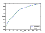
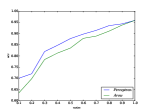
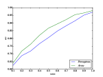
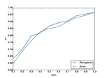
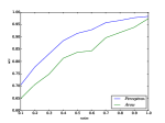
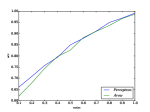
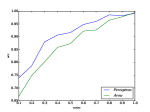
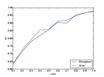
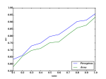
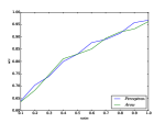
We extract 10 binary classification problems from MNIST, training on odd data points, testing on even ones. Since our algorithm is parameter-free, we did not do explicit parameter tuning, but during the implementation of Spiral, we only experiment with the first of these ten problems (left, upper corner). To test the robustness of Spiral relatively to the perceptron and Arow, we randomly corrupt the input at test time by removing features. Our set-up is inspired by Globerson and Roweis (2006). In the plots in Figure 2, the $x$-axis presents the number of features kept (not deleted).

Arow

Spiral

Figure 2: Performance over noise levels (percentage of features kept). First two lines compare the perceptron (blue) and Arow (green); the third and fourth compare the perceptron (blue) and Spiral (green).

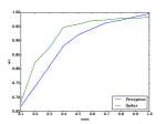
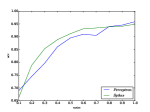
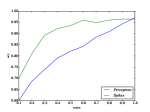
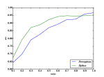
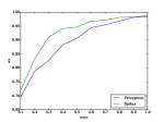
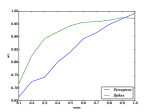
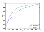
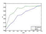
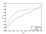
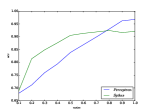
We observe two tendencies in the results: (i) Spiral outperforms the perceptron consistently with up to 80% of the features, and sometimes by a very large margin; except that in 2/10 cases, the perceptron is better with only 10% of the features. (ii) In contrast, Arow is less stable, and only improves significantly over the perceptron under mid-range noise levels in a few cases. The perceptron is almost always superior on the full set of features, since this is a relatively simple learning problem, where overfitting is unlikely, unless noise is injected at test time.

3.2 Practical Rademacher complexity

We compute Spiral’s practical Rademacher complexity as the ability of Spiral to fit random re-labelings of data. We randomly label the above dataset ten times and compute the average error reduction over a random baseline. The perceptron achieves a 5% error reduction over a random baseline, on average, overfitting quite a bit to the random labelling of the data. In contrast, Spiral only reduces 0.6% of the errors of a random baseline on average, suggesting that it is almost resilient to overfitting on this dataset.

4 Conclusion

We have presented a simple, confidence-based single layer feed-forward learning algorithm Spiral that uses sampling from Gaussian spikes as a regularizer, loosely inspired by recent findings in neurophysiology. Spiral outperforms the perceptron and Arow by a large margin, when noise is injected at test time, and has lower Rademacher complexity than both of these algorithms.

Acknowledgments

References

- Bishop [1995] Cristopher Bishop. Training with noise is equivalent to tikhonov regularization. Neural Computation, 7(1):108–116, 1995.
- Blanco et al. [2015] Wilfredo Blanco, Catia Pereira, Vinicius Cota, Annie Souza, Cesar Renno-Costa, Sharlene Santos, Gabriella Dias, Ana Guerreiro, Adriano Tort, Adriao Neto, and Sidarta Ribeiro. Synaptic homeostasis and restructuring across the sleep-wake cycle. PLoS Computational Biology, 11:1–29, 2015.
- Crammer et al. [2006] Koby Crammer, Ofer Dekel, Joseph Keshet, Shai Shalev-Shwartz, and Yoram Singer. Online passive-agressive algorithms. Journal of Machine Learning Research, 7:551–585, 2006.
- Crammer et al. [2009] Koby Crammer, A Kulesza, and Mark Dredze. Adaptive regularization of weighted vectors. In NIPS, 2009.
- Crammer et al. [2012] Koby Crammer, Mark Dredze, and Fernando Pereira. Confidence-weighted linear classification for text categorization. Journal of Machine Learning Research, 13:1891–1926, 2012.
- Dredze et al. [2008] Mark Dredze, Koby Crammer, and Fernando Pereira. Confidence-weighted linear classification. In ICML, 2008.
- Globerson and Roweis [2006] Amir Globerson and Sam Roweis. Nightmare at test time: robust learning by feature deletion. In ICML, 2006.
- Kawai and Sterling [2002] Fusao Kawai and Peter Sterling. cgmp modulates spike responses of retinal ganglion cells via a cgmp-gated current. Visual Neuroscience, 19:373–380, 2002.
- Keller and Takahashi [2015] Clifford Keller and Terry Takahashi. Spike timing precision changes with spike rate adaptation in the owl’s auditory space map. Journal of Neurophysiology, 114:2204–2219, 2015.
- Rosenblatt [1958] Frank Rosenblatt. The perceptron: a probabilistic model for information storage and organization in the brain. Psychological Review, 65(6):386–408, 1958.
- Søgaard and Johannsen [2012] Anders Søgaard and Anders Johannsen. Robust learning in random subspaces: equipping NLP against OOV effects. In COLING, 2012.
- Sutton et al. [2006] Charles Sutton, Michael Sindelar, and Andrew McCallum. Reducing weight undertraining in structured discriminative learning. In NAACL, 2006.