A new method to reduce the statistical and systematic uncertainty of chance coincidence backgrounds measured with waveform digitizers

Abstract

A new method for measuring chance-coincidence backgrounds during the collection of coincidence data is presented. The method relies on acquiring data with near-zero dead time, which is now realistic due to the increasing deployment of flash electronic-digitizer (waveform digitizer) techniques. An experiment designed to use this new method is capable of acquiring more coincidence data, and a much reduced statistical fluctuation of the measured background. A statistical analysis is presented, and used to derive a figure of merit for the new method. Factors of four improvement over other analyses are realistic. The technique is illustrated with preliminary data taken as part of a program to make new measurements of the prompt fission neutron spectra at Los Alamos Neutron Science Center. It is expected that the these measurements will occur in a regime where the maximum figure of merit will be exploited.

1 Introduction and Motivation

The impact of backgrounds on the statistical significance of an experiment is of such importance that Knoll discusses it in his seminal book, Radiation Detection and Measurement, just as soon as sufficient statistical background is presented to understand the subject[1]. One of the compromises in performing an experiment is to reduce the amount of time spent taking foreground data (and losing counts and statistics), to take background data. If too much time is spent on the background measurement, then valuable foreground statistics are lost. On the other hand, if insufficient background data are obtained, the quality of the foreground data is compromised by a poor background subtraction. In the book, Knoll presents an expression for the optimal division of time between the two stages of data collection. The question of systematic changes between the two separate measurements is not considered — but is often apparent, for example if a background normalization factor has to be applied during the data analysis. The complications introduced by backgrounds warrant all reasonable attempts to remove the background.

Over the years the coincidence technique has proven to be a powerful method to reduce or even remove large backgrounds. Knoll also discusses the nature of chance coincidences as a source of background in coincidence experiments, and presents a simple formula to estimate the chance coincident rate. The formula is traditionally used to help design layouts for experiments, and provide estimates for the quality of the data when setting up an experiment. The formula for the rate of chance coincidences, $r_{\gamma}$, between two detectors, counting at rates $r_{a}$ and $r_{b}$, during a coincidence time window with width, $\Delta_{t}$, is

$$r_{\gamma}=r_{a}r_{b}\Delta_{t}.$$ (1)

A key concept in the derivation of Eq. (1) is the dead time, $t_{d}$, of the detector, electronics and the data acquisition system (DAQ), even though $t_{d}$ is not explicit in the formula. Eq. (1) is only valid if $r_{a}t_{d}\ll 1$ and $r_{b}t_{d}\ll 1$.

While Eq. (1) is well known, we are not aware of any analyses using it to measure the detailed background shape in a coincidence measurement, presumably due to the difficulty in measuring $r_{a}$ and $r_{b}$ reliably. High singles rates impose challenges in acquiring, saving and analyzing complete data sets using an event-triggered DAQ with very real dead-time concerns.

The current work is motivated by the increasing use of flash digitizers running semi-continuously (waveform digitizers), with waveform analysis capabilities on board, to build high throughput DAQs with no contribution to dead time (see e.g. [2, 3, 4]). When combined with computers with large storage areas it is now realistic to record complete data sets of all the signals from all the detectors with dead time due only to signal overlap (pileup) in the detector and preamps. Coincidences are identified, in software, later in the analysis.

With such a DAQ we show that Knoll’s expression to estimate chance coincidence rates can now be used to determine a bin-by-bin measurement of the background obtained simultaneously with the foreground. In addition to reducing systematic uncertainties, this allows to obtain the maximal signal statistics, and it will be shown yields a very small statistical uncertainty on the background measurement. The question of how much time to spend on the foreground and background measurements becomes trivial — do both all the time!

Before proceeding, we rewrite Eq. (1) in terms of the counts observed in an experiment, which also allows us to easily quantify the statistical uncertainty. The numbers of counts, $a$ and $b$, obtained in each detector, and summed over $N$ measurements, are then related to the measured singles rates by $a=r_{a}N\Delta_{t}$ and $b=r_{b}N\Delta_{t}$, and the number of chance coincidences, $\gamma$, in the time-difference window, $\Delta_{t}$, is then

$$\gamma\pm\sigma_{\gamma}={\frac{ab}{N}}\pm\sqrt{\frac{ab(a+b)}{N^{2}}},$$ (2)

where $\sigma_{\gamma}$ is the statistical uncertainty on $\gamma$, assuming Gaussian statistics for $a$ and $b$.

In the next two sections we briefly describe an experiment being developed to measure the prompt fission neutron spectrum (PFNS) on ²³⁹Pu[5], and then in more detail, two possible analysis procedures which use Eq. (2) to estimate backgrounds for this experiment. In the following section we contrast this approach with more traditional methods for measuring backgrounds — resulting in the derivation of a figure of merit for the new method of analysis. There then follows a comment on the data-acquisition requirements to obtain a data set which is complete enough to apply the current technique (and a numerical validation of $r_{a}t_{d}\ll 1$ and $r_{b}t_{d}\ll 1$ for the example experiment). Further formulas derived from Eq. (2), and which are needed to implement a full analysis, are presented in a short series of appendices.

2 Example Experiment With Complicated Backgrounds

Data for outgoing fission neutrons from neutron induced fission of ²³⁹Pu are used to illustrate the techniques discussed here. The coincidence nature of the experiment arises from detecting one of the fission fragments together with a neutron generated in the fission process. The detection of a fission fragment implicates the timing properties of the incoming neutron.

Figure 1: Conceptual layout for a two-arm time of flight ²³⁹Pu$(n;f,xn)$ experiment, detecting fission fragments in a parallel-plate avalanche counter(PPAC), (which implicates the timing of an incoming neutron, with respect to the neutron production time signal from the t₀ pick off), and fission neutrons are detected in the lithium glass neutron detectors.

Figure 2: Structure of the proton beam to WNR.

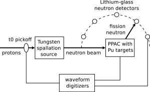
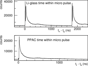
The data were acquired as part of the development for the PFNS measurements currently being performed at the WNR/LANSCE neutron spallation source[6]. A conceptual figure of the experiment is shown in fig. 1. Beam delivery was structured on two time scales (fig. 2): micro pulses of protons (each making their own timing signal, $t_{0}$, and forming their source of spallation neutrons) occur at nominal 1.8$\mu$s intervals; and macro pulses, being groups of 347 micro pulses, separated by several milliseconds. Only two of every three macro pulses were delivered to WNR.

Model ZT4441-DP-PXI digitizers[7] (sample rate 400Ms^-1) were used to acquire 1ms long waveforms spanning the duration of complete macro pulses. Triggers for most of the digitizers were distributed across a PXI bus from a self-triggering digitizer receiving the $t_{0}$ signal. ZT1000PXI cards[7] enabled distribution of the trigger and a stable reference clock between PXI crates. Up to 22 lithium-glass detectors and digitizer channels were used to detect the outgoing neutrons[8]. A further ten digitizer channels processed the signals from a multi-segment parallel-plate avalanche counter (PPAC) for detecting fission fragments[9]. Each waveform was analyzed on board the digitizer using custom firmware, to generate a list of parameters such as a time stamp, the baseline height, and two integrals of the peak area at different time offsets from the peak position, for all the peaks found in the waveform. The lists of parameters were read from each digitizer across the PXI bus into computer memory for storage and further processing, before preparing the digitizers to process another macro pulse.

The times within a macro pulse of individual peaks in the $t_{0}$, PPAC and lithium-glass signals are denoted as $t_{0}$, $t\!_{f}$, and $t_{n}$, respectively; and the lists of these times as reported by the digitizers are denoted by $\{t_{0}\}$, $\{t\!_{f}\}$, and $\{t_{n}\}$, respectively.

Figure 3: Distribution of singles events within the macro pulses for one lithium-glass detector and one PPAC foil. Cuts to reduce backgrounds have been applied (see text).

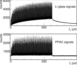
Backgrounds from several sources are present in the data. Some of the more significant sources are: (1) fast neutrons generated from interactions other than fission from a particular sample foil; (2) a ”sea” of thermal and epithermal neutrons (see the rising and decaying baseline in the top panel of fig. 3); (3) sensitivity of the neutron detectors to gamma rays; and (4) a small residual sensitivity of the PPAC to the large alpha decay rate of the plutonium samples (fig. 3, lower panel).

These backgrounds remain significant, even after applying some simple background reduction cuts, such as a cuts to separate neutrons from gamma rays in the lithium-glass detectors (exploiting the +4.78 MeV Q-value of the ⁶Li($n,t)\alpha$ reaction), and also PPAC pulse-height cuts to optimize fission–alpha-decay separation. We anticipate using a more complete set of cuts for a final analysis of the data from these experiments, but we still expect many components of the background to remain.

3 Coincidence Analysis

Given the lists of time stamps, $\{t_{0}\}$, $\{t\!_{f}\}$, $\{t_{n}\}$ for the singles data from each detector, two methods of coincidence analysis are presented to fully identify the triplet of times $\{t_{0},t\!_{f}\!,t_{n}\}$, of a fission event. Both methods identify two lists of time doublets (or coincidences). The triplet of a fission event is then a double coincidence, formed with one coincidence from each list, matched on the same time of their common signal. The two methods are distinguished by whether the coincidence pair $\{t\!_{f},t_{n}\}$ is one of the initial lists of coincidences (method one), or implied later (method two), and which signal is used as the common signal between the lists ($t\!_{f}$ in method one, and $t_{0}$ in method two). Details of each method are given below. While method one follows the natural time ordering of detected signals for a fission event, the discussion below shows that method two leads to a more detailed understanding of the backgrounds due to chance coincidences.

Figure 4: Lithium glass detector (upper panel), and PPAC (lower panel) signal times within the micro-pulse structure.

Figure 5: Time of flight histogram (upper curve, black online) for coincidences from one lithium glass–PPAC combination, correlated on a common $t_{0}$, and the measured background from chance coincidences (lower curve, red online).

In the first method, the lists of $\{t\!_{f}\}$ and $\{t_{n}\}$, from which fig. 3 was made, are searched to form a list of coincidences $\{t\!_{f}\!,t_{n}\}$. At this point a histogram of $t_{n}\!-t\!_{f}$ could be filled, and a measurement of the background due to chance coincidences could be derived using Eq. (2). The quantities $a$ and $b$ would be taken from the singles histograms of fig. 3, and $N$ would be the number of macro pulses used to acquire the data.

To complete the first method, pairs of $\{t_{0},t\!_{f}\}$ are also identified, and then correlated with the $\{t\!_{f}\!,t_{n}\}$ pairs on a common $t\!_{f}\!$. Note that in this method, the background due to chance-coincidences is determined before the fission event time is correlated with the neutron production time. This makes it difficult to use the first method to study the background dependence on $t\!_{f}-t_{0}$. Therefore a second method was found, which although leading less directly to the $\{t\!_{f},f_{n}\}$ coincidences, allows to measure the background even with complicated cuts.

Figure 6: Time of flight histogram (upper curves, black online) for coincidences between many combinations of lithium glass–PPAC detectors correlated on a common $t_{0}$, and the measured background due to chance coincidences (lower curves, red online), for four different ranges of $t\!_{f}-t_{0}$, and summed over all available lithium-glass–PPAC combinations.

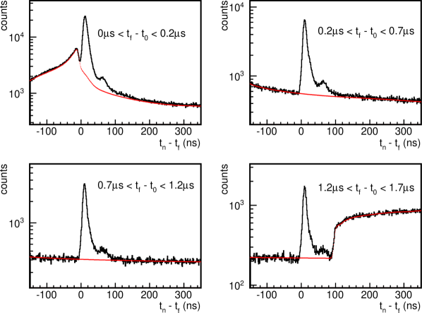
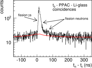
For the second method, lists of $\{t_{0},t\!_{f}\}$ between the fission-fragment and $t_{0}$ signals (the same list as used in the final stages of the first method), and between the neutron detector and $t_{0}$ signals $\{t_{0},t_{n}\}$ are formed, and appropriate histograms filled (fig. 4). The $t_{0}$ times are not generated by a Poisson process and so Eq. (2) is not yet applicable. A second search is then used to correlate pairs of $\{t_{0},t\!_{f}\}$ and $\{t_{0},t_{n}\}$ on a common $t_{0}$, thus allowing to fill the $t_{n}\!-t\!_{f}$ histogram (fig. 5). $\{t_{0},t\!_{f}\}$ and $\{t_{0},t_{n}\}$ are each driven by a (time-dependent) Poisson process, and so Eq. (2) can be used to determine a background due to chance coincidences for the histogram of $t_{n}\!-t\!_{f}$ for a common $t_{0}$ (red curve on fig 5). The $a$ and $b$ values are taken from the histograms of fig. 4, and $N$ is now the total number of $t_{0}$ signals. In contrast to the first method, the background can still be determined even with cuts applied to the fission time, $t\!_{f}-t_{0}$, by applying cuts to the list of $\{t_{0},t\!_{f}\}$ before performing the second stage of searching, and then filling the histograms of figs. 4 and 5. Fig. 6 shows such an analysis.

For the analyses both with and without cuts (figs. 5 and 6), attention is brought to the smaller peak in the double coincidence data for $50{\rm ns}<t_{n}\!-t\!_{f}<100{\rm ns}$, the tails of which are of interest (especially the slower times, i.e. $<240$ keV outgoing neutron energy)[5]. The large background under the low energy tail (larger $t_{n}\!-t\!_{f}$) makes this region especially suitable for the new background measurement techniques (see the figure-of-merit discussion below). The larger peak ($0{\rm ns}<t_{n}\!-t\!_{f}<50{\rm ns}$) is dominated by fission photons, which are to be removed by cuts in a more complete analysis, but should also contain events from fission with higher energy outgoing neutrons. Features of the background shapes are better understood once the full two-dimensional background is presented below, but it is important to note from fig. 6, firstly that the backgrounds are not flat and secondly that the background shape varies with the incident neutron energy.

As a practical matter, data processing for the background analysis may be performed either before or after adding independent subsets of the data set, depending on whether significant systematic changes in the count rates have occurred or not. Systematic changes between subsets require independent background analyses, whereas summing over independent subsets requires less resources (e.g. CPU time and memory) to process the data. Both approaches work (see A), or even a combination, depending on the details of the experiment. The current data were acquired in four hour subsets spanning about one hundred hours and one background analysis was performed on the summed results.

Figure 7: Measured two-dimensional correlations (white indicates zero counts) between $\{t\!_{f}-t_{0}\}$ and $\{t_{n}\!-t_{0}\}$ (left), and the measured background quantity $\gamma(t_{a},t_{b})$ (right). Overlaid diagonal lines (red online) mark the limits used to project one dimensional distributions of fig. 5 (and 6).

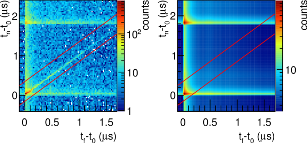
A second practical consideration is how to handle the two-dimensional (2D) nature of Eq. (2). The values of $a$ and $b$ each depend on one or the other of the two times for the random processes, in this case, $t\!_{f}-t_{0}$ and $t_{n}\!-t_{0}$, so that $\gamma(t_{a},t_{b})$ is a dyadic function of these times. The one-dimensional (1D) background presented in fig. 5 is a projection along lines parallel to the primary diagonal of $\gamma(t_{a},t_{b})$ (see right hand side of fig. 7), just as the coincidence spectrum itself is a projection along the same lines of a correlation plot between $\{t\!_{f}-t_{0}\}$ and $\{t_{n}\!-t_{0}\}$ (left hand side of fig. 7). Processing the complete 2D background space is not always necessary. Firstly, it is only necessary to process that section of the space near the coincidence diagonal (between the red lines in fig. 7). Secondly, for most analyses a direct determination of the 1D distribution can proceed using the formulas of B. If a 2D analysis is still required (e.g. the next four paragraphs), a lower resolution will often suffice.

Understanding the 2D nature of the problem can provide insights into the results obtained, as features of the 1D background shape can be attributed to summing over different features in the 2D plot of fig. 7. These features will become more or less dominant depending on the summation regions used due to cuts (such as those on $t\!_{f}-t_{0}$ in fig. 6), and also due to the sensitivity of each detector to the physical processes contributing to the background.

For example, one feature of the 1D background in fig. 5 is a modestly peaked structure at small time differences. The 2D distribution shows that the small 1D peak arises from a very high and narrow peak, located at the intersection of the high count rate bands near $t\!_{f}-t_{0}\approx 0$, and $t_{n}\!-t_{0}\approx 0$, with tails following along each of the band. The peak is then a result of chance coincidences between fission neutrons (or other beam induced neutrons) and fission signals. The upper left panel of fig. 6 shows a much stronger peak, now shifted to slightly negative $t_{n}\!-t\!_{f}$. In this case, the two most forward angle neutron detectors (not included in fig. 7) are very sensitive to direct scattering of neutrons from the beam and would show up in the two-dimensional analysis as a strong enhancement of the horizontal band near $t_{n}\!-t_{0}\approx 0\mu{\rm s}$, and the 1D peak arises from chance coincidences between the scattered beam neutrons and fissions[10]. Similarly, the step in the background in the lower right panel of fig. 6 arises from the scattering into these two detectors, now from beam neutrons from the next micro pulse at $t_{n}\!-t_{0}\approx 1.8\mu{\rm s}$.

On the other hand, the low background in the center of the 2D distribution sums over many channels in the 1D projection, and can therefore become comparable in magnitude to the peak at $t_{n}\!-t_{0}\approx t\!_{f}-t_{0}\approx 0$. The instantaneous neutron beam intensity is reduced in this region. Therefore chance coincidences in this region are more likely to involve neutrons from the ”sea” of thermal and epithermal neutrons, and/or the plutonium alpha decays events in the PPAC.

Another striking aspect of the background measurement in figs. 5 and 6 is how small the statistical fluctuations on the background measurements are. In fact, the one-sigma uncertainty bars are marked on the figure, and even on the log plot are hard to see. The origin of the small uncertainties derives from both the large number of counts available in the two input spectra, and also from dividing by a large value of $N$ (in this case $N\approx 2.5\times 10^{9}$). A full statistical analysis, including a derivation of the covariance matrix between elements of the background measurement is presented in C.

The method is extensible to more complicated analysis, such as calculating the background as a function of a singles parameter against the time difference of the coincidences; or even then summing over the time difference coordinate. For example, full analysis of the example experiment will apply a kinematic cut in the outgoing time-of-flight versus outgoing neutron pulse height space to remove the photon peak from figs. 5 and 6, requiring summing the background contribution only in the same region. Other possibilities, perhaps more suitable for other experiments, include projecting the background onto the axis of the singles parameter (or combination of singles parameters); or to extend Eq. 2 to higher multiplicity coincidences.

4 Figure of Merit

We now consider the impact of these results when deciding how much time to spend acquiring data, by contrasting the signal-to-noise ratio of traditional methods with that for the new method.

With a system that does not record all the singles data, it is often necessary to dedicate some fraction, $\tau$, of the time to measuring the foreground (with background), and the remaining fraction ($1-\tau$) to measuring the background alone. If the strength of the background relative to the foreground is $\phi$, then the number of counts, $c_{f+b}$ and $c_{b}$ obtained during the two parts of the measurement are

$$c_{f+b} =C(1+\phi)\tau\pm\sqrt{C(1+\phi)\tau},$$ (3)

$$c_{b} =C\phi(1-\tau)\pm\sqrt{C\phi(1-\tau)},$$ (4)

where $C$ is a characteristic constant of the experiment (representing the number of foreground counts if no time is dedicated to the background measurement, i.e. $\tau=1$, any $\phi$). The number of foreground counts, $c_{f}$, is obtained from these equations by normalizing $c_{b}$ and subtracting from $c_{f+b}$:

$$\begin{split}c_{f}&=c_{f+b}-\frac{\tau}{1-\tau}c_{b}\\ &=C\tau\pm\sqrt{\frac{C\tau(1+\phi-\tau)}{1-\tau}}.\end{split}$$ (5)

The signal-to-noise ratio, $S_{t}=c_{f}/\sigma_{c_{f}}$, for the measurement follows:

$$S_{t}=\sqrt{\frac{C\tau(1-\tau)}{1+\phi-\tau}}.$$ (6)

The optimal value of $\tau$ for such an experiment is obtained when the partial derivative of the signal-to-noise ratio, with respect to $\tau$, is zero:

$$\tau=1+\phi-\sqrt{\phi(1+\phi)}.$$ (7)

The small and large background limits of Eq. (7) may be anticipated intuitively. Firstly, if there is no background, all the time should be used to measure the foreground, i.e. $\phi=0$ implies $\tau=1$. Secondly, at the other extreme, $\lim_{\phi\rightarrow\infty}(\tau)=1/2$ implies to never spend more than half the time measuring the background. Further implications of eqs. (6) and (7) are discussed in [1].

We now contrast this with an experiment designed to acquire all the singles data from which the coincidences were identified. The maximum amount of time is dedicated to measuring the foreground, which gives increased foreground statistics; the background is truly measured in situ, which decreases systematic uncertainties in the background measurement; and the background is measured from singles data, which has relatively small statistical uncertainty.

If the singles rates are large, then the product $ab$ of Eq. (2) has a relatively small uncertainty, and if $N$ is also large, then the statistical uncertainty on $\gamma$ can be insignificant compared to the statistical uncertainty, $\sqrt{C(1+\phi)}$, of the measurement. The signal-to-noise ratio of a complete measurement analyzed according to Eq. (2) is then

$$S_{n}=\sqrt{\frac{C}{1+\phi}}.$$ (8)

A useful figure of merit, $M\!$, for this new method is how much longer an incomplete singles data set and separate background measurement would take, to obtain the same uncertainty as a complete measurement with background derived from singles data, i.e.

$$M=\left(\frac{S_{n}}{S_{t}}\right)^{2}=\frac{1+\phi-\tau}{(1+\phi)(1-\tau)\tau}.$$ (9)

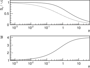
$M$ is greater than one for any appreciable background; and for large $\phi$, where $\tau=1/2$, $M$ can easily approach four as $M_{\tau=1/2}=(2+4\phi)/(1+\phi)$. The figure of merit from Eq. (9), using the optimal $\tau$ from Eq. (7), is graphed in fig. 8.

Figure 8: Upper plot — signal-to-noise ratio as a function of the background strength, $\phi$, from the complete singles method (solid line), and traditional methods (dotted line). Lower plot — figure of merit, $M$, from Eq. (9).

5 Validity of Chance Coincidence Equations

The effective live-time of a DAQ with significant readout or conversion times can be reduced by selectively triggering the system on a subset of events — perhaps even triggering on only the desired coincidence events. It is very difficult to apply Eq. (2) to such data sets. Suitably complete singles data sets should not include biases from the embedded coincidences, and ideally will not need any significant dead-time corrections. Therefore suitable data sets must be acquired using a non-selective trigger — in direct contradiction to a coincidence DAQ system with a large dead time.

Figure 9: Time difference between adjacent peaks in one lithium-glass detector. Upper curves (red online) show raw data, and lower curves (black online) show data after extra peaks are removed (see text).

A practical system to acquire a complete data set requires detectors and analog electronics with a relatively fast decay time to avoid pile up; and a dead-timeless DAQ. Flash analog-to-digital converters, with buffered multi-sample readout are ideally suited to this technique. Self triggered, on-board processing capabilities to identify and characterize peaks are not strictly required, but for many experiments will be the only practical way to obtain sufficient coincidence statistics.

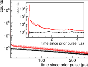
It is also necessary to ensure that a data set is not over-complete. Fig. 9 shows the distribution of the time differences between each peak and the previous for one of the lithium-glass detectors, over two different time scales. The firmware was configured to search for 200ns wide peaks, which is then the dead time, $t_{d}$. The decay constant of the time between adjacent cleaned peaks gives a count rate in the range of 5ks^-1. The product of the rate and the dead time is then about 0.001, which is sufficiently less than one that eqs. (1) and (2) are valid. Peaks at 1.8, 3.6, 5.4$\mu$s, … arise from the real change in the count rate during micro pulses. The raw data curves (upper curves, red online) show other structures and extraneous data for time differences less than 1.5$\mu$s. These arise predominantly from the peak searching algorithm re-triggering on fluctuations in the tail of large peaks, and must be removed by a suitable set of cuts on the data before applying Eq. (2) as in the lower curves (black online). The cuts should be applied before searching for coincidences, so that the background and signal are determined under the same conditions.

6 Conclusions

A method for measuring the background due to random coincidences in coincidence experiments has been presented. Although the method is based on a well known formula, we describe it as a new method, as it requires the use of a DAQ which can record all the singles data from which the coincidences are derived. The ability to take such data has only recently become practical as we now start to use waveform digitizers, which run continuously during time periods of interest. The dead times are now driven by detector response functions, rather than the digitization process or data recording process.

The method is very powerful, as it allows for true in situ background measurements, with a high degree of statistical certainty. The term in situ applies to the physical environment in which the detectors are located, and also to the application of the same data analysis cuts used to search for coincidences. The high statistical accuracy, even for experiments with a very small background, follows directly from an analysis procedure starting from sets of complete singles data from which the coincidences have been identified. This contrasts with traditional background measurement techniques, in which a separate set of coincidence measurements are made, with a change to the physical environment of the experiment, such that the possibility of forming a desirable coincidence has been removed.

A figure of merit for the method has been derived, based just on the statistical improvement compared to traditional methods of measuring backgrounds. Factors of up to four times more effective use of time are realistic. Impressive as this figure of merit is, it is still an underestimate of the power of the current technique. The current technique removes the systematic uncertainty in normalizing the background measurement, as the conditions are now known to be truly the same as during the foreground measurement. This systematic improvement in the background measurement has not been included in the figure of merit.

Furthermore, the algorithms used to extract the background are a form of analytic data reduction. They make no prior assumptions about the shape of the background, and do not involve any free parameters (in particular they do not use any type of fitting). As such, they are capable of reducing the data to determine very complicated background shapes, even while maintaining large figures of merit.

It is anticipated that the method will be of use to a large class of coincidence experiments, in which backgrounds cannot be fully eliminated. One such set of experiments is the measurement of the prompt fission neutron spectrum being performed at WNR/LANSCE. The method has been demonstrated using preliminary data sets from this project.

Appendix A Summing Over Similar Data Sets

As a practical matter, we must consider the application of Eq. (2) under the scenario of summing two data sets, taken sequentially, but otherwise under the same conditions. We use subscripts $1$ and $2$ to identify the two data sets.

Adding the background histograms directly gives

$$\gamma_{1+2}=\left(\frac{a_{1}b_{1}}{N_{1}}+\frac{a_{2}b_{2}}{N_{2}}\right)\\ \pm\sqrt{\frac{a_{1}b_{1}(a_{1}+b_{1})}{N_{1}^{2}}+\frac{a_{2}b_{2}(a_{2}+b_{2})}{N_{2}^{2}}},$$ (10)

whereas adding the singles histograms, and then calculating the background gives

$$\gamma_{1+2}=\frac{(a_{1}+a_{2})(b_{1}+b_{2})}{N_{1}+N_{2}}\\ \pm\sqrt{\frac{(a_{1}+a_{2})(b_{1}+b_{2})(a_{1}+a_{2}+b_{1}+b_{2})}{(N_{1}+N_{2})^{2}}}.$$ (11)

It is not immediately clear that eqs. (10) and (11) are the same result — indeed, at first glance they look very different. This dilemma is resolved by recalling that the number of counts in a data set is proportional to the time spent acquiring the data. Defining the detector dependent constant of proportionality as $k_{a}$ or $k_{b}$ so that $a=k_{a}N_{j}$ and $b=k_{b}N_{j}$, we find that eqs. (10) and (11) both reduce to the same result,

$$\gamma_{1+2}=k_{a}k_{b}(N_{1}+N_{2})\pm\sqrt{k_{a}k_{b}(k_{a}+k_{b})(N_{1}+N_{2})},$$ (12)

as desired.

Appendix B One bin of the projected 1D background

To determine a 1D time-difference histogram for the random coincidence background, it helps to make explicit the time dependence of the quantities in Eq. (2),

$$\gamma(t_{a},t_{b})=\frac{a(t_{a})b(t_{b})}{N}\pm\frac{1}{N}\sqrt{a(t_{a})b(t_{b})\big{(}a(t_{a})+b(t_{b})\big{)}}.$$ (13)

A single bin of $\beta(\delta_{t})$, is then a sum over independent elements of $\gamma(t_{a},t_{b})$ along the diagonal line $t_{b}=t_{a}+\delta_{t}$ (upper diagonal line, dark blue online, in fig. 10). The fluctuations from individual $\gamma(t_{a},t_{b})$ add in quadrature, so that

$$\begin{split}\beta(\delta_{t})&=\sum_{t_{a}}\gamma(t_{a},t_{a}+\delta_{t})\\ &=\frac{1}{N}\sum_{t_{a}}a(t_{a})b(t_{a}+\delta_{t})\pm\frac{1}{N}\sqrt{\sum\nolimits_{t_{a}}a(t_{a})b(t_{a}+\delta_{t})\big{(}a(t_{a})+b(t_{a}+\delta_{t})\big{)}}.\end{split}$$ (14)

Appendix C Correlations in the Projected 1D Background

Figure 10: Properties of $\gamma$ and $\beta$. $\beta(\delta_{t1})$ and $\beta(\delta_{t2})$ are sums of $\gamma$ along the upper and lower diagonal lines respectively (dark and light blue online). Correlations arise along vertical lines (red online) of constant $a(t_{a})$ and horizontal lines (orange online) of constant $b(t_{b})$.

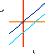
The background in a second bin of $\beta$, sums along a different set of $\gamma$ values, such as the lower diagonal line (light blue online) in fig 10. One term of $\beta(\delta_{t1})$ has the same value of $a(t_{a})$ as one term of $\beta(\delta_{t2})$. These terms lie on the intersection of the diagonal lines (blue online) in fig. 10 with the vertical line (red online) of constant $a(t_{a})$. There is a similar correlation, with a different term of $\beta(\delta_{t1})$, now along the horizontal line (orange online), for a constant $b(t_{b})$. In general, these two correlations occur for each term of $\beta(\delta_{t})$, and lead to a full a covariance matrix, ${\rm Cov}\beta(\delta_{t1},\delta_{t2})$.

Expressions for ${\rm Cov}\big{(}\beta(\delta_{t1}),\beta(\delta_{t2})\big{)}$ can be derived using the methods commonly described in text books (see e.g. [11]). However such an approach is overly cumbersome, as simplifications are easily found, reflecting the simple geometries of fig. 10.

First we observe that in Eq. (14), the partial derivatives $\partial\beta(\delta_{t})/\partial\gamma(t_{a},t_{a}+\delta_{t})$ are one (or zero), reflecting that the vertical (red online) and horizontal (orange online) lines intersect the upper diagonal (dark blue online) line of fig. 10 at only one point.

$${\rm Cov}\big{(}\beta(\delta_{t_{1}}),\beta(\delta_{t_{2}})\big{)}=\\ \sum_{t_{a_{1}}}\sum_{t_{a_{2}}}{\rm Cov}\big{(}\gamma(t_{a_{1}},t_{a_{1}}+\delta_{t1}),\gamma(t_{a_{2}},t_{a_{2}}+\delta_{t2})\big{)}.$$ (15)

Next we observe that frequently ${\rm Cov}\big{(}\gamma(t_{a_{1}},t_{a_{1}}+\delta_{1}),\gamma(t_{a_{2}},t_{a_{2}}+\delta_{2})\big{)}$ is zero, reflecting that the vertical (red online) and horizontal (orange online) lines of fig. 10 intersect the lower diagonal line (light blue online) at just two points. With these zeroes, the double summation is reduced to just one or two single summations:

$${\rm Cov}\big{(}\beta(\delta_{t_{1}}),\beta(\delta_{t_{2}})\big{)}=\\[6.0pt] \begin{cases}\displaystyle\sum_{t_{a}=1}^{\max(t_{a})}\!{\rm Cov}\big{(}\gamma(t_{a},t_{a}+\delta_{t_{1}}),\gamma(t_{a},t_{a}+\delta_{t_{2}})\big{)}&\text{\hbox to0.0pt{\hss if $\delta_{t_{1}}\!=\delta_{t_{2}}$,}}\\ \\ \displaystyle\sum_{t_{a}=1}^{\max(t_{a})}\!{\rm Cov}\big{(}\gamma(t_{a},t_{a}+\delta_{t_{1}}),\gamma(t_{a},t_{a}+\delta_{t_{2}})\big{)}&\text{\hbox to0.0pt{\hss otherwise.}}\\ \qquad+\!\!\!\!\displaystyle\sum_{t_{a}=\delta_{t_{2}}-\delta_{t_{1}}}^{\max(t_{a})}\!\!\!\!\!\!{\rm Cov}\big{(}\gamma(t_{a},t_{a}+\delta_{t_{1}}),\gamma(t_{a}+\delta_{t_{1}}\!-\delta_{t_{2}},t_{a}+\delta_{t_{1}})\big{)}\end{cases}$$ (16)

Finally we use

$${\rm Cov}\big{(}\gamma(t_{a_{1}},t_{b_{1}}),\gamma(t_{a_{2}},t_{b_{2}})\big{)}=\\[6.0pt] \begin{cases}\displaystyle{\frac{a(t_{a})b(t_{b})\big{(}a(t_{a})+b(t_{b})\big{)}}{N^{2}}}&\text{if $t_{a_{1}}\!=t_{a_{2}}\equiv t_{a}$, $t_{b_{1}}\!=t_{b_{2}}\equiv t_{b}$,}\\ \displaystyle{\frac{a(t_{a_{1}})a(t_{a_{2}})b(t_{b})}{N^{2}}}&\text{if $t_{a_{1}}\!\neq t_{a_{2}}$, $t_{b_{1}}\!=t_{b_{2}}\equiv t_{b}$,}\\ \displaystyle{\frac{a(t_{a})b(t_{b_{1}})b(t_{b_{2}})}{N^{2}}}&\text{if $t_{a_{1}}\!=t_{a_{2}}\equiv t_{a}$, $t_{b_{1}}\!\neq t_{b_{2}}$,}\\ 0&\text{otherwise,}\end{cases}$$ (17)

(obtained by standard techniques from Eq. (13)) to get the desired covariance matrix, in terms of the counts in the singles spectra:

$${\rm Cov}\big{(}\beta(\delta_{t_{1}}),\beta(\delta_{t_{2}})\big{)}=\\ \qquad\frac{1}{N^{2}}\sum_{t_{a}=1}^{\max(t_{a})}a(t_{a})b(t_{a}+\delta_{t})\big{(}a(t_{a}+\delta_{t1}-\delta_{t2})+b(t_{a}+\delta_{t1})\big{)}$$ (18)

References

- [1] G. F. Knoll, Radiation Detection and Measurement, 4th Edition, John Wiley & Sons, New York, 2010.
- [2] CAEN S.p., Viareggio, Italy, Charge Integration: Analog Vs. Digital, CAEN Application Note AN2503 (2010).
- [3] CAEN S.p., Viareggio, Italy, Digital Gamma Neutron discrimination with Liquid Scintillators, CAEN Application Note AN2506 (2012).
- [4] CAEN S.p., Viareggio, Italy, Digital Pulse Height Analyser—a digital approach to Radiation Spectroscopy, CAEN Application Note AN2508 (2011).
- [5] R. C. Haight, H. Y. Lee, T. N. Taddeucci, J. M. O’Donnell, B. A. Perdue, N. Fotiades, M. Devlin, J. L. Ullmann, A. Laptev, T. Bredeweg, M. Jandel, R. O. Nelson, S. A. Wender, M. C. White, C. Y. Wu, E. Kwan, A. Chyzh, R. Henderson, J. Gostic, The prompt fission neutron spectrum (pfns) measurement program at lansce, Nuclear Data Sheets 119 (2014) 205–208.
- [6] P. W. Lisowski, K. F. Schoenberg, The los alamos neutron science center, Nuclear Instruments and Methods in Physics Research Section A: Accelerators, Spectrometers, Detectors and Associated Equipment 562 (2) (2006) 910–914.
- [7] Teradyne, North Reading, MA, Defense and Aerospace Products, (formerly Ztec Instruments, Albuquerque, NM).
- [8] H. Y. Lee, T. N. Taddeucci, R. C. Haight, T. A. Bredeweg, A. Chyzh, M. Devlin, N. Fotiades, J. M. Gostic, R. A. Henderson, M. Jandel, E. Kwan, A. Laptev, R. O. Nelson, J. M. O’Donnell, B. A. Perdue, S. A. Wender, M. C. White, C. Y. Wu, Li-glass detector response study with a 252cf source for low-energy prompt fission neutrons, Nuclear Instruments and Methods in Physics Research Section A: Accelerators, Spectrometers, Detectors and Associated Equipment 703 (2013) 213–219.
- [9] C. Y. Wu, R. A. Henderson, R. C. Haight, H. L. Lee, T. N. Taddeucci, B. Bucher, A. Chyzh, M. Devlin, Fotiades, N., E. Kwan, J. M. O’Donnell, B. A. Perdue, J. L. Ullmann, A multiple parallel-plate avalanche counter for fission-fragment detection, Nuclear Instruments and Methods in Physics Research Section A: Accelerators, Spectrometers, Detectors and Associated Equipment 794 (2015) 76–79, (Availabled online 18 May 2015).
- [10] A. Enqvist, B. M. Wieger, L. Huang, M. Flaska, S. A. Pozzi, R. C. Haight, H. Y. Lee, E. Kwan, C. Y. Wu, Neutron-induced 235u fission spectrum measurements using liquid organic scintillation detectors, Physical Review C 86 (6) (2012) 064605.
- [11] G. Cowan, Statistical Data Analysis, Oxford Science Publications, Oxford, 1998.