Two-photon exchange correction to $2S$-$2P$ splitting in muonic helium-3 ions

Abstract

We calculate the two-photon exchange correction to the Lamb shift in muonic helium-3 ions within the dispersion relations framework. Part of the effort entailed making analytic fits to the electron-³He quasielastic scattering data set, for purposes of doing the dispersion integrals. Our result is that the energy of the 2$S$ state is shifted downwards by two-photon exchange effects by 15.14(49) meV, in good accord with the result obtained from a potential model and effective field theory calculation.

I Introduction

Lamb shift measurements in muonic helium are underway to measure the nuclear radius of the helium isotopes Antognini et al. (2011). The motivation comes from the proton radius puzzle, where the reported proton radii from measurements involving electrons and measurements involving muons have been different, with the difference exceeding five standard deviations Pohl et al. (2010); Antognini et al. (2013a). For reviews, see Pohl et al. (2013); Carlson (2015). One can hope to learn more about the root cause of the discrepancy by seeing if it persists, and how large its effect may be, with nuclei heavier than the proton. To this end, experiments have been performed to measure the $2S$-$2P$ Lamb shift energy splitting in muonic deuterium, ³He, and ⁴He Pohl et al. (2016); Antognini et al. (2016).

The experiments obtain the radius from the deviation of the energy splitting measured from the energy splitting calculated for a pointlike nucleus. To isolate the nuclear radius dependent term, it is crucial to know all the theory corrections that are large enough to affect the answer. The Lamb shift $2S$-$2P$ energy splitting is given as

$$\Delta E_{\rm Lamb}=\Delta E_{\rm QED}+\frac{m_{r}^{3}Z^{4}\alpha^{4}}{12}R_{E}^{2}+\Delta E_{\rm TPE}\,.$$ (1)

The accuracy of the QED term is not in question; reviews may be found in Borie (2012); Antognini et al. (2013b). The second term will yield the charge radius Karplus et al. (1952); Eides et al. (2001). The reduced mass $m_{r}$ is the usual

$$m_{r}=\frac{mM_{T}}{m+M_{T}},$$ (2)

where $m$ is the mass of the lepton and $M_{T}$ is the mass of the nucleus. The third term is the two-photon exchange (TPE) correction, the subject of this note for the case of muonic ³He, and given diagrammatically in Fig. 1.

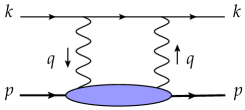
Figure 1: The diagram showing the two-photon exchange correction in muonic ³He.

An important question to consider at the outset is how accurately the two-photon correction needs to be calculated. An answer can be obtained from the uncertainty of the $\mathcal{O}(\alpha^{4})$ charge radius term as predicted using the charge radius measured in electron scattering. An analysis of world data for electron scattering on ³He Sick (2014) quoted $R_{E}(^{3}{\rm He})=1.973(14)$ fm. One can obtain a slightly better uncertainty limit by using the more extensive and more precise ⁴He electron scattering data together with isotope shift measurements from atomic spectroscopy. The charge radius of ⁴He is

$$R_{E}(^{4}{\rm He})=1.681(4){\rm\ fm}.$$ (3)

The isotope shift measures $\delta R_{E}^{2}=R_{E}^{2}(^{3}{\rm He})-R_{E}^{2}(^{4}{\rm He})$. Unfortunately, the three existing measurements are not in agreement,

$$\delta R_{E}^{2}=\left\{\begin{array}[]{ll}1.066(4){\rm\ fm}^{2}&{\rm\ Ref.}~{}[13]\\ 1.074(4){\rm\ fm}^{2}&{\rm\ Refs.}~{}[14,15]\\ 1.028(11){\rm\ fm}^{2}&{\rm\ Ref.}~{}[16]\end{array}\right.$$ (7)

These yield $R_{E}(^{3}{\rm He})=1.9728(36)$, $1.9748(36)$, and $1.9631(44)$ fm, respectively, adding uncertainties in quadrature. To exclude either of the above determinations by three respective standard deviations via a Lamb shift measurement, the second term in Eq. (1) should be determined with an accuracy of about $1.5$ meV. Hence, the requirement to the precision of the third term of that equation, the TPE correction is to be below $1.5$ meV. Its size, as we shall see, is about $15$ meV, so as a fraction one needs an accuracy better than $10\%$. One should bear in mind that even when this precision goal is met, the accuracy of the TPE calculation will remain by far the main limitation of the charge radius extraction, since the experimental accuracy of order $0.07$ meV or better Antognini et al. (2011) is expected.

An additional numerical benchmark follows from what may happen if beyond the standard model (BSM) explanations of the proton radius are correct Tucker-Smith and Yavin (2011); Batell et al. (2011); Carlson and Rislow (2012). In this scenario, the muonic $2S$-$2P$ energy deficit that was attributed to a smaller proton radius is instead attributed to a muon specific BSM force. For purposes of benchmarking, consider a BSM model where the new exchange particle couples on the hadron side in proportion to the electric charge, like a dark photon that is muon specific on the lepton side (for an alternative scenario where its couplings to the proton and the neutron allowed arbitrary values, see Ref. Liu et al. (2016)). Also consider, at least at the outset, that the new force is short range for both $\mu$-H and $\mu$-³He. This requires that the new exchange particle is heavy enough, and a few $10$’s of MeV will suffice. Then the $330\,\mu$eV energy deficit for muonic hydrogen scales to

$$\Delta E_{\rm BSM}^{\mu\,^{3}{\rm He}}=6.0{\rm\ meV},$$ (8)

for the $2S$-$2P$ splitting. The bulk of the scaling comes from a $Z^{4}$ factor and the remainder from differences in the reduced mass. Thus also from considering the scale of possible BSM effects, a $5$-$10\%$ calculation of the TPE correction is useful and relevant. (A lower mass BSM exchange particle will reduce the value obtained for $\Delta E_{\rm BSM}^{\mu\,^{3}{\rm He}}$.)

An accurate potential model calculation of the TPE is already available Nevo Dinur et al. (2016); Hernandez et al. (2016), so one may ask why another estimate is useful? The answer is that the result is very important for the study of the proton radius puzzle, so that another calculation using a very different technique is worth doing and reporting. Our fully relativistic calculation is directly phenomenological, using dispersion theory to connect electron-³He elastic and inelastic scattering data to quantities that enter the evaluation of the TPE effect. The already available calculation is nonrelativistic with relativistic corrections and is based on nuclear potential models. The potentials are either a classical one, the AV18 potential abetted with three-nucleon forces, or a chiral effective field theory potential, also with three-nucleon forces added to the two-nucleon ones. We will see that the dispersive and the nuclear potential model calculations corroborate each other.

Dispersive evaluations of the TPE correction have been carried out for muonic hydrogen Pachucki (1999); Martynenko (2006); Carlson and Vanderhaeghen (2011); Birse and McGovern (2012); Gorchtein et al. (2013) and muonic deuterium Carlson et al. (2014). For $\mu$-H they represent the state of the art and are accepted as such Antognini et al. (2013a). Other methods evaluating TPE in $\mu$-H Nevado and Pineda (2008); Alarcon et al. (2014); Peset and Pineda (2015) are not yet equivalent in accuracy. The deuterium situation is different. The deuteron is loosely bound, easily polarized, and can be broken up with just a bit over $2$ MeV energy transfer. The relevant integrals for the dispersive evaluation are weighted toward low-energy transfer and low-momentum transfer. Electron-deuteron scattering data is currently sparse in these regions, and the outcome is a not very stringent $35\%$ uncertainty in the dispersive result Carlson et al. (2014). One must rely instead on nuclear potential model evaluations Pachucki (2011); Friar (2013); Hernandez et al. (2014); Pachucki and Wienczek (2015) (we refer the reader to a summary of theoretical calculations in Ref. Krauth et al. (2016)). Helium nuclei are tightly bound compared to the deuteron, and more than $5$ MeV energy transfer is required for ³He disintegration. It is enough to make a significant difference. There are more data points than for the deuteron in the range where the necessary integrals have their main support, and the higher threshold for the low energy weighting makes the numerical results smaller. We find that for ³He we can meet the accuracy goal.

II Calculation

The diagram that contains the nuclear and hadronic structure-dependent ${\cal O}(\alpha^{5})$ correction to the Lamb shift is shown in Fig. 1. The lower part of the diagram, the blob containing nuclear and hadronic structure dependence is encoded in the forward virtual Compton tensor,

$$T^{\mu\nu}=\frac{i}{8\pi M_{T}}\int d^{4}x\,e^{iqx}\langle p|T\,j^{\mu}(x)j^{\nu}(0)|p\rangle$$ (9)

$$=\left(-g^{\mu\nu}+\frac{q^{\mu}q^{\nu}}{q^{2}}\right)T_{1}(\nu,Q^{2})+\frac{\hat{p}^{\mu}\hat{p}^{\nu}}{M_{T}^{2}}T_{2}(\nu,Q^{2}),$$

where $\hat{p}^{\mu}=p^{\mu}-\frac{p\cdot q}{q^{2}}q^{\mu}$, $Q^{2}=-q^{2}$, $\nu=(p\cdot q)/M_{T}$ and $M_{T}$ is the ³He mass. A target spin average is implied. Following Carlson and Vanderhaeghen (2011), we can write the contribution of the two-photon exchange diagram to the $n\ell$ energy level as

$$\Delta E_{n\ell}=\frac{8\alpha^{2}m}{\pi}\phi^{2}_{n\ell}(0)\int d^{4}Q$$ (10)

$$\times\frac{(Q^{2}+2Q_{0}^{2})T_{1}(iQ_{0},Q^{2})-(Q^{2}-Q_{0}^{2})T_{2}(iQ_{0},Q^{2})}{Q^{4}(Q^{4}+4m^{2}Q_{0}^{2})},$$

where a Wick rotation $q_{0}=iQ_{0}$ was made, and $\phi^{2}_{n\ell}(0)=\mu_{r}^{3}(Z\alpha)^{3}/(\pi n^{3})\delta_{\ell 0}$. The amplitudes $T_{1,2}(\nu,Q^{2})$ are even functions of $\nu$ and their imaginary parts are related to the spin-independent structure functions of lepton-³He scattering,

$${\rm Im}T_{1}(\nu,Q^{2}) = \frac{1}{4M_{T}}F_{1}(\nu,Q^{2}),$$

$${\rm Im}T_{2}(\nu,Q^{2}) = \frac{1}{4\nu}F_{2}(\nu,Q^{2}).$$ (11)

Before writing the dispersion relation, we will give the Born terms, which are obtained from the elastic box and crossed box version of Fig. 1 and ³He electromagnetic vertex,

$$\Gamma^{\mu}(q)=F_{D}(Q^{2})\gamma^{\mu}+F_{P}(Q^{2})i\sigma^{\mu\alpha}\frac{q_{\alpha}}{2M_{T}},$$ (12)

with $F_{D,P}$ the Dirac and Pauli form factors of ³He and $q$ the momentum of an incoming photon. To disambiguate, we will use $F_{D,P}^{p,n}$ notation for the proton and neutron Dirac and Pauli form factors, respectively. The Born terms are

$$T_{1}^{B}(q_{0},Q^{2}) =\frac{Z^{2}}{4\pi M_{T}}\left\{\frac{Q^{4}G_{M}^{2}(Q^{2})}{(Q^{2}-i\epsilon)^{2}-4M_{T}^{2}q_{0}^{2}}-F_{D}^{2}(Q^{2})\right\}\,,$$

$$T_{2}^{B}(q_{0},Q^{2}) =\frac{Z^{2}M_{T}Q^{2}}{\pi(1+\tau_{T})}\frac{G_{E}^{2}(Q^{2})+\tau_{T}G_{M}^{2}(Q^{2})}{(Q^{2}-i\epsilon)^{2}-4M_{T}^{2}q_{0}^{2}}\,.$$ (13)

Nuclear electric and magnetic Sachs form factors are defined in the standard way,

$$G_{E} = F_{D}-\tau_{T}F_{P},$$

$$G_{M} = F_{D}+F_{P},$$ (14)

and $\tau_{T}=Q^{2}/(4M_{T}^{2})$. The Born terms are useful for correctly obtaining the imaginary parts of the nucleon pole terms, but not reliable in general, since the given vertex assumes the incoming and outgoing nucleons are both on shell.

We also define

$$\overline{T}_{1,2}(\nu,Q^{2})=T_{1,2}(\nu,Q^{2})-T_{1,2}^{\rm pole}(\nu,Q^{2}),$$ (15)

where $T_{1,2}^{\rm pole}$ are the pole parts of the Born amplitudes. For future use, the non-pole $\overline{T}_{1}(0,Q^{2})$ amplitude can be written as a term visible in the Born term plus a term proportional to $Q^{2}$ at small $Q^{2}$,

$$\overline{T}_{1}(0,Q^{2})=-\frac{Z^{2}F_{D}^{2}(Q^{2})}{4\pi M_{T}}+\frac{Q^{2}}{e^{2}}\beta_{M}^{{}^{3}{\rm He}}(Q^{2})\,,$$ (16)

where $\beta_{M}^{{}^{3}{\rm He}}(0)=\beta_{M}^{{}^{3}{\rm He}}$ is the magnetic polarizability of ³He.

Given the known high-energy behavior of the structure functions, the two amplitudes obey the following form of dispersion relation,

$${\rm Re\,}\overline{T}_{1}(q_{0},Q^{2}) =\overline{T}_{1}(0,Q^{2})+\frac{q_{0}^{2}}{2\pi M_{T}}\int\limits_{\nu_{\rm th}}^{\infty}\frac{d\nu F_{1}(\nu,Q^{2})}{\nu(\nu^{2}-q_{0}^{2})},$$

$${\rm Re\,}\overline{T}_{2}(q_{0},Q^{2}) =\frac{1}{2\pi}\int\limits_{\nu_{\rm th}}^{\infty}\frac{d\nu F_{2}(\nu,Q^{2})}{\nu^{2}-q_{0}^{2}},$$ (17)

where the integrals are evaluated in the principle value sense, and $\nu_{\rm th}$ is the inelastic threshold.

We divide the contribution to the energy shift of the $S$-state into three physically distinct terms that originate from the subtraction term $\overline{T}_{1}(0,Q^{2})$, the nucleon pole, and finally all excited intermediate states that may couple to $\gamma N$, respectively

$$\Delta E_{nS} = \Delta E_{nS}^{\rm subt}+\Delta E_{nS}^{\rm el}+\Delta E_{nS}^{\rm inel}.$$ (18)

with

$$\Delta E_{nS}^{\rm subt} =\frac{4\pi\alpha^{2}}{m}\phi^{2}_{n0}(0)$$

$$\times\int_{0}^{\infty}\frac{dQ^{2}}{Q^{2}}\frac{\gamma_{1}(\tau_{l})}{\sqrt{\tau}_{l}}\left[\overline{T}_{1}(0,Q^{2})-\overline{T}_{1}(0,0)\right],$$ (19)

$$\Delta E_{nS}^{\rm el}=\alpha^{2}Z^{2}\phi^{2}_{n0}(0)\int_{0}^{\infty}\frac{dQ^{2}}{Q^{2}}\Bigg{\{}\frac{16mM_{T}}{(M_{T}+m)Q}G^{\prime}_{E}(0)$$

$$-\frac{m}{M_{T}(M_{T}^{2}-m^{2})}\Bigg{[}\!\!\left(\frac{\gamma_{1}(\tau_{T})}{\sqrt{\tau}_{T}}-\frac{\gamma_{1}(\tau_{l})}{\sqrt{\tau}_{l}}\right)\!\!\left(G_{M}^{2}-1\right)$$

$$\qquad-\left(\frac{\gamma_{2}(\tau_{T})}{\sqrt{\tau}_{T}}-\frac{\gamma_{2}(\tau_{l})}{\sqrt{\tau}_{l}}\right)\frac{G_{E}^{2}-1+\tau_{T}\left(G_{M}^{2}-1\right)}{\tau_{T}(1+\tau_{T})}\Bigg{]}\Bigg{\}},$$ (20)

$$\Delta E_{nS}^{\rm inel}=-\frac{2\alpha^{2}}{mM_{T}}\phi^{2}_{n0}(0)\int_{0}^{\infty}\frac{dQ^{2}}{Q^{2}}\int_{\nu_{\rm th}}^{\infty}\frac{d\nu}{\nu}$$

$$\times\left[\tilde{\gamma}_{1}(\tau,\tau_{l})F_{1}(\nu,Q^{2})+\frac{M_{T}\nu}{Q^{2}}\tilde{\gamma}_{2}(\tau,\tau_{l})F_{2}(\nu,Q^{2})\right].$$ (21)

We introduced $\tau_{l}=Q^{2}/(4m_{\ell}^{2})$, $\tau=\nu^{2}/Q^{2}$, and the auxiliary functions,

$$\gamma_{1}(\tau) \equiv (1-2\tau)\sqrt{1+\tau}+2\tau^{3/2}$$

$$\gamma_{2}(\tau) \equiv (1+\tau)^{3/2}-\tau^{3/2}-\frac{3}{2}\sqrt{\tau}$$

$$\tilde{\gamma}_{1}(\tau,\tau_{l}) \equiv \frac{\sqrt{\tau}_{l}\gamma_{1}(\tau_{l})-\sqrt{\tau}\gamma_{1}(\tau)}{\tau_{l}-\tau}$$

$$\tilde{\gamma}_{2}(\tau,\tau_{l}) \equiv \frac{1}{\tau_{l}-\tau}\left(\frac{\gamma_{2}(\tau)}{\sqrt{\tau}}-\frac{\gamma_{2}(\tau_{l})}{\sqrt{\tau}_{l}}\right).$$ (22)

Furthermore, we have subtracted two-photon exchange terms in $\Delta E^{\rm el}$ that are already included in a bound state calculation. The “$-1$”s come from iterations within the basic wave equation calculation that gives the bound state, which is done for a pointlike nucleus, and the $G^{\prime}_{E}$ term removes the iteration of the lowest order nuclear radius term seen in Eq. (1). Recall that by definition,

$$R_{E}^{2}=-6G^{\prime}_{E}(0).$$ (23)

II.1 Elastic contribution

Using the form factor parametrization obtained by Amroun et al. Amroun et al. (1994) and Sick Sick (2008) in the sum-of-gaussians form we obtain:

$$\Delta E_{2S}^{el} = -10.93\,{\rm meV},$$ (24)

in an excellent agreement with a dedicated extraction of the Zemach radius in Ref. Sick (2014) from scattering data, which leads to the energy shift

$$\Delta E_{2S}^{el} = -10.87(27)\,{\rm meV},$$ (25)

where we note a significant $\sim$3% uncertainty, and we will use it as an uncertainty estimate for our evaluation.

Krutov et al. Krutov et al. (2015) used an exponential form factor $G_{E}=\exp[-R_{E}^{2}Q^{2}/6]$, leading to an estimate of the elastic contribution,

$$\Delta E_{2S}^{el} = -10.28\,{\rm meV},$$ (26)

considerably smaller than what one obtains by using phenomenological form factors which fit the data better. Similarly, the elastic contribution obtained using the deuteron form factors of De Vries et al. (1987) is also notably smaller than the value we quote above, but De Vries et al. (1987) did not have available the later data obtained by Amroun et al. Amroun et al. (1994).

II.2 Inelastic contribution

We separate the inelastic contributions into two regions, the quasieleastic or nuclear region, where the final states are either three nucleons or a deuteron plus a proton, and the pion production or nucleon region. In practice, we separate these regions at the pion production threshold. Thus, we write the inelastic contributions as two parts,

$$\Delta E^{\rm inel}_{nS}=\Delta E^{\rm nuclear}_{nS}+\Delta E^{\rm nucleon}_{nS},$$ (27)

which we will treat in the next two subsections.

II.2.1 Nuclear polarizability contribution

The bulk of the data in this region has been tabulated by Benhar, Day, and Sick Benhar et al. (2006, 2008). This tabulation has 83 data sets categorized by incoming electron energy and electron scattering angle. To this tabulation, we add the three $180^{\circ}$ data sets Jones et al. (1979); Chertok et al. (1969).

For purposes of evaluating the integrals, we make analytic fits to this data. Details are given in the Appendix. In brief, we started with functional forms motivated by a Fermi gas model of the nucleus, which was called to our attention by superscaling studies of electron-nucleus scattering Maieron et al. (2002); Bosted and Mamyan (2012); Bodek et al. (2014). We modified the forms with additional parameters so that we could fit the lower energy and lower momentum transfer data crucial to the present calculation. We paid special attention to the photoproduction ($Q^{2}=0$) and near photoproduction data, and added extra terms to ensure these regions were well represented.

Samples of the fits are shown in Fig. 2, with $\pm 10\%$ error bands indicated. At the $\pm 10\%$ level, the fits are overall good, and if the uncertainties in both the data and the fits are purely statistical, the uncertainty in the integrals is much less than $10\%$.

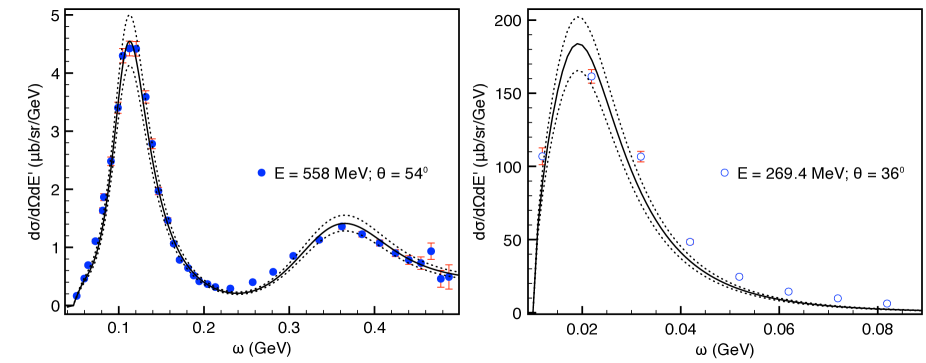
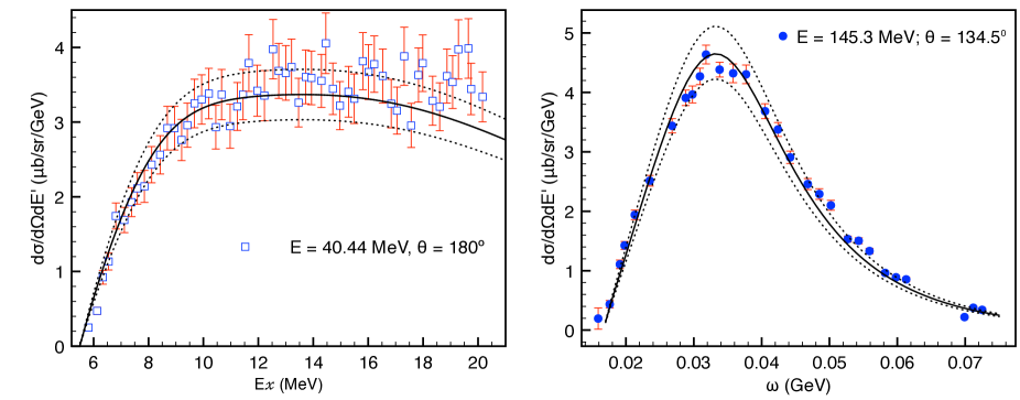
Figure 2: Parametrization defined in Eqs. (A-51) compared to the experimental data in forward (upper panels) and backward (lower panels) kinematics. Data are from Ref. Jones et al. (1979) (empty squares), Ref. Marchand et al. (1985) (solid circles), and Ref. Dow et al. (1988) (empty circles). Dotted curves in all three panels indicate the 10% uncertainty band. The spectrum in the lower left panel is shown as function of excitation energy $E_{x}$ in units of MeV, and as function of photon energy in units of GeV otherwise.

The result for the quasielastic or nuclear part of the inelastic contributions is

$$\Delta E^{\rm nuclear}=-5.50\,(40){\rm\ meV}.$$ (28)

The uncertainty on this number is explained in appendix.

II.2.2 Intrinsic nucleon polarizability contribution

The contributions from the nucleon region, where we have energy sufficient for nucleon breakup, is separable from other contributions, and the results of this subsection can be taken and combined with calculations where the other contributions are calculated in ways different from what we have done.

We use modern helium-3 virtual photoabsorption data that were parametrized in terms of resonances plus non-resonant background Bosted and Mamyan (2012); Bodek et al. (2014) that capitalizes on the free proton and neutron fits of Refs. Bosted and Christy (2008); Christy and Bosted (2010) with a Fermi-smearing effect built in. Since the integration over the energy extends beyond the validity of the fit of Refs. Bosted and Christy (2008); Christy and Bosted (2010), we supplement the correct high-energy behavior by adopting a Regge-behaved background, specified in our previous work for the deuteron case, Carlson et al. (2014), and adjusted for the case of the helium target. The result of the integration is

$$\Delta E_{2S}^{\rm nucleon} = -0.306(15)\,{\rm meV}.$$ (29)

Summing the nuclear and nucleon polarizability contributions leads to

$$\Delta E_{2S}^{\rm inel}=-5.81(40){\rm\ meV},$$ (30)

with the uncertainties added in quadrature.

II.3 Subtraction contribution

The subtraction function $T_{1}(0,Q^{2})$ is generally unknown. We need it at nonnegative $Q^{2}$. Excepting $Q^{2}=0$, this is unphysical kinematics and not directly related to scattering data. Instead we obtain it from a sum rule Gorchtein (2015) based on the dispersion relation for $T_{1}$ and several additional observations.

The sum rule is fully explained in Gorchtein (2015). The dispersion relation for $T_{1}$ is analyzed and approximated after observing that: firstly, the imaginary part Im$\,T_{1}(\nu,Q^{2})\propto F_{1}(\nu,Q^{2})$ in the quasielastic region becomes quite small beyond a certain value of $\nu$ for a given $Q^{2}$, creating a “gap region” between it and the onset of the pion production region. Secondly, there is a separation of scales, in that the gap region is quite broad. Thirdly, for high energies, the binding effects are relatively small and we can, at least within integrals, treat the ³He structure functions as just that for two protons plus one neutron. Then combing the dispersion relation for ³He with the corresponding dispersion relations for the proton and neutron, one can obtain

$$\overline{T}_{1}(0,Q^{2})=\frac{1}{2\pi M_{T}}\int\limits_{\nu_{min}(Q^{2})}^{\nu_{max}(Q^{2})}\frac{d\nu}{\nu}F_{1}(\nu,Q^{2})$$

$$\;\;\;+\frac{Q^{2}}{e^{2}}(2\beta_{M}^{p}(Q^{2})+\beta_{M}^{n}(Q^{2}))-\frac{2F_{D}^{p\,2}+F_{D}^{n\,2}}{4\pi M_{p}}.$$ (31)

Here, $\nu_{\rm max}(Q^{2})$ is the upper limit of the region where the quasielastic structure function is large, and $\beta_{M}^{p,n}(Q^{2})$ are the nucleon analogs of $\beta_{M}^{{}^{3}{\rm He}}(Q^{2})$ described earlier, normalized at $Q^{2}=0$ to the experimentally determined magnetic polarizabilities of the proton and neutron, respectively.

A test of the sum rule is to evaluate its $Q^{2}=0$ limit, using the known result for $\overline{T}_{1}(0,0)$ to obtain,

$$NZ=2=2\int_{\nu_{min}}^{\nu_{max}}\frac{d\nu}{\nu}F_{1}(\nu,0)\,,$$ (32)

which is the Bethe-Levinger sum rule Levinger and Bethe (1950). Using the structure function fits described in the Appendix and integrating to $30$ MeV above threshold gives

$$2\int_{\nu_{min}}^{\nu_{min}+30{\rm MeV}}\frac{d\nu}{\nu}F_{1}(\nu,0)=1.65\,.$$ (33)

Integrating to $60$ MeV above threshold gives $1.78$. The sum rule appears to work at the $15\%$ level or better.

Using the sum rule to obtain $T_{1}(0,Q^{2})$ and $T_{1}(0,0)$ for the subtraction term energy, Eq. (II), leads to

$$\Delta E_{2S}^{\rm subt}=\left(1.39+0.21\right){\rm\,meV}=1.60{\rm\ meV},$$ (34)

where the separated terms are for the nuclear and nucleon contributions, respectively. We took the nucleon polarizabilities from the PDG average Olive et al. (2014),

$$\beta_{M}^{p}=2.5(0.4)\cdot 10^{-4}\,{\rm fm}^{3}, \beta_{M}^{n}=3.7(2.0)\cdot 10^{-4}\,{\rm fm}^{3},$$ (35)

and took the $Q^{2}$ dependence for $\beta_{M}^{p,n}(Q^{2})$ following Birse and McGovern (2012).

The uncertainty in the subtraction term contribution to the Lamb shift comes from two sources which we refer to as statistical and systematic. The statistical one is due to the finite precision and kinematical coverage of the data used for evaluating the sum rule integral. This uncertainty should be considered jointly with the uncertainty of the inelastic contribution because the same parametrization of the data enters there. An important effect is a partial cancellation of the subtraction term and the inelastic $F_{1}$ contribution, which leads to a reduced uncertainty. We address this uncertainty in detail in the appendix.

The systematic uncertainty is due to the use of the approximate sum rule for the subtraction function. To assess its uncertainty, we note that the derivation of the sum rule Gorchtein (2015) relies on the assumption of the large gap between the nuclear and nucleon excitation spectra, and of the dominance of the nuclear contributions over the hadronic ones. A comparison of the nuclear and nucleonic contributions to Eq. (31) reveals that they become of similar size starting from $Q^{2}\approx(0.3$ GeV)². We assign a conservative 100% uncertainty to the contribution coming from $Q^{2}$ beyond this value, and find

$$(\Delta E_{2S}^{\rm subt,nuclear})_{Q^{2}>0.1\,{\rm GeV}^{2}}=0.11\,{\rm meV},$$ (36)

which leads us to the final estimate of the subtraction term,

$$\Delta E_{2S}^{\rm subt}=1.60(12)\,{\rm meV}.$$ (37)

where we added the uncertainty of the nucleon and nuclear contributions in quadrature.

Of palpable interest is the numerical value of the ³He polarizability $\beta_{M}^{{}^{3}{\rm He}}$, which can be obtained from the derivative of the sum rule at $Q^{2}=0$ and the relation in Eq. (16). This leads to

$$\beta_{M}^{{}^{3}{\rm He}} =\frac{2\alpha}{M_{T}}\int_{\nu_{0}}^{\nu_{max}}\frac{d\nu}{\nu}\frac{dF_{1}^{{}^{3}{\rm He}}}{dQ^{2}}(\nu,0)-\frac{Z^{2}\alpha}{3M_{T}}\big{(}R_{E}^{{}^{3}{\rm He}}\big{)}^{2}$$

$$+\frac{\alpha}{3M_{p}}\left[2R_{Ep}^{2}+R_{En}^{2}\right]+2\beta_{M}^{p}+\beta_{M}^{n}\,.$$ (38)

Using the $F_{1}$ parametrizations from the Appendix, the ³He charge radius 1.956 fm, the known nucleon radii, and the values for $\beta_{M}^{p,n}$ from Ref. Hagelstein et al. (2016), we obtain

$$\beta_{M}^{{}^{3}{\rm He}}=5.7\times 10^{-3}\,{\rm fm}^{3}.$$ (39)

Since the value of the ³He magnetic polarizability is unknown, we stress that this is a prediction to be tested in the future, either experimentally or in an EFT calculation. Using the spread in the values of $\beta_{M}^{p,n}$ from different analyses and the uncertainty in the $Q^{2}$-slope of $F_{1}$ at low $Q^{2}$, we conjoin an uncertainty estimate,

$$\beta_{M}^{{}^{3}{\rm He}}=5.7(0.5)\times 10^{-3}\,{\rm fm}^{3}.$$ (40)

In contrast, a recent lattice calculation Chang et al. (2015) gives a much smaller value $\beta^{{}^{3}{\rm He}}_{M}=5.4(2.2)\times 10^{-4}\,{\rm fm}^{3}$, obtained in conjunction with a pion mass of about $806$ MeV. The same reference also suggests $\beta^{d}_{M}=4.4(1.5)\times 10^{-4}\,{\rm fm}^{3}$, more than two orders of magnitude smaller than the EFT prediction of about $0.07$ fm³ Friar and Payne (1997); Chen et al. (1998).

In view of this inconclusive situation with the value of $\beta_{M}$, we wish to emphasize that as far as the nuclear polarizability contribution to the Lamb shift is concerned, it is practically insensitive to the value of $\beta_{M}$. The reason for that is the cancellation between the inelastic and subtraction contributions, both coming from the transverse Compton amplitude $T_{1}$. The sum rule that we use here ensures that whenever the parametrization of the transverse QE data changes, this change is also propagated in the subtraction function, so that the net effect is small. This is in accord with the general expectation of smallness of the magnetic polarizability effect on Lamb shift, e.g. in potential model calculations.

III Results and discussion

The result of our phenomenological, dispersion relation based, calculation is summarized in Table I. The overall result is that the 2$S$ state has its energy shifted due to two-photon exchange by an amount

$$\Delta E_{2S}=-15.14(49){\rm\,meV}.$$ (41)

The uncertainty limit is small enough, exceeding the criterion set out in the introduction by a factor of 3.

Contribution	This work	Refs. [21,22]
Elastic	$-10.93(27)$	$-10.49(24)$
$\delta_{\rm Zem}^{N}$		$-0.52(3)$
Inelastic	$-5.81(40)$	$-4.45(21)$
Nuclear	$-5.50(40)$	$-4.17(17)$
Nucleon	$-0.31(2)$	$-0.28(12)$
Subtraction	$1.60(12)$
Nuclear	$1.39(12)$
Nucleon	$0.21(3)$
Total TPE	$-15.14(49)$	$-15.46(39)$

Table I: Individual contributions to $\Delta E_{2S}$ from two-photon exchange in $\mu$-³He, in units of meV.

To facilitate the comparison with other work, we included in Table I results from the recent work of Ref. Nevo Dinur et al. (2016). We shall make some comparison, even though that calculation is very different from ours, so that comparisons of any but the total may be inexact. There, the nuclear elastic contribution,

$$\Delta E_{2S}^{el} = -10.52(24)\,{\rm meV},$$ (42)

is somewhat lower than our full elastic contribution, but once the nucleon Zemach correction $\delta_{\rm Zem}^{N}$ listed in the rightmost column in Table I is added to it, their full result,

$$\Delta E_{2S}^{el,\,tot.} = -11.01(25)\,{\rm meV},$$ (43)

is close to ours.

The same reference calculated the nuclear polarizability contribution using potential models and effective field theory. For a reasonable comparison, we should confront the sum of nuclear, nucleon polarizabilities, with the sum of the total inelastic and total subtraction contributions obtained in this work,

$$-4.45(21)\;{\rm Refs.\ }[21,22] {\rm vs.} -4.21(40)\;{\rm This\;work},$$

where various uncertainties were added in quadrature. The two results closely agree.

We conclude by noting that the main limitation of our calculation of the TPE effect on the Lamb shift in muonic He-3 is the availability and precision of the quasielastic data at low $Q^{2}$ and forward angles. To assess the improvability of our result, we study the impact of possible measurements of the inclusive differential cross section for electron-³He scattering in the quasielastic regime with the new MESA accelerator in Mainz. We assume a generic 5% accuracy of the data, feasible for MESA with the laboratory energy $E=110$ MeV and scattering angle $20^{\circ}\leq\theta\leq 30^{\circ}$, and list the projected accuracy in determining the parameter $a_{2}$ entering the parameterization of Eq. (49), as well as that of the nuclear polarizability and the full TPE contributions to the Lamb shift in $\mu\,^{3}$He atoms in Table II. At the moment, the lowest available momentum transfer at forward angles is $Q^{2}=0.0091$ GeV² from the 110 MeV, $54^{\circ}$ data set of Ref. Dow et al. (1988), shown in Table II. We notice from Table II that a future 5 % measurement of $d\sigma/d\Omega$ at MESA around $\theta\approx 30^{\circ}(20^{\circ})$ will reduce the total uncertainty of the polarizability contribution by a factor of $2$ ($4$) respectively. The resulting TPE contribution will then be mainly limited by the present knowledge of the elastic contribution, which can also be improved by such future measurements.

Kinematics	$\delta a_{2}$	$\delta(\Delta E_{\rm 2S}^{\rm nuclear})$	$\delta(\Delta E_{\rm 2S}^{\rm TPE})$
$E=110$ MeV
$\theta=54^{\circ}$	$\pm 0.014$	$0.40$ meV	$0.49$ meV
$\theta=30^{\circ}$	$\pm 0.0075$	$0.21$ meV	$0.35$ meV
$\theta=25^{\circ}$	$\pm 0.0055$	$0.16$ meV	$0.33$ meV
$\theta=20^{\circ}$	$\pm 0.0040$	$0.11$ meV	$0.30$ meV

Table II: The impact of possible 5% measurements of $d\sigma/d\Omega$ in the quasielastic kinematics at MESA with laboratory energy $E=110$ MeV and scattering angle $20^{\circ}\leq\theta\leq 30^{\circ}$ for constraining the parameter $a_{2}$ and the nuclear polarizability and full TPE contributions to the Lamb shift in muonic ³He. The upper row shows the current situation with the available data.

Appendix A Fitting the quasielastic data

We make use of the quasi elastic data collected on the Donal Day’s web archive, which may be found through Benhar et al. (2006). The specific data that have the biggest impact on this calculation are Retzlaff et al. (1994); Jones et al. (1979); Marchand et al. (1985); Dow et al. (1988) which extend from the quasielastic threshold to above the pion production threshold, and for 0.005 GeV${}^{2}\leq Q^{2}\leq 0.7$ GeV².

The full nuclear structure functions are parameterized here in two parts,

$$F_{1,2}(\nu,Q^{2})=F_{1,2}^{\rm QE}(\nu,Q^{2})+F_{1,2}^{\rm real}(\nu,Q^{2})\,.$$ (45)

We use the super scaling parametrization of quasi elastic data according to Maieron et al. (2002); Bodek et al. (2014); Bosted and Mamyan (2012) with additional adjustments to provide a better description of the data with an emphasis on the low energy and low $Q^{2}$ region. For the single-nucleon structure functions we use the following representation,

$$F_{1}^{\rm QE} =\frac{Q^{2}}{|\vec{q}\,|}\bar{G}_{M}^{2}S_{1}(\nu,Q^{2})$$

$$F_{2}^{\rm QE} =\frac{\nu Q^{4}}{M_{T}|\vec{q}\,|^{5}}\frac{\bar{G}_{E}^{2}+\tau_{p}\bar{G}_{M}^{2}}{1+\tau_{p}}(2M_{p}+\nu)^{2}S_{2}(\nu,Q^{2}),$$ (46)

where $\bar{G}_{E,M}^{2}=2(G_{E,M}^{p})^{2}+(G_{E,M}^{n})^{2}$, and the functions $S_{i}(\nu,Q^{2})$ are defined as

$$S_{i}(\nu,Q^{2})=F(\psi^{\prime})F_{P}(|\vec{q}\,|)\!\left[1-\left(\frac{\nu_{thr}}{\nu}\right)^{3}\right]^{\alpha_{i}}\!\!\!\sqrt{\frac{\nu_{thr}}{\nu}}f_{i}^{QE}(Q^{2}),$$ (47)

which contain the superscaling variable $\psi^{\prime}$, the super scaling function $F(\psi^{\prime})$, and the Pauli suppression factor $F_{P}$, all as described in Bodek et al. (2014). Above, $\vec{q}\,^{2}=\nu^{2}+Q^{2}$, $\tau_{p}={Q^{2}}/(4m_{p}^{2})$, $\nu_{\rm thr}=\epsilon_{T}+Q^{2}/(2M_{T})$, with

$$\epsilon_{T} =S_{p}+\frac{S_{p}^{2}}{2M_{T}}=M_{d}+M_{p}-M_{T}+\frac{S_{p}^{2}}{2M_{T}}$$

$$=5.493{\rm\,MeV}\,,$$ (48)

the helium-3 breakup threshold.The parameters $\alpha_{i}$ are $\alpha_{1}=1$ and $\alpha_{2}=1/2$. The functions $f_{i}^{\rm QE}$ are obtained from a fit to the QE data in the vicinity of the QE peak, in the form

$$f_{1}^{\rm QE}(Q^{2}) = \frac{a_{1}+b_{1}\,Q^{2}}{1+b_{1}\,Q^{2}},$$ (49)

$$f_{2}^{\rm QE}(Q^{2}) = \frac{a_{2}+b_{2}\,Q^{2}}{1+b_{2}\,Q^{2}}f_{1}^{QE}(Q^{2}).$$

The fit returned values $a_{1}=0.31(6)$, $b_{1}=54.4(7.0)$ GeV^-2, $a_{2}=0.014(14)$, $b_{2}=52(2)$ GeV^-2, and the numbers in the parentheses indicate the uncertainty.

The structure functions defined above vanish at the real photon point, so we need to supplement a description at and near the real photoabsorption. This is done by fitting the real photon data first, and then extending this fit to finite values of $Q^{2}$. The real photon fit was done in the functional form

$$\sigma_{\gamma}^{\rm tot}(\omega)=e^{-A(\omega-\epsilon_{T})}\left[B(\omega-\epsilon_{T})+C(\omega-\epsilon_{T})^{2}\right],$$ (50)

with the values of the parameters

$$A = 0.200257\,{\rm MeV}^{-1},$$

$$B = 0.153202\,{\rm mb\,/\,MeV},$$

$$C = 0.125848\,{\rm mb\,/\,MeV}^{2},$$ (51)

and is shown with the available data from Refs. Faul et al. (1981); Ticcioni et al. (1973); Tornow et al. (2011) in Fig. 2. Note that the most recent 2-body data of Ref. Tornow et al. (2011) exceeds the older data from Ticcioni et al. (1973) at low energies. In Fig. 3 we combine the two data sets in one.

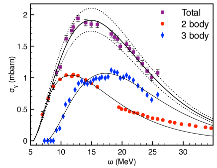
Figure 3: Parametrization of the ³He photodisintegration $(p,d)$ data from Refs. Ticcioni et al. (1973); Tornow et al. (2011) (red circles) and 3-body data from Ref. Faul et al. (1981) (blue rombs) are shown along with their sum (magenta squares) and the respective fits defined in Eqs. (50,51).

The structure functions are obtained according to

$$F_{1}^{\rm real}(\nu,Q^{2}) = \frac{M\omega}{4\pi^{2}\alpha}\sigma_{\gamma}^{\rm tot}(\omega)f_{1}^{\rm real}(Q^{2})$$

$$F_{2}^{\rm real}(\nu,Q^{2}) = \frac{\nu Q^{2}}{M\vec{q}\,^{2}}F_{1}^{\rm real}(\nu,Q^{2}).$$ (52)

A relation between $F_{1}$ and $F_{2}$ of this form is equivalent to a vanishing of the respective contribution to the longitudinal cross section. Above, $\omega=\nu-Q^{2}/2M$, and the function of $Q^{2}$ obtained from a fit to QE data is

$$f_{1}^{\rm real}(Q^{2}) = \frac{1+a_{3}\,Q^{2}}{(1+b_{3}\,Q^{4})^{c_{3}}},$$ (53)

with $a_{3}=167(6)$ GeV^-2, $b_{3}=94(16)$ GeV^-4 and $c_{3}=2.5(2)$.

The uncertainties of the parameters were obtained in the following way. At the first step, we fixed $f_{2}^{QE}=f_{1}^{QE}$ and $f_{2}^{real}=f_{1}^{real}$, and fitted 180^∘ data by Jones et al. Jones et al. (1979), 144.5^∘ data by Marchand et al. Marchand et al. (1985), 134.5^∘ data by Dow et al. Dow et al. (1988), as well as the transverse part of the L-T separated data by Retzlaff et al. Retzlaff et al. (1994). Because our fits were designed, in the first place, to provide a reliable input to the Lamb shift calculation where the integrals are weighted heavily towards low values of $Q^{2}$, we aimed at ensuring that we describe the data at lowest $Q^{2}$ values in the best possible way. In particular, the real photon data and the low-energy 180^∘ data by Jones et al. Jones et al. (1979) at $Q^{2}\approx 0.005$ GeV² and slightly above, fix the parameters $a_{1}$ and $a_{3}$, while they are not sensitive to other parameters. Fixing $a_{1,3}$ from a low-energy fit, we determined other parameters including other backward data. After the transverse part was determined, we turned to forward data at 36^∘ and 60^∘ by Marchand et al. Marchand et al. (1985) and 54^∘ data by Dow et al. Dow et al. (1988), as well as data on the longitudinal response function by Retzlaff et al. Retzlaff et al. (1994). While no further modification was necessary for $f_{2}^{real}$, an additional adjustment of $f_{2}^{QE}$ at low values of $Q^{2}$ was required. The fit via the function $f_{2}^{QE}$ is, however, only determined for $Q^{2}\geq Q_{min}^{2}\approx 0.009$ GeV², no data below that value are available at forward angles.

The behavior of $f_{2}^{QE}$ at lower virtualities, governed by the parameter $a_{2}$, is crucial for evaluating the Lamb shift. We proceeded as follows. Setting $a_{2}=0$ first, we obtained the reference value of the parameter $b_{2}=54.0(2.0)$ GeV^-2 from a fit at $Q^{2}\geq 0.02$ GeV², the value chosen to lie above $Q_{min}^{2}$. As the second step, we studied the extrapolation of $f_{2}^{QE}(a_{2}=0)$ to $0\leq Q^{2}\leq Q_{min}^{2}$ by means of a 3^rd order polynomial,

$$g(Q^{2},Q_{min}^{2})=\sum_{n=0}^{3}\frac{(Q^{2}-Q_{min}^{2})^{n}}{n!}g_{n}.$$ (54)

We fixed its value and first two derivatives at $Q^{2}=Q^{2}_{min}$, i.e. $g_{0,1,2}$ to those of the function $f_{2}^{QE}(a_{2}=0,Q^{2}=Q_{min}^{2})$ and treated $g_{3}$ as a free parameter with constraints:

$$|g_{3}|\leq 3\left|\left[f_{2}^{QE}(a_{2}=0,Q^{2}=Q_{min}^{2})\right]^{\prime\prime\prime}\right|,$$

$$g(Q^{2},Q_{min}^{2})\geq 0\;\;\;{\rm for}\;\;\;Q^{2}\geq 0,$$ (55)

the latter constraint being due to the fact that $F_{2}^{QE}$ is a cross section that is positive definite. This gives us the upper and lower value of $g(Q^{2},Q_{min}^{2})$ evaluated at $Q^{2}=0$ which we now identify with the parameter $a_{2}$. We also studied the dependence of choosing the matching point 0.009 GeV${}^{2}\leq Q_{min}^{2}\geq 0.017$ GeV², and obtained after averaging $a_{2}=0.014\pm 0.014$. The uncertainty is a combined systematical and statistical one, but it is dominated by the systematical uncertainty, the one due to the extrapolation. Statistical uncertainty obtained from that of the parameter $b_{2}$ which fixes $\left[f_{2}^{QE}(a_{2}=0,Q^{2}=Q_{min}^{2})\right]^{\prime\prime\prime}$ only contributes a couple percent.

Finally, we used parameter $a_{2}$ as fixed, and refit of $f_{2}^{QE}$, allowing once again the parameter $b_{2}$ to vary. The resulting value $b_{2}=(52.0\pm 2.0)$ GeV^-2 nicely agrees with the previously obtained $b_{2}=(54.0\pm 2.0)$ GeV^-2, which serves as an a posteriori test of validity of this procedure.

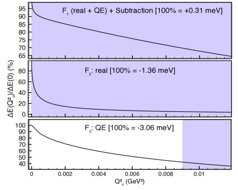
Figure 4: Saturation of the dispersion integrals for $\Delta E^{\rm subt}+\Delta E^{\rm inel}[F_{1}^{\rm QE}+F_{1}^{\rm real}]$ contribution (upper panel), $\Delta E^{\rm inel}[F_{2}^{\rm real}]$ (middle panel), $\Delta E^{\rm.inel}[F_{2}^{\rm QE}]$ (lower panel) as function of the lower limit of integration $Q_{0}^{2}$, in percent of the full result corresponding to $Q_{0}^{2}=0$. In each panel, the absolute value of each contribution to the Lamb shift in $\mu\,^{3}$He in meV is indicated. Shaded areas indicate the regions where experimental data are available.

To address the respective uncertainty for the Lamb shift calculation, we study the saturation of the dispersion integrals in Eqs. (II, 21), as function of the lower limit of the $Q^{2}$-integral, while the integral over energy is carried out over the full allowed range in the quasielastic region. In doing so, we consider the sum of the subtraction term and the inelastic contribution due to $F_{1}$, and separately contributions of $F_{2}^{\rm real}$ and $F_{2}^{\rm QE}$ to Eq. (21) as function of the lower limit of integration $Q_{0}^{2}$ in the range $0\leq Q_{0}^{2}\leq Q_{\rm min}^{2}$and take the value of each of these integrals with $Q_{0}^{2}=0$ for 100%. Results are shown in Fig. 4. We observe that the sum $\Delta E^{\rm subt}+\Delta E^{{\rm inel},\,F_{1}}$ is not very sensitive to the details of the extrapolation below $Q_{\rm min}^{2}\approx 0.005$ GeV²: only about 20% of the total of that contribution to the Lamb shift comes from $Q_{0}^{2}\leq Q_{\rm min}^{2}$, which in absolute values is mere 0.06 meV.

Instead, both $F_{2}$ contributions are very sensitive to the lower limit of the integration: for $F_{2}^{\rm real}$ about 94% comes from $Q_{0}^{2}\leq Q_{\rm min}^{2}$, whereas for $F_{2}^{\rm QE}$ about 40% comes from that range. We recall that the former contribution is fixed at the extremes of the explored range, by real photon data at $Q^{2}=0$ and by the QE data at $Q^{2}=Q_{\rm min}^{2}$. We conclude that the uncertainty of $\Delta E^{\rm inel,\,real}$ is given by the uncertainties of the data. However, this is not the case for the QE contribution that is only fixed at $Q^{2}\geq Q_{\rm min}^{2}$. The fit to data above that value is consistent with the function $f_{2}^{QE}$ vanishing at $Q^{2}=0$, but it going to a finite small positive number instead is also not excluded. We expect the extrapolating function to be smooth because the point $Q_{\rm min}^{2}\approx 0.009$ GeV² corresponds roughly to a distance of 2 fm, on the exterior of the charge distribution of ³He that has a radius of 1.97 fm, so we expect no structure beyond this point.

It is seen that already a 5% measurement at largest angle in the considered range will reduce the uncertainty of the nuclear polarizability contribution by a factor of $\sim 2$, leaving the Zemach contribution the main source of the uncertainty in the full TPE calculation. Further improvement in the precision of the inelastic contribution will only have a marginal effect, unless a more precise determination of the 3^rd Zemach moment from elastic $e-\,^{3}$He scattering data will become possible.

References

- Antognini et al. (2011) A. Antognini, F. Nez, F. D. Amaro, F. Biraben, J. M. R. Cardoso, D. S. Covita, A. Dax, S. Dhawan, L. M. P. Fernandes, A. Giesen, et al., Can. J. Phys. 89, 47 (2011).
- Pohl et al. (2010) R. Pohl et al., Nature 466, 213 (2010).
- Antognini et al. (2013a) A. Antognini et al., Science 339, 417 (2013a).
- Pohl et al. (2013) R. Pohl, R. Gilman, G. A. Miller, and K. Pachucki, Ann. Rev. Nucl. Part. Sci. 63, 175 (2013), eprint 1301.0905.
- Carlson (2015) C. E. Carlson, Prog. Part. Nucl. Phys. 82, 59 (2015), eprint 1502.05314.
- Pohl et al. (2016) R. Pohl, F. Nez, L. M. P. Fernandes, F. D. Amaro, F. Biraben, J. M. R. Cardoso, D. S. Covita, A. Dax, S. Dhawan, M. Diepold, et al., Science 353, 669 (2016).
- Antognini et al. (2016) A. Antognini et al., EPJ Web Conf. 113, 01006 (2016), eprint 1509.03235.
- Borie (2012) E. Borie, Annals Phys. 327, 733 (2012).
- Antognini et al. (2013b) A. Antognini, F. Kottmann, F. Biraben, P. Indelicato, F. Nez, and R. Pohl, Annals Phys. 331, 127 (2013b), eprint 1208.2637.
- Karplus et al. (1952) R. Karplus, A. Klein, and J. Schwinger, Phys. Rev. 86, 288 (1952).
- Eides et al. (2001) M. I. Eides, H. Grotch, and V. A. Shelyuto, Phys. Rept. 342, 63 (2001), eprint hep-ph/0002158.
- Sick (2014) I. Sick, Phys. Rev. C90, 064002 (2014), eprint 1412.2603.
- Shiner et al. (1995) D. Shiner, R. Dixson, and V. Vedantham, Phys. Rev. Lett. 74, 3553 (1995).
- Cancio Pastor et al. (2012) P. Cancio Pastor, L. Consolino, G. Giusfredi, P. De Natale, M. Inguscio, V. A. Yerokhin, and K. Pachucki, Physical Review Letters 108, 143001 (2012), eprint 1201.1362.
- Pachucki et al. (2012) K. Pachucki, V. A. Yerokhin, and P. Cancio Pastor, Phys. Rev. A 85, 042517 (2012), eprint 1203.6840.
- van Rooij et al. (2011) R. van Rooij, J. S. Borbely, J. Simonet, M. D. Hoogerland, K. S. E. Eikema, R. A. Rozendaal, and W. Vassen, Science 333, 196 (2011), eprint 1105.4974.
- Tucker-Smith and Yavin (2011) D. Tucker-Smith and I. Yavin, Phys. Rev. D83, 101702 (2011), eprint 1011.4922.
- Batell et al. (2011) B. Batell, D. McKeen, and M. Pospelov, Phys. Rev. Lett. 107, 011803 (2011), eprint 1103.0721.
- Carlson and Rislow (2012) C. E. Carlson and B. C. Rislow, Phys. Rev. D86, 035013 (2012), eprint 1206.3587.
- Liu et al. (2016) Y.-S. Liu, D. McKeen, and G. A. Miller, Phys. Rev. Lett. 117, 101801 (2016), eprint 1605.04612.
- Nevo Dinur et al. (2016) N. Nevo Dinur, C. Ji, S. Bacca, and N. Barnea, Phys. Lett. B755, 380 (2016), eprint 1512.05773.
- Hernandez et al. (2016) O. J. Hernandez, N. Nevo Dinur, C. Ji, S. Bacca, and N. Barnea, Hyperfine Interact. 237, 158 (2016), eprint 1604.06496.
- Pachucki (1999) K. Pachucki, Phys. Rev. A60, 3593 (1999).
- Martynenko (2006) A. P. Martynenko, Phys. Atom. Nucl. 69, 1309 (2006), eprint hep-ph/0509236.
- Carlson and Vanderhaeghen (2011) C. E. Carlson and M. Vanderhaeghen, Phys. Rev. A84, 020102 (2011), eprint 1101.5965.
- Birse and McGovern (2012) M. C. Birse and J. A. McGovern, Eur. Phys. J. A48, 120 (2012), eprint 1206.3030.
- Gorchtein et al. (2013) M. Gorchtein, F. J. Llanes-Estrada, and A. P. Szczepaniak, Phys. Rev. A87, 052501 (2013), eprint 1302.2807.
- Carlson et al. (2014) C. E. Carlson, M. Gorchtein, and M. Vanderhaeghen, Phys. Rev. A89, 022504 (2014), eprint 1311.6512.
- Nevado and Pineda (2008) D. Nevado and A. Pineda, Phys. Rev. C77, 035202 (2008), eprint 0712.1294.
- Alarcon et al. (2014) J. M. Alarcon, V. Lensky, and V. Pascalutsa, Eur. Phys. J. C74, 2852 (2014), eprint 1312.1219.
- Peset and Pineda (2015) C. Peset and A. Pineda, Eur. Phys. J. A51, 156 (2015), eprint 1508.01948.
- Pachucki (2011) K. Pachucki, Phys. Rev. Lett. 106, 193007 (2011), eprint 1102.3296.
- Friar (2013) J. L. Friar, Phys. Rev. C88, 034003 (2013), eprint 1306.3269.
- Hernandez et al. (2014) O. J. Hernandez, C. Ji, S. Bacca, N. Nevo Dinur, and N. Barnea, Phys. Lett. B736, 344 (2014), eprint 1406.5230.
- Pachucki and Wienczek (2015) K. Pachucki and A. Wienczek, Phys. Rev. A91, 040503 (2015), eprint 1501.07451.
- Krauth et al. (2016) J. J. Krauth, M. Diepold, B. Franke, A. Antognini, F. Kottmann, and R. Pohl, Annals Phys. 366, 168 (2016), eprint 1506.01298.
- Amroun et al. (1994) A. Amroun et al., Nucl. Phys. A579, 596 (1994).
- Sick (2008) I. Sick, Phys. Rev. C77, 041302 (2008).
- Krutov et al. (2015) A. A. Krutov, A. P. Martynenko, G. A. Martynenko, and R. N. Faustov, J. Exp. Theor. Phys. 120, 73 (2015), [Zh. Eksp. Teor. Fiz.147,no.1,85(2015)].
- De Vries et al. (1987) H. De Vries, C. W. De Jager, and C. De Vries, Atom. Data Nucl. Data Tabl. 36, 495 (1987).
- Benhar et al. (2006) O. Benhar, D. Day, and I. Sick (2006), eprint nucl-ex/0603032.
- Benhar et al. (2008) O. Benhar, D. day, and I. Sick, Rev. Mod. Phys. 80, 189 (2008), eprint nucl-ex/0603029.
- Jones et al. (1979) E. C. Jones, W. L. Bendel, L. W. Fagg, and R. A. Lindgren, Phys. Rev. C19, 610 (1979).
- Chertok et al. (1969) B. T. Chertok, E. C. Jones, W. L. Bendel, and L. W. Fagg, Phys. Rev. Lett. 23, 34 (1969).
- Maieron et al. (2002) C. Maieron, T. W. Donnelly, and I. Sick, Phys. Rev. C65, 025502 (2002), eprint nucl-th/0109032.
- Bosted and Mamyan (2012) P. E. Bosted and V. Mamyan (2012), eprint 1203.2262.
- Bodek et al. (2014) A. Bodek, M. E. Christy, and B. Coopersmith, Eur. Phys. J. C74, 3091 (2014), eprint 1405.0583.
- Marchand et al. (1985) C. Marchand et al., Phys. Lett. B153, 29 (1985).
- Dow et al. (1988) K. Dow et al., Phys. Rev. Lett. 61, 1706 (1988).
- Bosted and Christy (2008) P. E. Bosted and M. E. Christy, Phys. Rev. C77, 065206 (2008), eprint 0711.0159.
- Christy and Bosted (2010) M. E. Christy and P. E. Bosted, Phys. Rev. C81, 055213 (2010), eprint 0712.3731.
- Gorchtein (2015) M. Gorchtein, Phys. Rev. Lett. 115, 222503 (2015), eprint 1508.02509.
- Levinger and Bethe (1950) J. S. Levinger and H. A. Bethe, Phys. Rev. 78, 115 (1950).
- Olive et al. (2014) K. A. Olive et al. (Particle Data Group), Chin. Phys. C38, 090001 (2014).
- Hagelstein et al. (2016) F. Hagelstein, R. Miskimen, and V. Pascalutsa, Prog. Part. Nucl. Phys. 88, 29 (2016), eprint 1512.03765.
- Chang et al. (2015) E. Chang, W. Detmold, K. Orginos, A. Parreno, M. J. Savage, B. C. Tiburzi, and S. R. Beane (NPLQCD), Phys. Rev. D92, 114502 (2015), eprint 1506.05518.
- Friar and Payne (1997) J. L. Friar and G. L. Payne, Phys. Rev. C56, 619 (1997), eprint nucl-th/9704032.
- Chen et al. (1998) J.-W. Chen, H. W. Griesshammer, M. J. Savage, and R. P. Springer, Nucl. Phys. A644, 221 (1998), eprint nucl-th/9806080.
- Retzlaff et al. (1994) G. A. Retzlaff et al., Phys. Rev. C49, 1263 (1994).
- Faul et al. (1981) D. D. Faul, B. L. Berman, P. Meyer, and D. L. Olson, Phys. Rev. C24, 849 (1981).
- Ticcioni et al. (1973) G. Ticcioni, S. N. Gardiner, J. L. Matthews, and R. O. Owens, Phys. Lett. B46, 369 (1973).
- Tornow et al. (2011) W. Tornow et al., Phys. Lett. B702, 121 (2011).