A dual consistent finite difference method with
narrow stencil second derivative operators

Abstract

We study the numerical solutions of time-dependent systems of partial differential equations, focusing on the implementation of boundary conditions. The numerical method considered is a finite difference scheme constructed by high order summation by parts operators, combined with a boundary procedure using penalties (SBP-SAT).

Recently it was shown that SBP-SAT finite difference methods can yield superconvergent functional output if the boundary conditions are imposed such that the discretization is dual consistent. We generalize these results so that they include a broader range of boundary conditions and penalty parameters. The results are also generalized to hold for narrow-stencil second derivative operators. The derivations are supported by numerical experiments.

Keywords: Finite differences, summation by parts, simultaneous approximation term, dual consistency, superconvergence, functionals, narrow stencil

1 Introduction

In this paper we consider a summation by parts (SBP) finite difference method, which is combined with a penalty technique denoted simultaneous approximation term (SAT) for the boundary conditions. The main advantages of the SBP-SAT finite difference methods are high accuracy, computational efficiency and provable stability. For a background on the history and the newer developments of SBP-SAT, see [19, 6].

A discrete differential operator $D_{1}$ is said to be a SBP-operator if it can be factorized by the inverse of a positive definite matrix $H$ and a difference operator $Q$, as specified later in equation (19). When $H$ is diagonal, $D_{1}$ consists of a $2p$-order accurate central difference approximation in the interior, but at the boundaries, the accuracy is limited to $p$th order. The global accuracy of the numerical solution can then be shown to be $p+1$, see [19, 18].

In many applications functionals are of interest, sometimes they are even more important than the primary solution itself (one example is lift or drag coefficients in computational fluid dynamics). It could be expected that functionals computed from the numerical solution would have the same order of accuracy as the solution itself. However, recently Hicken and Zingg [9] showed that when computing the numerical solution in a dual consistent way, the order of accuracy of the output functional is higher than the FD solution itself, in fact, the full $2p$ accuracy can be recovered. Related papers are [10, 8] which includes interesting work on SBP operators as quadrature rules and error estimators for functional errors. Note that this kind of superconvergent behavior was already known for example for finite element and discontinuous Galerkin methods, but it had not been proven for finite difference schemes before, see [9]. Later Berg and Nordström [1, 2, 3] showed that the results hold also for time-dependent problems.

In [9, 8] and [1] boundary conditions of Dirichlet type are considered (in [9] Neumann boundary conditions are included but are rewritten on first order form), and in [2, 3] boundary conditions of far-field type are derived. In this paper, we generalize these results by deriving penalty parameters that yield dual consistency for all energy stable boundary conditions of Robin type (including the special cases Dirichlet and Neumann). In contrast to [2, 3], where the boundary conditions were adapted to get the penalty in a certain form, we adapt the penalty after the boundary conditions instead. Furthermore, we extend the results such that they hold also for narrow-stencil second derivative operators (sometimes also denoted compact second derivative operators), where the term narrow is used to define explicit finite difference schemes with a minimal stencil width. In fact, the results even carry over to narrow-stencil second derivatives operators for variable coefficients (of the type considered for example in [12]).

To keep things simple we consider linear problems in one spatial dimension, however, note that this is not due to a limitation of the method. In [9, 8] the extension to higher dimensions, curvilinear grids and non-linear problems are discussed and implemented for stationary problems and in [3] the theory is applied to the time-dependent Navier–Stokes and Euler equations in two dimensions.

The paper is organized as follows: In Section 2 we consider hyperbolic systems of partial differential equations and derive a family of SAT parameters which guarantees a stable and dual consistent discretization. Since higher order differential equations can always be rewritten as first order systems, this result directly leads to penalty parameters for parabolic problems, when using wide-stencil second derivative operators. Next, these parameters are generalized such that they hold also for narrow-stencil second derivative operators. This is all done in Section 3. In Section 4 a special aspect of the stability for the narrow operators is discussed. The derivations are then followed by examples and numerical simulations in Section 5 and a summary is given in Section 6.

1.1 Preliminaries

We consider time-dependent partial differential equations (PDE) as

$$\begin{split}\hskip 1.0pt\mathcal{U}_{t}+\mathcal{L}(\hskip 1.0pt\mathcal{U})&=\mathcal{F},\hskip 20.0ptt\in[0,T],\hskip 20.0ptx\in\Omega,\end{split}$$ (1)

where $\mathcal{L}$ represents a linear, spatial differential operator and $\mathcal{F}(x,t)$ is a forcing function. For simplicity, we will assume that the sought solution $\hskip 1.0pt\mathcal{U}(x,t)$ satisfies homogeneous initial and boundary conditions. To derive the dual equations we follow [9, 1, 2] and pose the problem in a variational framework: Given a functional $\mathcal{J}(\hskip 1.0pt\mathcal{U})=\langle{\mathcal{G},\hskip 1.0pt\mathcal{U}}\rangle$, where $\mathcal{G}(x,t)$ is smooth weight function and where $\langle{\mathcal{G},\hskip 1.0pt\mathcal{U}}\rangle=\int_{\Omega}\mathcal{G}^{T}\hskip 1.0pt\mathcal{U}\,\mathrm{d}x$ refers to the standard $L^{2}$ inner product, we seek a function $\mathcal{V}(x,t)$ such that $\mathcal{J}(\hskip 1.0pt\mathcal{U})=\mathcal{J}^{*}(\mathcal{V})=\langle{\mathcal{V},\mathcal{F}}\rangle$. This defines the dual problem as

$$\begin{split}\mathcal{V}_{\tau}+\mathcal{L}^{*}(\mathcal{V})&=\mathcal{G},\hskip 20.0pt\tau\in[0,T],\hskip 20.0ptx\in\Omega,\end{split}$$ (2)

where $\mathcal{L}^{*}$ is the adjoint operator, given by $\langle{\mathcal{V},\mathcal{L}\hskip 1.0pt\mathcal{U}}\rangle=\langle{\mathcal{L}^{*}\mathcal{V},\hskip 1.0pt\mathcal{U}}\rangle$, and where $\mathcal{V}$ also satisfies homogeneous initial and boundary conditions. Note that the dual problem actually goes ”backward” in time; the expression in (2) is obtained using the transformation $\tau=T-t$.

Let $U$ and $V$ be discrete vectors approximating $\hskip 1.0pt\mathcal{U}$ and $\mathcal{V}$, respectively, and let $F$ and $G$ be projections of $\mathcal{F}$ and $\mathcal{G}$ onto a spatial grid. We discretize (1) using a stable and consistent SBP-SAT scheme, leading to

$$\begin{split}U_{t}+LU&=F,\hskip 20.0ptt\in[0,T].\end{split}$$ (3)

The SBP scheme has an associated matrix $H$ which defines a discrete inner product, as $\langle{G,U}\rangle_{{}_{H}}=G^{T}HU$ (when $\hskip 1.0pt\mathcal{U}$ is vector-valued, $H$ must be replaced by $\hskip 2.0pt\overline{H}$, which is defined later in the paper). Now the discrete adjoint operator is given by $L^{*}=H^{-1}L^{T}H$, since this leads to $\langle{V,LU}\rangle_{{}_{H}}=\langle{L^{*}V,U}\rangle_{{}_{H}}$ which mimics the continuous relation above.

If $L^{*}$ happens to be a consistent approximation of $\mathcal{L}^{*}$, then the discretization (3) is said to be dual consistent (if considering the stationary case) or spatially dual consistent, see [9, 1] respectively. When (3) is a stable and dual consistent discretization of (1), then the linear functional $J(U)=\langle{G,U}\rangle_{{}_{H}}$ is a $2p$-order accurate approximation of $\mathcal{J}(\hskip 1.0pt\mathcal{U})$, that is $J(U)=\mathcal{J}(\hskip 1.0pt\mathcal{U})+\mathcal{O}(h^{2p})$, and we thus have superconvergent functional output. To obtain such high accuracy it is necessary with compatible and sufficiently smooth data, see [9] for more details.

2 Hyperbolic systems

We start by considering a hyperbolic system of PDEs of reaction-advection type, namely

$$\begin{array}[]{rll}\hskip 1.0pt\mathcal{U}_{t}+\mathcal{R}\hskip 0.5pt\hskip 1.0pt\mathcal{U}+\mathcal{A}\hskip 0.5pt\hskip 1.0pt\mathcal{U}_{x}=&\mathcal{F},&x\in[x_{\scalebox{0.6}{$L$\hskip 1.0pt}},x_{\scalebox{0.6}{$R$\hskip 1.0pt}}],\vspace{4pt}\\ \mathcal{B}_{\scalebox{0.7}{$L$\hskip 1.0pt}}\hskip 1.0pt\mathcal{U}=&g_{\scalebox{0.6}{$L$\hskip 1.0pt}},&x=x_{\scalebox{0.6}{$L$\hskip 1.0pt}},\vspace{4pt}\\ \mathcal{B}_{\scalebox{0.7}{$R$\hskip 1.0pt}}\hskip 1.0pt\mathcal{U}=&g_{\scalebox{0.6}{$R$\hskip 1.0pt}},&x=x_{\scalebox{0.6}{$R$\hskip 1.0pt}},\end{array}$$ (7)

valid for $t\geq 0$ and augmented with initial data $\hskip 1.0pt\mathcal{U}(x,0)=\hskip 1.0pt\mathcal{U}_{0}(x)$. We let $\mathcal{R}\hskip 0.5pt$ and $\mathcal{A}\hskip 0.5pt$ be real-valued, symmetric $n\times n$ matrices. Further, $\mathcal{R}\hskip 0.5pt$ is positive semi-definite, that is $\mathcal{R}\hskip 0.5pt\geq 0$. The operators $\mathcal{B}_{\scalebox{0.7}{$L$\hskip 1.0pt}}$ and $\mathcal{B}_{\scalebox{0.7}{$R$\hskip 1.0pt}}$ define the form of the boundary conditions and their properties are specified in (16) below. The forcing function $\mathcal{F}(x,t)$, the initial data $\hskip 1.0pt\mathcal{U}_{0}(x)$ and the boundary data $g_{\scalebox{0.6}{$L$\hskip 1.0pt}}(t)$ and $g_{\scalebox{0.6}{$R$\hskip 1.0pt}}(t)$ are assumed to be compatible and sufficiently smooth such that the solution $\hskip 1.0pt\mathcal{U}(x,t)$ exists. We will refer to (7) as our primal problem.

2.1 Well-posedness using the energy method

We call (7) well-posed if it has a unique solution and is stable. Existence is guaranteed by using the right number of boundary conditions, and uniqueness then follows from the stability, [15, 7]. Next we show stability, using the energy method.

The PDE in the first row of (7) is multiplied by $\hskip 1.0pt\mathcal{U}^{T}$ from the left and integrated over the domain $\Omega=[x_{\scalebox{0.6}{$L$\hskip 1.0pt}},x_{\scalebox{0.6}{$R$\hskip 1.0pt}}]$. Using integration by parts we obtain

$$\frac{\mathrm{d}}{\mathrm{d}t}\|\hskip 1.0pt\mathcal{U}\|^{2}+2\langle{\hskip 1.0pt\mathcal{U},\mathcal{R}\hskip 0.5pt\hskip 1.0pt\mathcal{U}}\rangle =2\langle{\hskip 1.0pt\mathcal{U},\mathcal{F}}\rangle+\text{\text{BT}}_{L}+\text{\text{BT}}_{R}$$ (8)

where $\|\hskip 1.0pt\mathcal{U}\|^{2}=\langle{\hskip 1.0pt\mathcal{U},\hskip 1.0pt\mathcal{U}}\rangle=\int_{x_{\scalebox{0.6}{$L$\hskip 1.0pt}}}^{x_{\scalebox{0.6}{$R$\hskip 1.0pt}}}\hskip 1.0pt\mathcal{U}^{T}\hskip 1.0pt\mathcal{U}\,\mathrm{d}x$ and where

$$\text{\text{BT}}_{L}=\left.\hskip 1.0pt\mathcal{U}^{T}\mathcal{A}\hskip 0.5pt\hskip 1.0pt\mathcal{U}\right|_{x_{\scalebox{0.6}{$L$\hskip 1.0pt}}}, \text{\text{BT}}_{R}=-\left.\hskip 1.0pt\mathcal{U}^{T}\mathcal{A}\hskip 0.5pt\hskip 1.0pt\mathcal{U}\right|_{x_{\scalebox{0.6}{$R$\hskip 1.0pt}}}.$$

To bound the growth of the solution, we must ensure that the boundary conditions make $\text{\text{BT}}_{L}$ and $\text{\text{BT}}_{R}$ non-positive for zero data. We consider the matrix $\mathcal{A}\hskip 0.5pt$ above and assume that we have found a factorization such that

$$\mathcal{A}\hskip 0.5pt=Z\Delta Z^{T}, \Delta=\left[\begin{array}[]{ccc}\Delta_{+}\\ &\Delta_{0}\\ &&\Delta_{-}\end{array}\right], Z=\left[Z_{+},Z_{0},Z_{-}\right],$$ (12)

where $Z$ is non-singular. The parts of $\Delta$ are arranged such that $\Delta_{+}>0$, $\Delta_{0}=0$ and $\Delta_{-}<0$. According to Sylvester’s law of inertia, the matrices $\mathcal{A}\hskip 0.5pt$ and $\Delta$ have the same number of positive ($n_{+}$), negative ($n_{-}$) and zero ($n_{0}$) eigenvalues (for a non-singular $Z$), where $n=n_{+}+n_{0}+n_{-}$. To bound the terms $\text{\text{BT}}_{L}$ and $\text{\text{BT}}_{R}$, we have to give $n_{+}$ boundary conditions at $x=x_{\scalebox{0.6}{$L$\hskip 1.0pt}}$ and $n_{-}$ boundary conditions at $x=x_{\scalebox{0.6}{$R$\hskip 1.0pt}}$. We note that

$$\mathcal{A}\hskip 0.5pt=Z_{+}\Delta_{+}Z_{+}^{T}+Z_{-}\Delta_{-}Z_{-}^{T},$$ (13)

which gives

$$\text{\text{BT}}_{L}=\left.\hskip 1.0pt\mathcal{U}^{T}\left(Z_{+}\Delta_{+}Z_{+}^{T}+Z_{-}\Delta_{-}Z_{-}^{T}\right)\hskip 1.0pt\mathcal{U}\right|_{x_{\scalebox{0.6}{$L$\hskip 1.0pt}}}, \text{BT}_{R}=-\left.\hskip 1.0pt\mathcal{U}^{T}\left(Z_{+}\Delta_{+}Z_{+}^{T}+Z_{-}\Delta_{-}Z_{-}^{T}\right)\hskip 1.0pt\mathcal{U}\right|_{x_{\scalebox{0.6}{$R$\hskip 1.0pt}}}$$

where $Z_{+}^{T}\hskip 1.0pt\mathcal{U}$ represents the right-going variables (ingoing at the left boundary), and $Z_{-}^{T}\hskip 1.0pt\mathcal{U}$ represents the left-going variables (ingoing at the right boundary). The ingoing variables are given data in terms of known functions and outgoing variables, as

$$\left.Z_{+}^{T}\hskip 1.0pt\mathcal{U}\right|_{x_{\scalebox{0.6}{$L$\hskip 1.0pt}}}=\left.\widetilde{g}_{L}-R_{L}Z_{-}^{T}\hskip 1.0pt\mathcal{U}\right|_{x_{\scalebox{0.6}{$L$\hskip 1.0pt}}}, \left.Z_{-}^{T}\hskip 1.0pt\mathcal{U}\right|_{x_{\scalebox{0.6}{$R$\hskip 1.0pt}}}=\left.\widetilde{g}_{R}-R_{R}Z_{+}^{T}\hskip 1.0pt\mathcal{U}\right|_{x_{\scalebox{0.6}{$R$\hskip 1.0pt}}},$$ (14)

where $\widetilde{g}_{L}$, $\widetilde{g}_{R}$ are the known data and where the matrices $R_{L}$ and $R_{R}$ must be sufficiently small. Using the boundary conditions in (14), the boundary terms $\text{BT}_{L}$ and $\text{BT}_{R}$ become

$$\begin{split}\text{BT}_{L}&=\hskip 10.0pt\left.\hskip 1.0pt\mathcal{U}^{T}Z_{-}\left(\Delta_{-}+R_{L}^{T}\Delta_{+}R_{L}\right)Z_{-}^{T}\hskip 1.0pt\mathcal{U}\right|_{x_{\scalebox{0.6}{$L$\hskip 1.0pt}}}\hskip 2.0pt-\left.2\widetilde{g}_{L}^{T}\Delta_{+}R_{L}Z_{-}^{T}\hskip 1.0pt\mathcal{U}\right|_{x_{\scalebox{0.6}{$L$\hskip 1.0pt}}}\hskip 2.0pt+\widetilde{g}_{L}^{T}\Delta_{+}\widetilde{g}_{L}\\ \text{BT}_{R}&=-\left.\hskip 1.0pt\mathcal{U}^{T}Z_{+}\left(\Delta_{+}+R_{R}^{T}\Delta_{-}R_{R}\right)Z_{+}^{T}\hskip 1.0pt\mathcal{U}\right|_{x_{\scalebox{0.6}{$R$\hskip 1.0pt}}}+\left.2\widetilde{g}_{R}^{T}\Delta_{-}R_{R}Z_{+}^{T}\hskip 1.0pt\mathcal{U}\right|_{x_{\scalebox{0.6}{$R$\hskip 1.0pt}}}-\widetilde{g}_{R}^{T}\Delta_{-}\widetilde{g}_{R}.\end{split}$$ (15)

We define

$$\mathcal{C}_{L}=\Delta_{-}+R_{L}^{T}\Delta_{+}R_{L}, \mathcal{C}_{R}=-\Delta_{+}-R_{R}^{T}\Delta_{-}R_{R}$$

and note that if $\mathcal{C}_{L}$, $\mathcal{C}_{R}\leq 0$, the boundary terms in (15) will be non-positive for zero data. By integrating (8) in time we can now obtain a bound on $\|\hskip 1.0pt\mathcal{U}\|^{2}$. With boundary conditions on the form (14), we also know that the correct number of boundary conditions are specified at each boundary, which yields existence. Our problem is thus well-posed.

To relate the original boundary conditions in (7) to the ones in (14), we let

$$\mathcal{B}_{\scalebox{0.7}{$L$\hskip 1.0pt}}=P_{L}(Z_{+}^{T}+R_{L}Z_{-}^{T}),\hskip 30.0pt\mathcal{B}_{\scalebox{0.7}{$R$\hskip 1.0pt}}=P_{R}(Z_{-}^{T}+R_{R}Z_{+}^{T}),$$ (16)

where $P_{L}$ and $P_{R}$ are invertible scaling and/or permutation matrices. The data in (14) is identified as $\widetilde{g}_{L}=P_{L}^{-1}g_{\scalebox{0.6}{$L$\hskip 1.0pt}}$ and $\widetilde{g}_{R}=P_{R}^{-1}g_{\scalebox{0.6}{$R$\hskip 1.0pt}}$. We assume that the boundary conditions in (7) are properly chosen such that $R_{L}$ and $R_{R}$ are sufficiently small and hence $\mathcal{C}_{L}$, $\mathcal{C}_{R}\leq 0$.

Remark 2.1.

Note that the energy method is a sufficient but not necessary condition for stability and that it is rather restrictive with respect to the admissible boundary conditions. By rescaling the problem we could allow $R_{L}$ and $R_{R}$ to be larger, see [11, 7]. We will not consider this complication but simply require that $\mathcal{C}_{L}\leq 0$, $\mathcal{C}_{R}\leq 0$.

Remark 2.2.

In the homogeneous case, with boundary conditions such that $\mathcal{C}_{L}$, $\mathcal{C}_{R}\leq 0$, the growth rate in (8) becomes $\frac{\mathrm{d}}{\mathrm{d}t}\|\hskip 1.0pt\mathcal{U}\|^{2}\leq 0$. Integrating this in time we obtain the energy estimate $\|\hskip 1.0pt\mathcal{U}\|^{2}\leq\|\hskip 1.0pt\mathcal{U}_{0}\|^{2}$ and (7) is well-posed. Since (7) is an one-dimensional hyperbolic problem it is also possible to show strong well-posedness, i.e. that $\|\hskip 1.0pt\mathcal{U}\|$ is bounded by the data $g_{\scalebox{0.6}{$L$\hskip 1.0pt}}$, $g_{\scalebox{0.6}{$R$\hskip 1.0pt}}$, $\mathcal{F}$ and $\hskip 1.0pt\mathcal{U}_{0}$. See [11, 7] for different definitions of well-posedness.

2.2 The semi-discrete problem

We discretize in space using $N+1$ equidistant grid points $x_{i}=x_{\scalebox{0.6}{$L$\hskip 1.0pt}}+hi$, where $h=(x_{\scalebox{0.6}{$R$\hskip 1.0pt}}-x_{\scalebox{0.6}{$L$\hskip 1.0pt}})/N$ and $i=0,1,\ldots,N$. The semi-discrete scheme approximating (7) is written

$$\begin{split}U_{t}+(I_{N}\otimes\mathcal{R}\hskip 0.5pt)U+(D_{1}\otimes\mathcal{A}\hskip 0.5pt)U=F&+(H^{-1}e_{\hskip 1.0pt0\hskip 0.5pt}\otimes\Sigma_{0})(\mathcal{B}_{\scalebox{0.7}{$L$\hskip 1.0pt}}{U}_{\hskip 1.0pt0\hskip 0.5pt}-g_{\scalebox{0.6}{$L$\hskip 1.0pt}})\\ &+(H^{-1}e_{N}\otimes\Sigma_{N})(\mathcal{B}_{\scalebox{0.7}{$R$\hskip 1.0pt}}{U}_{N}-g_{\scalebox{0.6}{$R$\hskip 1.0pt}}),\end{split}$$ (17)

where $U=[U_{0}^{T},U_{1}^{T},\ldots,U_{N}^{T}]^{T}$ is a vector of length $n(N+1)$, such that $U_{i}(t)\approx\hskip 1.0pt\mathcal{U}(x_{i},t)$, and where $F_{i}(t)=\mathcal{F}(x_{i},t)$. The symbol $\otimes$ refers to the Kronecker product. The finite difference operator $D_{1}$ approximates $\partial/\partial x$ and satisfies the SBP-properties

$$\begin{array}[]{lclcl}\vspace{4pt}D_{1}=H^{-1}Q,&&\hskip 5.5ptH=H^{T}>0,&&Q+Q^{T}=E_{N}-E_{0}\\ \end{array}$$ (19)

where $E_{0}=e_{0}e_{0}^{T}$, $E_{N}=e_{N}e_{N}^{T}$ and $e_{0}=[1,0,\ldots,0]^{T}$ and $e_{N}=[0,\ldots,0,1]^{T}$. Note that $U_{0}=(e_{0}^{T}\otimes I_{n})U$ and $U_{N}=(e_{N}^{T}\otimes I_{n})U$. By $I_{N}$ and $I_{n}$ we refer to identity matrices of size $N+1$ and $n$, respectively. The boundary conditions are imposed using the SAT technique which is a penalty method. The penalty parameters $\Sigma_{0}$ and $\Sigma_{N}$ in (17) are at this point unknown, but are derived in the next subsections and presented in Theorem 2.6.

In this paper, we require that $H$ is diagonal, and in this case $D_{1}$ consists of a $2p$-order accurate central difference approximation in the interior and one-sided, $p$-order accurate approximations at the boundaries. Examples of SBP operators can be found in [17, 13]. For more details about SBP-SAT, see [18] and references therein.

2.3 Numerical stability using the energy method

Just as in the continuous case we use the energy method to show stability. We multiply (17) by $U^{T}\hskip 2.0pt\overline{H}$ from the left, where $\hskip 2.0pt\overline{H}=H\otimes I_{n}$, and then add the transpose of the result. Thereafter using the SBP-properties in (19) we obtain

$$\frac{\mathrm{d}}{\mathrm{d}t}\|U\|^{2}_{{}_{H}}+2{U}^{T}(H\otimes\mathcal{R}\hskip 0.5pt){U} =2\langle{U,F}\rangle_{{}_{H}}+\text{BT}_{L}^{Disc.}+\text{BT}_{R}^{Disc.},$$

where $\|U\|^{2}_{{}_{H}}=\langle{U,U}\rangle_{{}_{H}}=U^{T}\hskip 2.0pt\overline{H}U$ is the discrete $L^{2}$-norm and where

$$\begin{split}\text{BT}_{L}^{Disc.}&=U_{\hskip 1.0pt0\hskip 0.5pt}^{T}\left(\hskip 9.0pt\mathcal{A}\hskip 0.5pt+\Sigma_{0}\hskip 2.0pt\mathcal{B}_{\scalebox{0.7}{$L$\hskip 1.0pt}}\hskip 1.0pt+\hskip 1.0pt\mathcal{B}_{\scalebox{0.7}{$L$\hskip 1.0pt}}^{T}\Sigma_{0}^{T}\hskip 3.0pt\right){U}_{\hskip 1.0pt0\hskip 0.5pt}\hskip 2.0pt-U_{\hskip 1.0pt0\hskip 0.5pt}^{T}\Sigma_{0}\hskip 2.0ptg_{\scalebox{0.6}{$L$\hskip 1.0pt}}\hskip 1.0pt-g_{\scalebox{0.6}{$L$\hskip 1.0pt}}^{T}\Sigma_{0}^{T}\hskip 2.0ptU_{\hskip 1.0pt0\hskip 0.5pt},\\ \text{BT}_{R}^{Disc.}&=U_{N}^{T}\left(-\mathcal{A}\hskip 0.5pt+\Sigma_{N}\mathcal{B}_{\scalebox{0.7}{$R$\hskip 1.0pt}}+\mathcal{B}_{\scalebox{0.7}{$R$\hskip 1.0pt}}^{T}\Sigma_{N}^{T}\right)U_{N}-U_{N}^{T}\Sigma_{N}g_{\scalebox{0.6}{$R$\hskip 1.0pt}}-g_{\scalebox{0.6}{$R$\hskip 1.0pt}}^{T}\Sigma_{N}^{T}U_{N}.\end{split}$$ (20)

We define $C_{0}=\mathcal{A}\hskip 0.5pt+\Sigma_{0}\mathcal{B}_{\scalebox{0.7}{$L$\hskip 1.0pt}}+\mathcal{B}_{\scalebox{0.7}{$L$\hskip 1.0pt}}^{T}\Sigma_{0}^{T}$ and $C_{N}=-\mathcal{A}\hskip 0.5pt+\Sigma_{N}\mathcal{B}_{\scalebox{0.7}{$R$\hskip 1.0pt}}+\mathcal{B}_{\scalebox{0.7}{$R$\hskip 1.0pt}}^{T}\Sigma_{N}^{T}$. For stability $\text{BT}_{L}^{Disc.}$ and $\text{BT}_{R}^{Disc.}$ must be non-positive for zero boundary data, i.e. $C_{0}\leq 0$ and $C_{N}\leq 0$. We make the following ansätze for the penalty parameters:

$$\Sigma_{0} =(Z_{+}\Pi_{0}+Z_{-}\Gamma_{0})P_{L}^{-1}, \Sigma_{N} =(Z_{+}\Gamma_{N}+Z_{-}\Pi_{N})P_{R}^{-1}.$$ (21)

Taking the left boundary as example and using (13), (16) and (21) we obtain

$$C_{0} =\left[\begin{array}[]{c}Z_{+}^{T}\\ Z_{-}^{T}\end{array}\right]^{T}\left[\begin{array}[]{cc}\Delta_{+}+\Pi_{0}+\Pi_{0}^{T}&\Pi_{0}R_{L}+\Gamma_{0}^{T}\\ \Gamma_{0}+R_{L}^{T}\Pi_{0}^{T}&\Delta_{-}+\Gamma_{0}R_{L}+R_{L}^{T}\Gamma_{0}^{T}\end{array}\right]\left[\begin{array}[]{c}Z_{+}^{T}\\ Z_{-}^{T}\end{array}\right].$$ (28)

2.4 The dual problem

Given the functional $\mathcal{J}(\hskip 1.0pt\mathcal{U})=\langle{\mathcal{G},\hskip 1.0pt\mathcal{U}}\rangle$, the dual problem of (7) is

$$\begin{array}[]{rll}\mathcal{V}_{\tau}+\mathcal{R}\hskip 0.5pt\mathcal{V}-\mathcal{A}\hskip 0.5pt\mathcal{V}_{x}=&\mathcal{G},&x\in[x_{\scalebox{0.6}{$L$\hskip 1.0pt}},x_{\scalebox{0.6}{$R$\hskip 1.0pt}}],\vspace{4pt}\\ \widetilde{\mathcal{B}_{\scalebox{0.7}{$L$\hskip 1.0pt}}}\mathcal{V}=&\widetilde{\hskip 1.0ptg_{\scalebox{0.6}{$L$\hskip 1.0pt}}},&x=x_{\scalebox{0.6}{$L$\hskip 1.0pt}},\vspace{4pt}\\ \widetilde{\mathcal{B}_{\scalebox{0.7}{$R$\hskip 1.0pt}}}\mathcal{V}=&\widetilde{g_{\scalebox{0.6}{$R$\hskip 1.0pt}}},&x=x_{\scalebox{0.6}{$R$\hskip 1.0pt}},\end{array}$$ (32)

which holds for $\tau\geq 0$ and is complemented with the initial condition $\mathcal{V}(x,0)=\mathcal{V}_{0}(x)$. The boundary operators in (32) have the form

$$\widetilde{\mathcal{B}_{\scalebox{0.7}{$L$\hskip 1.0pt}}}=\widetilde{P_{L}}(Z_{-}^{T}+\widetilde{R_{L}}Z_{+}^{T}), \widetilde{\mathcal{B}_{\scalebox{0.7}{$R$\hskip 1.0pt}}}=\widetilde{P_{R}}(Z_{+}^{T}+\widetilde{R_{R}}Z_{-}^{T}),$$ (33)

where $\widetilde{P_{L}}$ and $\widetilde{P_{R}}$ are arbitrary invertible matrices and $\widetilde{R_{L}}$ and $\widetilde{R_{R}}$ depend on the primal boundary conditions as

$$\widetilde{R_{L}}=-\Delta_{-}^{-1}R_{L}^{T}\Delta_{+}, \widetilde{R_{R}}=-\Delta_{+}^{-1}R_{R}^{T}\Delta_{-}.$$ (34)

The claim that (32), (33) and (34) describes the dual problem is motivated below: Using the notation in (1) and (2) we identify the spatial operators of (7) and (32) as

$$\mathcal{L}=\mathcal{R}\hskip 0.5pt+\mathcal{A}\hskip 0.5pt\frac{\partial}{\partial x}, \mathcal{L}^{*}=\mathcal{R}\hskip 0.5pt-\mathcal{A}\hskip 0.5pt\frac{\partial}{\partial x},$$ (35)

respectively. For (32) to be the dual problem of (7), $\mathcal{L}$ and $\mathcal{L}^{*}$ must fulfill the relation $\langle{\mathcal{V},\mathcal{L}\hskip 1.0pt\mathcal{U}}\rangle=\langle{\mathcal{L}^{*}\mathcal{V},\hskip 1.0pt\mathcal{U}}\rangle$. Using integration by parts we obtain

$$\langle{\mathcal{V},\mathcal{L}\hskip 1.0pt\mathcal{U}}\rangle =\langle{\mathcal{L}^{*}\mathcal{V},\hskip 1.0pt\mathcal{U}}\rangle+[\mathcal{V}^{T}\mathcal{A}\hskip 0.5pt\hskip 1.0pt\mathcal{U}]_{x_{\scalebox{0.6}{$L$\hskip 1.0pt}}}^{x_{\scalebox{0.6}{$R$\hskip 1.0pt}}}$$

and we see that $\mathcal{V}^{T}\mathcal{A}\hskip 0.5pt\hskip 1.0pt\mathcal{U}$ must be zero at both boundaries. (The boundary conditions for the dual problem are defined as the minimal set of homogeneous conditions such that all boundary terms vanish after that that the homogeneous boundary conditions for the primal problem have been applied, see [1].) Using the boundary conditions of the primal problem, (14), followed by the dual boundary conditions, (32), (33), yields (for zero data)

$$\left.\mathcal{V}^{T}\mathcal{A}\hskip 0.5pt\hskip 1.0pt\mathcal{U}\right|_{x_{\scalebox{0.6}{$L$\hskip 1.0pt}}} =\left.-\mathcal{V}^{T}Z_{+}\left(\Delta_{+}R_{L}+\widetilde{R_{L}}^{T}\Delta_{-}\right)Z_{-}^{T}\hskip 1.0pt\mathcal{U}\right|_{x_{\scalebox{0.6}{$L$\hskip 1.0pt}}}$$

$$\left.\mathcal{V}^{T}\mathcal{A}\hskip 0.5pt\hskip 1.0pt\mathcal{U}\right|_{x_{\scalebox{0.6}{$R$\hskip 1.0pt}}} =-\left.\mathcal{V}^{T}Z_{-}\left(\widetilde{R_{R}}^{T}\Delta_{+}+\Delta_{-}R_{R}\right)Z_{+}^{T}\hskip 1.0pt\mathcal{U}\right|_{x_{\scalebox{0.6}{$R$\hskip 1.0pt}}}$$

and if (34) holds, then $\mathcal{V}^{T}\mathcal{A}\hskip 0.5pt\hskip 1.0pt\mathcal{U}=0$ at both boundaries and the above claim is confirmed.

Remark 2.3.

A functional can also include outgoing solution terms from the boundary, as $\mathcal{J}(\hskip 1.0pt\mathcal{U})=\langle{\mathcal{G},\hskip 1.0pt\mathcal{U}}\rangle+\alpha\Delta_{+}Z_{+}^{T}\hskip 1.0pt\mathcal{U}|_{x_{\scalebox{0.6}{$R$\hskip 1.0pt}}}+\beta\Delta_{-}Z_{-}^{T}\hskip 1.0pt\mathcal{U}|_{x_{\scalebox{0.6}{$L$\hskip 1.0pt}}}$. This would specify the boundary data in (32) to $\widetilde{\hskip 1.0ptg_{\scalebox{0.6}{$L$\hskip 1.0pt}}}=-\widetilde{P_{L}}\beta^{T}$ and $\widetilde{g_{\scalebox{0.6}{$R$\hskip 1.0pt}}}=\widetilde{P_{R}}\alpha^{T}$, compare with [9]. For simplicity we consider $\mathcal{J}(\hskip 1.0pt\mathcal{U})=\langle{\mathcal{G},\hskip 1.0pt\mathcal{U}}\rangle$ which means that actually, the boundary data in (32) is zero.

2.4.1 Well-posedness of the dual problem

The growth rate for the dual problem is given by

$$\frac{d}{d\tau}\|\mathcal{V}\|^{2}+2\langle{\mathcal{V},\mathcal{R}\hskip 0.5pt\mathcal{V}}\rangle=\text{BT}_{L}^{dual}+\text{BT}_{R}^{dual}$$

where the boundary terms are (the homogeneous boundary conditions have been applied)

$$\text{BT}_{L}^{dual}=\mathcal{V}^{T}Z_{+}\widetilde{\mathcal{C}_{L}}\left.Z_{+}^{T}\mathcal{V}\right|_{x_{\scalebox{0.6}{$L$\hskip 1.0pt}}}, \text{BT}_{R}^{dual}=\mathcal{V}^{T}Z_{-}\widetilde{\mathcal{C}_{R}}\left.Z_{-}^{T}\mathcal{V}\right|_{x_{\scalebox{0.6}{$R$\hskip 1.0pt}}}$$

and where $\widetilde{\mathcal{C}_{L}}=-\Delta_{+}-\Delta_{+}R_{L}\Delta_{-}^{-1}R_{L}^{T}\Delta_{+}$ and $\widetilde{\mathcal{C}_{R}}=\Delta_{-}+\Delta_{-}R_{R}\Delta_{+}^{-1}R_{R}^{T}\Delta_{-}$. For well-posedness of the dual problem $\widetilde{\mathcal{C}_{L}}\leq 0$ and $\widetilde{\mathcal{C}_{R}}\leq 0$ are necessary.

Recall that the primal problem is well-posed if $\mathcal{C}_{L}$, $\mathcal{C}_{R}\leq 0$. The dual demand $\widetilde{\mathcal{C}_{L}}\leq 0$ is directly fulfilled if $\mathcal{C}_{L}\leq 0$ and $\widetilde{\mathcal{C}_{R}}\leq 0$ follows from $\mathcal{C}_{R}\leq 0$. (In the special case when $R_{L},R_{R}$ are square, invertible matrices, this is trivial. For general $R_{L},R_{R}$ it can be shown with the help of Sylvester’s determinant theorem.) We conclude that the dual problem (32) with (33), (34) is well-posed if the primal problem (7) with (16) is well-posed.

Remark 2.4.

In [2, 3] the dual consistent schemes are constructed by first designing the boundary conditions (for incompletely parabolic problems) such that both the primal and the dual problem are well-posed. Their different approach can partly be explained by their wish to have the boundary conditions in the special form $H_{L,R}U\mp BU_{x}=G_{L,R}$. Looking e.g. at Eq. (30) in [2], we note that after applying the boundary conditions, $U^{T}M_{L}U\geq 0$ is needed for stability. However, if $B$ is singular, replacing $BU_{x}$ by $\pm H_{L,R}U$ does not guarantee that all conditions have been completely used, and $u$ and $p$ in $U=[p,u]^{T}$ in $U^{T}M_{L}U$ can be linearly dependent. Therefore the demand $M_{L}\geq 0$ in (31) is unnecessarily strong and gives some extra restrictions on the boundary conditions.

2.4.2 Discretization of the dual problem

The semi-discrete scheme approximating the dual problem (32) is written

$$\begin{split}V_{\tau}+(I_{N}\otimes\mathcal{R}\hskip 0.5pt)V-(D_{1}\otimes\mathcal{A}\hskip 0.5pt)V=G&+(H^{-1}e_{0}\otimes\widetilde{\Sigma_{0}})(\widetilde{\mathcal{B}_{\scalebox{0.7}{$L$\hskip 1.0pt}}}{V}_{0}-\widetilde{\hskip 1.0ptg_{\scalebox{0.6}{$L$\hskip 1.0pt}}})\\ &+(H^{-1}e_{N}\otimes\widetilde{\Sigma_{N}})(\widetilde{\mathcal{B}_{\scalebox{0.7}{$R$\hskip 1.0pt}}}V_{N}-\widetilde{g_{\scalebox{0.6}{$R$\hskip 1.0pt}}}),\end{split}$$ (36)

where $V_{i}(\tau)$ represents $\mathcal{V}(x_{i},\tau)$. The SAT parameters $\widetilde{\Sigma_{0}}$ and $\widetilde{\Sigma_{N}}$ are yet unknown.

2.5 Dual consistency

The semi-discrete scheme (17) is rewritten as $U_{t}+LU=\text{RHS}$, where

$$L =(I_{N}\otimes\mathcal{R}\hskip 0.5pt)+(D_{1}\otimes\mathcal{A}\hskip 0.5pt)-(H^{-1}E_{0}\otimes\Sigma_{0}\mathcal{B}_{\scalebox{0.7}{$L$\hskip 1.0pt}})-(H^{-1}E_{N}\otimes\Sigma_{N}\mathcal{B}_{\scalebox{0.7}{$R$\hskip 1.0pt}})$$

and where RHS only depends on known data. In contrast to the continuous counterpart $\mathcal{L}$, $L$ includes the boundary conditions explicitly. According to [2], the discrete adjoint operator is given by $L^{*}=\hskip 2.0pt\overline{H}^{-1}L^{T}\hskip 2.0pt\overline{H}$, which, using (19), leads to

$$\begin{split}L^{*}&=(I_{N}\otimes\mathcal{R}\hskip 0.5pt)-(D_{1}\otimes\mathcal{A}\hskip 0.5pt)-(H^{-1}E_{0}\otimes\mathcal{B}_{\scalebox{0.7}{$L$\hskip 1.0pt}}^{T}\Sigma_{0}^{T}+\mathcal{A}\hskip 0.5pt)-(H^{-1}E_{N}\otimes\mathcal{B}_{\scalebox{0.7}{$R$\hskip 1.0pt}}^{T}\Sigma_{N}^{T}-\mathcal{A}\hskip 0.5pt)\end{split}$$ (37)

If $L^{*}$ is a consistent approximation of $\mathcal{L}^{*}$ in (35), then the scheme (17) is dual consistent. Looking at (36), we see that $L^{*}$ must have the form

$$(L^{*})^{goal} =(I_{N}\otimes\mathcal{R}\hskip 0.5pt)-(D_{1}\otimes\mathcal{A}\hskip 0.5pt)-(H^{-1}E_{0}\otimes\widetilde{\Sigma_{0}}\widetilde{\mathcal{B}_{\scalebox{0.7}{$L$\hskip 1.0pt}}})-(H^{-1}E_{N}\otimes\widetilde{\Sigma_{N}}\widetilde{\mathcal{B}_{\scalebox{0.7}{$R$\hskip 1.0pt}}}).$$ (38)

Thus we have dual consistency if the expressions in (37) and (38) are equal. This gives us the following requirements:

$$\mathcal{B}_{\scalebox{0.7}{$L$\hskip 1.0pt}}^{T}\Sigma_{0}^{T}+\mathcal{A}\hskip 0.5pt-\widetilde{\Sigma_{0}}\widetilde{\mathcal{B}_{\scalebox{0.7}{$L$\hskip 1.0pt}}}=0 \mathcal{B}_{\scalebox{0.7}{$R$\hskip 1.0pt}}^{T}\Sigma_{N}^{T}-\mathcal{A}\hskip 0.5pt-\widetilde{\Sigma_{N}}\widetilde{\mathcal{B}_{\scalebox{0.7}{$R$\hskip 1.0pt}}}=0.$$

Similarly to the penalty parameters (21) for the primal problem, we make the ansätze

$$\widetilde{\Sigma_{0}} =(Z_{+}\widetilde{\Gamma_{0}}+Z_{-}\widetilde{\Pi_{0}})\widetilde{P_{L}}^{-1} \widetilde{\Sigma_{N}} =(Z_{+}\widetilde{\Pi_{N}}+Z_{-}\widetilde{\Gamma_{N}})\widetilde{P_{R}}^{-1}$$ (39)

for the penalty parameters of the dual problem. We consider the left boundary and use (21) and (39), together with (13), (16) and (33), to write

$$\mathcal{B}_{\scalebox{0.7}{$L$\hskip 1.0pt}}^{T}\Sigma_{0}^{T}+\mathcal{A}\hskip 0.5pt-\widetilde{\Sigma_{0}}\widetilde{\mathcal{B}_{\scalebox{0.7}{$L$\hskip 1.0pt}}} =\left[\begin{array}[]{c}Z_{+}^{T}\\ Z_{-}^{T}\end{array}\right]^{T}\left[\begin{array}[]{cc}\Delta_{+}+\Pi_{0}^{T}-\widetilde{\Gamma_{0}}\widetilde{R_{L}}&\Gamma_{0}^{T}-\widetilde{\Gamma_{0}}\\ R_{L}^{T}\Pi_{0}^{T}-\widetilde{\Pi_{0}}\widetilde{R_{L}}&\Delta_{-}+R_{L}^{T}\Gamma_{0}^{T}-\widetilde{\Pi_{0}}\end{array}\right]\left[\begin{array}[]{c}Z_{+}^{T}\\ Z_{-}^{T}\end{array}\right]$$

which is zero if and only if the four entries of the matrix are zero. These four demands are rearranged to the more convenient form

$$\Pi_{0} =-\Delta_{+}-\Delta_{+}R_{L}\Delta^{-1}_{-}\Gamma_{0}$$ (40a)

$$\widetilde{R_{L}} =-\Delta^{-1}_{-}R_{L}^{T}\Delta_{+}$$ (40b)

$$\widetilde{\Gamma_{0}} =\Gamma_{0}^{T}$$ (40c)

$$\widetilde{\Pi_{0}} =\Delta_{-}-\Delta_{-}\widetilde{R_{L}}\Delta^{-1}_{+}\widetilde{\Gamma_{0}}.$$ (40d)

Note that (40a) only depends on parameters from the primal problem, while (40d) only depends on parameters from the dual problem. Interestingly enough, (40b) is nothing but the duality demand (34) for the continuous problem. The demand (40c) relates the penalty of the dual problem to the primal penalty.

Unless we actually want to solve the dual problem, it is enough to consider the first demand, (40a). We repeat the above derivation also for the right boundary and get the following result: The penalty parameters $\Sigma_{0}$ and $\Sigma_{N}$ in (21) with

$$\Pi_{0}=-\Delta_{+}-\Delta_{+}R_{L}\Delta^{-1}_{-}\Gamma_{0}, \Pi_{N}=\Delta_{-}-\Delta_{-}R_{R}\Delta_{+}^{-1}\Gamma_{N},$$ (41)

makes the discretization (17) dual consistent.

Remark 2.5.

If the discrete primal problem (17) is dual consistent there is no need to check if the discrete dual problem (36) is stable – in [8] it is stated that stability of the primal problem implies stability of the dual problem, because the system matrix for the dual problem is the transpose of the system matrix for the primal problem – that is the primal and dual discrete problems have exactly the same growth rates for zero data.

2.6 Penalty parameters for the hyperbolic problem

Consider the penalty parameter ansatz for the left boundary, $\Sigma_{0}=(Z_{+}\Pi_{0}+Z_{-}\Gamma_{0})P_{L}^{-1}$, which is given in (21). From a stability point of view, we must choose $\Pi_{0}$ and $\Gamma_{0}$ such that $C_{0}$ in (28) becomes non-positive. In addition, for dual consistency the constraint in (41) must be fulfilled. By inserting the duality constraint $\Pi_{0}=-\Delta_{+}-\Delta_{+}R_{L}\Delta^{-1}_{-}\Gamma_{0}$ from (41) into $C_{0}$ we obtain, after some rearrangements, the expression

$$C_{0} =\left[\begin{array}[]{c}P_{L}^{-1}\mathcal{B}_{\scalebox{0.7}{$L$\hskip 1.0pt}}\\ Z_{-}^{T}\end{array}\right]^{T}\left[\begin{array}[]{cc}-\Delta_{+}-\Delta_{+}R_{L}\Delta^{-1}_{-}\Gamma_{0}-(\Delta_{+}R_{L}\Delta^{-1}_{-}\Gamma_{0})^{T}&\Gamma_{0}^{T}\Delta^{-1}_{-}\mathcal{C}_{L}\\ \mathcal{C}_{L}\Delta^{-1}_{-}\Gamma_{0}&\mathcal{C}_{L}\end{array}\right]\left[\begin{array}[]{c}P_{L}^{-1}\mathcal{B}_{\scalebox{0.7}{$L$\hskip 1.0pt}}\\ Z_{-}^{T}\end{array}\right].$$

The most obvious strategy to make $C_{0}\leq 0$ is to cancel the off-diagonal entries by putting $\Gamma_{0}=0$, but note that other choices exist. To single out the optimal (in a certain sense) candidate, we use another approach. With (13), (16) and $\widetilde{g}_{L}=P_{L}^{-1}g_{\scalebox{0.6}{$L$\hskip 1.0pt}}$, the left boundary term in (20) can be rearranged as

$$\begin{split}\text{BT}_{L}^{Disc.}&=U_{0}^{T}Z_{-}\left(\Delta_{-}+R_{L}^{T}\Delta_{+}R_{L}\right)Z_{-}^{T}{U}_{0}-2\widetilde{g}_{L}^{T}\Delta_{+}R_{L}Z_{-}^{T}U_{0}+\widetilde{g}_{L}^{T}\Delta_{+}\widetilde{g}_{L}\\ &-\left(\mathcal{B}_{\scalebox{0.7}{$L$\hskip 1.0pt}}U_{0}-g_{\scalebox{0.6}{$L$\hskip 1.0pt}}\right)^{T}P_{L}^{-T}\Delta_{+}P_{L}^{-1}\left(\mathcal{B}_{\scalebox{0.7}{$L$\hskip 1.0pt}}U_{0}-g_{\scalebox{0.6}{$L$\hskip 1.0pt}}\right)\\ &+2\left(\mathcal{B}_{\scalebox{0.7}{$L$\hskip 1.0pt}}U_{0}-g_{\scalebox{0.6}{$L$\hskip 1.0pt}}\right)^{T}\left(\Sigma_{0}+Z_{+}\Delta_{+}P_{L}^{-1}\right)^{T}U_{0}\end{split}$$ (42)

where we see that the first row corresponds exactly to the continuous boundary term $\text{BT}_{L}$ in (15). The second row is a damping term that is quadratically proportional to the solution’s deviation from data at the boundary, $\mathcal{B}_{\scalebox{0.7}{$L$\hskip 1.0pt}}U_{0}-g_{\scalebox{0.6}{$L$\hskip 1.0pt}}$. The term in the last row is only linearly proportional to this deviation, so we would prefer it to be zero. This is possible if the penalty parameter is chosen exactly as $\Sigma_{0}=-Z_{+}\Delta_{+}P_{L}^{-1}$. Luckily this choice fulfills both the stability requirement and the duality constraint. We repeat the above derivation also for the right boundary and summarize our findings in Theorem 2.6.

Theorem 2.6.

Consider the problem (7) with an associated factorization (12) where $Z$ is non-singular. With the particular choice of penalty parameters

$$\Sigma_{0} =-Z_{+}\Delta_{+}P_{L}^{-1}, \Sigma_{N} =Z_{-}\Delta_{-}P_{R}^{-1},$$ (43)

the scheme (17) is a stable and dual consistent discretization of (7). The matrices $P_{L}$ and $P_{R}$ are specified through (16).

Proof.

Comparing with (21), we note that $\Sigma_{0}$ in (43) is obtained using $\Pi_{0}=-\Delta_{+}$ and $\Gamma_{0}=0$. These values fulfill the left duality constraint in (41). Inserting $\Gamma_{0}=0$ into $C_{0}$ above, we obtain $C_{0}=Z_{-}\mathcal{C}_{L}Z_{-}^{T}-\mathcal{B}_{\scalebox{0.7}{$L$\hskip 1.0pt}}^{T}P_{L}^{-T}\Delta_{+}P_{L}^{-1}\mathcal{B}_{\scalebox{0.7}{$L$\hskip 1.0pt}}$, which is negative semi-definite if the continuous problem is well-posed (in the $\mathcal{C}_{L}\leq 0$ sense). Thus the stability demand $C_{0}\leq 0$ is fulfilled. The same is done for the right boundary, completing the proof. ∎

Remark 2.7.

The seemingly very specific choice of penalty parameters in Theorem 2.6 is, in fact, a family of penalty parameters, depending on the factorization used. Note that it is not necessary to use the same factorization for the left and the right boundary.

Remark 2.8.

If characteristic boundary conditions (in the sense $R_{L},R_{R}=0$) are used, the scheme (17) together with the SATs from Theorem 2.6 simplifies to

$$\begin{split}U_{t}+(I_{N}\otimes\mathcal{R}\hskip 0.5pt)U+(D_{1}\otimes\mathcal{A}\hskip 0.5pt)U&=F+(H^{-1}E_{0}\otimes-\mathcal{A}\hskip 0.5pt_{+})U+(H^{-1}E_{N}\otimes\mathcal{A}\hskip 0.5pt_{-})U\end{split}$$

in the homogeneous case, where $\mathcal{A}\hskip 0.5pt_{+}=Z_{+}\Delta_{+}Z_{+}^{T}$ and $\mathcal{A}\hskip 0.5pt_{-}=Z_{-}\Delta_{-}Z_{-}^{T}$. When the factorization refers to the eigendecomposition, this corresponds to the SAT used for the characteristic boundary conditions of the nonlinear Euler equations in [9].

3 Parabolic systems

Consider the parabolic (or incompletely parabolic) system of partial differential equations

$$\begin{array}[]{rll}\hskip 1.0pt\mathcal{U}_{t}+\mathcal{A}\hskip 1.0pt\mathcal{U}_{x}-\mathcal{E}\hskip 1.0pt\mathcal{U}_{xx}=&\mathcal{F},&x\in[x_{\scalebox{0.6}{$L$\hskip 1.0pt}},x_{\scalebox{0.6}{$R$\hskip 1.0pt}}],\vspace{4pt}\\ \mathcal{H}_{L}\hskip 1.0pt\mathcal{U}+\mathcal{G}_{L}\hskip 1.0pt\mathcal{U}_{x}=&g_{\scalebox{0.6}{$L$\hskip 1.0pt}},&x=x_{\scalebox{0.6}{$L$\hskip 1.0pt}},\vspace{4pt}\\ \mathcal{H}_{R}\hskip 1.0pt\mathcal{U}+\mathcal{G}_{R}\hskip 1.0pt\mathcal{U}_{x}=&g_{\scalebox{0.6}{$R$\hskip 1.0pt}},&x=x_{\scalebox{0.6}{$R$\hskip 1.0pt}},\end{array}$$ (47)

for $t\geq 0$, augmented with the initial condition $\hskip 1.0pt\mathcal{U}(x,0)=\hskip 1.0pt\mathcal{U}_{0}(x)$. The matrices $\mathcal{A}$ and $\mathcal{E}\geq 0$ are symmetric $n\times n$ matrices, and we assume that $\mathcal{G}_{L}$ and $\mathcal{G}_{R}$ scales as $\mathcal{G}_{L}=\hskip 1.5pt\mathcal{K}_{L}\mathcal{E}$ and $\mathcal{G}_{R}=\hskip 1.5pt\mathcal{K}_{R}\mathcal{E}$, respectively. Treating $\hskip 1.0pt\mathcal{U}_{x}$ as a separate variable, we can rewrite (47) as a first order system (as was also done in [9, 1]), arriving at

$$\begin{array}[]{rlll}\overline{\mathcal{I}}\hskip 2.0pt\overline{\hskip 1.0pt\mathcal{U}}_{t}+\hskip 1.0pt\overline{\mathcal{R}\hskip 0.5pt}\hskip 2.0pt\overline{\hskip 1.0pt\mathcal{U}}+\hskip 3.0pt\overline{\mathcal{A}\hskip 0.5pt}\hskip 2.0pt\overline{\hskip 1.0pt\mathcal{U}}_{x}=&\hskip 2.5pt\overline{\mathcal{F}\hskip 0.5pt},&x\in[x_{\scalebox{0.6}{$L$\hskip 1.0pt}},x_{\scalebox{0.6}{$R$\hskip 1.0pt}}],\vspace{4pt}\\ \hskip 1.0pt\overline{\mathcal{B}\hskip 1.0pt}_{L}\hskip 2.0pt\overline{\hskip 1.0pt\mathcal{U}}=&g_{\scalebox{0.6}{$L$\hskip 1.0pt}},&x=x_{\scalebox{0.6}{$L$\hskip 1.0pt}},\vspace{4pt}\\ \hskip 1.0pt\overline{\mathcal{B}\hskip 1.0pt}_{R}\hskip 2.0pt\overline{\hskip 1.0pt\mathcal{U}}=&g_{\scalebox{0.6}{$R$\hskip 1.0pt}},&x=x_{\scalebox{0.6}{$R$\hskip 1.0pt}},\end{array}$$ (51)

where

$$\overline{\mathcal{I}}=\left[\begin{array}[]{cc}I_{n}&0\\ 0&0\end{array}\right], \hskip 1.0pt\overline{\mathcal{R}\hskip 0.5pt}=\left[\begin{array}[]{cc}0&0\\ 0&\mathcal{E}\end{array}\right], \hskip 2.0pt\overline{\hskip 1.0pt\mathcal{U}}=\left[\begin{array}[]{c}\hskip 1.0pt\mathcal{U}\\ \hskip 1.0pt\mathcal{U}_{x}\end{array}\right], \hskip 2.5pt\overline{\mathcal{F}\hskip 0.5pt}=\left[\begin{array}[]{c}\mathcal{F}\\ 0\end{array}\right]$$ (60)

and

$$\hskip 3.0pt\overline{\mathcal{A}\hskip 0.5pt}=\left[\begin{array}[]{cc}\mathcal{A}&-\mathcal{E}\\ -\mathcal{E}&0\end{array}\right], \hskip 1.0pt\overline{\mathcal{B}\hskip 1.0pt}_{L}=\left[\begin{array}[]{cc}\mathcal{H}_{L}&\mathcal{G}_{L}\end{array}\right], \hskip 1.0pt\overline{\mathcal{B}\hskip 1.0pt}_{R}=\left[\begin{array}[]{cc}\mathcal{H}_{R}&\mathcal{G}_{R}\end{array}\right].$$ (65)

The system (51) has almost the same form as (7) since $\hskip 1.0pt\overline{\mathcal{R}\hskip 0.5pt}\geq 0$ and $\hskip 3.0pt\overline{\mathcal{A}\hskip 0.5pt}$ are symmetric $m\times m$ matrices, where $m=2n$. Thus we can use the results from the hyperbolic case.

Remark 3.1.

In [2, 3] the operators corresponding to $\mathcal{H}_{L}$, $\mathcal{G}_{L}$, $\mathcal{H}_{R}$ and $\mathcal{G}_{R}$ are square $n\times n$ matrices and their ranks are changed to suit the number of boundary conditions. We adapt the matrix dimensions instead. Both approaches have their respective advantages.

3.1 Discretization using wide-stencil second derivative operators

To discretize the parabolic problem, we first consider the reformulated problem (51), and use the results from the hyperbolic section. Then we rearrange the terms such that we get an equivalent scheme but in a form corresponding to (47). These steps, which are done in Appendix A, lead to

$$\begin{split}U_{t}+(D_{1}\otimes\mathcal{A})U-(D_{1}^{2}\otimes\mathcal{E})U=F&+\hskip 2.0pt\overline{H}^{-1}(e_{0}\otimes\widehat{\mu}_{0}+D_{1}^{T}e_{0}\otimes\widehat{\nu}_{0})\widehat{\xi}_{0}\\ &+\hskip 2.0pt\overline{H}^{-1}(e_{N}\otimes\widehat{\mu}_{N}+D_{1}^{T}e_{N}\otimes\widehat{\nu}_{N})\widehat{\xi}_{N}\end{split}$$ (66)

where

$$\widehat{\xi}_{\hskip 1.0pt0\hskip 0.5pt} =\mathcal{H}_{L}{U}_{\hskip 1.0pt0\hskip 0.5pt}+\mathcal{G}_{L}({\mathchoice{\kern 0.0pt\overline{\kern 0.0ptD}}{\kern 0.0pt\overline{\kern 0.0ptD}}{\kern 0.0pt\overline{\kern 0.0ptD}}{\kern 0.0pt\overline{\kern 0.0ptD}}}U)_{\hskip 1.0pt0\hskip 0.5pt}-g_{\scalebox{0.6}{$L$\hskip 1.0pt}}, \widehat{\xi}_{N} =\mathcal{H}_{R}{U}_{N}+\mathcal{G}_{R}({\mathchoice{\kern 0.0pt\overline{\kern 0.0ptD}}{\kern 0.0pt\overline{\kern 0.0ptD}}{\kern 0.0pt\overline{\kern 0.0ptD}}{\kern 0.0pt\overline{\kern 0.0ptD}}}U)_{N}-g_{\scalebox{0.6}{$R$\hskip 1.0pt}},$$ (67)

and $\hskip 2.0pt\overline{H}=(H\otimes I_{n})$ and ${\mathchoice{\kern 0.0pt\overline{\kern 0.0ptD}}{\kern 0.0pt\overline{\kern 0.0ptD}}{\kern 0.0pt\overline{\kern 0.0ptD}}{\kern 0.0pt\overline{\kern 0.0ptD}}}=(D_{1}\otimes I_{n})$. The penalty parameters in (66) are

$$\begin{split}\widehat{\mu}_{\hskip 1.0pt0\hskip 0.5pt}&=(-\hskip 2.0pt\overline{Z}_{1}+\widehat{q}\hskip 2.0pt\overline{Z}_{2})\hskip 1.0pt\overline{\Delta}\hskip 1.0pt_{+}(\hskip 2.0pt\overline{P\hskip 1.0pt}_{L}+\widehat{q}\hskip 1.5pt\mathcal{K}_{L}\hskip 2.0pt\overline{Z}_{2}\hskip 1.0pt\overline{\Delta}\hskip 1.0pt_{+})^{-1},\hskip 10.0pt\widehat{\nu}_{\hskip 1.0pt0\hskip 0.5pt}=\hskip 9.0pt\hskip 2.0pt\overline{Z}_{2}\hskip 1.0pt\overline{\Delta}\hskip 1.0pt_{+}(\hskip 2.0pt\overline{P\hskip 1.0pt}_{L}+\widehat{q}\hskip 1.5pt\mathcal{K}_{L}\hskip 2.0pt\overline{Z}_{2}\hskip 1.0pt\overline{\Delta}\hskip 1.0pt_{+})^{-1}\\ \widehat{\mu}_{N}&=\hskip 8.0pt(\hskip 2.0pt\overline{Z}_{3}+\widehat{q}\hskip 2.0pt\overline{Z}_{4})\hskip 1.0pt\overline{\Delta}\hskip 1.0pt_{-}(\hskip 2.0pt\overline{P\hskip 1.0pt}_{R}-\widehat{q}\hskip 1.5pt\mathcal{K}_{R}\hskip 2.0pt\overline{Z}_{4}\hskip 1.0pt\overline{\Delta}\hskip 1.0pt_{-})^{-1},\hskip 7.0pt\widehat{\nu}_{N}=-\hskip 2.0pt\overline{Z}_{4}\hskip 1.0pt\overline{\Delta}\hskip 1.0pt_{-}(\hskip 2.0pt\overline{P\hskip 1.0pt}_{R}-\widehat{q}\hskip 1.5pt\mathcal{K}_{R}\hskip 2.0pt\overline{Z}_{4}\hskip 1.0pt\overline{\Delta}\hskip 1.0pt_{-})^{-1}\end{split}$$ (68)

where the matrices $\hskip 2.0pt\overline{Z}_{1,2,3,4}$ are defined through

$$\hskip 2.0pt\overline{Z}_{+}=\left[\begin{array}[]{c}\hskip 2.0pt\overline{Z}_{1}\\ \hskip 2.0pt\overline{Z}_{2}\end{array}\right], \hskip 2.0pt\overline{Z}_{-}=\left[\begin{array}[]{c}\hskip 2.0pt\overline{Z}_{3}\\ \hskip 2.0pt\overline{Z}_{4}\end{array}\right].$$ (73)

As before, $\hskip 1.0pt\overline{\Delta}\hskip 1.0pt_{\pm}$, $\hskip 2.0pt\overline{Z}_{\pm}$ and $\hskip 2.0pt\overline{P\hskip 1.0pt}_{L}$, $\hskip 2.0pt\overline{P\hskip 1.0pt}_{R}$ are described in (12) and (16), respectively, but are now obtained using $\hskip 3.0pt\overline{\mathcal{A}\hskip 0.5pt}$ and $\hskip 1.0pt\overline{\mathcal{B}\hskip 1.0pt}_{L}$, $\hskip 1.0pt\overline{\mathcal{B}\hskip 1.0pt}_{R}$ from (65). Finally, the quantity $\widehat{q}$ in (68) is given by

$$\widehat{q}=e_{0}^{T}H^{-1}e_{0}=e_{N}^{T}H^{-1}e_{N}.$$ (74)

The matrix $H$ is positive definite and proportional to the grid size $h$, and thus $\widehat{q}$ is a positive scalar proportional to $1/h$.

3.2 Discretization using narrow-stencil second derivative operators

In [1], it was suggested that dual consistency might require wide-stencil second derivative operators, but next we will show that this is not necessary. The semi-discrete scheme approximating (47) is now written, analogously to (66), as

$$\begin{split}U_{t}+(D_{1}\otimes\mathcal{A})U-(D_{2}\otimes\mathcal{E})U=F&+\hskip 2.0pt\overline{H}^{-1}(e_{\hskip 1.0pt0\hskip 0.5pt}\otimes\mu_{0}+S^{T}e_{\hskip 1.0pt0\hskip 0.5pt}\otimes\nu_{\hskip 0.5pt0\hskip 0.5pt})\xi_{\hskip 1.0pt0\hskip 0.5pt}\\ &+\hskip 2.0pt\overline{H}^{-1}(e_{N}\otimes\mu_{N}+S^{T}e_{N}\otimes\nu_{N})\xi_{N}.\end{split}$$ (75)

The operator $D_{2}$, which approximates the second derivative operator, is no longer limited to the previous form $D_{1}^{2}$, where the first derivative is used twice. However, $D_{2}$ must still fulfill the SBP relations

$$D_{2}=H^{-1}(-A_{\scalebox{0.7}{$S$\hskip 1.0pt}}+(E_{N}-E_{0})S), \hskip 23.0ptA_{\scalebox{0.7}{$S$\hskip 1.0pt}}=A_{\scalebox{0.7}{$S$\hskip 1.0pt}}^{T}=S^{T}MS\geq 0.$$ (76)

The first and last row of the matrix $S$ are consistent difference stencils, see e.g. [13]. For dual consistency, $A_{\scalebox{0.7}{$S$\hskip 1.0pt}}$ must be symmetric. Further, we have

$$\xi_{\hskip 1.0pt0\hskip 0.5pt} =\mathcal{H}_{L}{U}_{0}+\mathcal{G}_{L}({\mathchoice{\kern 0.0pt\overline{\kern 0.0ptS}}{\kern 0.0pt\overline{\kern 0.0ptS}}{\kern 0.0pt\overline{\kern 0.0ptS}}{\kern 0.0pt\overline{\kern 0.0ptS}}}U)_{0}-g_{\scalebox{0.6}{$L$\hskip 1.0pt}}, \xi_{N} =\mathcal{H}_{R}{U}_{N}+\mathcal{G}_{R}({\mathchoice{\kern 0.0pt\overline{\kern 0.0ptS}}{\kern 0.0pt\overline{\kern 0.0ptS}}{\kern 0.0pt\overline{\kern 0.0ptS}}{\kern 0.0pt\overline{\kern 0.0ptS}}}U)_{N}-g_{\scalebox{0.6}{$R$\hskip 1.0pt}},$$ (77)

where

$${\mathchoice{\kern 0.0pt\overline{\kern 0.0ptS}}{\kern 0.0pt\overline{\kern 0.0ptS}}{\kern 0.0pt\overline{\kern 0.0ptS}}{\kern 0.0pt\overline{\kern 0.0ptS}}}=S\otimes I_{n}, ({\mathchoice{\kern 0.0pt\overline{\kern 0.0ptS}}{\kern 0.0pt\overline{\kern 0.0ptS}}{\kern 0.0pt\overline{\kern 0.0ptS}}{\kern 0.0pt\overline{\kern 0.0ptS}}}U)_{0}=(e_{0}^{T}S\otimes I_{n})U, ({\mathchoice{\kern 0.0pt\overline{\kern 0.0ptS}}{\kern 0.0pt\overline{\kern 0.0ptS}}{\kern 0.0pt\overline{\kern 0.0ptS}}{\kern 0.0pt\overline{\kern 0.0ptS}}}U)_{N}=(e_{N}^{T}S\otimes I_{n})U.$$

We also define

$$q\equiv q_{0}+|q_{c}|=q_{N}+|q_{c}|$$ (78)

where

$$q_{0}=e_{0}^{T}M^{-1}e_{0}, q_{N}=e_{N}^{T}M^{-1}e_{N}, q_{c}=e_{0}^{T}M^{-1}e_{N}=e_{N}^{T}M^{-1}e_{0},$$ (79)

and where $M$ is a part of $D_{2}$ as stated in (76). In Section 4 we provide $q$ for various $D_{2}$ matrices. The penalty parameters $\mu_{0}$, $\nu_{\hskip 0.5pt0\hskip 0.5pt}$, $\mu_{N}$ and $\nu_{N}$ in (75) are now given by:

Theorem 3.2.

Consider the problem (47) with $\mathcal{G}_{L}=\hskip 1.5pt\mathcal{K}_{L}\mathcal{E}$ and $\mathcal{G}_{R}=\hskip 1.5pt\mathcal{K}_{R}\mathcal{E}$. Further, let $\hskip 3.0pt\overline{\mathcal{A}\hskip 0.5pt}$, which is specified in (65), be factorized as $\hskip 3.0pt\overline{\mathcal{A}\hskip 0.5pt}=\hskip 2.0pt\overline{Z}\hskip 1.0pt\overline{\Delta}\hskip 1.0pt\hskip 2.0pt\overline{Z}^{T}$ as described in (12). Then the particular choice of penalty parameters

$$\begin{split}\mu_{0}&=(-\hskip 2.0pt\overline{Z}_{1}+q\hskip 2.0pt\overline{Z}_{2})\hskip 1.0pt\overline{\Delta}\hskip 1.0pt_{+}(\hskip 2.0pt\overline{P\hskip 1.0pt}_{L}+q\hskip 1.5pt\mathcal{K}_{L}\hskip 2.0pt\overline{Z}_{2}\hskip 1.0pt\overline{\Delta}\hskip 1.0pt_{+})^{-1},\hskip 9.0pt\nu_{\hskip 0.5pt0\hskip 0.5pt}=\hskip 11.0pt\hskip 2.0pt\overline{Z}_{2}\hskip 1.0pt\overline{\Delta}\hskip 1.0pt_{+}(\hskip 2.0pt\overline{P\hskip 1.0pt}_{L}+q\hskip 1.5pt\mathcal{K}_{L}\hskip 2.0pt\overline{Z}_{2}\hskip 1.0pt\overline{\Delta}\hskip 1.0pt_{+})^{-1}\\ \mu_{N}&=\hskip 8.0pt(\hskip 2.0pt\overline{Z}_{3}+q\hskip 2.0pt\overline{Z}_{4})\hskip 1.0pt\overline{\Delta}\hskip 1.0pt_{-}(\hskip 2.0pt\overline{P\hskip 1.0pt}_{R}-q\hskip 1.5pt\mathcal{K}_{R}\hskip 2.0pt\overline{Z}_{4}\hskip 1.0pt\overline{\Delta}\hskip 1.0pt_{-})^{-1},\hskip 7.0pt\nu_{N}=-\hskip 2.0pt\overline{Z}_{4}\hskip 1.0pt\overline{\Delta}\hskip 1.0pt_{-}(\hskip 2.0pt\overline{P\hskip 1.0pt}_{R}-q\hskip 1.5pt\mathcal{K}_{R}\hskip 2.0pt\overline{Z}_{4}\hskip 1.0pt\overline{\Delta}\hskip 1.0pt_{-})^{-1}\end{split}$$ (80)

makes the scheme in (75) stable and dual consistent. The matrices $\hskip 2.0pt\overline{Z}_{1,2,3,4}$ are given in (73), $\hskip 2.0pt\overline{P\hskip 1.0pt}_{L}$, $\hskip 2.0pt\overline{P\hskip 1.0pt}_{R}$ are obtained from (16) (using $\hskip 1.0pt\overline{\mathcal{B}\hskip 1.0pt}_{L}$, $\hskip 1.0pt\overline{\mathcal{B}\hskip 1.0pt}_{R}$ in (65)) and $q$ is defined in (78).

Note that $q$ in (78) is a generalization of $\widehat{q}$ in (74), and that the penalty parameters in (80) and (68) are identical if $q=\widehat{q}$. Hence the narrow-stencil scheme (75) is a generalization of the wide-stencil scheme in (66), since the schemes are identical if we choose $D_{2}=D_{1}^{2}$, $S=D_{1}$ and $M=H$. In the rest of this section we will justify these generalizations and prove Theorem 3.2 by showing that the penalties given in (80) indeed make the scheme (75) stable and dual consistent.

3.3 Stability when using narrow-stencil second derivative operators

We multiply the scheme (75) by $U^{T}\hskip 2.0pt\overline{H}$ from the left and add the transpose of the result. Thereafter using the SBP-properties in (19) and (76) yields

$$\frac{\mathrm{d}}{\mathrm{d}t}\|U\|^{2}_{{}_{H}}+2{U}^{T}(S^{T}MS\otimes\mathcal{E}){U} =2\langle{U,F}\rangle_{{}_{H}}+\text{BT}_{L}^{Disc.}+\text{BT}_{R}^{Disc.},$$ (81)

where

$$\begin{split}\text{BT}_{L}^{Disc.}&=\hskip 10.0ptU_{0}^{T}\mathcal{A}{U}_{0}\hskip 2.0pt-\hskip 1.0pt2{U}_{0}^{T}\mathcal{E}({\mathchoice{\kern 0.0pt\overline{\kern 0.0ptS}}{\kern 0.0pt\overline{\kern 0.0ptS}}{\kern 0.0pt\overline{\kern 0.0ptS}}{\kern 0.0pt\overline{\kern 0.0ptS}}}{U})_{0}\hskip 2.0pt+\hskip 1.0pt2(U_{0}^{T}\mu_{0}\hskip 2.0pt+({\mathchoice{\kern 0.0pt\overline{\kern 0.0ptS}}{\kern 0.0pt\overline{\kern 0.0ptS}}{\kern 0.0pt\overline{\kern 0.0ptS}}{\kern 0.0pt\overline{\kern 0.0ptS}}}U)^{T}_{0}\nu_{\hskip 0.5pt0\hskip 0.5pt}\hskip 2.0pt)\xi_{\hskip 1.0pt0\hskip 0.5pt}\\ \text{BT}_{R}^{Disc.}&=-{U}_{N}^{T}\mathcal{A}{U}_{N}+2{U}_{N}^{T}\mathcal{E}({\mathchoice{\kern 0.0pt\overline{\kern 0.0ptS}}{\kern 0.0pt\overline{\kern 0.0ptS}}{\kern 0.0pt\overline{\kern 0.0ptS}}{\kern 0.0pt\overline{\kern 0.0ptS}}}{U})_{N}+2(U_{N}^{T}\mu_{N}+({\mathchoice{\kern 0.0pt\overline{\kern 0.0ptS}}{\kern 0.0pt\overline{\kern 0.0ptS}}{\kern 0.0pt\overline{\kern 0.0ptS}}{\kern 0.0pt\overline{\kern 0.0ptS}}}U)_{N}^{T}\nu_{N})\xi_{N}\end{split}$$ (82)

where $\xi_{0,N}$ are given in (77). If $\text{BT}_{L}^{Disc.}$ and $\text{BT}_{R}^{Disc.}$ are non-positive for zero data the scheme is stable. This can be achieved if $\mu_{0}$, $\nu_{\hskip 0.5pt0\hskip 0.5pt}$, $\mu_{N}$ and $\nu_{N}$ are chosen freely, but the scheme should also be dual consistent. It turns out that in some cases these requirements are impossible to combine, for example when having Dirichlet boundary conditions. We therefore need an alternative way to show stability.

First, we assume that the penalty parameters $\nu_{\hskip 0.5pt0\hskip 0.5pt}$ and $\nu_{N}$ scales with $\mathcal{E}$. Let

$$\nu_{\hskip 0.5pt0\hskip 0.5pt}=-\mathcal{E}\kappa_{0}, \nu_{N}=-\mathcal{E}\kappa_{N}.$$ (83)

Next, we take a look at the wide case (which is partly presented in Appendix A). Using a wide counterpart to (83), $\widehat{\nu}_{0}=-\mathcal{E}\widehat{\kappa}_{0}$ and $\widehat{\nu}_{N}=-\mathcal{E}\widehat{\kappa}_{N}$, and the later relations in (124) and (125), we can rewrite (120b) as

$$\widehat{W} ={\mathchoice{\kern 0.0pt\overline{\kern 0.0ptD}}{\kern 0.0pt\overline{\kern 0.0ptD}}{\kern 0.0pt\overline{\kern 0.0ptD}}{\kern 0.0pt\overline{\kern 0.0ptD}}}U+(H^{-1}e_{0}\otimes\widehat{\kappa}_{0})\widehat{\xi}_{\hskip 1.0pt0\hskip 0.5pt}+(H^{-1}e_{N}\otimes\widehat{\kappa}_{N})\widehat{\xi}_{N}.$$

We return to the narrow-stencil scheme (75). Inspired by the wide case, we define

$$W \equiv{\mathchoice{\kern 0.0pt\overline{\kern 0.0ptS}}{\kern 0.0pt\overline{\kern 0.0ptS}}{\kern 0.0pt\overline{\kern 0.0ptS}}{\kern 0.0pt\overline{\kern 0.0ptS}}}U+(M^{-1}e_{0}\otimes\kappa_{0})\xi_{\hskip 1.0pt0\hskip 0.5pt}+(M^{-1}e_{N}\otimes\kappa_{N})\xi_{N}.$$ (84)

From (84) we compute

$$W^{T}(M\otimes\mathcal{E})W=U^{T}(S^{T}MS\otimes\mathcal{E})U +\left(2({\mathchoice{\kern 0.0pt\overline{\kern 0.0ptS}}{\kern 0.0pt\overline{\kern 0.0ptS}}{\kern 0.0pt\overline{\kern 0.0ptS}}{\kern 0.0pt\overline{\kern 0.0ptS}}}U)_{0}\hskip 3.0pt+q_{0}\hskip 1.0pt\kappa_{0}\hskip 1.0pt\xi_{\hskip 1.0pt0\hskip 0.5pt}\hskip 3.0pt+q_{c}\kappa_{N}\xi_{N}\right)^{T}\mathcal{E}\kappa_{0}\hskip 2.0pt\xi_{\hskip 1.0pt0\hskip 0.5pt}$$

$$+\left(2({\mathchoice{\kern 0.0pt\overline{\kern 0.0ptS}}{\kern 0.0pt\overline{\kern 0.0ptS}}{\kern 0.0pt\overline{\kern 0.0ptS}}{\kern 0.0pt\overline{\kern 0.0ptS}}}U)_{N}+q_{N}\kappa_{N}\xi_{N}+q_{c}\kappa_{0}\hskip 1.0pt\xi_{\hskip 1.0pt0\hskip 0.5pt}\right)^{T}\mathcal{E}\kappa_{N}\xi_{N}$$

where $q_{0}$, $q_{N}$ and $q_{c}$ are given in (79). In the general case, $q_{c}$ can be non-zero. Since we want to treat the two boundaries separately, we use Young’s inequality, $q_{c}(\xi_{N}^{T}\kappa_{N}^{T}\mathcal{E}\kappa_{0}\xi_{\hskip 1.0pt0\hskip 0.5pt}+\xi_{\hskip 1.0pt0\hskip 0.5pt}^{T}\kappa_{0}^{T}\mathcal{E}\kappa_{N}\xi_{N})\leq|q_{c}|\left(\xi_{\hskip 1.0pt0\hskip 0.5pt}^{T}\kappa_{0}^{T}\mathcal{E}\kappa_{0}\xi_{\hskip 1.0pt0\hskip 0.5pt}+\xi_{N}^{T}\kappa_{N}^{T}\mathcal{E}\kappa_{N}\xi_{N}\right)$, which leads to

$$\begin{split}W^{T}(M\otimes\mathcal{E})W\leq U^{T}(S^{T}MS\otimes\mathcal{E})U&+\left(2({\mathchoice{\kern 0.0pt\overline{\kern 0.0ptS}}{\kern 0.0pt\overline{\kern 0.0ptS}}{\kern 0.0pt\overline{\kern 0.0ptS}}{\kern 0.0pt\overline{\kern 0.0ptS}}}U)_{0}\hskip 3.0pt+q\kappa_{0}\hskip 1.0pt\xi_{\hskip 1.0pt0\hskip 0.5pt}\hskip 1.0pt\right)^{T}\mathcal{E}\kappa_{0}\hskip 1.0pt\xi_{\hskip 1.0pt0\hskip 0.5pt}\\ &+\left(2({\mathchoice{\kern 0.0pt\overline{\kern 0.0ptS}}{\kern 0.0pt\overline{\kern 0.0ptS}}{\kern 0.0pt\overline{\kern 0.0ptS}}{\kern 0.0pt\overline{\kern 0.0ptS}}}U)_{N}+q\kappa_{N}\xi_{N}\right)^{T}\mathcal{E}\kappa_{N}\xi_{N}\end{split}$$ (85)

where $q=q_{0}+|q_{c}|=q_{N}+|q_{c}|$, as stated in (78). Further, we note that multiplying (84) by $(e_{0}^{T}\otimes I_{n})$ and $(e_{N}^{T}\otimes I_{n})$, respectively, yields the relations $W_{0}=({\mathchoice{\kern 0.0pt\overline{\kern 0.0ptS}}{\kern 0.0pt\overline{\kern 0.0ptS}}{\kern 0.0pt\overline{\kern 0.0ptS}}{\kern 0.0pt\overline{\kern 0.0ptS}}}U)_{0}+q_{0}\kappa_{0}\xi_{\hskip 1.0pt0\hskip 0.5pt}+q_{c}\kappa_{N}\xi_{N}$ and $W_{N}=({\mathchoice{\kern 0.0pt\overline{\kern 0.0ptS}}{\kern 0.0pt\overline{\kern 0.0ptS}}{\kern 0.0pt\overline{\kern 0.0ptS}}{\kern 0.0pt\overline{\kern 0.0ptS}}}U)_{N}+q_{c}\kappa_{0}\xi_{\hskip 1.0pt0\hskip 0.5pt}+q_{N}\kappa_{N}\xi_{N}$. Instead of using those, which contain unwanted terms from the other boundary, we define

$$\widetilde{W}_{0} \equiv({\mathchoice{\kern 0.0pt\overline{\kern 0.0ptS}}{\kern 0.0pt\overline{\kern 0.0ptS}}{\kern 0.0pt\overline{\kern 0.0ptS}}{\kern 0.0pt\overline{\kern 0.0ptS}}}U)_{0}+q\kappa_{0}\xi_{\hskip 1.0pt0\hskip 0.5pt} \widetilde{W}_{N} \equiv({\mathchoice{\kern 0.0pt\overline{\kern 0.0ptS}}{\kern 0.0pt\overline{\kern 0.0ptS}}{\kern 0.0pt\overline{\kern 0.0ptS}}{\kern 0.0pt\overline{\kern 0.0ptS}}}U)_{N}+q\kappa_{N}\xi_{N}.$$ (86)

Inserting the relation (85) into (81), we obtain

$$\frac{\mathrm{d}}{\mathrm{d}t}\|U\|^{2}_{{}_{H}}+2W^{T}(M\otimes\mathcal{E})W \leq 2\langle{U,F}\rangle_{{}_{H}}+\widetilde{\hskip 0.5pt\text{BT}\hskip 0.5pt}{}^{Disc.}_{L}+\widetilde{\hskip 0.5pt\text{BT}\hskip 0.5pt}{}^{Disc.}_{R}$$ (87)

where (82) and (86) together with (83) yields

$$\begin{split}\widetilde{\hskip 0.5pt\text{BT}\hskip 0.5pt}{}^{Disc.}_{L}&=\hskip 10.0ptU_{\hskip 1.0pt0\hskip 0.5pt}^{T}\mathcal{A}{U}_{\hskip 1.0pt0\hskip 0.5pt}\hskip 1.0pt-2{U}_{\hskip 1.0pt0\hskip 0.5pt}^{T}\mathcal{E}\widetilde{W}_{\hskip 1.0pt0\hskip 0.5pt}\hskip 1.0pt+2(U_{\hskip 1.0pt0\hskip 0.5pt}^{T}(\mu_{0}\hskip 1.0pt-q\nu_{\hskip 0.5pt0\hskip 0.5pt}\hskip 1.0pt)\hskip 3.0pt-\widetilde{W}_{\hskip 1.0pt0\hskip 0.5pt}^{T}\hskip 1.0pt\nu_{\hskip 0.5pt0\hskip 0.5pt}\hskip 1.0pt)\xi_{\hskip 1.0pt0\hskip 0.5pt}\\ \widetilde{\hskip 0.5pt\text{BT}\hskip 0.5pt}{}^{Disc.}_{R}&=-{U}_{N}^{T}\mathcal{A}{U}_{N}+2{U}_{N}^{T}\mathcal{E}\widetilde{W}_{N}+2(U_{N}^{T}(\mu_{N}+q\nu_{N})-\widetilde{W}_{N}^{T}\nu_{N})\xi_{N}.\end{split}$$ (88)

If the penalty parameters make $\widetilde{\hskip 0.5pt\text{BT}\hskip 0.5pt}{}^{Disc.}_{L}\leq 0$ and $\widetilde{\hskip 0.5pt\text{BT}\hskip 0.5pt}{}^{Disc.}_{R}\leq 0$ for zero data, (75) is stable.

Again taking the left boundary as an example, we define $\widetilde{\hskip 1.0ptU\hskip 1.0pt}_{0}=[U_{0}^{T},\widetilde{W}_{0}^{T}]^{T}$ and write the first part of $\widetilde{\hskip 0.5pt\text{BT}\hskip 0.5pt}{}^{Disc.}_{L}$ in (88) as

$$U_{0}^{T}\mathcal{A}{U}_{0}-2{U}_{0}^{T}\mathcal{E}\widetilde{W}_{0}=\widetilde{\hskip 1.0ptU\hskip 1.0pt}_{0}^{T}\hskip 3.0pt\overline{\mathcal{A}\hskip 0.5pt}\widetilde{\hskip 1.0ptU\hskip 1.0pt}_{0}.$$ (89)

Next, using the relations (65), (86) and (77), recalling the assumptions $\mathcal{G}_{L}=\hskip 1.5pt\mathcal{K}_{L}\mathcal{E}$ and $\nu_{\hskip 0.5pt0\hskip 0.5pt}=-\mathcal{E}\kappa_{0}$, and thereafter using (80) from Theorem 3.2, we obtain

$$\begin{split}\hskip 1.0pt\overline{\mathcal{B}\hskip 1.0pt}_{L}\widetilde{\hskip 1.0ptU\hskip 1.0pt}_{0}-g_{\scalebox{0.6}{$L$\hskip 1.0pt}}&=\hskip 2.0pt\overline{P\hskip 1.0pt}_{L}(\hskip 2.0pt\overline{P\hskip 1.0pt}_{L}+q\hskip 1.5pt\mathcal{K}_{L}\hskip 2.0pt\overline{Z}_{2}\hskip 1.0pt\overline{\Delta}\hskip 1.0pt_{+})^{-1}\xi_{\hskip 1.0pt0\hskip 0.5pt}.\end{split}$$ (90)

From (80) we also get

$$\mu_{0}-q\nu_{\hskip 0.5pt0\hskip 0.5pt}=-\hskip 2.0pt\overline{Z}_{1}\hskip 1.0pt\overline{\Delta}\hskip 1.0pt_{+}(\hskip 2.0pt\overline{P\hskip 1.0pt}_{L}+q\hskip 1.5pt\mathcal{K}_{L}\hskip 2.0pt\overline{Z}_{2}\hskip 1.0pt\overline{\Delta}\hskip 1.0pt_{+})^{-1}, -\nu_{\hskip 0.5pt0\hskip 0.5pt}=-\hskip 2.0pt\overline{Z}_{2}\hskip 1.0pt\overline{\Delta}\hskip 1.0pt_{+}(\hskip 2.0pt\overline{P\hskip 1.0pt}_{L}+q\hskip 1.5pt\mathcal{K}_{L}\hskip 2.0pt\overline{Z}_{2}\hskip 1.0pt\overline{\Delta}\hskip 1.0pt_{+})^{-1}$$

such that the second part of $\widetilde{\hskip 0.5pt\text{BT}\hskip 0.5pt}{}^{Disc.}_{L}$ in (88) becomes

$$\begin{split}2\left(U_{0}^{T}(\mu_{0}-q\nu_{\hskip 0.5pt0\hskip 0.5pt})-\widetilde{W}_{0}^{T}\nu_{\hskip 0.5pt0\hskip 0.5pt}\right)\xi_{\hskip 1.0pt0\hskip 0.5pt}&=2\widetilde{\hskip 1.0ptU\hskip 1.0pt}_{0}^{T}\overline{\Sigma}_{\hskip 1.0pt0\hskip 0.5pt}(\hskip 1.0pt\overline{\mathcal{B}\hskip 1.0pt}_{L}\widetilde{\hskip 1.0ptU\hskip 1.0pt}_{0}-g_{\scalebox{0.6}{$L$\hskip 1.0pt}})\end{split}$$ (91)

where the relations (73) and (90) have been used, and where $\overline{\Sigma}_{\hskip 1.0pt0\hskip 0.5pt}=-\hskip 2.0pt\overline{Z}_{+}\hskip 1.0pt\overline{\Delta}\hskip 1.0pt_{+}\hskip 2.0pt\overline{P\hskip 1.0pt}_{L}^{-1}$. Now we can, by inserting (89) and (91) into (88), write

$$\begin{split}\widetilde{\hskip 0.5pt\text{BT}\hskip 0.5pt}{}^{Disc.}_{L}&=\widetilde{\hskip 1.0ptU\hskip 1.0pt}_{0}^{T}\hskip 3.0pt\overline{\mathcal{A}\hskip 0.5pt}\widetilde{\hskip 1.0ptU\hskip 1.0pt}_{0}+2\widetilde{\hskip 1.0ptU\hskip 1.0pt}_{0}^{T}\overline{\Sigma}_{\hskip 1.0pt0\hskip 0.5pt}(\hskip 1.0pt\overline{\mathcal{B}\hskip 1.0pt}_{L}\widetilde{\hskip 1.0ptU\hskip 1.0pt}_{0}-g_{\scalebox{0.6}{$L$\hskip 1.0pt}})\end{split}$$

which has exactly the same form as $\text{BT}_{L}^{Disc.}$ in (20). We thus know that $\widetilde{\hskip 0.5pt\text{BT}\hskip 0.5pt}{}^{Disc.}_{L}\leq 0$ for zero data, since $\overline{\Sigma}_{\hskip 1.0pt0\hskip 0.5pt}$ is computed just as in the hyperbolic case. The same procedure can, of course, be repeated for the right boundary. We conclude that the scheme (75) with the penalty parameters (80) is stable.

3.4 Dual consistency for narrow-stencil second derivative operators

The dual problem of (47) is

$$\begin{array}[]{rll}\mathcal{V}_{\tau}-\mathcal{A}\mathcal{V}_{x}-\mathcal{E}\mathcal{V}_{xx}=&\mathcal{G},&x\in[x_{\scalebox{0.6}{$L$\hskip 1.0pt}},x_{\scalebox{0.6}{$R$\hskip 1.0pt}}],\vspace{4pt}\\ \widetilde{\mathcal{H}_{L}}\mathcal{V}+\widetilde{\mathcal{G}_{L}}\mathcal{V}_{x}=&\widetilde{\hskip 1.0ptg_{\scalebox{0.6}{$L$\hskip 1.0pt}}},&x=x_{\scalebox{0.6}{$L$\hskip 1.0pt}},\vspace{4pt}\\ \widetilde{\mathcal{H}_{R}}\hskip 1.0pt\mathcal{V}+\widetilde{\mathcal{G}_{R}}\mathcal{V}_{x}=&\widetilde{g_{\scalebox{0.6}{$R$\hskip 1.0pt}}},&x=x_{\scalebox{0.6}{$R$\hskip 1.0pt}},\end{array}$$ (95)

for $\tau\geq 0$ and with $\mathcal{V}(x,0)=\mathcal{V}_{0}(x)$. The spatial operator in (47) and its dual are thus

$$\mathcal{L}=\mathcal{A}\frac{\partial}{\partial x}-\mathcal{E}\frac{\partial^{2}}{\partial x^{2}}, \mathcal{L}^{*}=-\mathcal{A}\frac{\partial}{\partial x}-\mathcal{E}\frac{\partial^{2}}{\partial x^{2}}.$$ (96)

The semi-discrete approximation of (95) is

$$\begin{split}V_{\tau}-(D_{1}\otimes\mathcal{A})V-(D_{2}\otimes\mathcal{E})V=G&+\hskip 2.0pt\overline{H}^{-1}(e_{0}\hskip 2.0pt\otimes\widetilde{\mu_{0}}\hskip 2.0pt+S^{T}e_{0}\hskip 2.0pt\otimes\widetilde{\nu_{\hskip 0.5pt0\hskip 0.5pt}}\hskip 2.0pt)\widetilde{\xi_{\hskip 1.0pt0\hskip 0.5pt}}\\ &+\hskip 2.0pt\overline{H}^{-1}(e_{N}\otimes\widetilde{\mu_{N}}+S^{T}e_{N}\otimes\widetilde{\nu_{N}})\widetilde{\xi_{N}},\end{split}$$ (97)

where

$$\widetilde{\xi_{\hskip 1.0pt0\hskip 0.5pt}} =\widetilde{\mathcal{H}_{L}}V_{0}+\widetilde{\mathcal{G}_{L}}({\mathchoice{\kern 0.0pt\overline{\kern 0.0ptS}}{\kern 0.0pt\overline{\kern 0.0ptS}}{\kern 0.0pt\overline{\kern 0.0ptS}}{\kern 0.0pt\overline{\kern 0.0ptS}}}V)_{0}-\widetilde{\hskip 1.0ptg_{\scalebox{0.6}{$L$\hskip 1.0pt}}}, \widetilde{\xi_{N}} =\widetilde{\mathcal{H}_{R}}\hskip 1.0ptV_{N}+\widetilde{\mathcal{G}_{R}}({\mathchoice{\kern 0.0pt\overline{\kern 0.0ptS}}{\kern 0.0pt\overline{\kern 0.0ptS}}{\kern 0.0pt\overline{\kern 0.0ptS}}{\kern 0.0pt\overline{\kern 0.0ptS}}}V)_{N}-\widetilde{g_{\scalebox{0.6}{$R$\hskip 1.0pt}}}.$$

From (75) we see that the discrete operator, corresponding to $\mathcal{L}$ in (96), is

$$\begin{split}L=(D_{1}\otimes\mathcal{A})-(D_{2}\otimes\mathcal{E})&-\hskip 2.0pt\overline{H}^{-1}(e_{0}\otimes\mu_{0}+S^{T}e_{0}\otimes\nu_{\hskip 0.5pt0\hskip 0.5pt})(e_{0}^{T}\otimes\mathcal{H}_{L}+e_{0}^{T}S\otimes\mathcal{G}_{L})\\ &-\hskip 2.0pt\overline{H}^{-1}(e_{N}\otimes\mu_{N}+S^{T}e_{N}\otimes\nu_{N})(e_{N}^{T}\otimes\mathcal{H}_{R}+e_{N}^{T}S\otimes\mathcal{G}_{R}).\end{split}$$ (98)

Using the relations in (19) and (76), we obtain

$$L^{*}=\hskip 2.0pt\overline{H}^{-1}L^{T}\hskip 2.0pt\overline{H} =-(D_{1}\otimes\mathcal{A})-(D_{2}\otimes\mathcal{E})$$

$$-\hskip 2.0pt\overline{H}^{-1}(e_{0}e_{0}^{T}\otimes\mathcal{A})+\hskip 2.0pt\overline{H}^{-1}\left((S^{T}e_{0}e_{0}^{T}-e_{0}e_{0}^{T}S)\otimes\mathcal{E}\right)$$

$$+\hskip 2.0pt\overline{H}^{-1}(e_{N}e_{N}^{T}\otimes\mathcal{A})-\hskip 2.0pt\overline{H}^{-1}((S^{T}e_{N}e_{N}^{T}-e_{N}e_{N}^{T}S)\otimes\mathcal{E})$$

$$-\hskip 2.0pt\overline{H}^{-1}(e_{0}\otimes\mathcal{H}_{L}^{T}+S^{T}e_{0}\otimes\mathcal{G}_{L}^{T})(e_{0}^{T}\otimes\mu_{0}^{T}+e_{0}^{T}S\otimes\nu_{\hskip 0.5pt0\hskip 0.5pt}^{T})$$

$$-\hskip 2.0pt\overline{H}^{-1}(e_{N}\otimes\mathcal{H}_{R}^{T}+S^{T}e_{N}\otimes\mathcal{G}_{R}^{T})(e_{N}^{T}\otimes\mu_{N}^{T}+e_{N}^{T}S\otimes\nu_{N}^{T}).$$

However, from (97) we see that for dual consistency $L^{*}$ must have the form

$$(L^{*})^{goal} =-(D_{1}\otimes\mathcal{A})-(D_{2}\otimes\mathcal{E})$$

$$-\hskip 2.0pt\overline{H}^{-1}(e_{0}\otimes\widetilde{\mu_{0}}+S^{T}e_{0}\otimes\widetilde{\nu_{\hskip 0.5pt0\hskip 0.5pt}})(e_{0}^{T}\otimes\widetilde{\mathcal{H}_{L}}+e_{0}^{T}S\otimes\widetilde{\mathcal{G}_{L}})$$

$$-\hskip 2.0pt\overline{H}^{-1}(e_{N}\otimes\widetilde{\mu_{N}}+S^{T}e_{N}\otimes\widetilde{\nu_{N}})(e_{N}^{T}\otimes\widetilde{\mathcal{H}_{R}}\hskip 1.0pt+e_{N}^{T}S\otimes\widetilde{\mathcal{G}_{R}}).$$

Demanding that $L^{*}=(L^{*})^{goal}$, gives us the duality constraints

$$\begin{split}\left[\begin{array}[]{cc}\mathcal{H}_{L}^{T}\mu_{0}^{T}+\mathcal{A}&\mathcal{H}_{L}^{T}\nu_{\hskip 0.5pt0\hskip 0.5pt}^{T}+\mathcal{E}\\ \mathcal{G}_{L}^{T}\mu_{0}^{T}-\mathcal{E}&\mathcal{G}_{L}^{T}\nu_{\hskip 0.5pt0\hskip 0.5pt}^{T}\end{array}\right]&=\left[\begin{array}[]{cc}\widetilde{\mu_{0}}\widetilde{\mathcal{H}_{L}}&\widetilde{\mu_{0}}\widetilde{\mathcal{G}_{L}}\\ \widetilde{\nu_{\hskip 0.5pt0\hskip 0.5pt}}\widetilde{\mathcal{H}_{L}}&\widetilde{\nu_{\hskip 0.5pt0\hskip 0.5pt}}\widetilde{\mathcal{G}_{L}}\end{array}\right]\\ \left[\begin{array}[]{cc}\mathcal{H}_{R}^{T}\mu_{N}^{T}-\mathcal{A}&\mathcal{H}_{R}^{T}\nu_{N}^{T}-\mathcal{E}\\ \mathcal{G}_{R}^{T}\mu_{N}^{T}+\mathcal{E}&\mathcal{G}_{R}^{T}\nu_{N}^{T}\end{array}\right]&=\left[\begin{array}[]{cc}\widetilde{\mu_{N}}\widetilde{\mathcal{H}_{R}}&\widetilde{\mu_{N}}\widetilde{\mathcal{G}_{R}}\\ \widetilde{\nu_{N}}\widetilde{\mathcal{H}_{R}}&\widetilde{\nu_{N}}\widetilde{\mathcal{G}_{R}}\end{array}\right].\end{split}$$ (99)

The duality constraints in (99) do not depend explicitly on the grid size $h$. Moreover, we already know that for the wide case, the penalty parameters in (68) – even though they contain the $h$-dependent constant $\widehat{q}$ – gives dual consistency. Since the generalized penalty parameters in (80) have exactly the same form (the only difference is that they depend on another $h$-dependent constant, $q$) they will also yield dual consistency. We have thus shown that the penalty parameters in Theorem 3.2 indeed makes the scheme (75) stable and dually consistent.

Remark 3.3.

The SAT parameters in Theorem 3.2 are probably a subset of all parameters giving stability and dual consistency since the duality constraint (99) could be used in combination with some other stability proof than the one presented here.

4 Computing $q$

We want to compute $q=q_{0}+|q_{c}|=q_{N}+|q_{c}|$ as stated in (78) and are thus looking for $q_{0}$, $q_{N}$ and $q_{c}$ specified in (79). For wide second derivative operators, $M$ is equal to $H$, and is thus well-defined. When using narrow second derivative operators, $M$ is defined in (76) through $A_{\scalebox{0.7}{$S$\hskip 1.0pt}}=S^{T}MS$. However, only the first and last row of $S$ are clearly specified. In for example [4, 13, 5], the interior of $S$ is the identity matrix, and $S$ is then invertible. $A_{\scalebox{0.7}{$S$\hskip 1.0pt}}$ is singular (since $A_{\scalebox{0.7}{$S$\hskip 1.0pt}}=(E_{N}-E_{0})S-HD_{2}$, where $D_{2}$ and the first and last row of $S$ are consistent difference operators) and thus an invertible $S$ implies that $M$ is singular.

If $M$ and $S$ are defined such that $M$ is singular and $S$ not, which is often the case, we use the following strategy to find $q$: The relation $A_{\scalebox{0.7}{$S$\hskip 1.0pt}}=S^{T}MS$ leads to $M^{-1}=SA_{\scalebox{0.7}{$S$\hskip 1.0pt}}^{-1}S^{T}$, but since $A_{\scalebox{0.7}{$S$\hskip 1.0pt}}$ is singular we define the perturbed matrix $\widetilde{A}_{\scalebox{0.7}{$S$\hskip 1.0pt}}\equiv A_{\scalebox{0.7}{$S$\hskip 1.0pt}}+\delta E_{0}$ and compute $\widetilde{M}^{-1}=S\widetilde{A}_{\scalebox{0.7}{$S$\hskip 1.0pt}}^{-1}S^{T}$ instead. This is motivated by the following proposition:

Proposition 4.1.

Define $\widetilde{A}_{\scalebox{0.7}{$S$\hskip 1.0pt}}\equiv A_{\scalebox{0.7}{$S$\hskip 1.0pt}}+\delta E_{j}$, where $E_{j}$ is an all-zero matrix except for the element $(E_{j})_{j,j}=1$, with $0\leq j\leq N$. The inverse of $\widetilde{A}_{\scalebox{0.7}{$S$\hskip 1.0pt}}$ is $\widetilde{A}_{\scalebox{0.7}{$S$\hskip 1.0pt}}^{-1}=J/\delta+K_{j}$ where $J$ is an all-ones matrix and $K_{j}$ is a matrix that does not depend on the scalar $\delta$. A consequence of this structure is that the corners of $\widetilde{M}^{-1}=S\widetilde{A}_{\scalebox{0.7}{$S$\hskip 1.0pt}}^{-1}S^{T}$ are independent of $\delta$, such that

$$q_{0}=e_{0}^{T}\widetilde{M}^{-1}e_{0}, q_{N}=e_{N}^{T}\widetilde{M}^{-1}e_{N}, q_{c}=e_{0}^{T}\widetilde{M}^{-1}e_{N}=e_{N}^{T}\widetilde{M}^{-1}e_{0}.$$ (100)

Proposition 4.1 is motivated in Appendix B. In Table 1 below we provide the value of $q$ for all second derivative operators considered in this paper. The wide-stencil operators are given by $D_{2}=D_{1}^{2}$, where $D_{1}$ has the order of accuracy (2,1), (4,2), (6,3) or (8,4), paired as (interior order, boundary order). For these operators, the $q$ values are obtained directly from the matrix $H$. For the narrow-stencil operators, the $q$ values are computed according to Proposition 4.1. All examples in Table 1, except the narrow (2,0) order operator, refers to operators given in [13].

Order	Type	$qh$	Comment
2,0	wide	2
4,1	wide	$\frac{48}{17}\approx 2.8235$
6,2	wide	$\frac{43200}{13649}\approx 3.1651$
8,3	wide	$\frac{5080320}{1498139}\approx 3.3911$
2,0	narrow	1	See Eq. (136)
2,1	narrow	2.5
4,2	narrow	3.986391480987749	$(N=8)$
6,3	narrow	5.322804652661742	$(N=12)$
8,4	narrow	633.69326893357	$(N=16)$

Table 1: The $q$-values (scaled with $h$) for various second derivative operators.

Remark 4.2.

The SBP operators with interior order 6 and higher have free parameters, and if those parameters are chosen differently than in [13], that will affect $q$.

Remark 4.3.

The quantity $q$ has nothing to do with dual consistency, but indicates how the penalty should be chosen to give energy stability. As an example, consider solving the scalar problem presented below in (107) with Dirichlet boundary conditions, using the scheme (115). Using the same technique as in Section 3.3, we find that the stability demands for the (left) penalty parameter $\mu_{0}$, in three special cases of $\nu_{\hskip 0.5pt0\hskip 0.5pt}$, are

Dual consistent (see Eq. (117)) $$\nu_{\hskip 0.5pt0\hskip 0.5pt}=-\varepsilon \mu_{0}\leq-a/2-\varepsilon q$$

Method 1 (dual inconsistent) $$\nu_{\hskip 0.5pt0\hskip 0.5pt}=0 \mu_{0}\leq-a/2-\varepsilon q/4$$

Method 2 (dual inconsistent) $$\nu_{\hskip 0.5pt0\hskip 0.5pt}=\varepsilon \mu_{0}\leq-a/2.$$

The two latter approaches are frequently used but they do not yield dual consistency.

5 Examples and numerical experiments

In this section, we give a few concrete examples of the derived penalty parameters and perform some numerical simulations. We demonstrate that these penalty parameters give superconvergent functional output not only for the wide second derivative operators but also for the narrow ones. The following procedure is used:

• Consider a continuous problem on the form (47), where $\mathcal{G}_{L}=\hskip 1.5pt\mathcal{K}_{L}\mathcal{E}$ and $\mathcal{G}_{R}=\hskip 1.5pt\mathcal{K}_{R}\mathcal{E}$ are required. Identify $\hskip 3.0pt\overline{\mathcal{A}\hskip 0.5pt}$ and $\hskip 1.0pt\overline{\mathcal{B}\hskip 1.0pt}_{L},\hskip 1.0pt\overline{\mathcal{B}\hskip 1.0pt}_{R}$ according to (65).

• Factorize $\hskip 3.0pt\overline{\mathcal{A}\hskip 0.5pt}$ as $\hskip 3.0pt\overline{\mathcal{A}\hskip 0.5pt}=\hskip 2.0pt\overline{Z}\hskip 1.0pt\overline{\Delta}\hskip 1.0pt\hskip 2.0pt\overline{Z}^{T},$ according to (12), where $\hskip 2.0pt\overline{Z}$ must be non-singular.

• Compute $\hskip 2.0pt\overline{P\hskip 1.0pt}_{L}$ and $\hskip 2.0pt\overline{P\hskip 1.0pt}_{R}$. From (16) we see that $\hskip 2.0pt\overline{P\hskip 1.0pt}_{L}$ is the first $m_{+}\times m_{+}$ part of $\hskip 1.0pt\overline{\mathcal{B}\hskip 1.0pt}_{L}\hskip 2.0pt\overline{Z}^{-T}$, and correspondingly, that $\hskip 2.0pt\overline{P\hskip 1.0pt}_{R}$ is the last $m_{-}\times m_{-}$ part of $\hskip 1.0pt\overline{\mathcal{B}\hskip 1.0pt}_{R}\hskip 2.0pt\overline{Z}^{-T}$, as

  $$\hskip 1.0pt\overline{\mathcal{B}\hskip 1.0pt}_{L}\hskip 2.0pt\overline{Z}^{-T}=\left[\begin{array}[]{ccc}\hskip 2.0pt\overline{P\hskip 1.0pt}_{L}&0_{m_{+},m_{0}}&\hskip 2.0pt\overline{P\hskip 1.0pt}_{L}\hskip 2.0pt\overline{R}_{L}\end{array}\right], \hskip 1.0pt\overline{\mathcal{B}\hskip 1.0pt}_{R}\hskip 2.0pt\overline{Z}^{-T}=\left[\begin{array}[]{ccc}\hskip 2.0pt\overline{P\hskip 1.0pt}_{R}\hskip 2.0pt\overline{R}_{R}&0_{m_{-},m_{0}}&\hskip 2.0pt\overline{P\hskip 1.0pt}_{R}\end{array}\right].$$ (103)

• The problem (47) is discretized in space using the scheme (75). Rearranging the terms in the scheme yields $U_{t}+LU=\text{RHS}$, where $L$ is given in (98), and where

  $$\text{RHS}=F-\hskip 2.0pt\overline{H}^{-1}(e_{0}\otimes\mu_{0}+S^{T}e_{0}\otimes\nu_{\hskip 0.5pt0\hskip 0.5pt})g_{\scalebox{0.6}{$L$\hskip 1.0pt}}-\hskip 2.0pt\overline{H}^{-1}(e_{N}\otimes\mu_{N}+S^{T}e_{N}\otimes\nu_{N})g_{\scalebox{0.6}{$R$\hskip 1.0pt}}.$$

  The penalty parameters $\mu_{0}$, $\nu_{\hskip 0.5pt0\hskip 0.5pt}$, $\mu_{N}$ and $\nu_{N}$ are specified in Theorem 3.2.

• If $\hskip 1.0pt\mathcal{U}_{t}=0$, we have a stationary problem and the linear system $LU=\text{RHS}$ must be solved. For the time-dependent cases, we use the method of lines and discretize $U_{t}+LU=\text{RHS}$ in time using a suitable solver for ordinary differential equations.

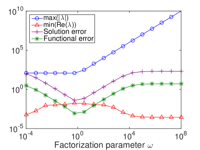
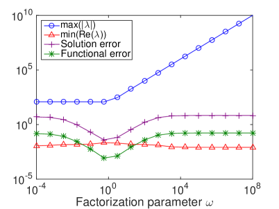
Remark 5.1.

When we have a hyperbolic problem, step (i) is omitted and step (iv) is modified such that the scheme (17) is used with penalty parameters given in Theorem 2.6.

In the simulations, we are interested in the functional error $\mathtt{E}=J(U)-\mathcal{J}(\hskip 1.0pt\mathcal{U})$, where $\mathcal{J}(\hskip 1.0pt\mathcal{U})=\langle{\mathcal{G},\hskip 1.0pt\mathcal{U}}\rangle$, $J(U)=\langle{G,U}\rangle_{{}_{H}}$ and $G_{i}(t)=\mathcal{G}(x_{i},t)$, but of course also in the solution error $\mathtt{e}$, where $\mathtt{e}_{i}(t)=U_{i}(t)-\hskip 1.0pt\mathcal{U}(x_{i},t)$. We also investigate the spectra of $L$, that is the eigenvalues $\lambda_{j}$ of $L,$ with $j=1,2,\ldots,n(N+1)$. Here we are in particular interested in the spectral radius $\rho=\max_{j}(|\lambda_{j}|)$ and in $\eta=\min_{j}(\Re(\lambda_{j}))$. (For time-dependent problems $\rho\Delta t\lesssim C$ is a crude estimate of the stability regions of explicit Runge-Kutta schemes, and thus $\rho$ can be seen as a measure of stiffness. The eigenvalue with the smallest real part, $\eta$, determines how fast a time-dependent solution converges to a steady-state solution, see [14].) Ideally, the penalties are chosen such that $\rho$ is kept small while $\eta$ is maximized. For steady problems or when using implicit time solvers, other properties (e.g. the condition number) might be of greater interest.

We start by investigating a couple of scalar cases in some detail, then give an example of a system with a solid wall type of boundary condition.

5.1 The scalar case

Consider the scalar advection-diffusion equation,

$$\begin{array}[]{rll}\hskip 1.0pt\mathcal{U}_{t}+a\hskip 1.0pt\mathcal{U}_{x}-\varepsilon\hskip 1.0pt\mathcal{U}_{xx}=&\mathcal{F},&x\in[0,1],\vspace{4pt}\\ \alpha_{{}_{L}}\hskip 1.0pt\mathcal{U}+\beta_{{}_{L}}\hskip 1.0pt\mathcal{U}_{x}=&g_{\scalebox{0.6}{$L$\hskip 1.0pt}},&x=0,\vspace{4pt}\\ \alpha_{{}_{R}}\hskip 1.0pt\mathcal{U}+\beta_{{}_{R}}\hskip 1.0pt\mathcal{U}_{x}=&g_{\scalebox{0.6}{$R$\hskip 1.0pt}},&x=1,\end{array}$$ (107)

valid for $t\geq 0$, with initial condition $\hskip 1.0pt\mathcal{U}(x,0)=\hskip 1.0pt\mathcal{U}_{0}(x)$ and where $\varepsilon>0$. Using (65) yields

$$\hskip 3.0pt\overline{\mathcal{A}\hskip 0.5pt}=\left[\begin{array}[]{cc}a&-\varepsilon\\ -\varepsilon&0\end{array}\right], \hskip 1.0pt\overline{\mathcal{B}\hskip 1.0pt}_{L}=\left[\begin{array}[]{cc}\alpha_{{}_{L}}&\beta_{{}_{L}}\end{array}\right], \hskip 1.0pt\overline{\mathcal{B}\hskip 1.0pt}_{R}=\left[\begin{array}[]{cc}\alpha_{{}_{R}}&\beta_{{}_{R}}\end{array}\right].$$

In this case, the factorization of the matrix $\hskip 3.0pt\overline{\mathcal{A}\hskip 0.5pt}$ can be parameterized as

$$\hskip 3.0pt\overline{\mathcal{A}\hskip 0.5pt}=\hskip 2.0pt\overline{Z}\hskip 1.0pt\overline{\Delta}\hskip 1.0pt\hskip 2.0pt\overline{Z}^{T}=\left[\begin{array}[]{cc}\frac{a+\omega}{2s_{1}}&\frac{a-\omega}{2s_{2}}\\ \frac{-\varepsilon}{s_{1}}&\frac{-\varepsilon}{s_{2}}\end{array}\right]\left[\begin{array}[]{cc}\frac{s_{1}^{2}}{\omega}&0\\ 0&-\frac{s_{2}^{2}}{\omega}\end{array}\right]\left[\begin{array}[]{cc}\frac{a+\omega}{2s_{1}}&\frac{a-\omega}{2s_{2}}\\ \frac{-\varepsilon}{s_{1}}&\frac{-\varepsilon}{s_{2}}\end{array}\right]^{T},$$ (114)

with $\omega>0$. In particular, if $\omega=\sqrt{a^{2}+4\varepsilon^{2}}$ and if $s_{1,2}^{2}=\omega(\omega\pm a)/2$, then the above factorization is the eigendecomposition of $\hskip 3.0pt\overline{\mathcal{A}\hskip 0.5pt}$. The discrete scheme mimicking (107) is

$$\begin{split}U_{t}+aD_{1}U-\varepsilon D_{2}U=F&+H^{-1}(\mu_{0}e_{0}+\nu_{\hskip 0.5pt0\hskip 0.5pt}S^{T}e_{0})\left(\alpha_{{}_{L}}U_{0}+\beta_{{}_{L}}(SU)_{0}-g_{\scalebox{0.6}{$L$\hskip 1.0pt}}\right)\\ &+H^{-1}(\mu_{N}e_{N}+\nu_{N}S^{T}e_{N})\left(\alpha_{{}_{R}}U_{N}+\beta_{{}_{R}}(SU)_{N}-g_{\scalebox{0.6}{$R$\hskip 1.0pt}}\right).\end{split}$$ (115)

To compute the penalty parameters, $\hskip 2.0pt\overline{P\hskip 1.0pt}_{L}=\frac{s_{1}}{\omega}\left(\alpha_{{}_{L}}+\beta_{{}_{L}}\frac{a-\omega}{2\varepsilon}\right)$ and $\hskip 2.0pt\overline{P\hskip 1.0pt}_{R}=-\frac{s_{2}}{\omega}\left(\alpha_{{}_{R}}+\beta_{{}_{R}}\frac{a+\omega}{2\varepsilon}\right)$ are needed, which we obtain using (103). Theorem 3.2 now yields

$$\begin{split}\mu_{0}&=\frac{-\frac{a+\omega}{2}-q\varepsilon}{\alpha_{{}_{L}}+\beta_{{}_{L}}\frac{a-\omega}{2\varepsilon}-q\beta_{{}_{L}}},\hskip 45.0pt\nu_{\hskip 0.5pt0\hskip 0.5pt}=\frac{-\varepsilon}{\alpha_{{}_{L}}+\beta_{{}_{L}}\frac{a-\omega}{2\varepsilon}-q\beta_{{}_{L}}},\\ \mu_{N}&=\frac{\frac{a-\omega}{2}-q\varepsilon}{\alpha_{{}_{R}}+\beta_{{}_{R}}\frac{a+\omega}{2\varepsilon}+q\beta_{{}_{R}}},\hskip 41.0pt\nu_{N}=\frac{\varepsilon}{\alpha_{{}_{R}}+\beta_{{}_{R}}\frac{a+\omega}{2\varepsilon}+q\beta_{{}_{R}}}.\end{split}$$ (116)

Formally $0<\omega<\infty$ is necessary (since in the limits $\hskip 2.0pt\overline{Z}$ becomes singular), but as long as the number of imposed boundary condition does not change or the penalty parameters go to infinity, we can allow $0\leq\omega\leq\infty$. Below we present some special cases:

For Dirichlet boundary conditions we have $\alpha_{{}_{L}}=\alpha_{{}_{R}}=1$ and $\beta_{{}_{L}}=\beta_{{}_{R}}=0$. In this case the penalty parameters in (116) become

$$\mu_{0} =-\frac{a+\omega}{2}-q\varepsilon, \nu_{\hskip 0.5pt0\hskip 0.5pt} =-\varepsilon, \mu_{N} =\frac{a-\omega}{2}-q\varepsilon, \nu_{N} =\varepsilon,$$ (117)

with $0\leq\omega<\infty$. Translating the penalty parameters for the advection-diffusion case in [1] to the form used here, it can be seen that they are exactly the same.

With $\alpha_{{}_{L}}=\frac{|a|+a}{2}$, $\beta_{{}_{L}}=-\varepsilon$ at the left boundary and $\alpha_{{}_{R}}=\frac{|a|-a}{2}$, $\beta_{{}_{R}}=\varepsilon$ at the right boundary, we have boundary conditions of a low-reflecting far-field type. In this case, the penalty parameters in (116) become

$$\mu_{0} =-\frac{\frac{\omega+a}{2}+q\varepsilon}{\frac{\omega+|a|}{2}+q\varepsilon}, \nu_{\hskip 0.5pt0\hskip 0.5pt}=\frac{-\varepsilon}{\frac{\omega+|a|}{2}+q\varepsilon}, \mu_{N} =-\frac{\frac{\omega-a}{2}+q\varepsilon}{\frac{\omega+|a|}{2}+q\varepsilon}, \nu_{N}=\frac{\varepsilon}{\frac{\omega+|a|}{2}+q\varepsilon}$$ (118)

and we see that in the limit $\omega\to\infty$, we obtain $\mu_{0}=-1$, $\nu_{\hskip 0.5pt0\hskip 0.5pt}=0$, $\mu_{N}=-1$ and $\nu_{N}=0$. This particular choice corresponds to the penalty $\Sigma=-I$ used in [2, 3] for systems with boundary conditions of far-field type.

Remark 5.2.

If $\varepsilon=0$ in (107) we get the transport equation, and then only one boundary condition should be given instead of two. That means that the derivation of the penalty parameters must be redone accordingly. See [1], where this case is covered.

Remark 5.3.

The results can be extended to the case of varying coefficients. Consider the scalar diffusion problem $\hskip 1.0pt\mathcal{U}_{t}-(\varepsilon\hskip 1.0pt\mathcal{U}_{x})_{x}=\mathcal{F}$ with Dirichlet boundary conditions, where $\varepsilon(x)>0$. Following [12], we define a narrow-stencil operator mimicking $\partial/\partial x(\varepsilon\partial/\partial x)$ as

$$D_{2}^{(\varepsilon)}=H^{-1}\left(-A_{\scalebox{0.7}{$S$\hskip 1.0pt}}^{(\varepsilon)}+(\varepsilon(1)E_{N}-\varepsilon(0)E_{0})S\right)$$

where $A_{\scalebox{0.7}{$S$\hskip 1.0pt}}^{(\varepsilon)}$ is symmetric and positive semi-definite. It is assumed that $D_{2}^{(\varepsilon)}=\varepsilon D_{2}$ holds when $\varepsilon$ is constant. The discrete problem becomes

$$U_{t}-D_{2}^{(\varepsilon)}U=F+H^{-1}(\mu_{0}e_{0}+\nu_{\hskip 0.5pt0\hskip 0.5pt}S^{T}e_{0})\left(U_{0}-g_{\scalebox{0.6}{$L$\hskip 1.0pt}}\right)+H^{-1}(\mu_{N}e_{N}+\nu_{N}S^{T}e_{N})\left(U_{N}-g_{\scalebox{0.6}{$R$\hskip 1.0pt}}\right).$$

The continuous problem is self-adjoint, so for dual consistency $L^{*}=H^{-1}L^{T}H=L$ is needed, which is fulfilled if $\nu_{\hskip 0.5pt0\hskip 0.5pt}=-\varepsilon(0)$ and $\nu_{N}=\varepsilon(1)$. Moreover, using $A_{\scalebox{0.7}{$S$\hskip 1.0pt}}^{(\varepsilon)}\geq\varepsilon_{\min}A_{\scalebox{0.7}{$S$\hskip 1.0pt}}$, where $\varepsilon_{\min}=\min_{x\in[0,1]}\varepsilon(x)$, it can be shown that the discretization will be stable if we choose $\mu_{0}\leq-\frac{q}{\varepsilon_{\min}}\varepsilon(0)^{2}$ and $\mu_{N}\leq-\frac{q}{\varepsilon_{\min}}\varepsilon(1)^{2}$. (The superconvergence for functionals has been confirmed numerically and the resulting ”best” choices of $\mu_{0}$ and $\mu_{N}$ are similar to what we obtain in the constant case considered below.)

5.1.1 The stationary heat equation with Dirichlet boundary conditions

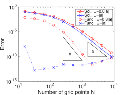
We consider the heat equation with Dirichlet boundary conditions, i.e. problem (107) with $a=0$, $\alpha_{{}_{L}},\alpha_{{}_{R}}=1$ and $\beta_{{}_{L}},\beta_{{}_{R}}=0$, which we solve using the scheme (115), with the penalty parameters given by (117), also with $a=0$. To isolate the errors originating from the spatial discretization, we first look at the steady problem. Thus we let $\hskip 1.0pt\mathcal{U}_{t}=0$ and solve $-\hskip 1.0pt\mathcal{U}_{xx}=\mathcal{F}(x)$ numerically. The resulting quantities $\rho$ and $\eta$, the solution error $\|\mathtt{e}\|_{{}_{H}}$ and the functional error $|\mathtt{E}|$ are given (as functions of the parameter $\omega$) in Figure 1. The spectral radius $\rho$ grows with $\omega$, so we do not want $\omega\to\infty$. On the other hand, the decay rate $\eta$ shrinks with $\omega$ so $\omega\to 0$ should also be avoided. The errors tend to decrease with increasing $\omega$ (the errors naturally varies slightly depending on the choice of $\mathcal{F}$ and $\mathcal{G}$, but the example in Figure 1 shows a typical behavior). Thus the demand for accuracy is conflicting with the demand of keeping $\rho$ small (the aim to maximize $\eta$ is met before the aim to minimize the errors and is therefore not a limiting factor in this case). Empirically we have found that a good compromise, which gives small errors without increasing the spectral radius dramatically, is obtained using $\omega\approx q\varepsilon$.

(a) Interior order 6, wide operator

(b) Interior order 6, narrow operator

Figure 1: Properties of $L$ and errors when solving $-\hskip 1.0pt\mathcal{U}_{xx}=\mathcal{F}(x)$ with Dirichlet boundary conditions. The number of grid points is $N=64$, the second derivative operator is 6th order accurate in the interior, and is either wide or narrow. Here $\hskip 1.0pt\mathcal{U}(x)=\mathcal{G}(x)=\cos(30x)$.

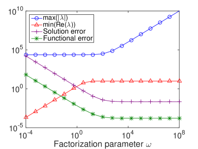
From this example, we make an observation. If we would use the eigenfactorization, we would have $\omega=\sqrt{a^{2}+4\varepsilon^{2}}=2$. However, in Figure 1 we see that that choice is not especially good, since the errors then become much larger than if using $\omega=q\varepsilon$, which is approximately 200 and 340, respectively. In some cases, the difference in accuracy is so severe that the choice of factorization parameter $\omega$ affects the convergence rate. For the narrow operator with the order (2,0), the errors behave as $\|\mathtt{e}\|_{{}_{H}}\sim h^{3/2}$ when using $\omega\sim 1$, whereas we obtain the expected $\|\mathtt{e}\|_{{}_{H}}\sim h^{2}$ when using $\omega\sim 1/h$. Similar behaviors are observed also for narrow operators of higher order, see below.

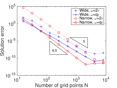
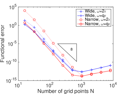
In Figure 2(a) the errors $\|\mathtt{e}\|_{{}_{H}}$ for the operators with interior order 6 are shown. For the narrow scheme, the convergence rate is 4.5 when using $\omega=2\varepsilon$ and 5.5 when using $\omega=q\varepsilon$. For the wide scheme, the order is 4 in both cases, but the error constant changes. In the 8th order case, Figure 2(b), the convergence rates are not affected, but in the narrow case the errors are around 2500 times smaller when using $\omega=q\varepsilon$. In this example, the functional errors are not as sensitive to $\omega$ as the solution errors. In the 6th order case, the convergence rates are slightly better than the predicted $2p=6$, both for the wide and the narrow schemes, see Figure 3(a). For the 8th order case, see Figure 3(b), the convergence rates are in all cases higher than $2p=8$. Thus the derived SAT parameters actually produce superconvergent functionals, also for the narrow operators.

(a) Interior order 6

(b) Interior order 8

Figure 2: The error $\|\mathtt{e}\|_{{}_{H}}$, for $-\hskip 1.0pt\mathcal{U}_{xx}=\mathcal{F}(x)$. The exact solution is $\hskip 1.0pt\mathcal{U}=\cos(30x)$.

(a) Interior order 6

(b) Interior order 8

Figure 3: The functional error $|\mathtt{E}|$, using the weight function $\mathcal{G}(x)=\cos(30x)$.

5.1.2 The time-dependent heat equation with Dirichlet boundary conditions

Next, we consider the actual heat equation. We solve $\hskip 1.0pt\mathcal{U}_{t}=\varepsilon\hskip 1.0pt\mathcal{U}_{xx}+\mathcal{F}(x,t)$ with $\varepsilon=0.01$ and the exact solution $\hskip 1.0pt\mathcal{U}(x,t)=\cos(30x)+\sin(20x)\cos(10t)+\sin(35t)$. For the time propagation the classical 4th order accurate Runge-Kutta scheme is used, with sufficiently small time steps, $\Delta t=10^{-4}$, such that the spatial errors dominate. In Figure 4 the errors obtained using the narrow (6,3) order scheme are shown as a function of time.

(a) Solution error $\|\mathtt{e}\|_{{}_{H}}$

(b) Functional error $|\mathtt{E}|$ with $\mathcal{G}(x)=1$

Figure 4: Errors when solving the heat equation using the narrow (6,3) order scheme.

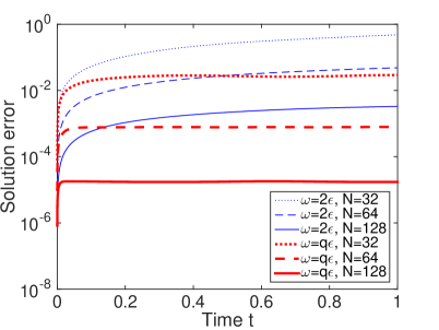
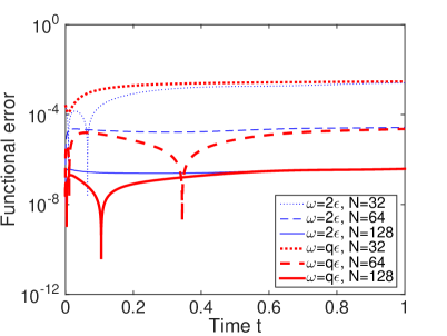
The corresponding spatial order of convergence (at time $t=1$) is shown in Table 2. The simulations confirm the steady results, namely that both $\omega=2\varepsilon$ and $\omega=q\varepsilon$ give superconvergent functionals but that choosing the factorization parameter as $\omega\sim\varepsilon/h$ improves the solution significantly compared to when using the eigendecomposition.

$\begin{array}[]{|r|cccc|cccc|}\hline\cr&\vrule\lx@intercol\hfil\omega=2\varepsilon\hfil\lx@intercol\vrule\lx@intercol&\vrule\lx@intercol\hfil\omega=q\varepsilon\hfil\lx@intercol\vrule\lx@intercol\\ N&\|\mathtt{e}\|_{{}_{H}}&\text{Order}&|\mathtt{E}|&\text{Order}&\|\mathtt{e}\|_{{}_{H}}&\text{Order}&|\mathtt{E}|&\text{Order}\\ \hline\cr 32&0.480872&-&0.00258741&-&0.029297&-&0.00297573&-\\ 64&0.048501&3.3096&0.00002704&6.5804&0.000790&5.2121&0.00002315&7.0064\\ 128&0.003307&3.8743&0.00000038&6.1559&0.000017&5.5131&0.00000039&5.9055\\ \hline\cr\end{array}$

Table 2: The errors and convergence rates at $t=1$ for the narrow (6,3) order scheme.

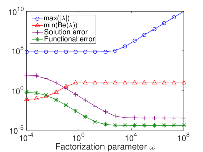
5.1.3 The heat equation with Neumann boundary conditions

We solve $\hskip 1.0pt\mathcal{U}_{t}=\varepsilon\hskip 1.0pt\mathcal{U}_{xx}+\mathcal{F}(x,t)$ again, but this time with Neumann boundary conditions, and the penalty parameters are now given by (116) with $a=0$, $\varepsilon=0.01$, $\alpha_{{}_{L}}=\alpha_{{}_{R}}=0$ and $\beta_{{}_{L}}=\beta_{{}_{R}}=1$. In contrast to when having Dirichlet boundary conditions, the spectral radius $\rho$ does not depend so strongly on $\omega$ and therefore we can let $\omega\to\infty$. Figure 5 shows the convergence rates for the schemes with interior order 6. The exact solution is $\hskip 1.0pt\mathcal{U}(x,t)=\cos(30x)$ and for the time propagation the implicit Euler method, with $\Delta t=1$, is used (this is more than enough since the chosen $\hskip 1.0pt\mathcal{U}$ does not depend on $t$). We note that the convergence rates behaves similarly to the Dirichlet case. We could also have used $\omega=q\varepsilon$ here, it gives the same convergence rates as $\omega=\infty$.

(a) Solution error $\|\mathtt{e}\|_{{}_{H}}$

(b) Functional error $|\mathtt{E}|$ with $\mathcal{G}(x)=\cos(30x)$

Figure 5: Errors at time $t=100$ when solving the heat equation with Neumann boundary conditions using the schemes with interior order 6.

5.1.4 The advection-diffusion equation with Dirichlet boundary conditions

For simplicity we consider steady problems again, this time $a\hskip 1.0pt\mathcal{U}_{x}=\varepsilon\hskip 1.0pt\mathcal{U}_{xx}+\mathcal{F}$. That is, we solve (107) using the scheme (115), both with omitted time derivatives. The penalty parameters for Dirichlet boundary conditions are given in (117).

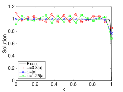
First, we take a look at an interesting special case, namely when $\mathcal{F}=0$. Then the exact solution is $\hskip 1.0pt\mathcal{U}(x)=c_{1}+c_{2}\exp{(ax/\varepsilon)}$, where the constants $c_{1}$ and $c_{2}$ are determined by the boundary conditions. For $\varepsilon\ll|a|$ the exact solution forms a thin boundary layer at the outflow boundary, which for insufficient resolution usually leads to oscillations in the numerical solution. This can be handled by upwinding or artificial diffusion (see e.g. [16]). Here we will instead use the free parameter $\omega$ in the penalty to minimize the oscillating modes (the so-called $\pi$-modes).

We start with the wide second derivatives stencils. The ansatz $U_{i}=k^{i}$, inserted into the interior of the scheme (115), gives (for the second order case) a numerical solution

$$U_{i}=\widetilde{c}_{1}+\widetilde{c}_{2}(-1)^{i}+\widetilde{c}_{3}k_{3}^{i}+\widetilde{c}_{4}k_{4}^{i}, \ k_{3,4}=\frac{ha}{\varepsilon}\pm\sqrt{\frac{h^{2}a^{2}}{\varepsilon^{2}}+1}.$$

Thus there exist two modes with alternating signs, $\widetilde{c}_{2}(-1)^{i}$ and $\widetilde{c}_{4}k_{4}^{i}$. However, one can show that the choice $\omega=|a|$ leads to $\widetilde{c}_{2}=0$ and to $\widetilde{c}_{4}$ being small enough compared to $\widetilde{c}_{3}$ such that $U_{i}$ is monotone. Empirically we have seen that this nice behavior holds also for the wide schemes with higher order of accuracy. In Figure 6 the result using the scheme with interior order 8 is shown. The solution obtained using $\omega=|a|$ shows no oscillations, even though the grid is very coarse. Moreover, this particular choice of factorization gives functional errors almost at machine precision (although it should be noted that this is a special case since $\mathcal{F}(x)=0$ and $\mathcal{G}(x)=1$).

(a) The number of grid points is $N=16$.

(b) The weight function is $\mathcal{G}(x)=1$.

Figure 6: We solve $a\hskip 1.0pt\mathcal{U}_{x}=\varepsilon\hskip 1.0pt\mathcal{U}_{xx}$ with $a=1$, $\varepsilon=0.005$ using the wide scheme with interior order 8. In a) the solutions, in b) the errors $\|\mathtt{e}\|_{{}_{H}}$ and $|\mathtt{E}|$.

For the narrow-stencil schemes, the existence of spurious oscillating modes depends on the resolution. In the second order case, the interior solution is

$$U_{i}=\widetilde{\widetilde{c}}_{1}+\widetilde{\widetilde{c}}_{2}\left(\frac{1+ah/(2\varepsilon)}{1-ah/(2\varepsilon)}\right)^{i},$$

which has an oscillating component if $|a|h/(2\varepsilon)>1$. With very particular choices of the penalty parameter this component can be canceled (for the operators with order (2,0) and (2,1) it is achieved using $\omega=|a|/(1-\frac{2\varepsilon}{|a|h})$ and $\omega=|a|(1-\frac{\varepsilon}{|a|h})/(1-\frac{2\varepsilon}{|a|h})^{2}$, respectively) such that the numerical solution becomes constant. As soon as $|a|h/(2\varepsilon)<1$, this mode should not be canceled anymore, but how to do the transition between the unresolved case and the resolved case is not obvious. For the higher order schemes the $\omega$ which cancels the oscillating modes are even more complicated and in some cases negative (i.e. useless). In short, these particular, canceling choices of $\omega$ are not worth the effort. Instead, we recommend to use $\omega\approx|a|+q\varepsilon$ for the narrow-stencil operators, see below.

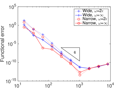
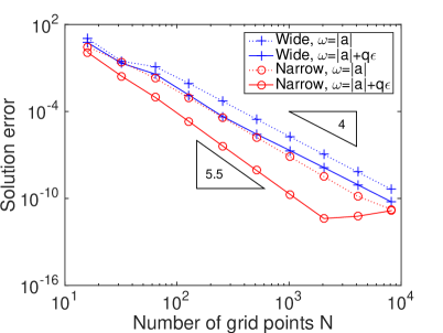
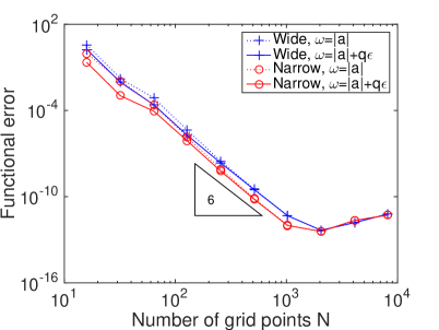
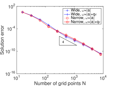
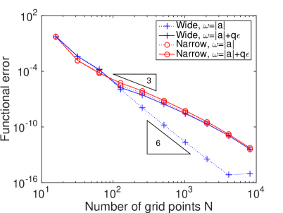
The above results were obtained under the assumption $\mathcal{F}=0$. Next, we use a forcing function $\mathcal{F}$ such that the exact solution is $\hskip 1.0pt\mathcal{U}(x)=\cos(30x)$. The resulting errors, together with $\rho$ and $\eta$, are shown in Figure 7 for $a=1$ and $\varepsilon=10^{-6}$. Clearly, $\omega\approx|a|$ is still a good choice since the errors are small, $\rho$ is not too large and $\eta$ is maximal. For $\varepsilon\gg|a|h$ the curves are more similar to those in Figure 1, and $\omega\approx|a|+q\varepsilon$ will be a better choice. In the transition region $\varepsilon\sim|a|h$ we sometimes observe order reduction. This can be seen in Figures 8 and 9 for the schemes with an interior order of accuracy 6. Figure 8 shows the convergence rates when $\varepsilon=0.1$, which is large enough for the numerical solution to be well resolved. For the narrow scheme, we see an improved convergence rate for the solution error if $\omega=|a|+q\varepsilon$ is used. The functional output converges with $2p=6$ for all schemes. Figure 9 shows the convergence rates when $\varepsilon$ is decreased to $10^{-4}$, such that the numerical solution is badly resolved. For all schemes, except the wide scheme with the particular choice $\omega=|a|$, we see a pre-asymptotic order reduction of the functional.

(a) Wide-stencil second derivative

(b) Narrow-stencil second derivative

Figure 7: We solve $a\hskip 1.0pt\mathcal{U}_{x}=\varepsilon\hskip 1.0pt\mathcal{U}_{xx}+\mathcal{F}(x)$ with Dirichlet boundary conditions and with $\hskip 1.0pt\mathcal{U}(x)=\mathcal{G}(x)=\cos(30x)$. The number of grid points is $N=64$, the interior order is 6.

We conclude that the penalties in Theorem 3.2 yields superconvergent functionals for the advection-diffusion equation with Dirichlet boundary conditions – in the asymptotic limit. In the special case when having the wide scheme with $\omega=|a|$ we even get super-convergent functionals in the troublesome transition region.

Figure 8: The inner order of accuracy is 6, $\hskip 1.0pt\mathcal{U}(x)=\mathcal{G}(x)=\cos(30x)$, $a=1$ and $\varepsilon=0.1$.

Figure 9: The inner order of accuracy is 6, $\hskip 1.0pt\mathcal{U}(x)=\mathcal{G}(x)=\cos(30x)$, $a=1$ and $\varepsilon=10^{-4}$.

5.1.5 The advection-diffusion equation with far-field boundary conditions

We just comment briefly on the far-field boundary conditions and their corresponding SAT parameters given in (118). If $|a|h/\varepsilon$ is large, the quantities $\rho$, $\eta$ and the errors barely depend on $\omega$ (except if $\mathcal{F}=0$, then the errors are smaller if $\omega\approx|a|$). For small $|a|h/\varepsilon$, large values of $\omega$ give smaller errors and slightly larger $\eta$, whereas $\rho$ is slightly increased. In this case, the penalty obtained by taking the limit $\omega\to\infty$, that is $\mu_{0}=-1$, $\nu_{\hskip 0.5pt0\hskip 0.5pt}=0$, $\mu_{N}=-1$ and $\nu_{N}=0$ (corresponding to the penalty used in [2, 3]) is not a bad choice and it has an appealing simplicity. As before, $\omega\approx|a|+q\varepsilon$ also gives good results.

5.1.6 Reflections from the scalar case

From what we have seen from the numerical experiments so far, the best choice of the factorization parameter $\omega$ is not only dependent on the continuous problem at hand (i.e. the parameters $a$ and $\varepsilon$ and the type of boundary conditions), but also on numerical quantities, such as the grid resolution and if the stencils are wide or narrow. In some cases the factorization has almost no impact, sometimes it makes the system at hand extremely ill-conditioned or even changes the order of accuracy of the scheme.

In the scalar case it is rather straightforward to optimize with respect to the single factorization parameter $\omega$, but for systems this task becomes non-trivial and one might have to settle for the factorizations at hand. Nevertheless, we note that the eigendecomposition is not necessarily the best factorization and that it could be worth searching for other options. With that being said, next we consider a system and use nothing but the eigendecomposition for constructing the penalty parameters.

5.2 A fluid dynamics system with solid wall boundary conditions

The symmetrized, compressible Navier–Stokes equations in one dimension ($\Omega=[0,1]$) with frozen coefficients is given by (47), with

$$\mathcal{A}=\left[\begin{array}[]{ccc}\bar{u}&a&0\\ a&\bar{u}&b\\ 0&b&\bar{u}\end{array}\right], \mathcal{E}=\varepsilon\left[\begin{array}[]{ccc}0&0&0\\ 0&\varphi&0\\ 0&0&\psi\end{array}\right], \hskip 1.0pt\mathcal{U}=\left[\begin{array}[]{c}\varrho\\ u\\ T\end{array}\right],$$

where the constants $\bar{u}$, $a$, $b$, $\varepsilon$, $\varphi$ and $\psi$ denote suitable physical quantities and where $\varrho$, $u$ and $T$ are scaled perturbations in density, velocity and temperature. Let $\bar{u}<0$ and $\varepsilon,\varphi,\psi>0$. In this case, two boundary conditions should be given at the left boundary and three at the right boundary. We impose solid wall boundary conditions (a perfectly insulated wall) at the left boundary, that is $u(0,t)=T_{x}(0,t)=0$. At the right boundary, we impose free stream boundary conditions of Dirichlet type, as $\hskip 1.0pt\mathcal{U}(1,t)=\hskip 1.0pt\mathcal{U}_{\infty}$. These boundary conditions give a well-posed problem. The boundary operators are

$$\mathcal{H}_{L} =\left[\begin{array}[]{ccc}0&1&0\\ 0&0&0\end{array}\right], \mathcal{G}_{L} =\left[\begin{array}[]{ccc}0&0&0\\ 0&0&1\end{array}\right], \mathcal{H}_{R} =\left[\begin{array}[]{ccc}1&0&0\\ 0&1&0\\ 0&0&1\end{array}\right], \mathcal{G}_{R} =\left[\begin{array}[]{ccc}0&0&0\\ 0&0&0\\ 0&0&0\end{array}\right].$$

These boundary conditions can not be rearranged to the far-field form and therefore the penalty used in [2, 3] can not be applied. We identify $\hskip 3.0pt\overline{\mathcal{A}\hskip 0.5pt}$, $\hskip 1.0pt\overline{\mathcal{B}\hskip 1.0pt}_{L}$ and $\hskip 1.0pt\overline{\mathcal{B}\hskip 1.0pt}_{R}$ according to (65), and factorize $\hskip 3.0pt\overline{\mathcal{A}\hskip 0.5pt}$ using the eigendecomposition. The dual consistent penalty parameters are now described in (80), with

$$\hskip 1.5pt\mathcal{K}_{L} =\left[\begin{array}[]{ccc}0&0&0\\ 0&0&1/(\varepsilon\psi)\end{array}\right], \hskip 1.5pt\mathcal{K}_{R} =\left[\begin{array}[]{ccc}0&0&0\\ 0&0&0\\ 0&0&0\end{array}\right].$$

As a comparison, we use the alternative penalty parameters (cf. Method 2 in Remark 4.3)

$$\tilde{\mu}_{0}=\left[\begin{array}[]{cc}-a&0\\ 0&0\\ -b&\varepsilon\psi\end{array}\right], \tilde{\nu}_{0}=\left[\begin{array}[]{cc}0&0\\ \varepsilon\varphi&0\\ 0&0\end{array}\right], \tilde{\mu}_{N}=\left[\begin{array}[]{ccc}\bar{u}&a&0\\ 0&\bar{u}&0\\ 0&b&\bar{u}\end{array}\right], \tilde{\nu}_{N}=\left[\begin{array}[]{ccc}0&0&0\\ 0&-\varepsilon\varphi&0\\ 0&0&-\varepsilon\psi\end{array}\right]$$

which give stability (they are chosen such that the boundary terms in (82) are non-positive for zero data) but they do not fulfill the demands for dual consistency.

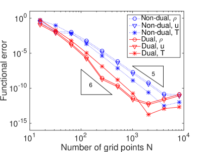
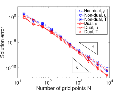
In the numerical simulations we use the exact solution $\varrho=\cos(7x)$, $u=\sin(13x)$ and $T=\cos(30x)$ and as weight functions we use $\mathcal{G}(x)=[1,\ 0,\ 0]^{T}$, $\mathcal{G}(x)=[0,\ 1,\ 0]^{T}$ and $\mathcal{G}(x)=[0,\ 0,\ 1]^{T}$ (such that one functional output is obtained for each variable). Figure 10 shows the resulting errors when using the schemes with interior order 6. In the wide case, the solutions do not differ much. In the narrow case, the dual consistent solution converges one half order slower than the dual inconsistent one (order 4 for $\varrho$ and 4.5 for $u,T$ compared to 4.5 for $\varrho$ and 5 for $u,T$), but the result is still as good as in the wide case. Moreover, recall that in the scalar case the order could be improved by choosing another factorization than the eigendecomposition, see Figure 8(a). In Figure 11 we see that the functionals convergence with the expected 6th order for both the dual consistent schemes, whereas the dual inconsistent schemes yield 5th order.

(a) Interior order 6, wide operator

(b) Interior order 6, narrow operator

Figure 10: Solution errors, for $\bar{u}=-0.5$, $a=0.8$, $b=0.6$, $\varphi=1$, $\psi=2$, $\varepsilon=0.01$.

(a) Interior order 6, wide operator

(b) Interior order 6, narrow operator

Figure 11: Functional errors, for $\bar{u}=-0.5$, $a=0.8$, $b=0.6$, $\varphi=1$, $\psi=2$, $\varepsilon=0.01$.

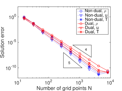
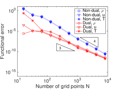
The diffusion parameter is decreased from $\varepsilon=0.01$ to $\varepsilon=10^{-6}$ and the resulting errors are shown in Figures 12 and 13. Now the solution errors obtained using the dual consistent schemes are slightly better than the ones obtained using the dual inconsistent schemes, but the difference is small, see Figure 12.

(a) Interior order 6, wide operator

(b) Interior order 6, narrow operator

Figure 12: Solution errors, for $\bar{u}=-0.5$, $a=0.8$, $b=0.6$, $\varphi=1$, $\psi=2$, $\varepsilon=10^{-6}$.

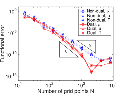
For the functional errors the difference is more pronounced, see Figure 13. In the wide case, the dual consistent scheme produces a perfect convergence rate of almost 7. This behavior was observed already in the scalar case, when the factorization parameter was chosen exactly as $\omega=|a|$ (which for small amounts of diffusion is very close to the eigendecomposition). For the narrow-stencil schemes the dual consistent scheme still produces smaller errors than the dual inconsistent scheme, but the order is reduced to 3 (a pre-asymptotic low-order tendency seen already in Figure 9 in the scalar case).

(a) Interior order 6, wide operator

(b) Interior order 6, narrow operator

Figure 13: Functional errors, for $\bar{u}=-0.5$, $a=0.8$, $b=0.6$, $\varphi=1$, $\psi=2$, $\varepsilon=10^{-6}$.

Extrapolating from the scalar case, we assume that it could be worth searching for better penalty parameters for the narrow-stencil schemes when having diffusion dominated problems. However, for convection dominated problems the wide scheme with a factorization close to the eigendecomposition is hard to beat.

6 Concluding remarks

We use a finite difference method based on summation by parts operators, combined with a penalty method for the boundary conditions (SBP-SAT). Diagonal-norm SBP operators have $2p$-order accurate interior stencils and $p$-order accurate boundary closures, which limits the global accuracy of the solution to $p+1$ (or $p+2$ for parabolic problems under certain conditions). Recently, it has been shown that SBP-SAT schemes can give functional estimates that are $\mathcal{O}(h^{2p})$. To achieve this superconvergence, the SAT parameters must be carefully chosen to ensure that the discretization is dual-consistent.

We first look at hyperbolic systems and derive stability requirements and duality constraints for the SATs. Then we present a recipe to choose these SAT parameters such that both these (independent) demands are fulfilled. When wide-stencil second derivative operators are used, the results automatically extend to parabolic problems. We generalize the recipe such that it holds also for narrow-stencil second derivative operators.

The $2p$ order convergence of SBP-SAT functional estimates is confirmed numerically for a variety of scalar examples, as well as for an incompletely parabolic system. For low-diffusion advection-diffusion problems, the superconvergence is sometimes seen first asymptotically. Generally speaking, the narrow-stencil schemes are better for diffusion dominated problems whereas the wide schemes are preferable for advection dominated problems.

In most cases the derived dual consistent SAT parameters have some remaining degree of freedom. The free parameters can be used to improve the accuracy of the primary solution or to tune numerical quantities such as spectral radius, decay rate or condition numbers. Optimal choices within these families are suggested for the scalar problems, however, to do the same for systems is considered a task for the future.

Appendix A Reformulation of the first order form discretization

We derive the scheme (66) with penalty parameters (68), using the hyperbolic results.

Step 1: Consider the problem (51), which is a first order system. We represent the solution $\hskip 2.0pt\overline{\hskip 1.0pt\mathcal{U}}$ by a discrete solution vector $\hskip 1.0pt\overline{U}=[\hskip 1.0pt\overline{U}_{0}^{T},\hskip 1.0pt\overline{U}_{1}^{T},\ldots,\hskip 1.0pt\overline{U}_{N}^{T}]^{T}$, where $\hskip 1.0pt\overline{U}_{i}(t)\approx\hskip 2.0pt\overline{\hskip 1.0pt\mathcal{U}}(x_{i},t)$ and discretize (51) exactly as was done in (17) for the hyperbolic case, that is as

$$\begin{split}(I_{N}\otimes\overline{\mathcal{I}})\hskip 1.0pt\overline{U}_{t}+(I_{N}\otimes\hskip 1.0pt\overline{\mathcal{R}\hskip 0.5pt})\hskip 1.0pt\overline{U}+(D_{1}\otimes\hskip 3.0pt\overline{\mathcal{A}\hskip 0.5pt})\hskip 1.0pt\overline{U}=\hskip 2.0pt\overline{F}&+(H^{-1}e_{0}\otimes\overline{\Sigma}_{\hskip 1.0pt0\hskip 0.5pt})(\hskip 1.0pt\overline{\mathcal{B}\hskip 1.0pt}_{L}{\hskip 1.0pt\overline{U}}_{0}-g_{\scalebox{0.6}{$L$\hskip 1.0pt}})\\ &+(H^{-1}e_{N}\otimes\overline{\Sigma}_{N})(\hskip 1.0pt\overline{\mathcal{B}\hskip 1.0pt}_{R}{\hskip 1.0pt\overline{U}}_{N}-g_{\scalebox{0.6}{$R$\hskip 1.0pt}}).\end{split}$$ (119)

As proposed in Theorem 2.6, we let $\overline{\Sigma}_{\hskip 1.0pt0\hskip 0.5pt}=-\hskip 2.0pt\overline{Z}_{+}\hskip 1.0pt\overline{\Delta}\hskip 1.0pt_{+}\hskip 2.0pt\overline{P\hskip 1.0pt}_{L}^{-1}$ and $\overline{\Sigma}_{N}=\hskip 2.0pt\overline{Z}_{-}\hskip 1.0pt\overline{\Delta}\hskip 1.0pt_{-}\hskip 2.0pt\overline{P\hskip 1.0pt}_{R}^{-1}$.

Step 2: We discretize (47) directly by approximating $\hskip 1.0pt\mathcal{U}$ by $U$ and $\hskip 1.0pt\mathcal{U}_{x}$ by $\widehat{W}$. We obtain

$$\begin{split}U_{t}+(D_{1}\otimes\mathcal{A})U-(D_{1}\otimes\mathcal{E})\widehat{W}&=F+(H^{-1}e_{0}\otimes\sigma_{0})(\mathcal{H}_{L}{U}_{0}+\mathcal{G}_{L}\widehat{W}_{0}-g_{\scalebox{0.6}{$L$\hskip 1.0pt}})\\ &\hskip 23.5pt+(H^{-1}e_{N}\otimes\sigma_{N})(\mathcal{H}_{R}{U}_{N}+\mathcal{G}_{R}\widehat{W}_{N}-g_{\scalebox{0.6}{$R$\hskip 1.0pt}}),\end{split}$$ (120a)

$$\begin{split}(I_{N}\otimes\mathcal{E})\widehat{W}-(D_{1}\otimes\mathcal{E})U&=(H^{-1}e_{0}\otimes\tau_{0})(\mathcal{H}_{L}{U}_{0}+\mathcal{G}_{L}\widehat{W}_{0}-g_{\scalebox{0.6}{$L$\hskip 1.0pt}})\\ &+(H^{-1}e_{N}\otimes\tau_{N})(\mathcal{H}_{R}{U}_{N}+\mathcal{G}_{R}\widehat{W}_{N}-g_{\scalebox{0.6}{$R$\hskip 1.0pt}}).\end{split}$$ (120b)

If $\overline{\Sigma}_{\hskip 1.0pt0\hskip 0.5pt}=[\sigma_{0}^{T},\tau_{0}^{T}]^{T}$ and $\overline{\Sigma}_{N}=[\sigma_{N}^{T},\tau_{N}^{T}]^{T}$, then (120) is a permutation of (119).

Step 3: The scheme in (120) is a system of differential algebraic equations, so we would like to cancel the variable $\widehat{W}$ and get a system of ordinary differential equations instead. Multiplying (120b) by ${\mathchoice{\kern 0.0pt\overline{\kern 0.0ptD}}{\kern 0.0pt\overline{\kern 0.0ptD}}{\kern 0.0pt\overline{\kern 0.0ptD}}{\kern 0.0pt\overline{\kern 0.0ptD}}}=(D_{1}\otimes I_{n})$ and adding the result to (120a), yields

$$\begin{split}U_{t}+(D_{1}\otimes\mathcal{A})U-(D_{1}^{2}\otimes\mathcal{E})U=F&+(H^{-1}e_{0}\otimes\sigma_{0}+D_{1}H^{-1}e_{0}\otimes\tau_{0})\widehat{\chi}_{0}\\ &+(H^{-1}e_{N}\otimes\sigma_{N}+D_{1}H^{-1}e_{N}\otimes\tau_{N})\widehat{\chi}_{N},\end{split}$$

where

$$\widehat{\chi}_{0}=\mathcal{H}_{L}{U}_{0}+\mathcal{G}_{L}\widehat{W}_{0}-g_{\scalebox{0.6}{$L$\hskip 1.0pt}}, \widehat{\chi}_{N}=\mathcal{H}_{R}{U}_{N}+\mathcal{G}_{R}\widehat{W}_{N}-g_{\scalebox{0.6}{$R$\hskip 1.0pt}}.$$ (121)

Next, using the properties in (19), together with the fact that $H$ is diagonal, we compute

$$D_{1}H^{-1}e_{0}=H^{-1}(-\widehat{q}I_{N}-D_{1}^{T})e_{0}, D_{1}H^{-1}e_{N}=H^{-1}(\widehat{q}I_{N}-D_{1}^{T})e_{N},$$

where $\widehat{q}$ is the scalar $\widehat{q}=e_{0}^{T}H^{-1}e_{0}=e_{N}^{T}H^{-1}e_{N}$ given in (74). This yields

$$\begin{split}U_{t}+(D_{1}\otimes\mathcal{A})U-(D_{1}^{2}\otimes\mathcal{E})U&=F+\hskip 2.0pt\overline{H}^{-1}(e_{\hskip 1.0pt0\hskip 0.5pt}\otimes(\sigma_{0}-\widehat{q}\tau_{0})-D_{1}^{T}e_{\hskip 1.0pt0\hskip 0.5pt}\otimes\tau_{0})\widehat{\chi}_{\hskip 1.0pt0\hskip 0.5pt}\\ &\hskip 27.0pt+\hskip 2.0pt\overline{H}^{-1}(e_{N}\otimes(\sigma_{N}+\widehat{q}\tau_{N})-D_{1}^{T}e_{N}\otimes\tau_{N})\widehat{\chi}_{N},\end{split}$$ (122)

where $\hskip 2.0pt\overline{H}=(H\otimes I_{n})$. However, the boundary condition deviations $\widehat{\chi}_{0}$ and $\widehat{\chi}_{N}$ still contain $\widehat{W}$, so we multiply (120b) by $(e_{0}^{T}\otimes I_{n})$ and $(e_{N}^{T}\otimes I_{n})$, respectively, to get

$$\mathcal{E}\widehat{W}_{0}-\mathcal{E}({\mathchoice{\kern 0.0pt\overline{\kern 0.0ptD}}{\kern 0.0pt\overline{\kern 0.0ptD}}{\kern 0.0pt\overline{\kern 0.0ptD}}{\kern 0.0pt\overline{\kern 0.0ptD}}}U)_{0} =\widehat{q}\tau_{0}\widehat{\chi}_{0}, \mathcal{E}\widehat{W}_{N}-\mathcal{E}({\mathchoice{\kern 0.0pt\overline{\kern 0.0ptD}}{\kern 0.0pt\overline{\kern 0.0ptD}}{\kern 0.0pt\overline{\kern 0.0ptD}}{\kern 0.0pt\overline{\kern 0.0ptD}}}U)_{N} =\widehat{q}\tau_{N}\widehat{\chi}_{N}.$$ (123)

Next, we need boundary condition deviations without $\widehat{W}$, and define

$$\widehat{\xi}_{\hskip 1.0pt0\hskip 0.5pt} =\mathcal{H}_{L}{U}_{0}+\mathcal{G}_{L}({\mathchoice{\kern 0.0pt\overline{\kern 0.0ptD}}{\kern 0.0pt\overline{\kern 0.0ptD}}{\kern 0.0pt\overline{\kern 0.0ptD}}{\kern 0.0pt\overline{\kern 0.0ptD}}}U)_{0}-g_{\scalebox{0.6}{$L$\hskip 1.0pt}}, \widehat{\xi}_{N} =\mathcal{H}_{R}{U}_{N}+\mathcal{G}_{R}({\mathchoice{\kern 0.0pt\overline{\kern 0.0ptD}}{\kern 0.0pt\overline{\kern 0.0ptD}}{\kern 0.0pt\overline{\kern 0.0ptD}}{\kern 0.0pt\overline{\kern 0.0ptD}}}U)_{N}-g_{\scalebox{0.6}{$R$\hskip 1.0pt}}.$$

Recall that $\mathcal{G}_{L,R}=\hskip 1.5pt\mathcal{K}_{L,R}\mathcal{E}$. Using (123), we can now relate $\widehat{\xi}_{0,N}$ above to $\widehat{\chi}_{0,N}$ in (121) as

$$\widehat{\xi}_{\hskip 1.0pt0\hskip 0.5pt} =(I_{m_{+}}-\widehat{q}\hskip 1.5pt\mathcal{K}_{L}\tau_{0})\widehat{\chi}_{0}, \widehat{\xi}_{N} =(I_{m_{-}}-\widehat{q}\hskip 1.5pt\mathcal{K}_{R}\tau_{N})\widehat{\chi}_{N},$$ (124)

where $I_{m_{+}}$ and $I_{m_{-}}$ are identity matrices of sizes corresponding to the number of positive (${m_{+}}$) and negative ($m_{-}$) eigenvalues of $\hskip 3.0pt\overline{\mathcal{A}\hskip 0.5pt}$, respectively. Inserting $\widehat{\chi}_{0,N}$ from (124) into (122) allows us to finally write the scheme without any $\widehat{W}$ terms and we obtain (66), with

$$\begin{split}\widehat{\mu}_{\hskip 1.0pt0\hskip 0.5pt}&=(\sigma_{0}-\widehat{q}\tau_{0})(I_{m_{+}}-\widehat{q}\hskip 1.5pt\mathcal{K}_{L}\tau_{0})^{-1},\hskip 53.0pt\widehat{\nu}_{\hskip 1.0pt0\hskip 0.5pt}=-\tau_{0}(I_{m_{+}}-\widehat{q}\hskip 1.5pt\mathcal{K}_{L}\tau_{0})^{-1},\\ \widehat{\mu}_{N}&=(\sigma_{N}+\widehat{q}\tau_{N})(I_{m_{-}}-\widehat{q}\hskip 1.5pt\mathcal{K}_{R}\tau_{N})^{-1},\hskip 40.0pt\widehat{\nu}_{N}=-\tau_{N}(I_{m_{-}}-\widehat{q}\hskip 1.5pt\mathcal{K}_{R}\tau_{N})^{-1}.\end{split}$$ (125)

From Step 1 and 2 we know that

$$\left[\begin{array}[]{c}\sigma_{0}\\ \tau_{0}\end{array}\right]=-\left[\begin{array}[]{c}\hskip 2.0pt\overline{Z}_{1}\hskip 1.0pt\overline{\Delta}\hskip 1.0pt_{+}\hskip 2.0pt\overline{P\hskip 1.0pt}_{L}^{-1}\\ \hskip 2.0pt\overline{Z}_{2}\hskip 1.0pt\overline{\Delta}\hskip 1.0pt_{+}\hskip 2.0pt\overline{P\hskip 1.0pt}_{L}^{-1}\end{array}\right], \left[\begin{array}[]{c}\sigma_{N}\\ \tau_{N}\end{array}\right]=\left[\begin{array}[]{c}\hskip 2.0pt\overline{Z}_{3}\hskip 1.0pt\overline{\Delta}\hskip 1.0pt_{-}\hskip 2.0pt\overline{P\hskip 1.0pt}_{R}^{-1}\\ \hskip 2.0pt\overline{Z}_{4}\hskip 1.0pt\overline{\Delta}\hskip 1.0pt_{-}\hskip 2.0pt\overline{P\hskip 1.0pt}_{R}^{-1}\end{array}\right],$$

where $\hskip 2.0pt\overline{Z}_{1,2,3,4}$ are given in (73). Inserting the above relation into (125), we obtain the penalty parameters presented in (68).

Appendix B Motivation of Proposition 4.1

In Proposition 4.1 we claim that the inverse of $\widetilde{A}_{\scalebox{0.7}{$S$\hskip 1.0pt}}=A_{\scalebox{0.7}{$S$\hskip 1.0pt}}+\delta E_{j}$ is $J/\delta+K_{j}$. We motivate this below, for $j=0$. First, we name the parts of $A_{\scalebox{0.7}{$S$\hskip 1.0pt}}$ and present the structure of $K_{0}$ as

$$A_{\scalebox{0.7}{$S$\hskip 1.0pt}}=\left[\begin{array}[]{cc}a&\vec{a}^{T}\\ \vec{a}&\bar{A}\end{array}\right], K_{0}=\left[\begin{array}[]{cc}{\hskip 1.0pt0}&\vec{0}^{T}\\ \vec{0}&\bar{A}^{-1}\end{array}\right].$$

Since $A_{\scalebox{0.7}{$S$\hskip 1.0pt}}$ consists of consistent difference operators, it does not ”see” constants. Therefore, $A_{\scalebox{0.7}{$S$\hskip 1.0pt}}J=0$ (since $J$ is an all-ones matrix) and $\vec{a}+\bar{A}\vec{1}=\vec{0}$, where $\vec{1}=[1,1,\ldots,1]^{T}$. Moreover, due to the special structure of $K_{0}$, we know that $E_{0}K_{0}=0$. Thus we have

$$(A_{\scalebox{0.7}{$S$\hskip 1.0pt}}+\delta E_{0})(J/\delta+K_{0})=A_{\scalebox{0.7}{$S$\hskip 1.0pt}}K_{0}+E_{0}J=\left[\begin{array}[]{cc}1&\vec{a}^{T}\bar{A}^{-1}+\vec{1}^{T}\\ \vec{0}&\bar{I}\end{array}\right]=I.$$

The simplest possible example is the narrow (2,0) order operator in Table 1, specified by

$$D_{2}=\frac{1}{h^{2}}\left[\begin{array}[]{ccccc}0&0\\ 1&-2&1\\ &\ddots&\ddots&\ddots\\ &&1&-2&1\\ &&&0&0\end{array}\right], H=h\left[\begin{array}[]{ccccc}1/2\\ &1\\ &&\ddots\\ &&&1\\ &&&&1/2\end{array}\right].$$ with (136)

Using (76) and the above structure of $K_{0}$, respectively, we obtain

$$S=\frac{1}{h}\left[\begin{array}[]{ccccc}-1&1\\ \times&\times&\times&\times&\times\\ \vdots&\vdots&\vdots&\vdots&\vdots\\ \times&\times&\times&\times&\times\\ &&&-1&1\end{array}\right], K_{0}=h\left[\begin{array}[]{ccccc}0&0&\ldots&0&0\\ 0&1&\ldots&1&1\\ \vdots&\vdots&\ddots&\vdots&\vdots\\ 0&1&\ldots&N-1&N-1\\ 0&1&\ldots&N-1&N\end{array}\right].$$ (147)

The interior rows of $S$ are marked by $\times$’s because they are unknown. Next, we compute

$$\widetilde{M}^{-1} =S\widetilde{A}_{\scalebox{0.7}{$S$\hskip 1.0pt}}^{-1}S^{T}=S\left(J/\delta+K_{0}\right)S^{T}=\frac{1}{h}\left[\begin{array}[]{ccccc}1&\times&\ldots&\times&0\\ \times&\times&\ldots&\times&\times\\ \vdots&\vdots&&\vdots&\vdots\\ \times&\times&\ldots&\times&\times\\ 0&\times&\ldots&\times&1\end{array}\right].$$ (153)

Just as $A_{\scalebox{0.7}{$S$\hskip 1.0pt}}$, the difference stencils in the first and last row of $S$ do not ”see” $J$. Therefore, the corner elements of $\widetilde{M}^{-1}$ only depend on $K_{0}$ and are independent of $\delta$. We conclude that when $M$ is singular and $S$ is non-singular the constants in (79) can be computed using (100). In this case we get $q_{0}=q_{N}=1/h$ and $q_{c}=0$, such that $q=1/h$.

In addition to the operator discussed above, we use the diagonal-norm operators in [13]. For the higher order accurate operators found in [13], $q$ varies with $N$. For example, for the narrow (4,2) order accurate operator, we have

$$\begin{array}[]{cccc}N&q_{0}h&q_{c}h&qh\\ \hline\cr 8&3.986350339808304&0.000041141179445&3.986391480987749\\ 9&3.986350339313381&0.000002953803786&3.986353293117168\\ 10&3.986350339310830&0.000000212073570&3.986350551384400\\ 11&3.986350339310817&0.000000015226197&3.986350354537014\\ 12&3.986350339310817&0.000000001093192&3.986350340404008\\ \end{array}$$

Since the values do not differ so much, it is practical to use the largest value, the one for $N=8$, regardless of the number of grid points.

References

- [1] J. Berg and J. Nordström. Superconvergent functional output for time-dependent problems using finite differences on summation-by-parts form. Journal of Computational Physics, 231(20):6846–6860, 2012.
- [2] J. Berg and J. Nordström. On the impact of boundary conditions on dual consistent finite difference discretizations. Journal of Computational Physics, 236:41–55, 2013.
- [3] J. Berg and J. Nordström. Duality based boundary conditions and dual consistent finite difference discretizations of the Navier–Stokes and Euler equations. Journal of Computational Physics, 259:135–153, 2014.
- [4] M. H Carpenter, J. Nordström, and D. Gottlieb. A stable and conservative interface treatment of arbitrary spatial accuracy. Journal of Computational Physics, 148(2):341–365, 1999.
- [5] S. Eriksson and J. Nordström. Analysis of the order of accuracy for node-centered finite volume schemes. Applied Numerical Mathematics, 59(10):2659–2676, 2009.
- [6] D. C. Del Rey Fernández, J. E. Hicken, and D. W. Zingg. Review of summation-by-parts operators with simultaneous approximation terms for the numerical solution of partial differential equations. Computers & Fluids, 95:171 – 196, 2014.
- [7] B. Gustafsson, H.-O. Kreiss, and J. Oliger. Time-Dependent Problems and Difference Methods. John Wiley & Sons, Inc., 2013.
- [8] J. E. Hicken. Output error estimation for summation-by-parts finite-difference schemes. Journal of Computational Physics, 231(9):3828–3848, 2012.
- [9] J. E. Hicken and D. W. Zingg. Superconvergent functional estimates from summation-by-parts finite-difference discretizations. SIAM Journal on Scientific Computing, 33(2):893–922, 2011.
- [10] J. E. Hicken and D. W. Zingg. Summation-by-parts operators and high-order quadrature. Journal of Computational and Applied Mathematics, 237(1):111–125, 2013.
- [11] H.-O. Kreiss and J. Lorenz. Initial-boundary value problems and the Navier-Stokes equations. Academic Press, New York, 1989.
- [12] K. Mattsson. Summation by parts operators for finite difference approximations of second-derivatives with variable coefficients. Journal of Scientific Computing, 51(3):650–682, 2012.
- [13] K. Mattsson and J. Nordström. Summation by parts operators for finite difference approximations of second derivatives. Journal of Computational Physics, 199(2):503–540, 2004.
- [14] J. Nordström, S. Eriksson, and P. Eliasson. Weak and strong wall boundary procedures and convergence to steady-state of the Navier-Stokes equations. Journal of Computational Physics, 231(14):4867–4884, 2012.
- [15] J. Nordström and M. Svärd. Well-posed boundary conditions for the Navier-Stokes equations. SIAM Journal on Numerical Analysis, 43(3):1231–1255, 2005.
- [16] A. Quarteroni, R. Sacco, and F. Saleri. Numerical Mathematics. Springer-Verlag, 2000.
- [17] B. Strand. Summation by parts for finite difference approximation for d/dx. Journal of Computational Physics, 110(1):47 – 67, 1994.
- [18] M. Svärd and J. Nordström. On the order of accuracy for difference approximations of initial-boundary value problems. Journal of Computational Physics, 218(1):333–352, 2006.
- [19] M. Svärd and J. Nordström. Review of summation-by-parts schemes for initial-boundary-value problems. Journal of Computational Physics, 268:17–38, 2014.