Composite Spin Crystal Phase in Antiferromagnetic Chiral Magnets

Abstract

We study the classical antiferromagnetic Heisenberg model on the triangular lattice with Dzyaloshinskii-Moriya interactions in a magnetic field. We focus in particular in the emergence of a composite spin crystal phase, dubbed antiferromagnetic skyrmion lattice, that was recently observed in [Phys. Rev. B 92, 214439 (2015)] for intermediate fields. This complex phase can be made up from three inter-penetrated skyrmion lattices, one for each sub-lattice of the original triangular one. Following these recent numerical results, in this paper we explicitly construct the low-energy effective action that reproduces the correct phenomenology and could serve as a starting point to study the coupling to charge carriers, lattice vibrations, structural disorder and transport phenomena.

I Introduction

Antiferromagnets have been the focus of an enormous amount of work, mainly since the suggestion that they could be at the origin of the pairing mechanism in High TC superconductors Anderson (1987).

On the other hand, in some chiral magnets such as MnSiMühlbauer et al. (2009); Ishikawa et al. (1976); Ishikawa and Arai (1984); Grigoriev et al. (2009); Lebech et al. (1995); Pfleiderer et al. (2004); Janoschek et al. (2013), Fe_1-xCo_xSiBeille et al. (1983); Grigoriev et al. (2007); Onose et al. (2005), FeGeLebech et al. (1989); Uchida et al. (2008); Yu et al. (2011); Wilhelm et al. (2011), and Mn_1-xFe_xGeShibata et al. (2013), a new kind of complex magnetic structure has been observed. This new phase, known as Skyrmion crystal, observed in some region of temperatures and magnetic fields, consists in a periodic arrangement of topologically protected magnetic textures that resemble the one proposed by SkyrmeSkyrme (1962).

The existence of these topological nano-sized spin structures in condensed matter, called magnetic skyrmions, are well know since long time ago. They appear in different systems like liquid-crystalsWright and Mermin (1989), quantum-Hall ferromagnetsSondhi et al. (1993), Bose condensateHo (1998), etc.

The potential technological applications of this phase of chiral magnets are numerous. Among others, the possibility of driving the motion of the magnetic skyrmions with ultra-low current densities, an anomalous Hall effect, and the observed multi-ferroic behavior makes these systems particularly interesting for applications to processing devices and information storage, in particular to race-track memory devicesSampaio et al. (2013); Tomasello et al. (2014). On the other hand, the existence of high frequency periodic excitations of the skyrmion lattice phase, makes them promising candidates for nano-scale microwave resonators Schwarze et al. (2015).

The underlying mechanism responsible for this structure seems to be an anti-symmetric spin orbit interaction, known as Dzyaloshinskii-Moriya interaction (DM)Dzyaloshinsky (1958); Moriya (1960). In generic non-centro-symmetric magnetic crystals a DM interaction can stabilize a skyrmion crystal phase. The existence of these topologically protected structures in chiral magnets was theoretically predicted in Bogdanov and Yablonskii (1989); Bogdanov and Hubert (1994); Rößler et al. (2006). Later on, Yi et al. Do Yi et al. (2009) have shown by Monte Carlo simulations that a classical ferromagnetic spin system with DM interaction supports, in a given region of the parameter space, skyrmion lattice structures. Han et al. Han et al. (2010) have proven that a non-linear sigma model plus a continuous version of the DM interaction in a magnetic field, proposed as the low energy Hamiltonian of these chiral magnets, reproduces the observed phenomenology.

In a recent work Rosales et al. (2015), a detailed Monte Carlo simulation has shown the existence of an exotic magnetic phase on a triangular antiferromagnetic lattice, in the presence of a DM interaction and for a certain window in the external magnetic field. This exotic phase, named AF-SkX, consists of a periodic arrangement of sets of spins which can be reinterpreted as a three-flavor interpenetrated skyrmion lattice. Such phase arises in a frustrated simple antiferromagnetic model which exhibits remarkable new features, so one question that comes out naturally is whether this novel magnetic background could promote some kind of pairing mechanism between electrons moving on top of such magnetic profile. As a first step in this direction, we identify and study in detail a simple low-energy effective description that reproduces the correct spin phenomenology and that could serve as a first step to analyze the coupling between localised spins and conduction-electron spin which could, in turn, give rise to interesting electron transport phenomenaZang et al. (2011). For this purpose, based in a combined analysis using a variational approach and large-scale Monte Carlo simulations, we get quantitative predictions for the existence, the location and the sizes of the AF-SkX phase induced by a external magnetic field.

The rest of the paper is organised as follows. In Sec. II we present the microscopic Hamiltonian and construct the continuous low-energy description. In Sec. III we propose variational Ansätze for the different phases that we expect, from the numerical simulation resultsRosales et al. (2015). In Sec. IV we present the phase diagram of the continuous model obtained with these variational Ansätze. We find a rich low temperature behavior of the system as the magnetic field is varied, recovering all the previously observed phases. The system goes from a helical phase (HL) at low fields to an antiferromagnetic skyrmion lattice phase (AF-SkX) for larger values of the field and then, before the ferromagnetic saturated phase (FM), there seems to be an intermediate phase, which we call sublattice-uniform (SU) phase, that is described below. All our analytical predictions are supported by Monte Carlo (MC) simulations of the microscopic Hamiltonian. We conclude in Sec. V with a summary and discussion of our results.

II Microscopic Hamiltonian and continuous limit

We begin with the classical spin Hamiltonian in the triangular lattice (Fig. 1) given by

$$\mathcal{H}=\sum_{<\mathbf{r}\mathbf{r}^{\prime}>}\left[J\,\mathbf{S}_{\mathbf{r}}\cdot\mathbf{S}_{\mathbf{r}^{\prime}}+\mathbf{D}_{\mathbf{r}\mathbf{r}^{\prime}}\cdot\left(\mathbf{S}_{\mathbf{r}}\times\mathbf{S}_{\mathbf{r}^{\prime}}\right)\right]-\mathbf{B}\cdot\sum_{\mathbf{r}}\mathbf{S}_{\mathbf{r}},$$ (1)

where $J>0$ is the antiferromagnetic exchange constant, vectors $\mathbf{D}_{\mathbf{r}\mathbf{r}^{\prime}}$ describe the antisiymmetric DM interaction ($\mathbf{D}_{\mathbf{r}\mathbf{r}^{\prime}}\equiv-\mathbf{D}_{\mathbf{r}^{\prime}\mathbf{r}}$) that stabilizes the AF-SkX phase recently described in Ref. 31 under an external magnetic field $\mathbf{B}=B\,\hat{z}$ and $<\mathbf{r}\mathbf{r}^{\prime}>$ indicates nearest neighbors (NN).

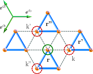
Figure 1: Triangular lattice: $\mathbf{r},\mathbf{r}^{\prime},\mathbf{r}^{\prime\prime}$ indicate the plaquettes involved in a given term of the Hamiltonian density. As an example, the sublattice “3” (inside the green circle) in the plaquette in $\mathbf{r}$ has three first neighbors “1” (each one inside a red dashed circle) indicated by labels k, k’ and k”. In top-left is shown the bond directors vectors.

With the aim to obtain the continuous limit, it is more convenient to rewrite the previous Hamiltonian as a sum of plaquette Hamiltonians $\mathcal{H}=\sum_{\mathbf{r}}H_{\mathbf{r}}$, where $\mathbf{r}$ is the plaquette label. This procedure allows us to write the Hamiltonian density $H_{\mathbf{r}}$ in a symmetric way in terms of two indices $i,j$ which denote the sublattices “$i$” and “$j$” (that from now on will be called flavor index), and an index $(k)$ denoting which neighbor of the sublattice “$j$” we are consideringDombre and Read (1989) (see Fig. 1). The indices $i,j$ and $k$ run from 1 to 3. From now on the $\mathbf{r}$ dependence of $H_{\mathbf{r}}$ (and the terms included in $H_{\mathbf{r}}$) and in the spin variables $\mathbf{S}_{j}$ is suppressed to simplify the notation, i.e. $H_{\mathbf{r}}\to H$, $\mathbf{S}_{i}(\mathbf{r})\to\mathbf{S}_{i}$. The plaquette Hamiltonian density $H$ reads

$$H = H_{E}+H_{DM}+H_{z}$$

$$H_{E} = \frac{J}{6}\sum_{i}\sum_{j\neq i}\sum_{k}\mathbf{S}_{i}\cdot\mathbf{S}_{j}^{(k)}$$

$$H_{DM} = \frac{1}{6}\sum_{i}\sum_{j\neq i}\sum_{k}\mathbf{D}^{(k)}_{ij}.\left(\mathbf{S}_{i}\times\mathbf{S}^{(k)}_{j}\right)$$

$$H_{Z} = -\frac{1}{3}\sum_{i}\mathbf{B}\cdot\mathbf{S}_{i}.$$ (2)

Assuming that each spin flavor varies slowly, an approximation that holds both near the ferromagnetic and the antiferromagnetic order, we can describe the continuum limit of each spin flavor by a smooth field configuration. Under such an assumption we can expand the value of the spin field $\mathbf{S}_{j}^{(k)}$ at site $j$ around the position of the spin $\mathbf{S}_{i}$ as follows:

$$\mathbf{S}^{k}_{j} = \mathbf{S}_{j}+a\left[\mathbf{e}^{(k)}_{ij}.\nabla\right]\mathbf{S}_{j}+\frac{a^{2}}{2}\left[\mathbf{e}^{(k)}_{ij}.\nabla\right]^{2}\mathbf{S}_{j}+\mathcal{O}(a^{3})$$

(3)

where $a$ is the nearest-neighbor distance, $\mathbf{e}^{(k)}_{ij}=-\text{sgn}[P(ij)]\mathbf{e}^{(k)}$, where $P(ij)$ is the permutation $(123)\rightarrow(ijl)$, with $\mathbf{e}^{(1)}=(1,0)$, $\mathbf{e}^{(2)}=(-\frac{1}{2},\frac{\sqrt{3}}{2})$, $\mathbf{e}^{(3)}=(-\frac{1}{2},-\frac{\sqrt{3}}{2})$ the bond directors (see Figure 1).

Performing a gradient expansion the exchange Hamiltonian density up to second order in $a$ reads:

$$H_{E} = J\sum_{i}\sum_{j\neq i}\left(\frac{a^{2}}{8}\mathbf{S}_{i}\nabla^{2}\mathbf{S}_{j}-\frac{1}{2}\mathbf{S}_{i}\cdot\mathbf{S}_{j}\right)+\text{const.},$$ (4)

The next term in Eq. (2) corresponds to the DM Hamiltonian density $H_{DM}$. Let us define a cyclic DM vectors $\mathbf{D}^{(k)}_{ij}=D\,\;\mathbf{e}^{(k)}_{ij}$ as in Ref. 31. Using the gradient expansion (3), $H_{DM}$, up to second order in $a$, becomes:

$$H_{DM} = \frac{1}{6}\sum_{i}\sum_{j\neq i}\sum_{k}\Big{[}\mathbf{D}^{(k)}_{ij}.\left(\mathbf{S}_{i}\times\mathbf{S}_{j}\right)+a\,\mathbf{D}^{(k)}_{ij}.(\mathbf{S}_{i}\times(\mathbf{e}^{(k)}_{ij}.\nabla)\mathbf{S}_{j})+\frac{a^{2}}{2}\mathbf{D}^{(k)}_{ij}.(\mathbf{S}_{i}\times(\mathbf{e}^{(k)}_{ij}.\nabla)^{2}\mathbf{S}_{j})\Big{]}$$ (5)

The first term on the right side in (5) vanishes, because $\sum_{k}\mathbf{e}^{(k)}_{ij}=0$. Using the definitions of $\mathbf{D}^{(k)}_{ij}$ and $\mathbf{e}^{(k)}_{ij}$, the second term reads

$$\frac{a}{6}\sum_{i}\sum_{j\neq i}\sum_{k}\mathbf{D}^{(k)}_{ij}\cdot\left[\mathbf{S}_{i}\times(\mathbf{e}^{(k)}_{ij}\cdot\nabla)\mathbf{S}_{j}\right]$$

$$= -\frac{aD\,}{4}\sum_{i}\sum_{j\neq i}\mathbf{S}_{i}\cdot(\nabla\times\mathbf{S}_{j})$$

Finally, the last term in (5) vanishes due to the antisymmetry of the DM-coupling ($\mathbf{D}_{\mathbf{r}\mathbf{r}^{\prime}}\equiv-\mathbf{D}_{\mathbf{r}^{\prime}\mathbf{r}}$). Hence the complete DM Hamiltonian density reads:

$$H_{DM} = -\frac{aD\,}{4}\sum_{i}\sum_{j\neq i}\mathbf{S}_{i}\cdot(\nabla\times\mathbf{S}_{j})$$ (6)

Putting all the pieces together we can write the complete Hamiltonian density ($H$) for an antiferromagnetic triangular chiral magnet in the continuous limit as

$$H = J\sum_{i,j\neq i}\frac{1}{2}\mathbf{S}_{i}\cdot\mathbf{S}_{j}+\frac{a^{2}}{8}\mathbf{S}_{i}\nabla^{2}\mathbf{S}_{j}-\frac{aD\,}{4J}\mathbf{S}_{i}\cdot(\nabla\times\mathbf{S}_{j})$$ (7)

$$-\frac{1}{3}\sum_{i}\mathbf{B}\cdot\mathbf{S}_{i}$$

The equations of motion of the previous Hamiltonian are non-linear and fairly difficult to solve analytically. Instead we study the Hamiltonian density proposing different families of Ansätze. In order to gain some intuition on the possible expressions we rewrite (7) by introducing a non-independent variable $M=\sum_{i}\mathbf{S}_{i}$, the plaquette magnetization. After some trivial algebraic manipulations Eq. (7) can be recasted in the following form:

$$H = H_{M}+\sum_{i=1}^{3}H_{i}$$ (8)

$$H_{M} = \frac{J}{2}(\mathbf{M}^{2}-3)+a^{2}\frac{J}{8}\mathbf{M}\cdot\nabla^{2}\mathbf{M}-\frac{aD\,}{4}\mathbf{M}\cdot(\nabla\times\mathbf{M})$$

$$H_{i} = -a^{2}\frac{J}{8}\mathbf{S}_{i}\nabla^{2}\mathbf{S}_{i}+\frac{aD\,}{4}\mathbf{S}_{i}\cdot(\nabla\times\mathbf{S}_{i})-\frac{1}{3}\mathbf{B}\cdot\mathbf{S}_{i}.$$

Some remarks are in order: we notice that the Hamiltonian density has been separated in four pieces. The first piece corresponds to a Hamiltonian density $H_{M}$ for the plaquette magnetization, while the rest corresponds to three copies of the same Hamiltonian density $H_{i}$, one for each flavor. Each of these $H_{i}$ has exactly the form of the ferromagnetic non-linear sigma model studied by Han et al. (2010) for chiral magnets. This is a crucial observation that, together with the knowledge of the finite temperature phases of the system Rosales et al. (2015), motivate the Ansätze that we propose in the following section. We also call the attention to the derivative term in the magnetization density that, at first sight, seems to lead to an energy unbounded from below. This is just an artifact of the introduction of the non-independent variable $\mathbf{M}$. The Laplacian term in the magnetization density has its origin in the exchange interaction term

$$J \sum_{i}\sum_{j\neq i}\mathbf{S}_{i}\cdot\mathbf{S}_{j}$$

$$= \frac{J}{2}\left(\mathbf{M}^{2}-3\right)+a^{2}\frac{J}{8}\mathbf{M}\cdot\nabla^{2}\mathbf{M}-a^{2}\frac{J}{8}\sum_{i}\mathbf{S}_{i}\nabla^{2}\mathbf{S}_{i},$$

and since the left-hand side of Eq.(4) is bounded from below, the right-hand side should be so as well. This means that the eventual large contribution that could arise from the term $a^{2}\frac{J}{8}\mathbf{M}\cdot\nabla^{2}\mathbf{M}$ will be compensated by the term $-a^{2}\frac{J}{8}\sum_{i}\mathbf{S}_{i}\nabla^{2}\mathbf{S}_{i}$. Hence, the full Hamiltonian remains bounded from below, as the original Hamiltonian. In fact, as it will be explicitly described in the next section, the derivative terms of the magnetization on the solutions are orders of magnitude smaller than the rest of the terms that appear in the Hamiltonian density (Eq. 8)

III Ansätze and Effective Low Energy Hamiltonian

The possibility to rewrite the continuum Hamiltonian as a sum of flavour Hamiltonian densities ($H_{i}$) plus a plaquette magnetization contribution ($H_{M}$), allows for an intuitive analysis. We mentioned in Sec. II that flavour Hamiltonians are exactly the continuum model found by Bogdanov and collaborators for ferromagnetic chiral magnets Bogdanov and Yablonskii (1989); Bogdanov and Hubert (1994). In Han et al. (2010), the authors have shown that this Hamiltonian admits a non-trivial periodic magnetic texture known as skyrmion-lattice (SkX), i.e. (a periodic arrange of skyrmions). So, the presence of three independent $H_{i}$ Hamiltonians in the continuum limit strongly suggests the possibility of the same kind of non-trivial SkX solutions on each sublattice.

These three independent equivalent SkX solutions need to be arranged in such a way that their sum, $\mathbf{M}$, minimizes the corresponding magnetization Hamiltonian.

III.1 Skyrmion crystal Ansatz

The proposed approximate solution to one spin flavour Hamiltonian can be constructed as a superposition of three helical solutions with wave vectors $\mathbf{k}_{\mu}$ satisfying $\sum_{\mu}\mathbf{k}_{\mu}=\bf{0}$ ($\mu=1,2,3$) in the plane of the sample with relative angles of $2\pi/3$ Okubo et al. (2012). The approximate skyrmion lattice solution then reads:

$$\mathbf{n}_{SkX}(\mathbf{r}) = \frac{1}{n}I_{xy}\sum_{\mu}\sin{[\frac{2\pi}{T}\mathbf{k}_{\mu}\cdot\mathbf{r}+\theta_{\mu}]}\mathbf{e}_{xy,\mu}+(m_{z}+I_{z}\sum_{\mu}\cos{[\frac{2\pi}{T}\mathbf{k}_{\mu}\cdot\mathbf{r}+\theta_{\mu}]})\mathbf{e}_{z},$$ (10)

where $T$ is the period of each helix; $n$ fixes the appropriate normalization $|\mathbf{n}_{SkX}|=1$ which restricts the values of the amplitudes $I_{xy}$ (in-plane) and $I_{z}$ (perpendicular to the xy-plane) and the homogeneous contribution to the magnetization in the $z-$direction $m_{z}$. $\mathbf{e}_{xy,\mu}$ are arbitrary unit vectors lying on the xy-plane satisfying $\sum_{\mu}\mathbf{e}_{xy,\mu}=\bf{0}$, while the phases $\theta_{\mu}$ satisfy $\cos(\theta_{1}+\theta_{2}+\theta_{3})=-1$Okubo et al. (2012).

The helix period $T$, that becomes the skyrmion lattice parameter, can be determined as a function of $I_{xy},I_{z}$ and $m_{z}$ by energy scale analysis (see the Appendix A). Now, the proposed Ansatz for the full solution reads:

$$\mathbf{S}_{1}(\mathbf{r}) = \mathbf{n}_{SkX}(\mathbf{r}),\;\;\mathbf{S}_{2}(\mathbf{r})=\mathbf{n}_{SkX}(\mathbf{r}+{\bf T}_{1}),$$

$$\mathbf{S}_{3}(\mathbf{r}) = \mathbf{n}_{SkX}(\mathbf{r}+{\bf T}_{2}),$$ (11)

where ${\bf T}_{1},{\bf T}_{2}$ are arbitrary translations in the xy-plane.

III.2 Helical Ansätz

In the helical phase, the spin structure is a special case of the Ansatz (10) and consists of three interpenetrating spirals on each sublattice, as in Eq. (11), but with a single-$\mathbf{k}_{\mu_{0}}$ mode

$$\mathbf{n}_{H}(\mathbf{r}) = \frac{1}{n}I_{xy}\sin{[\frac{2\pi}{T}\mathbf{k}_{\mu_{0}}\cdot\mathbf{r}+\theta]}\mathbf{e}_{xy}+(m_{z}+I_{z}\cos{[\frac{2\pi}{T}\mathbf{k}_{\mu_{0}}\cdot\mathbf{r}+\theta]})\mathbf{e}_{z},$$ (12)

where again the constant $n$ fixes the normalization $|\mathbf{n}_{H}|=1$.

III.3 Uniform sublattice Ansatz

The magnetic phase diagram for the model defined by Eq. (1) with $D=0$ has been discussed in Gvozdikova et al. (2011); Seabra et al. (2011). At zero temperture and zero magnetic field the ground state is a planar configuration with spins arranged in a $120^{\circ}$ structure described by the wave vector $k=(4\pi/3,0)$. In a magnetic field the energy is minimized when the constraint

$$\mathbf{S}_{1}+\mathbf{S}_{2}+\mathbf{S}_{3}=\mathbf{B}/(3J),$$ (13)

is fulfilled on each plaquette. This constraint persists up to the saturation field $B=9J$, where the spins are fully polarized.

For $D\neq 0$ the previous discussion breaks down since the DM term stabilizes new configurations. However, it is worth noting that even for $D\neq 0$ there exist spin configurations in which the DM contribution cancels out. This is the case when the spin field on each sublattice is uniform. This is easily seen from our effective model, since the DM term contains derivatives of the spin fields. If one goes back to the microscopic model, one can show that the sum of the interactions (through DM) of a specific spin with its six neighbors is zero for the present choice of the $\mathbf{D}$ vectors. Thus, for this kind of configurations, which we call SU for “sublattice uniform” from now on, the constraint given by Eq. (13) is still valid, and this is an equilibrium state to be considered in the following discussion of the phase diagram.

The energy per plaquette of the states satisfying the constraint (13) is field dependent, independent of $D$ and is given by:

$$E_{SU}=-\frac{B^{2}}{18J}-J\frac{3}{2}.$$ (14)

Finally, at the saturation the energy per plaquette of the ferromagnetic state (for $B>9J$) is

$$E_{FM}=3J-B.$$ (15)

Now that we have described the Ansätze under which we will study the Hamiltonian, we are in the position to compare the values of the terms that include derivatives of $\mathbf{M}$, to the rest of the terms included in the Hamiltonian density (8).

First, let us analyze these terms in the Helix phase. In this case, the plaquette magnetization corresponds to a superposition of three helical waves, each one given by Eq. (12), separated (in space) by a translation in the direction of propagation. In the case where the distance between peaks is uniform (i.e. the phase difference of each cosine is $2\pi/3$) it is straightforward to see from the Ansatz (12) that $\mathbf{M}$ will show small spatial variations: $\mathbf{M}(\mathbf{r})\approx\mathbf{M}=\text{const.}$. For the SkX phase, a similar analysis drives to the same conclusion. These statements are confirmed by our numerical calculations performed for both Ansätze for different values of the coupling $D$ and as a function of $\mathbf{B}$. Our results show that the plaquette magnetization is almost constant leading to the conclusion that the contribution of the laplacian and curl terms in $H_{M}$, are two orders of magnitude smaller than the rest of the terms present in the Hamiltonian density (8) (see figure 2). To this purpose we compare the four contributions (with spatial derivatives) of the total energy, namely: $E_{nlsm}$, $E_{dm}$ , $E_{Mnlsm}$ and $E_{Mdm}$, where

$$E_{nlsm} = -a^{2}\frac{J}{8}\sum_{\mathbf{r}}\sum_{i}\mathbf{S}_{i}\nabla^{2}\mathbf{S}_{i}$$ (16)

$$E_{dm} = \frac{aD\,}{4}\sum_{\mathbf{r}}\sum_{i}\mathbf{S}_{i}\cdot(\nabla\times\mathbf{S}_{i})$$ (17)

$$E_{Mnlsm} = a^{2}\frac{J}{8}\sum_{\mathbf{r}}\mathbf{M}\cdot\nabla^{2}\mathbf{M}$$ (18)

$$E_{Mdm} = -\frac{aD\,}{4}\sum_{\mathbf{r}}\mathbf{M}\cdot(\nabla\times\mathbf{M})$$ (19)

In figure 2 we plot the ratios between the four terms (16)-(19) setting $E_{dm}$ as the scale, for the case $D/J=1/2$. We observe that in the HL and AF-SkX phases both $E_{Mnlsm}/E_{dm}$ as well as $E_{Mdm}/E_{dm}$ are neglegible in almost all the field range, except for two narrow windows around the transition fields where the value of these ratios are smaller than $5\times 10^{-2}$. In the homogeneous SU and FM phases all the terms with derivatives are zero. This behaviour is repeated in all the range that we have explored $D/J<1$, leading to the conclusion that the contributions of the laplacian and curl terms in $H_{M}$, are at least two orders of magnitude smaller than the rest of the terms present in the Hamiltonian.

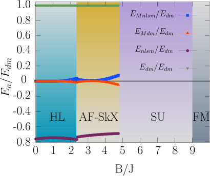
Figure 2: (Color online): Comparison between different contibutions from the density Hamiltonian (8) for the case $D/J=1/2$. We compare the four terms $E_{a}=\{E_{nlsm},E_{dm},E_{Mnlsm},E_{Mdm}\}$ (see Eqs. (16)-(19) ) using $E_{dm}$ as scale. In the HL and AF-SkX phases, the dominant terms are those coming from $\sum_{i}H_{i}$ in Eq. (8). All these terms are zero in the SU and FM (homogeneous) phases.

Monte Carlo simulations show that the spatial variation of the magnetization is small compared to the variation of the spin on each sublattice, confirming the observation made by the variational approach. Based on the previous analysis, we end up this section by proposing a simplified low-energy effective Hamiltonian that captures the low-energy physics of the antiferromagnetic chiral magnet given by Eq. (1).

III.4 Effective low energy theory

From the previous discussion we can rewrite Eq. (7) in the following form:

$$H = \sum_{i=1}^{3}H_{i}+H_{M}$$ (20)

$$H_{i} = -a^{2}\frac{J}{8}\mathbf{S}_{i}\nabla^{2}\mathbf{S}_{i}+\frac{aD\,}{4}\mathbf{S}_{i}\cdot(\nabla\times\mathbf{S}_{i})-\frac{1}{3}\mathbf{B}\cdot\mathbf{S}_{i}$$

$$H_{M} = \frac{J}{2}(\mathbf{M}^{2}-3).$$

It is remarkable that this continuum effective Hamiltonian can be thought as the sum of three Ginzburg-Landau (GL) effective actions (one for each flavor/sublattice) plus a term $H_{M}$ that couples them. From the first term of the sum one could expect, separately on each sublattice, the well known three phases, HL, SkX and FM.

IV Results and Phase Diagram

In this Section we construct the full phase diagram of the Hamiltonian (20), paying particular attention to the appearance of the topological AF-SkX phase.

In the study of the phase diagram we consider four phases, namely HL and SkX phases with energies $E_{HL}$ and $E_{SkX}$ respectively, together with SU and FM phases presented in section III. To find the minimum energy configuration we fix the variational parameters in an self consistent way by using the Nelder-Mead simplex method that is one of the most used for direct optimizationNelder and Mead (1965). The procedure consists of introducing an initial guess for $I_{xy}$ and $m_{z}$, and determine variationally the values of $\mathbf{T_{1}}$ and $\mathbf{T_{2}}$ self consistently.

The minimization of the variational energies for the different phases leads to the phase diagram shown in Fig. 3 (top) where the boundaries of the phases result from level crossings as shown in the Fig. 3 (bottom). As an example, in Fig. 4 we show a representative spin texture obtained by the variational Ansatz in the AF-SkX phase ($D/J=1/2$ and $B/J=3$).

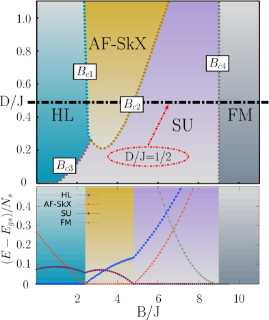
Figure 3: (Color online) Top: Phase diagram: dotted lines correspond to the boundaries between different phases labeled by the fiels $B_{c1}...B_{c4}$ (functions of $D$). Bottom: The energies ($E_{\text{phase}}-E_{\text{gs}}$) of the three states of triangular antiferromagnetic chiral magnet with $D/J=1/2$ as a function of the external magnetic field $B$. This example corresponds to the path indicated by the dashed black line in the phase diagram (Top).

The main features of this diagram is the presence of the four phases, namely HL, AF-SkX, SU and FM. in a wide region of $D-B$ ($D>0$) space. However, there exists a critical value $D_{c}\approx 0.2$ for the skyrmion lattice to be stable. Below this value, the skyrmion lattice phase is excluded irrespectively of the magnitude of the external field. The phase diagram for small fields is dominated by a helical phase with a wave vector lying in the plane. This phase starts at zero magnetic field $B=0$ and extends to $B_{c3}$ for $D<D_{c}$ and to $B_{c1}$ for $D>D_{c}$ (see Fig. 3).

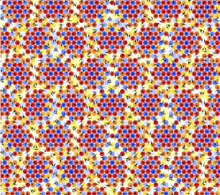
Figure 4: (Color online) Representative magnetic texture obtained by low energy effective theory (Eq. (20)) and the variational Ansätz for $D/J=1/2$ and $B/J=3$.

The phase diagram presents a wide region with a complex magnetic texture that is described by the superposition of three skyrmion lattices, one for each flavor. The region of the parameter space where this phase is stable is delimited by the curves $B_{c1}$ and $B_{c2}$. From $B_{c2}$ and $B_{c3}$ up to the saturation field $B_{c4}$ the SU phase is realized.

For the HL and AF-SkX phases, the optimized value of the period $T$ shows a small linear dependence in the external field (the same for both phases as obtained by MC simulationsRosales et al. (2015)). In Fig. 5 we see that the mean period takes the same values for the HL state and for AF-SkX state as $T(D)\simeq\frac{6.57}{D}-1.95$.

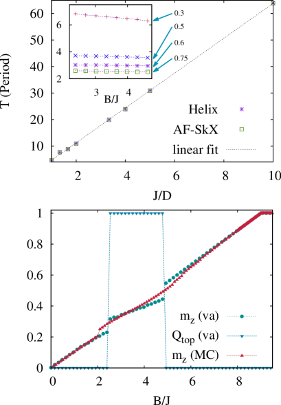
Figure 5: Top: Variation of the period with $J/D$ for SkX (green squares) and HL (purples stars). Inset: The skyrmion radius as a function of the external magnetic field for several values of $D$. Bottom: Topological charge $Q_{top}$ and magnetization $m^{T}_{z}$ as a function of the magnetic field for $D=0.5J$. (Bottom): Magnetization vs magnetic field $B$ calculated by variational Ansätz and by MC simulations.

For $D/J=1/2$, we get $T\approx 10.8\pm 0.6$ (this value should be compared with the wavelength $T\approx 11.4$ of the HL and AF-SkX phases found in Ref. 31 obtained by numerical simulations of finite-size systems). We can define the radius of a skyrmion (in one sub-lattice) as the radius of the circumference of the contour defined by $n_{z}=0$. In the inset of Fig. 5 (top) we show the skyrmion size as a function of the magnetic field. We observe that the behavior of the optimal skyrmion spacing as a function of the magnetic field varies very slowly in the region of the AF-SkX phase due to its topological stability. This behavior translates precisely in a wide range of stability of the AF-SkX phase in which the skyrmion number is fixed.

In order to capture the topological character of the field configuration for each spin flavor we introduce the topological index $Q_{top}$ and define the total (normalized) magnetization (z-component):

$$Q_{top} = \frac{1}{4\pi}\int_{u.c.}\mathbf{n}\cdot(\partial_{x}\mathbf{n}\times\partial_{y}\mathbf{n})\,d^{2}r,$$ (21)

$$m^{T}_{z} = \frac{1}{A_{u.c.}}\int_{u.c.}n_{z}\,d^{2}r,$$ (22)

where the integration is performed in a unit cell of the magnetic texture with area $A_{u.c.}$ (see Appendix A).

In Fig. 5 (bottom) we show the behavior of the magnetization and the topological charge as a function of the magnetic field. We see that the helical phase corresponds to a trivial configuration with $Q_{top}=0$ whereas in the SkX phase (triple-helix state) $Q_{top}=1$ because each unit cell contains only one skyrmion. The magnetization curve reveals an almost linear growth up to the saturation field. However, we see two discontinuities suggesting a first order phase transition form HL to AF-SkX phase and from AF-SkX to SU phase.

In order to confirm the results from the variational analysis, we numerically examine the ground state of the model (1) by Monte Carlo simulations based on the standard heatbath method combined with the over-relaxation method. We have implemented periodic boundary conditions for $N=3600$ sites. A run at each magnetic field or temperature contains typically $0.1-1\cdot 10^{6}$ Monte Carlo steps (MCS’s) for initial relaxation and twice MCS’s during the calculation of mean values. In Fig. 5 (bottom) we compare magnetization vs magnetic field for the minimized variational solution and by MC simulations for $D/J=1/2$. We observe qualitative agreement between both methods. However, the behaviour of the magnetization differs when the system switches from one phase to another. This may be due to finite size effects of the MC simulations and that in the transition region, the variational solution does not include higher order modes in ${\bf k}$. In Fig. 6 we compare the ground state energy as a function of the magnetic field obtained from the minimization of the variational energies for the different phases and by MC simulations for two values of $D/J$. The excellent agreement between both results further supports the variational analysis of the continuous limit of the microscopic Hamiltonian given by Eq. (20).

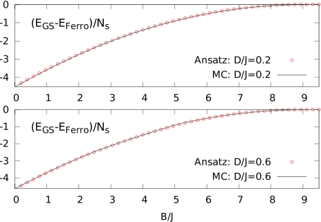
Figure 6: (Color online): Comparison of the energies vs magnetic field ($B$) obtained by variational Ansätz and MC simulations for $D/J=0.2$ and $0.6$. The specific values of $D/J$ were chosen as representative of two possible paths as a function of the external field $B$: one that goes directly from the HL phase to SU phase ($0.2$ case); and another in which the path goes through the AF-SkX phase ($0.6$).

V Discussion and Conclusion

To summarize, we have constructed a low-energy theory describing the behavior of the Heisenberg model in the triangular lattice including Dzyaloshinskii-Moriya interactions and the magnetic field. Our low energy effective theory given in Eq. (20), notwithstanding its simplicity, displays a plethora of phenomena of current interest in the context of topological magnetic phases. The effective theory obtained surprisingly consists of three independent Hamiltonian densities ($H_{i}$) similar to those found by Bogdanov et al.Bogdanov and Yablonskii (1989); Bogdanov and Hubert (1994) and Nagaosa et al.Han et al. (2010) in the context of ferromagnetic systems. Each one of these admit non-trivial magnetic structures known as skyrmion-lattices (SkX). In addition to these terms, there is a plaquette magnetization contribution ($H_{M}$) which couples the previous $H_{i}$’s. The low-energy theory predicts a AF-SkX crystal phase which consists of three interpenetrating SkX states as observed in numerical Monte Carlo simulationsRosales et al. (2015). The low-energy effective Hamiltonian reproduces the correct spin phenomenology and could serve as a first step to analyze the coupling to charge degrees of freedom. In addition we numerically examined the ground state of the micropcopic model by Monte Carlo simulations showing a very good agreement between both methods. Finally, the remarkable stability that presents the AF-SkX phase for a wide range of magnetic fields can have interesting consequences in the context of the anomalous Hall effect.

Appendix A Energy Scale Analysis

The magnetic textures considered in section III, namely helix and AF-SkX, are periodic configurations in $x$ and $y$ directions with periods $\alpha\,T$ and $\beta\,T$ respectively, with $\alpha,\beta$ to be fixed by the symmetry of the texture (for helix $\alpha=\beta=1$, and for AF-SkX $\alpha=1$ and $\beta=2/\sqrt{3}$). This allows to calculate the total energy as the energy of a cell (of area $A_{u.c.}=\alpha\beta T^{2}$) times the number of cells, $L^{2}/(\alpha\beta T^{2})$, in the sample. In addition, we separate different contributions in the energy density according to the order of spatial derivatives. With all this, the total energy can be written as

$$E(T,I_{xy},I_{z},m_{z})=\frac{L^{2}}{\alpha\beta T^{2}}\sum_{i=0}^{2}E_{i}(T,I_{xy},I_{z},m_{z}),$$ (23)

with

$$E_{i}(T,I_{xy},I_{z},m_{z}) = \int_{0}^{\alpha T}dx\int_{0}^{\beta T}dy\,\mathcal{E}_{i}(T,I_{xy},I_{z},m_{z}),$$

and $\mathcal{E}_{i}(T,I_{xy},I_{z},m_{z})$ denotes the energy density containing ith-order derivatives. We can rewrite the different terms using their properties under scale transformations ($\mathbf{r}\to\mathbf{r}^{\prime}=\mathbf{r}/T$). We can separate the dependence in $T$ as

$$E_{i}(T,I_{xy},I_{z},m_{z}) = \int_{0}^{\alpha T}dx\int_{0}^{\beta T}dy\,\mathcal{E}_{i}(T,I_{xy},I_{z},m_{z})$$

$$= T^{2-i}\int_{0}^{\alpha}dx^{\prime}\int_{0}^{\beta}dy^{\prime}\,\mathcal{E}_{i}(1,I_{xy},I_{z},m_{z})$$

$$= T^{2-i}E_{i}(1,I_{xy},I_{z},m_{z}),$$

and write the energy of the sample as

$$E(T,I_{xy},I_{z},m_{z})=\frac{L^{2}}{\alpha\beta}\left[\frac{E_{2}}{T^{2}}+\frac{E_{1}}{T}+E_{0}\right].$$

This shows that all the dependence in the variable $T$ can be cast as power law prefactors.

References

- Anderson (1987) P. W. Anderson, science 235, 1196 (1987).
- Mühlbauer et al. (2009) S. Mühlbauer, B. Binz, F. Jonietz, C. Pfleiderer, A. Rosch, A. Neubauer, R. Georgii, and P. Böni, Science 323, 915 (2009).
- Ishikawa et al. (1976) Y. Ishikawa, K. Tajima, D. Bloch, and M. Roth, Solid State Communications 19, 525 (1976).
- Ishikawa and Arai (1984) Y. Ishikawa and M. Arai, Journal of the Physical Society of Japan 53, 2726 (1984).
- Grigoriev et al. (2009) S. Grigoriev, V. Dyadkin, E. Moskvin, D. Lamago, T. Wolf, H. Eckerlebe, and S. Maleyev, Physical Review B 79, 144417 (2009).
- Lebech et al. (1995) B. Lebech, P. Harris, J. S. Pedersen, K. Mortensen, C. Gregory, N. Bernhoeft, M. Jermy, and S. Brown, Journal of magnetism and magnetic materials 140, 119 (1995).
- Pfleiderer et al. (2004) C. Pfleiderer, D. Reznik, L. Pintschovius, H. v. Löhneysen, M. Garst, and A. Rosch, Nature 427, 227 (2004).
- Janoschek et al. (2013) M. Janoschek, M. Garst, A. Bauer, P. Krautscheid, R. Georgii, P. Böni, and C. Pfleiderer, Physical Review B 87, 134407 (2013).
- Beille et al. (1983) J. Beille, J. Voiron, and M. Roth, Solid state communications 47, 399 (1983).
- Grigoriev et al. (2007) S. Grigoriev, V. Dyadkin, D. Menzel, J. Schoenes, Y. O. Chetverikov, A. Okorokov, H. Eckerlebe, and S. Maleyev, Physical Review B 76, 224424 (2007).
- Onose et al. (2005) Y. Onose, N. Takeshita, C. Terakura, H. Takagi, and Y. Tokura, Physical Review B 72, 224431 (2005).
- Lebech et al. (1989) B. Lebech, J. Bernhard, and T. Freltoft, Journal of Physics: Condensed Matter 1, 6105 (1989).
- Uchida et al. (2008) M. Uchida, N. Nagaosa, J. He, Y. Kaneko, S. Iguchi, Y. Matsui, and Y. Tokura, Physical Review B 77, 184402 (2008).
- Yu et al. (2011) X. Yu, N. Kanazawa, Y. Onose, K. Kimoto, W. Zhang, S. Ishiwata, Y. Matsui, and Y. Tokura, Nature materials 10, 106 (2011).
- Wilhelm et al. (2011) H. Wilhelm, M. Baenitz, M. Schmidt, U. Rößler, A. Leonov, and A. Bogdanov, Physical review letters 107, 127203 (2011).
- Shibata et al. (2013) K. Shibata, X. Yu, T. Hara, D. Morikawa, N. Kanazawa, K. Kimoto, S. Ishiwata, Y. Matsui, and Y. Tokura, Nature nanotechnology 8, 723 (2013).
- Skyrme (1962) T. H. R. Skyrme, Nuclear Physics 31, 556 (1962).
- Wright and Mermin (1989) D. C. Wright and N. D. Mermin, Reviews of Modern physics 61, 385 (1989).
- Sondhi et al. (1993) S. Sondhi, A. Karlhede, S. Kivelson, and E. Rezayi, Physical Review B 47, 16419 (1993).
- Ho (1998) T.-L. Ho, Physical Review Letters 81, 742 (1998).
- Sampaio et al. (2013) J. Sampaio, V. Cros, S. Rohart, A. Thiaville, and A. Fert, Nature nanotechnology 8, 839 (2013).
- Tomasello et al. (2014) R. Tomasello, E. Martinez, R. Zivieri, L. Torres, M. Carpentieri, and G. Finocchio, Scientific reports 4 (2014).
- Schwarze et al. (2015) T. Schwarze, J. Waizner, M. Garst, A. Bauer, I. Stasinopoulos, H. Berger, C. Pfleiderer, and D. Grundler, Nature materials (2015).
- Dzyaloshinsky (1958) I. Dzyaloshinsky, Journal of Physics and Chemistry of Solids 4, 241 (1958).
- Moriya (1960) T. Moriya, Physical Review Letters 4, 228 (1960).
- Bogdanov and Yablonskii (1989) A. Bogdanov and D. Yablonskii, Zh. Eksp. Teor. Fiz 95, 182 (1989).
- Bogdanov and Hubert (1994) A. Bogdanov and A. Hubert, Journal of magnetism and magnetic materials 138, 255 (1994).
- Rößler et al. (2006) U. Rößler, A. Bogdanov, and C. Pfleiderer, Nature 442, 797 (2006).
- Do Yi et al. (2009) S. Do Yi, S. Onoda, N. Nagaosa, and J. H. Han, Physical Review B 80, 054416 (2009).
- Han et al. (2010) J. H. Han, J. Zang, Z. Yang, J.-H. Park, and N. Nagaosa, Physical Review B 82, 094429 (2010).
- Rosales et al. (2015) H. D. Rosales, D. C. Cabra, and P. Pujol, Phys. Rev. B 92, 214439 (2015).
- Zang et al. (2011) J. Zang, M. Mostovoy, J. H. Han, and N. Nagaosa, Phys. Rev. Lett. 107 (2011).
- Dombre and Read (1989) T. Dombre and N. Read, Physical Review B 39, 6797 (1989).
- Okubo et al. (2012) T. Okubo, S. Chung, and H. Kawamura, Physical Review Letters 108, 017206 (2012).
- Gvozdikova et al. (2011) M. V. Gvozdikova, P.-E. Melchy, and M. E. Zhitomirsky, Journal of Physics: Condensed Matter 23, 164209 (2011).
- Seabra et al. (2011) L. Seabra, T. Momoi, P. Sindzingre, and N. Shannon, Phys. Rev. B 84, 214418 (2011).
- Nelder and Mead (1965) J. A. Nelder and R. Mead, The Computer Journal 7, 308 (1965).