Critical exponents for long-range $O(n)$
models below the upper critical dimension

Abstract

We consider the critical behaviour of long-range $O(n)$ models ($n\geq 0$) on ${{{\mathbb{Z}}}^{d}}$, with interaction that decays with distance $r$ as $r^{-(d+\alpha)}$, for $\alpha\in(0,2)$. For $n\geq 1$, we study the $n$-component $|\varphi|^{4}$ lattice spin model. For $n=0$, we study the weakly self-avoiding walk via an exact representation as a supersymmetric spin model. These models have upper critical dimension $d_{c}=2\alpha$. For dimensions $d=1,2,3$ and small $\epsilon>0$, we choose $\alpha=\frac{1}{2}(d+\epsilon)$, so that $d=d_{c}-\epsilon$ is below the upper critical dimension. For small $\epsilon$ and weak coupling, to order $\epsilon$ we prove existence of and compute the values of the critical exponent $\gamma$ for the susceptibility (for $n\geq 0$) and the critical exponent $\alpha_{H}$ for the specific heat (for $n\geq 1$). For the susceptibility, $\gamma=1+\frac{n+2}{n+8}\frac{\epsilon}{\alpha}+O(\epsilon^{2})$, and a similar result is proved for the specific heat. Expansion in $\epsilon$ for such long-range models was first carried out in the physics literature in 1972. Our proof adapts and applies a rigorous renormalisation group method developed in previous papers with Bauerschmidt and Brydges for the nearest-neighbour models in the critical dimension $d=4$, and is based on the construction of a non-Gaussian renormalisation group fixed point. Some aspects of the method simplify below the upper critical dimension, while some require different treatment, and new ideas and techniques with potential future application are introduced.

1 Introduction and main results

1.1 Introduction

The understanding of critical phenomena via the renormalisation group is one of the great achievements of physics in the twentieth century, as it simultaneously provides an explanation of universality, as well as a systematic method for the computation of universal quantities such as critical exponents. It remains a challenge to place these methods on a firm mathematical foundation.

For short-range Ising or $n$-component $|\varphi|^{4}$ spin systems ($n\geq 1$), the upper critical dimension is $d_{c}=4$, meaning that mean-field theory applies in dimensions $d>4$. Renormalisation group methods have been applied in a mathematically rigorous manner to study the critical behaviour of the $|\varphi|^{4}$ model in the upper critical dimension $d=4$, using block spin renormalisation in [50, 51, 57, 60] (for $n=1$), phase space expansion methods in [44] (for $n=1$), and using the methods that we apply and further develop in this paper in [13, 86, 18] (for $n\geq 1$). The low-temperature phase has been studied, e.g., in [8, 10]. For $n=0$, a supersymmetric version of the $|\varphi|^{4}$ model corresponds exactly to the weakly self-avoiding walk, and has been analysed in detail for $d=4$ [15, 14, 86, 18]. A model related to the 4-dimensional weakly self-avoiding walk is studied in [64]. Renormalisation group methods have recently been applied to gradient field models in [4], to the Coloumb gas in [43], to interacting dimers in [52], and to symmetry breaking in low temperature many-boson systems in [9]. For hierarchical models, the critical behaviour of spin systems was studied in [42, 48, 49, 58], and for weakly self-avoiding walk in [25, 29, 30]. An introductory account of a renormalisation group analysis of the 4-dimensional hierarchical $|\varphi|^{4}$ model, using methods closely related to those used in the present paper, is given in [12].

In a 1972 paper entitled “Critical exponents in 3.99 dimensions” [89], Wilson and Fisher explained how to apply the renormalisation group method in dimension $d=4-\epsilon$ for small $\epsilon>0$. This has long been physics textbook material, e.g., in [7, p.236] the values of the critical exponents for the susceptibility ($\gamma$), the specific heat ($\alpha_{H}$), the correlation length ($\nu$), and the critical two-point function ($\eta$) can be found:

$$\gamma =1+\frac{n+2}{n+8}\frac{\epsilon}{2}+\cdots,\quad\alpha_{H}=\frac{4-n}{n+8}\frac{\epsilon}{2}+\cdots,$$ (1.1)

$$\nu =\frac{1}{2}+\frac{n+2}{n+8}\frac{\epsilon}{4}+\cdots,\quad\eta=\frac{n+2}{(n+8)^{2}}\frac{\epsilon^{2}}{2}+\cdots.$$ (1.2)

Quadratic terms in $\epsilon$ are also given in [7], and terms up to order $\epsilon^{6}$ are known in the physics literature [69, 55, 66]. These $\epsilon$-expansions are believed to be asymptotic, but they must be divergent since analyticity at $\epsilon=0$ would be inconsistent with mean-field exponents for $\epsilon<0$ (which obey (1.1)–(1.2) with $\epsilon=0$). Critical exponents for dimension $d=3$ (corresponding to $\epsilon=4-d=1$) have been computed from the $\epsilon$ expansions via Borel resummation, and the results are consistent with those obtained via other methods [69, 55, 66].

The $\epsilon$ expansion is not mathematically rigorous—in particular the spin models are not directly defined in non-integer dimensions. This particular issue can be circumvented by considering long-range models with interaction decaying with distance as $|x|^{-(d+\alpha)}$, for $\alpha\in(0,2)$. It is known that these models have upper critical dimension $d_{c}=2\alpha$ [46, 6]; this is the dimension above which the bubble diagram converges (see Section 2.1.3). A hint that the long-range model may have an upper critical dimension that is lower than its short-range counterpart can be seen already from the fact that random walk on ${{{\mathbb{Z}}}^{d}}$ with step distribution decaying as $|x|^{-(d+\alpha)}$ is transient if and only if $d>\alpha$, as opposed to $d>2$ in the short-range case. That the upper critical dimension should be $2\alpha$ can be anticipated from the fact that the range of an $\alpha$-stable process has dimension $\alpha$ [22], so two independent processes generically do not intersect in dimensions above $2\alpha$. Several mathematical papers establish mean-field behaviour for long-range models in dimensions $d>d_{c}=2\alpha$, including [6, 62, 61, 39, 40, 41].

In a 1972 paper, Fisher, Ma and Nickel [46] carried out the $\epsilon$ expansion to compute critical exponents for long-range $O(n)$ models in dimension $d=d_{c}-\epsilon=2\alpha-\epsilon$; see also [83]. The work of Suzuki, Yamazaki and Igarashi [88] is roughly contemporaneous with that of Fisher, Ma and Nickel, and reaches similar conclusions. The results of [46, 88], which are not mathematically rigorous, include (see [46, (5),(9)])

$$\gamma =1+\frac{n+2}{n+8}\frac{\epsilon}{\alpha}+\cdots,\quad\eta=2-\alpha,$$ (1.3)

where we omit terms of order $\epsilon^{2}$ present in [46, 88]. If we assume the scaling relations $\gamma=(2-\eta)\nu$ and hyperscaling relation $\alpha_{H}=2-d\nu$, then we obtain

$$\nu =\frac{\gamma}{\alpha},\quad\alpha_{H}=\frac{4-n}{n+8}\frac{\epsilon}{\alpha}+\cdots.$$ (1.4)

Interestingly, the critical exponent $\eta$ was predicted to “stick” at the mean-field value $\eta=2-\alpha$ to all orders in $\epsilon$ [46, 83] (we are interested here only in $d=1,2,3$ and small $\epsilon$ and not in the range corresponding to crossover to short-range behaviour [63, 19, 23]). This has been proved very recently [71] for all $n\geq 0$, using an extension of the methods we develop here. Earlier, a proof that $\eta=2-\alpha$ for small $\epsilon$ was announced by Mitter for a 1-component continuum model [76]. The long-range model has also recently been studied in connection with conformal invariance of the critical theory for $d=d_{c}-\epsilon$ with $\epsilon$ small [2, 82].

From a mathematical point of view, the long-range $O(n)$ model has the advantage that it can be defined in integer dimension $d$ with $\alpha=\frac{1}{2}(d+\epsilon)$ chosen so that $d$ is just slightly below the upper critical dimension: $d=d_{c}-\epsilon=2\alpha-\epsilon$. This approach has been adopted in the mathematical physics literature [32, 79, 1], where the emphasis has been on the construction of a non-Gaussian renormalisation group fixed point, including a construction of a renormalisation group trajectory between the Gaussian and non-Gaussian fixed points in [1]. An earlier paper in a related direction is [24]. The papers [24, 32, 1] consider continuum models, whereas [79] considers a supersymmetric model on ${\mathbb{Z}}^{3}$ that is essentially the same as the $n=0$ model we consider here. None of these papers address the computation of critical exponents. Critical correlation functions were studied in a hierarchical version of the model in [48, 49], and the recent paper [3] carries out a computation of critical exponents in a different hierarchical setting; see also [2].

In this paper, we apply a rigorous renormalisation group method to the long-range $O(n)$ model on ${{{\mathbb{Z}}}^{d}}$, for $d=1,2,3$. To order $\epsilon$, we prove the existence of and compute the values of the critical exponent $\gamma$ for the susceptibility (for all $n\geq 0$) and the exponent $\alpha_{H}$ for the specific heat (for all $n\geq 1$). The case $n=0$ is treated exactly as a supersymmetric version of the $|\varphi|^{4}$ model, with most of the analysis carried out simultaneously and in a unified manner for the spin model ($n\geq 1$) and the weakly self-avoiding walk ($n=0$). This unification has grown out of work on the 4-dimensional case in [15, 13, 86, 18].

The proof adapts and applies a rigorous renormalisation group method that was developed in a series of papers with Bauerschmidt and Brydges for the nearest-neighbour models in the critical dimension $d=4$. Some aspects of the method require extension to deal with the fact that the renormalisation group fixed point is non-Gaussian for $d=d_{c}-\epsilon=2\alpha-\epsilon$. On the other hand, some aspects of the method simplify significantly compared to the critical dimension. We also adapt and simplify some ideas from the construction of the non-Gaussian fixed point in [32, 79]. We use the term “fixed point” loosely in this paper, as the notion itself is faulty here because the renormalisation group map does not act autonomously due to lattice effects. Nevertheless, our analysis is based on what would be a fixed point if the lattice effects were absent, and we persist in using the terminology.

The $|\varphi|^{4}$ model has been studied in the mathematical literature for many decades [53]. Recently its dynamical version and the connection with renormalisation and stochastic partial differential equations have received renewed interest [56, 67]. Our topic here is the equilibrium setting of the model, and we do not consider dynamics.

1.2 The $|\varphi|^{4}$ model

We now give a precise definition of the long-range $n$-component $|\varphi|^{4}$ model, for $n\geq 1$. As usual, it is defined first in finite volume, followed by an infinite volume limit.

Let $L,N>1$ be integers, and let $\Lambda=\Lambda_{N}={\mathbb{Z}}^{d}/L^{N}{\mathbb{Z}}^{d}$ be the $d$-dimensional discrete torus of side length $L^{N}$. Let $n\geq 1$. The spin field $\varphi$ is a function $\varphi:\Lambda\rightarrow{\mathbb{R}}^{n}$, denoted $x\mapsto\varphi_{x}$, and we sometimes write $\varphi\in({\mathbb{R}}^{n})^{\Lambda}$. The Euclidean norm of $v=(v^{1},\ldots,v^{n})\in{\mathbb{R}}^{n}$ is $|v|=[\sum_{i=1}^{n}(v^{i})^{2}]^{1/2}$, with inner product $v\cdot w=\sum_{i=1}^{n}v^{i}w^{i}$.

We fix a $\Lambda\times\Lambda$ real symmetric matrix $M$, and for $x\in\Lambda$ we define $(M\varphi)_{x}\in{\mathbb{R}}^{n}$ by the component-wise action $(M\varphi)_{x}^{i}=\sum_{y\in\Lambda}M_{xy}\varphi^{i}_{y}$. Given $g>0$ and $\nu\in{\mathbb{R}}$, we define a function $V:({\mathbb{R}}^{n})^{\Lambda}\rightarrow{\mathbb{R}}$ by

$$V(\varphi)=\sum_{x\in\Lambda}\big{(}\tfrac{1}{4}g|\varphi_{x}|^{4}+\textstyle{\frac{1}{2}}\nu|\varphi_{x}|^{2}+\textstyle{\frac{1}{2}}\varphi_{x}\cdot(M\varphi)_{x}\big{)}.$$ (1.5)

By definition, the quartic term is $|\varphi_{x}|^{4}=(\varphi_{x}\cdot\varphi_{x})^{2}$. The partition function is defined by

$$Z_{g,\nu,N}=\int_{({\mathbb{R}}^{n})^{\Lambda}}e^{-V(\varphi)}d\varphi,$$ (1.6)

where $d\varphi$ is the Lebesgue measure on $({\mathbb{R}}^{n})^{\Lambda}$. The expectation of a random variable $F:({\mathbb{R}}^{n})^{\Lambda}\rightarrow{\mathbb{R}}$ is

$$\langle F\rangle_{g,\nu,N}=\frac{1}{Z_{g,\nu,N}}\int_{({\mathbb{R}}^{n})^{\Lambda}}F(\varphi)e^{-V(\varphi)}d\varphi.$$ (1.7)

Thus $\varphi$ is a classical continuous unbounded $n$-component spin field on the torus $\Lambda$, i.e., with periodic boundary conditions.

For $f:{{{\mathbb{Z}}}^{d}}\rightarrow{\mathbb{R}}$ and $e\in{\mathbb{Z}}^{d}$ with $|e|_{1}=1$, the discrete gradient is defined by $(\nabla^{e}f)_{x}=f_{x+e}-f_{x}$. The gradient acts component-wise on $\varphi$, and has a natural interpretation for functions $f:\Lambda\rightarrow{\mathbb{R}}$. The discrete Laplacian is $\Delta=-\frac{1}{2}\sum_{e\in{\mathbb{Z}}^{d}:|e|_{1}=1}\nabla^{-e}\nabla^{e}$. The Laplacian has versions on both ${{{\mathbb{Z}}}^{d}}$ and the torus $\Lambda$, which we distinguish when necessary by writing $\Delta_{{{{\mathbb{Z}}}^{d}}}$ or $\Delta_{\Lambda}$. Let $\alpha\in(0,2)$. We choose $M$ to be the lattice fractional Laplacian $M=(-\Delta_{\Lambda})^{\alpha/2}$. Then (1.5) becomes

$$V(\varphi)=\sum_{x\in\Lambda}\Big{(}\tfrac{1}{4}g|\varphi_{x}|^{4}+\textstyle{\frac{1}{2}}\nu|\varphi_{x}|^{2}+\textstyle{\frac{1}{2}}\varphi_{x}\cdot((-\Delta_{\Lambda})^{\alpha/2}\varphi_{x})\Big{)}.$$ (1.8)

The definition and properties of the positive semi-definite operator $(-\Delta_{\Lambda})^{\alpha/2}$ are discussed in Section 2.1. Since $(-\Delta_{\Lambda})^{\alpha/2}_{x,y}\leq 0$ for $x\neq y$, $V$ is a ferromagnetic interaction which prefers spins to align. It is long-range, and on ${{{\mathbb{Z}}}^{d}}$ decays at large distance as $-(-\Delta_{{{{\mathbb{Z}}}^{d}}})^{\alpha/2}_{xy}\asymp|x-y|^{-(d+\alpha)}$. Here, and in the following, we write $a\asymp b$ to denote the existence of $c>0$ such that $c^{-1}b\leq a\leq cb$.

The susceptibility is defined by

$$\chi(g,\nu;n)=\lim_{N\rightarrow\infty}\sum_{x\in\Lambda_{N}}\langle\varphi_{0}^{1}\varphi_{x}^{1}\rangle_{g,\nu,N}=n^{-1}\lim_{N\rightarrow\infty}\sum_{x\in\Lambda_{N}}\langle\varphi_{0}\cdot\varphi_{x}\rangle_{g,\nu,N},$$ (1.9)

assuming the limit exists. We prove the existence of the infinite volume limit directly, with periodic boundary conditions and large $L$, in the situations covered by our theorems. The general theory of such infinite volume limits is well developed for $n=1,2$, but not for $n>2$ [45]. Even monotonicity of $\chi$ in $\nu$ is not known for all $n$, but it is to be expected that $\chi$ is monotone decreasing in $\nu$ and that there is a critical value $\nu_{c}=\nu_{c}(g;n)<0$ (depending also on $d$) such that $\chi(g,\nu;n)\uparrow\infty$ as $\nu\downarrow\nu_{c}$. We are interested in the nature of this divergence. For $g=0$, (1.8) is quadratic, (1.7) is a Gaussian expectation, $\nu_{c}(0;n)=0$, and $\chi(0,\nu;n)=(\nu-\nu_{c})^{-1}$ for $\nu>\nu_{c}=0$ (cf. (2.1.2)).

The pressure is defined by

$$p(g,\nu) =\lim_{N\rightarrow\infty}\frac{1}{|\Lambda_{N}|}\log Z_{g,\nu,N},$$ (1.10)

and the specific heat is defined by

$$c_{H}(g,\nu)=\frac{\partial^{2}p}{\partial\nu^{2}}(g,\nu).$$ (1.11)

Assuming the second derivative exists and commutes with the infinite volume limit,

$$\frac{\partial^{2}p}{\partial\nu^{2}}(g,\nu) =\lim_{N\rightarrow\infty}\tfrac{1}{4}\sum_{x\in\Lambda_{N}}\langle|\varphi_{0}|^{2};|\varphi_{x}|^{2}\rangle_{g,\nu,N},$$ (1.12)

where we write $\langle A;B\rangle=\langle AB\rangle-\langle A\rangle\langle B\rangle$ for the covariance or truncated expectation of random variables $A,B$. We are interested in the behaviour of the specific heat as $\nu\downarrow\nu_{c}$. Similar to the susceptibility, we prove the existence of the relevant infinite volume limits directly in the situations covered by our theorems.

1.3 Weakly self-avoiding walk

A continuous-time Markov chain $X$ with state space ${{{\mathbb{Z}}}^{d}}$ can be defined via specification of a $Q$ matrix [80], namely a ${{{\mathbb{Z}}}^{d}}\times{{{\mathbb{Z}}}^{d}}$ matrix $(Q_{xy})$ with $Q_{xx}<0$, $Q_{xy}\geq 0$ for $x\neq y$, and $\sum_{y}Q_{xy}=0$. Such a Markov chain takes steps from $x$ at rate $-Q_{xx}$, and jumps to $y$ with probability $-\frac{Q_{xy}}{Q_{xx}}$. The matrix $Q$ is called the infinitesimal generator of the Markov chain, and, for $t\geq 0$,

$$P_{x}(X(t)=y)=E_{x}(\mathbbm{1}_{X(t)=y})=(e^{tQ})_{xy},$$ (1.13)

where the subscripts on $P_{x}$ and $E_{x}$ specify $X(0)=x$. Here $P$ is the probability measure associated with $X$, and $E$ is the corresponding expectation.

The Laplacian $\Delta_{{{{\mathbb{Z}}}^{d}}}$ is a $Q$ matrix and generates the familiar nearest-neighbour continuous-time simple random walk. We fix instead $Q=-(-\Delta_{{{{\mathbb{Z}}}^{d}}})^{\alpha/2}$ with $\alpha\in(0,2)$. In Section 2.2, we verify the standard fact that this is indeed a $Q$ matrix as defined above. The Markov chain with this generator takes long-range steps, with the probability of a step from $x$ to $y$ decaying like $|x-y|^{-(d+\alpha)}$. The Green function $(-Q^{-1})_{xy}$ is finite for $\alpha<d$, and decays at large distance as $|x-y|^{-(d-\alpha)}$. We define the finite positive number $\tau^{(\alpha)}$ as the diagonal of the Green function:

$$\tau^{(\alpha)}=(-Q^{-1})_{00}=((-\Delta_{{{{\mathbb{Z}}}^{d}}})^{\alpha/2})^{-1}_{00}.$$ (1.14)

The local time of $X$ at $x$ up to time $T$ is the random variable $L_{T}^{x}=\int_{0}^{T}\mathbbm{1}_{X(t)=x}\;dt$. The self-intersection local time up to time $T$ is the random variable

$$I_{T}=\sum_{x\in{\mathbb{Z}}^{d}}\big{(}L_{T}^{x}\big{)}^{2}=\int_{0}^{T}\!\!\int_{0}^{T}\mathbbm{1}_{X(t_{1})=X(t_{2})}\;dt_{1}\,dt_{2}.$$ (1.15)

Given $g>0$ and $\nu\in{\mathbb{R}}$, the continuous-time weakly self-avoiding walk susceptibility is defined by

$$\chi(g,\nu;0)=\int_{0}^{\infty}E_{0}(e^{-gI_{T}})e^{-\nu T}dT.$$ (1.16)

The name “weakly self-avoiding walk” arises from the fact that the factor $e^{-gI_{T}}$ serves to discount trajectories with large self-intersection local time. A standard subadditivity argument (a slight adaptation of [15, Lemma A.1]) shows that for all dimensions $d\geq 1$ there exists a $d$-dependent critical value $\nu_{c}=\nu_{c}(g;0)\in[-2g\tau^{(\alpha)},0]$ such that

$$\text{$\chi(g,\nu;0)<\infty$ \; if and only if \; $\nu>\nu_{c}$}.$$ (1.17)

We are interested in the nature of the divergence of $\chi$ as $\nu\downarrow\nu_{c}$.

Our notation above reflects the fact that the weakly self-avoiding walk corresponds to the $n=0$ case of the $n$-component $|\varphi|^{4}$ model. Our methods treat both cases $n\geq 1$ (spins) and $n=0$ (self-avoiding walk) simultaneously, by using a supersymmetric spin representation for the weakly self-avoiding walk. This aspect is reviewed in Section 11.

1.4 Main results

We consider dimensions $d=1,2,3$; fixed $\epsilon>0$ (small); and

$$\alpha=\textstyle{\frac{1}{2}}(d+\epsilon).$$ (1.18)

In particular, $\alpha$ lies in the interval $(0,2)$. The upper critical dimension is $d_{c}=2\alpha$, and $d=d_{c}-\epsilon$ is below the upper critical dimension. Our main results are given by the following two theorems, which provide statements consistent with the values of $\gamma,\alpha_{H}$ in (1.3)–(1.4). The first theorem applies to both the spin and self-avoiding walk models, whereas the second applies only to the spin models. In the statements of the theorems, and throughout their proofs, the order of choice of $L$ and $\epsilon$ is that first $L$ is chosen large, and then $\epsilon$ is chosen small depending on $L$.

Theorem 1.1.

Let $n\geq 0$, let $L$ be sufficiently large, and let $\epsilon>0$ be sufficiently small. There exists $\bar{s}\asymp\epsilon$ such that, for $g\in[\frac{63}{64}\bar{s},\frac{65}{64}\bar{s}]$, there exist $\nu_{c}=\nu_{c}(g;n)$ and $C>0$ such that for $\nu=\nu_{c}+t$ with $t\downarrow 0$,

$$C^{-1}t^{-(1+\frac{n+2}{n+8}\frac{\epsilon}{\alpha}-C\epsilon^{2})}\leq\chi(g,\nu;n)\leq Ct^{-(1+\frac{n+2}{n+8}\frac{\epsilon}{\alpha}+C\epsilon^{2})}.$$ (1.19)

This is a statement that the critical exponent $\gamma$ exists to order $\epsilon$, and

$$\gamma=1+\frac{n+2}{n+8}\frac{\epsilon}{\alpha}+O(\epsilon^{2}).$$ (1.20)

The critical point obeys (recall (1.14))

$$\nu_{c}(g;n)=-(n+2)\tau^{(\alpha)}g(1+O(g)).$$ (1.21)

Theorem 1.2.

Let $n\geq 1$, let $L$ be sufficiently large, and let $\epsilon>0$ be sufficiently small. For $g\in[\frac{63}{64}\bar{s},\frac{65}{64}\bar{s}]$, and for $\nu=\nu_{c}+t$ with $t\downarrow 0$,

$$c_{H}(g,\nu;n) \asymp t^{-\frac{4-n}{n+8}\frac{\epsilon}{\alpha}+O(\epsilon^{2})}\quad (n<4),$$

$$c_{H}(g,\nu;n) \leq O(t^{-O(\epsilon^{2})}) (n=4),$$ (1.22)

$$c_{H}(g,\nu;n) \asymp 1 (n>4).$$

More explicitly, for $n<4$, (1.2) is shorthand for the existence of $C>0$ such that

$$C^{-1}t^{-(\frac{4-n}{n+8}\frac{\epsilon}{\alpha}-C\epsilon^{2})}\leq c_{H}(g,\nu;n)\leq Ct^{-(\frac{4-n}{n+8}\frac{\epsilon}{\alpha}+C\epsilon^{2})}\quad(n<4).$$ (1.23)

This is a statement that the critical exponent $\alpha_{H}$ is

$$\alpha_{H}=\frac{4-n}{n+8}\frac{\epsilon}{\alpha}+O(\epsilon^{2})\quad(n<4),$$ (1.24)

whereas the specific heat is at most $Ct^{-C\epsilon^{2}}$ for $n=4$ and is not divergent for $n>4$.

Mean-field behaviour has been proved for $d>4$ for the nearest-neighbour $\varphi^{4}$ model [5, 47, 84, 45, 87] (e.g., $\gamma=1$, $\alpha_{H}=0$), and for the nearest-neighbour strictly self-avoiding walk [38, 59]. For long-range self-avoiding walk (spread-out via a small parameter) in dimensions $d>2\alpha$, it has been proved that $\gamma=1$, that the scaling limit is an $\alpha$-stable process, in addition to other results [61, 40]. For the nearest-neighbour model in dimension $d=d_{c}=4$, logarithmic corrections to mean-field scaling are proved in [15, 13, 18, 86]; the first such result was obtained for the case $n=1$ in [60]. In contrast, Theorems 1.1–1.2 study critical behaviour below the upper critical dimension.

1.5 Organisation

The proof of Theorems 1.1–1.2 involves several components, some of which are closely related to components used to analyse the nearest-neighbour model in dimension 4 [15, 13], and some of which are new or are adaptations of methods of [32, 79]. We now describe the organisation of the paper, and comment on aspects of the proof.

We begin in Section 2 with a review of elementary facts about the fractional Laplacian, both on ${{{\mathbb{Z}}}^{d}}$ and on the torus $\Lambda_{N}$. The renormalisation group method we apply is based on a finite-range decomposition of the resolvent of the fractional Laplacian. Such a decomposition was recently provided in [77], and in Section 3 we introduce the aspects we need. Some detailed proofs of results needed for the finite-range decomposition are deferred to Section 10, where in particular an ingredient in [77] is corrected.

The finite-range decomposition allows expectations such as (1.7) to be evaluated progressively, in a multi-scale analysis. This is described in Section 4, where the first aspects of the renormalisation group method are explained. We concentrate our exposition on the case $n\geq 1$, as the case $n=0$ can be handled via minor notational changes using the supersymmetric representation of the weakly self-avoiding walk outlined in Section 11. In Section 4, we note a major simplification here compared to the nearest-neighbour model for $d=4$: the monomial $|\nabla\varphi|^{2}$ is irrelevant for the renormalisation group flow. This means that the coupling constants $z_{j},y_{j}$ used in [15, 13] are unnecessary, and that there is no need to tune the wave function renormalisation $z_{0}$. Also, the monomial $|\varphi|^{4}$ is relevant for the renormalisation group flow in our current setting, whereas it was marginal for $d=4$. This requires changes to the analysis for $d=4$.

In Section 5, we develop perturbation theory and state the second-order perturbative flow equations; these can be taken from [13]. We also state estimates on the coefficients appearing in those flow equations, and defer proofs of these estimates to Section 10. We identify the perturbative value of the nonzero fixed point $\bar{s}$ for the flow of the coupling constant $g_{j}$ for $|\varphi|^{4}$. This $\bar{s}$ is the number appearing in the statements of Theorems 1.1–1.2. As in [1, 32, 79], we must study the deviation of the flow of the coupling constant $g_{j}$ (coefficient of $|\varphi|^{4}$) from the fixed point. This is a feature that differs from $d=4$, where the fixed point is the Gaussian one and the analogue of $\bar{s}$ is $0$.

In Section 6, we recall aspects of the nonperturbative renormalisation group analysis applied in [15, 13]. We apply the main result of [37] to handle the nonperturbative analysis, with adaptation to take into account the new scaling in our present setting. The norms we use simplify compared to [13, 15], because it is no longer necessary to include the running coupling constant $g_{j}$ as a norm parameter. This was a serious technical difficulty for $d=4$ because in that case $g_{j}\rightarrow 0$. Our treatment of scales beyond the so-called mass scale differs from that in [15, 13] and is inspired by, but is not identical to, the treatment in [18].

In Section 7, we analyse the dynamical system arising from the renormalisation group. Our analysis is inspired in part by the corresponding analysis in [24, 32, 79], but it is done differently and in some aspects more simply, and it must account for the fact that we work slightly away from the critical point unlike in those references. A simplification compared to $d=4$ is that the dynamical system is hyperbolic, rather than non-hyperbolic as in [17]. On the other hand, the flow now converges to a non-Gaussian fixed point. It is in Section 7 that we take the main step in identifying the critical point $\nu_{c}$. The methods of Section 7 constitute one of the main novelties in the paper.

We transfer the conclusions from Section 7 concerning the dynamical system to analyse the flow equations and use this analysis to prove Theorems 1.1–1.2 in Sections 8–9, respectively. The ideas in Sections 8–9 share many features with [13, 15], but here it is more delicate.

1.6 Discussion

1.6.1 Speculative extensions

In the following discussion, we use “$\approx$” to denote uncontrolled approximation in arguments whose rigorous justification is not within the current scope of the methods in this paper, but which nevertheless provide two interpretations of our main results.

Firstly, for $n=1,2,3$, consider the critical correlation function $\langle|\varphi_{0}|^{2};|\varphi_{x}|^{2}\rangle_{\nu_{c}}$. We argue now that Theorem 1.2 is consistent with

$$\langle|\varphi_{0}|^{2};|\varphi_{x}|^{2}\rangle_{\nu_{c}}\approx|x|^{-(d-\epsilon\frac{4-n}{n+8})}.$$ (1.25)

For $n=1$, this agrees with the scaling in [2, Conjecture 6], as the exponent $d-\frac{\epsilon}{3}$ is equal to $2[\varphi^{2}]$ with $[\varphi^{2}]=2[\varphi]+\frac{\epsilon}{3}$ and $[\varphi]=\frac{1}{2}(d-\alpha)$. To obtain (1.25), suppose that $\langle|\varphi_{0}|^{2};|\varphi_{x}|^{2}\rangle_{\nu_{c}}\approx|x|^{-d+q}$, with $q$ to be determined. Write $\nu_{t}=\nu_{c}+t$ with $t>0$, so $\nu_{t}>\nu_{c}$. Then, with $\xi_{t}=\xi(\nu_{t})$ the correlation length, we expect that

$$c_{H}(\nu_{t}) =\frac{1}{4}\sum_{x\in{{{\mathbb{Z}}}^{d}}}\langle|\varphi_{0}|^{2};|\varphi_{x}|^{2}\rangle_{\nu_{t}}\approx\sum_{|x|\leq\xi_{t}}\langle|\varphi_{0}|^{2};|\varphi_{x}|^{2}\rangle_{\nu_{t}}$$

$$\approx\sum_{|x|\leq\xi_{t}}\langle|\varphi_{0}|^{2};|\varphi_{x}|^{2}\rangle_{\nu_{c}}\approx\sum_{1\leq|x|\leq\xi_{t}}|x|^{-d+q}\approx\xi_{t}^{q}\approx t^{-\nu q}=t^{-\gamma q/\alpha},$$ (1.26)

where we inserted $\nu=\gamma/\alpha$ from (1.4) in the last step. This gives $\alpha_{H}=\gamma q/\alpha$. With the values of $\gamma$ and $\alpha_{H}$ from Theorems 1.2 and 1.1, this gives, as claimed above,

$$q=\frac{4-n}{n+8}\epsilon+O(\epsilon^{2})\quad(n=1,2,3).$$ (1.27)

Secondly, for $n=0$, assuming the applicability of Tauberian theory, Theorem 1.1 is consistent with

$$E_{0}(e^{-gI_{T}})\approx e^{\nu_{c}T}T^{\frac{1}{4}\frac{\epsilon}{\alpha}+O(\epsilon^{2})}.$$ (1.28)

In addition, assuming again that $\nu=\gamma/\alpha$, we expect the typical end-to-end distance of the weakly self-avoiding walk to be given, for $0<p<\alpha$, by

$$\left[\frac{E_{0}(|X(T)|^{p}e^{-gI_{T}})}{E_{0}(e^{-gI_{T}})}\right]^{1/p}\approx T^{\nu}=T^{\frac{1}{\alpha}(1+\frac{1}{4}\frac{\epsilon}{\alpha})+O(\epsilon^{2})}.$$ (1.29)

Also, assuming that (1.25) and (1.27) apply also to $n=0$ leads to the prediction that

$$\int_{0}^{\infty}\int_{0}^{\infty}E_{0}[e^{-gI_{2}(T_{1},T_{2})}\mathbbm{1}_{X^{1}(T_{1})=X^{2}(T_{2})=x}]e^{-\nu_{c}(T_{1}+T_{2})}dT_{1}dT_{2}\approx|x|^{-d+\frac{1}{2}\epsilon},$$ (1.30)

where $X^{1}$ and $X^{2}$ are independent Markov chains as in Section 1.3 and $I_{2}(T_{1},T_{2})=\sum_{x}(L_{T_{1}}^{x}(X_{1})+L_{T_{2}}^{x}(X_{2}))^{2}$. In [86], a detailed analysis of such critical “watermelon diagrams” and their relation to critical correlations of field powers like (1.25) is given for the nearest-neighbour case when $d=4$.

1.6.2 Open problems

It would be of interest to attempt to extend the methods applied here to the following problems:

1. Very recently the $|x|^{-(d-\alpha)}$ decay of the critical two-point function $\langle\varphi_{0}\cdot\varphi_{x}\rangle_{\nu_{c}}$ has been proved for $n\geq 1$, as well as for its $n=0$ counterpart [71]. This required the introduction of observables into the renormalisation group analysis presented here. It would be of interest to extend this to other critical correlation functions including $\langle|\varphi_{0}|^{2};|\varphi_{x}|^{2}\rangle_{\nu_{c}}$ discussed in (1.25), and also (1.30). Such quantities are analysed for $d=4$ in [14, 86].

   In [82], for $n=1$, it is argued that appropriately adapted critical correlations $\langle\varphi_{0};\varphi_{x}^{3}\rangle_{\nu_{c}}$ and $\langle\varphi_{0}^{2};\varphi_{x}^{4}\rangle_{\nu_{c}}$ vanish in the long-range model due to conformal invariance. These correlations go beyond what was studied in [86] for $d=4$, and the work of [82] provides additional motivation to investigate such matters rigorously.

2. Extend the methods of [18] to analyse the correlation length and confirm the scaling relation $\nu=\gamma/\alpha$. For the long-range model, there can be no exponential decay of correlations, so the correlation length should be studied in terms of $\xi_{p}$, the correlation length of order $p$ ($0<p<\alpha$), as in [18].

3. Study scaling limits of the spin field for $n\geq 1$. Work in this direction was initiated for the nearest-neighbour model with $d=4$ in [13], but for the long-range model with $\epsilon>0$ there will be non-Gaussian scaling limits.

4. Prove (1.28)–(1.29). This needs new ideas even for the nearest-neighbour model on ${\mathbb{Z}}^{4}$, but the difficulties have been overcome for the 4-dimensional hierarchical model [25, 29, 30].

5. Study the upper critical dimension, with $\alpha=\frac{d}{2}$, i.e., $\epsilon=0$, for $d=1,2,3$. The analysis should have much in common with that used in [15, 13] for the short-range model with $d=4$, with the simplification that wave function renormalisation will not be required (i.e., $z_{0}=0$).

2 Fractional Laplacian

The fractional Laplacian is a much-studied object [70], particularly in the continuum setting. Our focus is the discrete setting, and we review relevant aspects here for arbitrary $d\geq 1$ and $\alpha\in(0,2)$. We often write $\beta=\frac{\alpha}{2}\in(0,1)$.

2.1 Definition and basic properties

2.1.1 Definition of fractional Laplacian

Let $d\geq 1$. Let $J$ be the ${{{\mathbb{Z}}}^{d}}\times{{{\mathbb{Z}}}^{d}}$ matrix with $J_{xy}=1$ if $|x-y|_{1}=1$, and otherwise $J_{xy}=0$. Let $I$ denote the identity matrix. The lattice Laplacian on ${{{\mathbb{Z}}}^{d}}$, with our normalisation, is

$$\Delta=J-2dI.$$ (2.1)

There are various equivalent ways to define the ${{{\mathbb{Z}}}^{d}}\times{{{\mathbb{Z}}}^{d}}$ matrix $(-\Delta)^{\beta}_{x,y}$, as follows.

Fourier transform. The matrix element $-\Delta_{xy}$ can be written as a Fourier integral

$$-\Delta_{x,y}=\frac{1}{(2\pi)^{d}}\int_{[-\pi,\pi]^{d}}\lambda(k)e^{ik\cdot(x-y)}dk$$ (2.2)

with

$$\lambda(k)=4\sum_{j=1}^{d}\sin^{2}(k_{j}/2)=2\sum_{j=1}^{d}(1-\cos k_{j}).$$ (2.3)

The matrix $(-\Delta)^{\beta}$ is defined by

$$(-\Delta)^{\beta}_{x,y}=\frac{1}{(2\pi)^{d}}\int_{[-\pi,\pi]^{d}}\lambda(k)^{\beta}e^{ik\cdot(x-y)}dk.$$ (2.4)

Taylor expansion. Let $D=\frac{1}{2d}J$. Then

$$(-\Delta)^{\beta}=(2d)^{\beta}(I-D)^{\beta}=(2d)^{\beta}\sum_{n=0}^{\infty}(-1)^{n}\binom{\beta}{n}D^{n}.$$ (2.5)

The coefficient $(-1)^{n}\binom{\beta}{n}=\binom{n-1-\beta}{n}$ is negative for $n\geq 1$, and equals $1$ for $n=0$. By Stirling’s formula,

$$(-1)^{n}\binom{\beta}{n}\sim-\frac{\beta}{\Gamma(1-\beta)}\frac{1}{n^{1+\beta}}\quad\text{as $n\rightarrow\infty$}.$$ (2.6)

The matrix elements $(D^{n})_{x,y}$ are the $n$-step transition probabilities for discrete-time nearest-neighbour simple random walk on ${{{\mathbb{Z}}}^{d}}$.

Stable subordinator. Via the change of variables $s=u/t$, it is immediately seen (apart from the value of the constant) that

$$t^{\beta}=\frac{\beta}{\Gamma(1-\beta)}\int_{0}^{\infty}(1-e^{-st})s^{-1-\beta}ds.$$ (2.7)

This explicitly exhibits the Lévy measure $\frac{\beta}{\Gamma(1-\beta)}s^{-1-\beta}ds$ for the Laplace exponent of the stable subordinator, i.e., for the Bernstein function $t\mapsto t^{\beta}$ [85]. Now put $t=-\Delta$ to get [90, p.260 (5)]

$$(-\Delta)^{\beta}=\frac{\beta}{\Gamma(1-\beta)}\int_{0}^{\infty}(I-e^{s\Delta})s^{-1-\beta}ds.$$ (2.8)

A related formula [90, p.260 (4)] is

$$(-\Delta)^{\beta}=\frac{\sin\beta\pi}{\pi}\int_{0}^{\infty}(-\Delta+s)^{-1}(-\Delta)s^{-1+\beta}ds.$$ (2.9)

We do not make use of (2.8)–(2.9), though Proposition 2.3 below bears relation to (2.9).

The following lemma shows that $-(-\Delta)^{\beta}_{0,x}$ has $|x|^{-d-2\beta}$ decay ($|x|$ denotes the Euclidean norm $|x|_{2}$). A much more general result can be found in [21, Theorem 5.3], including an asymptotic formula with precise constant. We provide a simple proof based on an estimate for simple random walk. Let $D=\frac{1}{2d}J$ as above. For $n$ and $x$ of the same parity, with $0<|x|_{\infty}\leq n$, the heat kernel estimate

$$\frac{c}{n^{d/2}}e^{-|x|^{2}/cn}\leq(D^{n})_{0,x}\leq\frac{C}{n^{d/2}}e^{-|x|^{2}/Cn}$$ (2.10)

is proved in [54, Theorem 3.1]. Unlike standard local central limit theorems which give precise constants (e.g., [68]), (2.10) includes exponential upper and lower bounds for $x$ well beyond the diffusive scale, e.g., for $|x|\asymp n$.

Lemma 2.1.

For $d\geq 1$ and $\beta\in(0,1)$, as $|x|\rightarrow\infty$, $-(-\Delta)^{\beta}_{0,x}\asymp|x|^{-d-2\beta}$.

Proof.

By (2.5)–(2.6) and (2.10), it suffices to prove that

$$\sum_{n=|x|}^{\infty}\frac{1}{n^{1+\beta+d/2}}e^{-c|x|^{2}/n}\asymp\frac{1}{|x|^{d+2\beta}}.$$ (2.11)

For the lower bound of (2.11), we bound the left-hand side below by

$$e^{-c}\sum_{n=|x|^{2}}^{2|x|^{2}}\frac{1}{n^{1+\beta+d/2}} \geq c^{\prime}\frac{1}{|x|^{d+2\beta}}.$$ (2.12)

For the upper bound, we use (with change of variables $t=s|x|^{2}$)

$$\sum_{n=|x|}^{\infty}\frac{1}{n^{1+\beta+d/2}}e^{-c|x|^{2}/n} \leq C\int_{0}^{\infty}\frac{1}{t^{1+\beta+d/2}}e^{-c|x|^{2}/t}dt=\frac{1}{|x|^{d+2\beta}}C\int_{0}^{\infty}\frac{1}{s^{1+\beta+d/2}}e^{-c/s}ds.$$ (2.13)

The integral on the right-hand side is a positive constant, and this completes the proof.  

2.1.2 Resolvent of fractional Laplacian

For $m^{2}\geq 0$, the resolvent of $-\Delta$ is given by

$$(-\Delta+m^{2})_{0,x}^{-1} =\frac{1}{(2\pi)^{d}}\int_{[-\pi,\pi]^{d}}\frac{e^{ik\cdot x}}{\lambda(k)+m^{2}}dk.$$ (2.14)

The integral converges for $d\geq 1$ if $m^{2}>0$, and also for $m^{2}=0$ when $d>2$. The resolvent of $(-\Delta)^{\beta}$ is

$$((-\Delta)^{\beta}+m^{2})_{0,x}^{-1} =\frac{1}{(2\pi)^{d}}\int_{[-\pi,\pi]^{d}}\frac{e^{ik\cdot x}}{(\lambda(k))^{\beta}+m^{2}}dk,$$ (2.15)

where now convergence requires $d>2\beta$ if $m^{2}=0$. For the massless case, an asymptotic formula $((-\Delta)^{\beta})_{0x}^{-1}\sim a_{\beta}|x|^{-(d-2\beta)}$ is proven in [20, Theorem 2.4], with precise constant $a_{\beta}$. For $m^{2}>0$, an upper bound

$$((-\Delta)^{\beta}+m^{2})^{-1}_{0x}\leq c_{\beta}\frac{1}{|x|^{d-2\beta}}\frac{1}{1+m^{4}|x|^{4\beta}}$$ (2.16)

is proven in Lemma 3.2 below.

The next proposition is due to [65] (see also [90, p.260 (6)]), and was rediscovered in [77]. Because it plays an essential role in our analysis, we provide a simple direct proof based on the following lemma. For $\beta\in(0,1)$, $a\geq 0$ and $s>0$, let

$$\rho^{(\beta)}(s,a)=\frac{\sin\pi\beta}{\pi}\frac{s^{\beta}}{s^{2\beta}+a^{2}+2as^{\beta}\cos\pi\beta}.$$ (2.17)

An elementary proof that $\rho^{(\beta)}(s,a)\geq 0$ is given in [77, Proposition 2.1].

Lemma 2.2.

Let $\beta\in(0,1)$, $t\geq 0$ and $a\geq 0$, excepting $t=a=0$. Then

$$\frac{1}{t^{\beta}+a}=\int_{0}^{\infty}\frac{1}{s+t}\;\rho^{(\beta)}(s,a)ds.$$ (2.18)

Proof.

We first consider $t>0$ and $a\geq 0$. Let $C$ be a simple closed contour that encloses $t$ in the cut plane $\mathbb{C}\setminus(-\infty,0]$, oriented counterclockwise. We define $z^{\beta}$ to be the branch given by $z^{\beta}=r^{\beta}e^{i\beta\theta}$, for $z=re^{i\theta}$ with $\theta\in[-\pi,\pi)$. By the Cauchy integral formula,

$$\frac{1}{t^{\beta}+a}=\frac{1}{2\pi i}\oint_{C}\frac{1}{z-t}\frac{1}{z^{\beta}+a}dz,$$ (2.19)

since $z^{\beta}+a$ has no zero inside $C$ (for $a>0$ and $z=re^{i\theta}$, a zero requires $e^{i\theta\beta}=-1$ which cannot happen for $\beta\in(0,1)$ and $\theta\in[-\pi,\pi)$).

Now we deform the contour to a keyhole contour around the branch cut. We shrink the small circle at the origin, and send the big circle to infinity; the contributions from both circles vanish in the limit since $\beta\in(0,1)$, $t>0$, and $a\geq 0$. The contributions from the branch cut give (after change of sign in the integrals)

$$\frac{1}{t^{\beta}+a} =\frac{1}{2\pi i}\int_{0}^{\infty}ds\frac{1}{s+t}\left(\frac{1}{e^{-i\pi\beta}s^{\beta}+a}-\frac{1}{e^{i\pi\beta}s^{\beta}+a}\right).$$ (2.20)

After algebraic manipulation this gives (2.18), and the proof is complete for $t>0$.

Finally, (2.18) follows immediately for $t=0$, when $a>0$, by letting $t\downarrow 0$ in (2.18) and applying monotone convergence.  

Proposition 2.3.

For $d\geq 1$, if $m^{2}>0$ and $\beta\in(0,1)$, or if $m^{2}=0$ and $\beta\in(0,1\wedge\frac{d}{2})$, then

$$((-\Delta)^{\beta}+m^{2})^{-1}_{0,x}=\int_{0}^{\infty}(-\Delta+s)^{-1}_{0,x}\;\rho^{(\beta)}(s,m^{2})\,ds.$$ (2.21)

Proof.

Note that the right-hand side of (2.21) only involves $s>0$, for which $(-\Delta+s)^{-1}$ is well-defined in all dimensions. By (2.15) and Lemma 2.2,

$$((-\Delta)^{\beta}+m^{2})_{0,x}^{-1}=\frac{1}{(2\pi)^{d}}\int_{[-\pi,\pi]^{d}}dk\;e^{ik\cdot x}\int_{0}^{\infty}ds\frac{1}{\lambda(k)+s}\;\rho^{(\beta)}(s,m^{2}).$$ (2.22)

Then we apply Fubini’s Theorem and (2.14) to obtain (2.21).  

Let $\mathbbm{1}:{{{\mathbb{Z}}}^{d}}\rightarrow{\mathbb{R}}$ denote the constant function $\mathbbm{1}_{x}=1$. For future reference, we observe that it follows from Proposition 2.3 and Lemma 2.2 that

$$((-\Delta)^{\beta}+m^{2})^{-1}\mathbbm{1} =\int_{0}^{\infty}(-\Delta+s)^{-1}\mathbbm{1}\;\rho^{(\beta)}(s,m^{2})\,ds$$

$$=\int_{0}^{\infty}s^{-1}\mathbbm{1}\;\rho^{(\beta)}(s,m^{2})\,ds=m^{-2}\mathbbm{1}.$$ (2.23)

2.1.3 The bubble diagram

Let $\alpha\in(0,2)$. The (free) bubble diagram is defined by

$$B_{m^{2}}=\sum_{x\in{{{\mathbb{Z}}}^{d}}}\Big{[}((-\Delta)^{\alpha/2}+m^{2})^{-1}_{0,x}\Big{]}^{2}.$$ (2.24)

By the Parseval relation and (2.15), the bubble diagram is also given by

$$B_{m^{2}}=\frac{1}{(2\pi)^{d}}\int_{[-\pi,\pi]^{d}}\frac{1}{[(\lambda(k))^{\alpha/2}+m^{2}]^{2}}dk.$$ (2.25)

The bubble diagram is finite in all dimensions when $m^{2}>0$. It is infinite for $d\leq 2\alpha$ when $m^{2}=0$, due to the singularity $|k|^{-2\alpha}$ of the integrand.

It is the divergence of the massless bubble diagram that identifies $d_{c}=2\alpha$ as the upper critical dimension [6, 62, 61, 39, 40, 41], and the rate of divergence of the bubble diagram for $d=d_{c}-\epsilon$ plays a role in the determination of the critical exponents in Theorems 1.1–1.2. Since the singularity at $k=0$ determines the leading behaviour, for $d<2\alpha$ we have (using $r=tm^{2/\alpha}$)

$$B_{m^{2}} \sim\frac{1}{(2\pi)^{d}}\int_{|k|<1}\frac{1}{(|k|^{\alpha}+m^{2})^{2}}dk=C_{d}\int_{0}^{1}\frac{1}{(r^{\alpha}+m^{2})^{2}}r^{d-1}dr$$

$$=C_{d}m^{-4+2d/\alpha}\int_{0}^{m^{-2/\alpha}}\frac{1}{(t^{\alpha}+1)^{2}}t^{d-1}dt$$

$$\sim b_{\epsilon}m^{-2\epsilon/\alpha}\quad\text{as $m^{2}\downarrow 0$},$$ (2.26)

with

$$b_{\epsilon}=C_{d}\int_{0}^{\infty}\frac{1}{(t^{\alpha}+1)^{2}}t^{d-1}dt.$$ (2.27)

Note that $b_{\epsilon}\asymp\epsilon^{-1}$ as $\epsilon\downarrow 0$, due to the decay $t^{d-1-2\alpha}=t^{-1-\epsilon}$ of the integrand as $t\rightarrow\infty$.

2.2 Continuous-time Markov chains

We now prove that $-(-\Delta)^{\beta}$ has the properties required of a generator of a Markov chain on ${{{\mathbb{Z}}}^{d}}$. We also consider related issues on the torus $\Lambda_{N}={{{\mathbb{Z}}}^{d}}/L^{N}{{{\mathbb{Z}}}^{d}}$.

2.2.1 Markov chain on ${{{\mathbb{Z}}}^{d}}$

Recall (2.1). The matrix $\Delta=\Delta_{{{{\mathbb{Z}}}^{d}}}=J-2dI$ obeys $\Delta_{x,x}<0$, $\Delta_{x,y}\geq 0$ if $x\neq y$, and $\sum_{y}\Delta_{x,y}=0$. Thus $\Delta$ is the generator of a continuous-time Markov chain, namely the continuous-time nearest-neighbour simple random walk on ${{{\mathbb{Z}}}^{d}}$. The following lemma shows that $-(-\Delta)^{\beta}$ also generates a Markov chain on ${{{\mathbb{Z}}}^{d}}$. By Lemma 2.1, this Markov chain takes long-range steps.

Lemma 2.4.

For $d\geq 1$ and $\beta\in(0,1)$, $(-\Delta)^{\beta}_{x,x}>0$, $(-\Delta)^{\beta}_{x,y}<0$ if $x\neq y$, and $\sum_{y}(-\Delta)^{\beta}_{x,y}=0$.

Proof.

It is clear from (2.4) and the nonnegativity of $\lambda(k)$ that $(-\Delta)^{\beta}_{x,x}>0$. To see that $(-\Delta)^{\beta}_{x,y}<0$ if $x\neq y$, we evaluate (2.5) at $x,y$ and note that only terms with $n\geq 1$ contribute, and these terms are all nonpositive and not all are zero. Finally, again from (2.5) we obtain

$$\sum_{y\in{{{\mathbb{Z}}}^{d}}}(-\Delta)^{\beta}_{x,y}=\sum_{n=0}^{\infty}(-1)^{n}\binom{\beta}{n}=(1-1)^{\beta}=0.$$ (2.28)

This completes the proof.  

2.2.2 Markov chain on torus

We approximate ${\mathbb{Z}}^{d}$ by a sequence of finite tori of period $L^{N}$. The torus $\Lambda=\Lambda_{N}={\mathbb{Z}}^{d}/L^{N}{\mathbb{Z}}^{d}$ is defined as a quotient space, with canonical projection ${\mathbb{Z}}^{d}\rightarrow\Lambda_{N}$. The torus Laplacian $\Delta_{\Lambda_{N}}$ is defined by

$$(\Delta_{\Lambda_{N}})_{x,y}=\sum_{z\in{{{\mathbb{Z}}}^{d}}}(\Delta_{{{{\mathbb{Z}}}^{d}}})_{x,y+zL^{N}}\quad(x,y\in\Lambda_{N}),$$ (2.29)

where on the right-hand side $x,y$ are any fixed representatives in ${{{\mathbb{Z}}}^{d}}$ of the torus points. The torus Laplacian is the generator for simple random walk on the torus.

Similarly, the canonical projection induces a Markov chain on $\Lambda_{N}$ with generator given by

$$-(-\Delta_{\Lambda_{N}})^{\beta}_{x,y}=-\sum_{z\in{{{\mathbb{Z}}}^{d}}}(-\Delta_{{{{\mathbb{Z}}}^{d}}})^{\beta}_{x,y+zL^{N}}\quad(x,y\in\Lambda_{N}).$$ (2.30)

Summability of the right-hand side is guaranteed by Lemma 2.1. The fact that $-(-\Delta_{\Lambda_{N}})^{\beta}$ is indeed a generator can be concluded from (2.30) and Lemma 2.4.

Let $E^{N}_{x}$ denote expectation for this Markov chain $X^{N}$ on $\Lambda_{N}$, started from $x\in\Lambda_{N}$. A coupling of the Markov chains $X^{N}$ on $\Lambda_{N}$ for all $N$ is provided by the Markov chain $X$ on ${{{\mathbb{Z}}}^{d}}$ with generator $-(-\Delta_{{{{\mathbb{Z}}}^{d}}})^{\beta}$: the image $X^{N}$ of $X$ under the canonical projection ${\mathbb{Z}}^{d}\rightarrow\Lambda_{N}$ has the distribution of the torus chain. This fact is used in our discussion of the supersymmetric representation for $n=0$, in Section 11.2.

2.2.3 Torus resolvents

By Lemma 2.5 below (with $T=-\Delta+m^{2}$ and $T=(-\Delta)^{\beta}+m^{2}$), the torus resolvents for the Laplacian and fractional Laplacian are the inverse matrices given by

$$(-\Delta_{\Lambda_{N}}+m^{2})^{-1}_{x,y} =\sum_{z\in{\mathbb{Z}}^{d}}(-\Delta_{{\mathbb{Z}}^{d}}+m^{2})^{-1}_{x,y+zL^{N}}\quad(x,y\in\Lambda_{N}),$$ (2.31)

$$((-\Delta_{\Lambda_{N}})^{\beta}+m^{2})^{-1}_{x,y} =\sum_{z\in{\mathbb{Z}}^{d}}((-\Delta_{{\mathbb{Z}}^{d}})^{\beta}+m^{2})^{-1}_{x,y+zL^{N}}\quad(x,y\in\Lambda_{N}).$$ (2.32)

By Proposition 2.3, for $d\geq 1$, $m^{2}\geq 0$ and $\beta\in(0,1\wedge\frac{d}{2})$, it then follows that

$$((-\Delta_{\Lambda})^{\beta}+m^{2})^{-1}_{0,x}=\int_{0}^{\infty}(-\Delta_{\Lambda}+s)^{-1}_{0,x}\;\rho^{(\beta)}(s,m^{2})\,ds.$$ (2.33)

In the statement and proof of the following elementary lemma, we write $x\sim y$ for $x,y\in{{{\mathbb{Z}}}^{d}}$ with $y-x\in L^{N}{{{\mathbb{Z}}}^{d}}$.

Lemma 2.5.

Let $T=(T_{x^{\prime},y^{\prime}})_{x^{\prime},y^{\prime}\in{{{\mathbb{Z}}}^{d}}}$ be a matrix $T:\ell^{\infty}({{{\mathbb{Z}}}^{d}})\rightarrow\ell^{\infty}({{{\mathbb{Z}}}^{d}})$ satisfying $T_{x^{\prime}+z^{\prime},y^{\prime}+z^{\prime}}=T_{x^{\prime},y^{\prime}}$ for all $x^{\prime},y^{\prime},z^{\prime}\in{{{\mathbb{Z}}}^{d}}$, with inverse matrix $T^{-1}:\ell^{\infty}({{{\mathbb{Z}}}^{d}})\rightarrow\ell^{\infty}({{{\mathbb{Z}}}^{d}})$. Define $(\hat{T}_{x,y})_{x,y\in\Lambda}$ by $\hat{T}_{x,y}=\sum_{y^{\prime}\sim y}T_{x,y^{\prime}}$ (on the right-hand side we choose representatives in ${{{\mathbb{Z}}}^{d}}$ for $x,y\in\Lambda$). Then $\hat{T}$ has inverse matrix $\hat{T}^{-1}_{x,y}=\sum_{y^{\prime}\sim y}T^{-1}_{x,y^{\prime}}$.

Proof.

The assumed translation invariance for $T$ implies the same for $T^{-1}$. Let $\hat{S}_{y,z}=\sum_{z^{\prime}\sim z}T^{-1}_{y,z^{\prime}}$. By definition, and by translation invariance (in second equality), for $x,z\in\Lambda$ we have

$$\sum_{y\in\Lambda}\hat{T}_{x,y}\hat{S}_{y,z} =\sum_{y\in\Lambda}\sum_{y^{\prime}\sim y}T_{x,y^{\prime}}\sum_{z^{\prime}\sim z}T_{y,z^{\prime}}^{-1}=\sum_{y\in\Lambda}\sum_{y^{\prime}\sim y}T_{x,y^{\prime}}\sum_{z^{\prime\prime}\sim z}T_{y^{\prime},z^{\prime\prime}}^{-1}=\sum_{z^{\prime\prime}\sim z}\delta_{x,z^{\prime\prime}}=\delta_{x,z},$$ (2.34)

which verifies that $\hat{S}_{y,z}$ is indeed the inverse matrix for $\hat{T}$.  

3 Finite-range covariance decomposition

In this section, we recall the covariance decomposition for the fractional Laplacian from [77]. We use this to identify which monomials are relevant in the sense of the renormalisation group, and define the field’s scaling dimension.

3.1 Covariance decomposition for Laplacian

We begin with the finite-range decomposition

$$\Gamma=(-\Delta_{{{\mathbb{Z}}}^{d}}+s)^{-1}=\sum_{j=1}^{\infty}\Gamma_{j}$$ (3.1)

obtained in [11] (see also [12]; an alternate decomposition is given in [28]). We review some aspects of the decomposition in Section 10. Each $\Gamma_{j}$ is a positive semi-definite ${{{\mathbb{Z}}}^{d}}\times{{{\mathbb{Z}}}^{d}}$ matrix, has the finite-range property

$$\Gamma_{j;x,y}=0\quad\text{if $|x-y|\geq\frac{1}{2}L^{j}$},$$ (3.2)

and obeys certain regularity properties. The decomposition is valid for $d>2$ when $s\geq 0$, but requires $s>0$ for $d\leq 2$. We refer to $j$ as the scale.

As in (2.31), the torus covariance is

$$(-\Delta_{\Lambda}+s)^{-1}_{x,y}=\sum_{z\in{\mathbb{Z}}^{d}}(-\Delta_{{\mathbb{Z}}^{d}}+s)^{-1}_{x,y+zL^{N}}\quad(x,y\in\Lambda).$$ (3.3)

By (3.2), $\Gamma_{j;x,y+L^{N}z}=0$ if $j<N$, $|x-y|<L^{N}$, and if $z\in{\mathbb{Z}}^{d}$ is nonzero, and thus

$$\Gamma_{j;x,y}=\sum_{z\in{\mathbb{Z}}^{d}}\Gamma_{j;x,y+zL^{N}}\quad\text{for $j<N$}.$$ (3.4)

We can therefore regard $\Gamma_{j}$ as either a ${{{\mathbb{Z}}}^{d}}\times{{{\mathbb{Z}}}^{d}}$ or a $\Lambda_{N}\times\Lambda_{N}$ matrix if $j<N$. We also define

$$\Gamma_{N,N;x,y}=\sum_{z\in{\mathbb{Z}}^{d}}\sum_{j=N}^{\infty}\Gamma_{j;x,y+zL^{N}}.$$ (3.5)

It follows that

$$(-\Delta_{\Lambda}+s)^{-1}=\sum_{j=1}^{N-1}\Gamma_{j}+\Gamma_{N,N}.$$ (3.6)

Since $\Gamma_{j}$ serves as a term in the decomposition of the ${{{\mathbb{Z}}}^{d}}$ covariance as well as in the torus covariance when $j<N$, the effect of the torus in the finite-range decomposition of $(-\Delta_{\Lambda}+s)^{-1}$ is concentrated in the term $\Gamma_{N,N}$.

The matrices $\Gamma_{j}$ and $\Gamma_{N,N}$ are Euclidean invariant on $\Lambda$, i.e., obey $\Gamma_{Ex,Ey}=\Gamma_{x,y}$ for every graph automorphism $E:\Lambda\rightarrow\Lambda$ (with $\Lambda$ considered as a graph with nearest-neighbour edges).

3.2 Covariance decomposition for fractional Laplacian

For $d\geq 1$, for $\alpha\in(0,2\wedge d)$, and for $m^{2}\geq 0$, we consider the covariance on $\Lambda=\Lambda_{N}$ given by

$$C=((-\Delta_{\Lambda})^{\alpha/2}+m^{2})^{-1}.$$ (3.7)

By (2.33),

$$C_{0,x}=\int_{0}^{\infty}(-\Delta_{\Lambda}+s)^{-1}_{0x}\;\rho^{(\alpha/2)}(s,m^{2})\,ds.$$ (3.8)

As in [77], we obtain a finite-range positive-definite covariance decomposition by inserting (3.6) into (3.8), namely

$$((-\Delta_{\Lambda})^{\alpha/2}+m^{2})^{-1}=\sum_{j=1}^{N-1}C_{j}+C_{N,N},$$ (3.9)

with

$$C_{j;0,x}=\int_{0}^{\infty}\Gamma_{j;0,x}(s)\;\rho^{(\alpha/2)}(s,m^{2})\,ds,\quad C_{N,N;0,x}=\int_{0}^{\infty}\Gamma_{N,N;0,x}(s)\;\rho^{(\alpha/2)}(s,m^{2})\,ds.$$ (3.10)

This is valid whenever we have a decomposition (3.1) for strictly positive $s>0$, i.e., for all $d\geq 1$. Again it is the case that $C_{j}$ serves as a term in the decomposition of the ${{{\mathbb{Z}}}^{d}}$ covariance as well as in the torus covariance when $j<N$, and again the effect of the torus is concentrated in the term $C_{N,N}$. To simplify the notation, we sometimes write $C_{N}$ instead of the more careful $C_{N,N}$.

3.3 Estimates on decomposition for fractional Laplacian

The following proposition provides estimates on the terms in the covariance decomposition (3.9). A version of (3.11) is stated in [77]. We defer the proof to Section 10, where a somewhat stronger statement than Proposition 3.1 is proved.

Derivatives estimates use multi-indices $a$ which record the number of forward and backward discrete gradients applied in each component of $x$ and $y$, and we write $|a|$ for the total number of derivatives.

Proposition 3.1.

Let $d\geq 1$, $\alpha\in(0,2\wedge d)$, $L\geq 2$, $\bar{m}^{2}>0$, $m^{2}\in[0,\bar{m}^{2}]$, and let $a$ be a multi-index with $|a|\leq\bar{a}$. Let $j\geq 1$ for ${{{\mathbb{Z}}}^{d}}$, and let $1\leq j<N$ for $\Lambda_{N}$. The covariance $C_{j}=C_{j}(m^{2})$ has range $\frac{1}{2}L^{j}$, i.e., $C_{j;x,y}=0$ if $|x-y|\geq\frac{1}{2}L^{j}$; $C_{j;x,y}$ is continuous in $m^{2}\in[0,\bar{m}^{2}]$; and

$$|\nabla^{a}C_{j;x,y}|\leq cL^{-(d-\alpha+|a|)(j-1)}\frac{1}{1+m^{4}L^{2\alpha(j-1)}},$$ (3.11)

where $\nabla^{a}$ can act on either $x$ or $y$ or both. For $m^{2}\in(0,\bar{m}^{2}]$,

$$|\nabla^{a}C_{N,N;x,y}| \leq cL^{-(d-\alpha+|a|)(N-1)}\frac{1}{(m^{2}L^{\alpha(N-1)})^{2}}.$$ (3.12)

The constant $c$ may depend on $\bar{m}^{2},\bar{a}$, but does not depend on $m^{2},L,j,N$.

From (3.8) and Proposition 3.1, we obtain a bound on the full covariance on ${{{\mathbb{Z}}}^{d}}$, in the following lemma. For fixed $m>0$, the lemma implies an upper bound $O(m^{-4}|x|^{-(d+\alpha)})$, which has best possible power of $|x|$.

Lemma 3.2.

For $d\geq 1$, $\alpha\in(0,2\wedge d)$, $\bar{m}^{2}>0$, $m^{2}\in[0,\bar{m}^{2}]$, and $x\neq 0$,

$$((-\Delta_{{{{\mathbb{Z}}}^{d}}})^{\alpha/2}+m^{2})^{-1}_{0,x}\leq c\frac{1}{|x|^{d-\alpha}}\frac{1}{1+m^{4}|x|^{2\alpha}},$$ (3.13)

with $c$ depending on $\bar{m}^{2}$.

Proof.

For the proof, we take $L=3$ (this arbitrary choice shows that $c$ is independent of $L$). Given $x\in{{{\mathbb{Z}}}^{d}}$, let $j_{x}$ be the nonnegative integer for which $\frac{1}{2}L^{j_{x}}\leq|x|<\frac{1}{2}L^{j_{x}+1}$. By Proposition 3.1, $C_{j;0,x}=0$ when $j\leq j_{x}$. By (3.11), with a constant $c$ that may change from one occurrence to the next,

$$((-\Delta_{{{{\mathbb{Z}}}^{d}}})^{\alpha/2}+m^{2})^{-1}_{0,x} \leq c\sum_{j=j_{x}+1}^{\infty}(1+m^{4}L^{2\alpha(j-1)})^{-1}L^{-(d-\alpha)(j-1)}$$

$$\leq c\frac{1}{1+m^{4}L^{2\alpha j_{x}}}L^{-(d-\alpha)j_{x}}\leq c\frac{1}{|x|^{d-\alpha}}\frac{1}{1+m^{4}|x|^{2\alpha}}.$$ (3.14)

This completes the proof.  

3.4 Field dimension and relevant monomials

As a guideline, the typical size of a Gaussian field $\varphi_{x}$, where $\varphi$ has covariance $C_{j}$, can be regarded as the square root of $C_{j;x,x}$. In view of (3.11), we therefore roughly expect

$$|\varphi_{x}|\approx\frac{1}{1+m^{2}L^{\alpha(j-1)}}L^{-\frac{1}{2}(d-\alpha)(j-1)}.$$ (3.15)

The first factor on the right-hand side is insignificant for scales $j$ that are small enough that $m^{2}L^{\alpha j}$ is small, but acquires importance for large scales. We define the mass scale as the smallest scale $j_{m}=j_{m}(L)$ for which $m^{2}L^{\alpha(j_{m}-1)}\geq 1$, namely,

$$j_{m}=\lceil f_{m}\rceil,\quad\quad f_{m}=1+\frac{1}{\alpha}\log_{L}m^{-2}.$$ (3.16)

For scales $j>j_{m}$, we have (with $x_{+}=\min\{x,0\}$)

$$\frac{1}{1+m^{2}L^{\alpha(j-1)}} =\frac{1}{1+m^{2}L^{\alpha(j_{m}-1)}L^{\alpha(j-j_{m})}}\leq L^{-\alpha(j-j_{m})_{+}},$$ (3.17)

and the same bound holds trivially for $j\leq j_{m}$ since the left-hand side is bounded above by $1$. In several recent papers, e.g., [15, 13], the additional decay beyond the mass scale has been utilised only to a lesser extent than (3.17), with $L$ on the right-hand side replaced by $2$. We follow the insight raised in [18] that there is value in retaining more of this decay. We reserve a portion of the additional decay beyond the mass scale, and use as guiding principle that

$$|\varphi_{x}|\lesssim L^{-\frac{1}{2}(d-\alpha)(j-1)}L^{-\hat{\alpha}(j-j_{m})_{+}},$$ (3.18)

where we are free to choose $\hat{\alpha}\in[0,\alpha]$. We define $\alpha^{\prime}$ by

$$\alpha^{\prime}=2\hat{\alpha}-\alpha,\quad\hat{\alpha}=\textstyle{\frac{1}{2}}(\alpha+\alpha^{\prime}).$$ (3.19)

We then define

$$\ell_{j} =\ell_{0}L^{-\frac{1}{2}(d-\alpha)j}L^{-\hat{\alpha}(j-j_{m})_{+}}=\begin{cases}\ell_{0}L^{-\frac{1}{2}(d-\alpha)j}&(j\leq j_{m})\\ \ell_{0}L^{-\frac{1}{2}(d-\alpha)j_{m}}L^{-\frac{1}{2}(d+\alpha^{\prime})(j-j_{m})}&(j>j_{m}),\end{cases}$$ (3.20)

where $\ell_{0}$ can be chosen (large depending on $L$). We consider $\ell_{j}$ as an approximate measure of (an upper bound on) the size of a typical Gaussian field with covariance $C_{j}$.

Remark 3.3.

We will require the restrictions

$$\alpha^{\prime}\in(0,\textstyle{\frac{1}{2}}\alpha),\quad\hat{\alpha}\in(\textstyle{\frac{1}{2}}\alpha,\textstyle{\frac{3}{4}}\alpha).$$ (3.21)

In particular, $\hat{\alpha}>\textstyle{\frac{1}{2}}\alpha>\alpha^{\prime}$.

Definition 3.4.

(i) We define the scaling dimension or engineering dimension $[\varphi]$ of the field as the power of $L$ gained in $\ell_{j}$ when the scale is advanced from $j-1$ to $j$, namely

$$[\varphi]=[\varphi]_{j} =\begin{cases}\frac{d-\alpha}{2}&(j\leq j_{m})\\ \frac{d+\alpha^{\prime}}{2}&(j>j_{m}).\end{cases}$$ (3.22)

(ii) A local field monomial (located at $x$) has the form

$$M_{x}=\prod_{k=1}^{m}\nabla^{a_{k}}\varphi_{x}^{i_{k}}$$ (3.23)

for some integer $m$, where $a_{k}$ are multi-indices and $i_{k}\in\{1,\ldots,n\}$ indicates a component of $\varphi_{x}\in{\mathbb{R}}^{n}$. The dimension of $M_{x}$ is defined to be $[M_{x}]=[M_{x}]_{j}=\sum_{k=1}^{m}([\varphi]_{j}+|a_{k}|)$, with $[\varphi]_{j}$ given by (3.22). We include the case of the empty product in (3.23), which defines the constant monomial $1$, of dimension zero.
(iii) A local field monomial is said to be relevant if $[M_{x}]_{j}<d$, marginal if $[M_{x}]_{j}=d$, and irrelevant if $[M_{x}]_{j}>d$.

Table 1: Dimensions of monomials.

	$[1]$	$[\varphi^{2}]$	$[\varphi^{4}]$	$[\varphi^{6}]$	$[\nabla^{2}\varphi^{2}]$
$j\leq j_{m}$	$0$	$d-\alpha$	$d-\epsilon$	$\tfrac{3}{2}(d-\epsilon)$	$d+2-\alpha$
$j>j_{m}$	$0$	$d+\alpha^{\prime}$	$2(d+\alpha^{\prime})$	$3(d+\alpha^{\prime})$	$d+2+\alpha^{\prime}$

Symmetry considerations preclude the occurrence of monomials with an odd number of fields or an odd number of gradients. For the symmetric cases, the dimensions are given in Table 1. The monomials $\varphi^{2}$ and $\varphi^{4}$ are relevant below the mass scale and irrelevant above the mass scale. Higher powers of $\varphi$ are irrelevant at all scales, and the constant monomial $1$ is relevant at all scales. In summary:

$$1,\;|\varphi|^{2},\;|\varphi|^{4}\;\;\text{are relevant for $j\leq j_{m}$},$$

$$1\;\;\text{is relevant for $j>j_{m}$}.$$

The monomial $\nabla^{2}\varphi^{2}$ is irrelevant; this is a major simplification compared to the nearest-neighbour model for $d=4$, where it is marginal [13, 15].

The effect of relevant monomials is best measured via a sum over a block of side $L^{j}$, consisting of $L^{dj}$ points. With the field regarded as having typical size $\ell_{j}$ given by (3.20), below the mass scale the relevant monomials $1$, $|\varphi|^{2}$, $|\varphi|^{4}$ on a block have size given by $L^{dj}\ell_{j}^{p}$, for $p=0,2,4$. For the monomial $1$ this grows like $L^{dj}$, for $|\varphi|^{2}$ it is $L^{\alpha j}$, and for $|\varphi|^{4}$ it is $L^{\epsilon j}$. The growth of the monomial $1$ is not problematic. The growth of $|\varphi|^{2}$ and $|\varphi|^{4}$ is however potentially problematic, and will be shown to be compensated by multiplication by coupling constants $\nu_{j}$ and $g_{j}$ (respectively) which behave as $\nu_{j}\approx\epsilon L^{-\alpha(j\wedge j_{m})}$ and $g_{j}\approx\epsilon L^{-\epsilon(j\wedge j_{m})}$. This cancels the growth of $|\varphi|^{2}$ and $|\varphi|^{4}$ up to the mass scale. After the mass scale, the coupling constants stabilise, which is connected with the fact that the renormalisation group fixed point is non-Gaussian. Their products with the monomials are then controlled instead by the additional decay in $\ell_{j}$ for $j>j_{m}$. It is for this purpose that we exploit the additional decay in $\ell_{j}$.

4 First aspects of the renormalisation group method

In this section, we introduce some of the basic ingredients of the renormalisation group analysis, including perturbation theory.

Some preparation is required in order to formulate the weakly self-avoiding walk model as the infinite volume limit of a supersymmetric version of the $|\varphi|^{4}$ spin model, which involves a complex boson field $\phi,\bar{\phi}$ and a fermion field given by the 1-forms $\psi_{x}=\frac{1}{\sqrt{2\pi i}}d\phi_{x}$, $\bar{\psi}_{x}=\frac{1}{\sqrt{2\pi i}}d\bar{\phi}_{x}$. This is discussed in Section 11, and for the nearest-neighbour model it is addressed in detail in [15]. Our analysis applies equally well to the supersymmetric model with minor notational changes, with $n$ interpreted as $n=0$, and with Gaussian expectations replaced by superexpectations; see (11.27). For notational simplicity, we focus our presentation on the case $n\geq 1$. We only consider fields on the torus $\Lambda=\Lambda_{N}$, and ultimately we will be interested in the limit $N\rightarrow\infty$.

4.1 Progressive integration

For the $n$-component $|\varphi|^{4}$ model with $n\geq 1$, or for the weakly self-avoiding walk ($n=0$), we define

$$\tau_{x}=\begin{cases}\textstyle{\frac{1}{2}}|\varphi_{x}|^{2}&(n\geq 1)\\ \phi_{x}\bar{\phi}_{x}+\psi_{x}\wedge\bar{\psi}_{x}&(n=0).\end{cases}$$ (4.1)

The general Euclidean- and $O(n)$-invariant local polynomial consisting of relevant monomials is, for $j\leq j_{m}$,

$$U(\varphi_{x})=g\tau_{x}^{2}+\nu\tau_{x}+u.$$ (4.2)

There are no marginal monomials. Above the mass scale $j_{m}$, the monomials $\tau$ and $\tau^{2}$ become irrelevant, but we nevertheless retain $\tau$ and reduce to $U$ of the form $\nu\tau_{x}+u$ (a reason for retaining $\tau$ is given in Remark 8.9). For $n=0$ and for all scales $j$, we can take $u=0$ due to supersymmetry (see [16]). For $U$ as in (4.2), and for $X\subset\Lambda$, we write

$$U(X,\varphi)=\sum_{x\in X}U(\varphi_{x}).$$ (4.3)

For notational simplicity, we often write $U(X)$ instead of $U(X,\varphi)$.

Given $m^{2}>0$, let

$$g_{0}=g,\quad\nu_{0}=\nu-m^{2},$$ (4.4)

and define

$$V_{0}(\varphi_{x})=g_{0}\tau_{x}^{2}+\nu_{0}\tau_{x},\quad Z_{0}(\varphi)=e^{-V_{0}(\Lambda_{N})}.$$ (4.5)

For $n\geq 1$, given a $\Lambda\times\Lambda$ covariance matrix $C$, let $P_{C}$ denote the Gaussian probability measure on $({\mathbb{R}}^{n})^{\Lambda}$ with covariance $C$. This means that $P_{C}$ is proportional to $e^{-\frac{1}{2}\sum_{i=1}^{n}\sum_{x,y\in\Lambda}\varphi^{i}_{x}C^{-1}_{xy}\varphi^{i}_{y}}\prod_{x\in\Lambda}d\varphi_{x}$ (properly interpreted when $C$ is only positive semi-definite rather than positive-definite). Let $\mathbb{E}_{C}$ denote the corresponding expectation. For $n=0$, $\mathbb{E}_{C}$ denotes the superexpectation (11.19). With $m^{2}>0$ and $C=((-\Delta_{\Lambda_{N}})^{\alpha/2}+m^{2})^{-1}$, we can rewrite the expectation (1.7) (with $M$ the fractional Laplacian) as

$$\langle F\rangle_{g,\nu,N}=\frac{\mathbb{E}_{C}FZ_{0}}{\mathbb{E}_{C}Z_{0}}.$$ (4.6)

In the right-hand side, part of the $\tau$ term has been shifted into the Gaussian measure, because otherwise the massless torus covariance $(-\Delta_{\Lambda_{N}})^{\alpha/2}$ is not invertible. We evaluate (4.6) by separate evaluation of the numerator and denominator on the right-hand side. For $n=0$, the denominator equals $1$ due to supersymmetry (see [31, Proposition 4.4]).

For $n\geq 1$, we write $\mathbb{E}_{C}\theta F$ for the convolution of $F$ with $P_{C}$. Explicitly, for $n\geq 1$, given $F\in L^{1}(P_{C})$, $\theta$ is the shift operator $\theta F(\varphi,\zeta)=F(\varphi+\zeta)$, and

$$(\mathbb{E}_{C}\theta F)(\varphi)=\mathbb{E}_{C}F(\varphi+\zeta),$$ (4.7)

where the expectation $\mathbb{E}_{C}$ acts on $\zeta$ and leaves $\varphi$ fixed. We define a generalisation of the denominator of (4.6) by

$$Z_{N}(\varphi)=(\mathbb{E}_{C}\theta Z_{0})(\varphi)=\mathbb{E}_{C}Z_{0}(\varphi+\zeta).$$ (4.8)

Then $Z_{N}(0)=\mathbb{E}_{C}Z_{0}$. It is a basic property of Gaussian integrals (see [34, Proposition 2.6]) that, given covariances $C^{\prime},C^{\prime\prime}$,

$$\mathbb{E}_{C^{\prime\prime}+C^{\prime}}\theta F=(\mathbb{E}_{C^{\prime\prime}}\theta\circ\mathbb{E}_{C^{\prime}}\theta)F.$$ (4.9)

In terms of the decomposition (3.9), this implies that

$$\mathbb{E}_{C}\theta F=\big{(}\mathbb{E}_{C_{N,N}}\theta\circ\mathbb{E}_{C_{N-1}}\theta\circ\cdots\circ\mathbb{E}_{C_{1}}\theta\big{)}F.$$ (4.10)

To compute the expectations on the right-hand side of (4.6), we use (4.10) to integrate progressively. Namely, if we set $Z_{0}=e^{-V_{0}(\Lambda_{N})}$ as in (4.5), and define

$$Z_{j+1}=\mathbb{E}_{C_{j+1}}\theta Z_{j}\quad\quad(j<N),$$ (4.11)

then, consistent with (4.8),

$$Z_{N}=\mathbb{E}_{C}\theta Z_{0}.$$ (4.12)

This leads us to study the recursion $Z_{j}\mapsto Z_{j+1}$. To simplify the notation, we write $\mathbb{E}_{j}=\mathbb{E}_{C_{j}}$, and leave implicit the dependence of the covariance $C_{j}$ on the mass $m$. The formula (4.12) has a supersymmetric counterpart for $n=0$, exactly as in [15].

The introduction of $m^{2}$ allows for a change in perspective, which is that the right-hand side of (4.6) makes sense as a function of independent variables $m^{2},\nu_{0}$. We adopt this perspective until Section 8, when the variable $\nu$ will recover its prominence and $m^{2},\nu_{0}$ will be required to satisfy $\nu=\nu_{0}+m^{2}$. With this in mind, we define

$$\hat{\chi}_{N}(g,m^{2},\nu_{0})=n^{-1}\sum_{x\in\Lambda_{N}}\frac{\mathbb{E}_{C}\left((\varphi_{0}\cdot\varphi_{x})Z_{0}\right)}{\mathbb{E}_{C}Z_{0}}.$$ (4.13)

The right-hand side of (11.26) gives the analogous formula for $n=0$. The finite-volume susceptibility is defined by (recall (1.9))

$$\chi_{N}(g,\nu)=n^{-1}\sum_{x\in\Lambda_{N}}\langle\varphi_{0}\cdot\varphi_{x}\rangle_{g,\nu,N}.$$ (4.14)

By definition,

$$\chi_{N}(g,\nu_{0}+m^{2})=\hat{\chi}_{N}(g,m^{2},\nu_{0}).$$ (4.15)

4.2 Localisation

We use the localisation operator ${\rm Loc}$ defined and studied in [35]. This operator maps a function of the field $\varphi$ to a local polynomial. For $n\geq 1$, we take as its domain the space

$$\mathcal{N}=\mathcal{N}(\Lambda)=C^{p_{\mathcal{N}}}(({\mathbb{R}}^{n})^{\Lambda},{\mathbb{R}})$$ (4.16)

of real-valued functions of $\varphi\in({\mathbb{R}}^{n})^{\Lambda}$, having at least $p_{\mathcal{N}}$ continuous derivatives, with a fixed value $p_{\mathcal{N}}\geq 10$. For $n=0$, the space $\mathcal{N}$ is instead a space of differential forms; see Section 11.2. It is useful at times to permit elements of $\mathcal{N}$ to be complex-valued functions, as this allows analyticity techniques such as the Cauchy estimates employed in [37, Section 2.2].

We define the 3-dimensional linear space $\mathcal{U}\cong\mathbb{C}^{3}$ to consist of the local polynomials of the form (4.2). We make the identification $U=(g,\nu,u)$ for elements of $\mathcal{U}$. We often write $V$ for elements of $\mathcal{U}$ with $u=0$, and we write $\mathcal{V}\subset\mathcal{U}$ for the subspace of such elements. For $n=0$, the distinction between $\mathcal{V}$ and $\mathcal{U}$ is unimportant, since, as mentioned previously, the constant monomial $1$ plays no role due to supersymmetry.

Given $X\subset\Lambda$, the localisation operator is a linear projection map ${\rm Loc}_{X}:\mathcal{N}\rightarrow\mathcal{U}(X)$ to the subspace $\mathcal{U}(X)=\{\sum_{x\in X}U(\varphi_{x}):U\in\mathcal{U}\}$ of $\mathcal{N}$. For scales $j\geq j_{m}$, we instead define ${\rm Loc}_{X}$ to have range $\sum_{x\in X}(\nu\tau_{x}+u)$, i.e., we no longer retain $\tau^{2}$ in the range. Thus the range of ${\rm Loc}_{X}$ depends on the scale at which the operator is applied, and

$$\text{range of ${\rm Loc}$ is spanned by}\;\;\begin{cases}\{1,\tau,\tau^{2}\}&(j<j_{m})\\ \{1,\tau\}&(j\geq j_{m}).\end{cases}$$ (4.17)

The precise definition and properties of ${\rm Loc}$ are developed in detail in [35] and applied in [36, 37]. (There is a caveat of little significance here, discussed in [35]: $X$ cannot be so large that it “wraps around” the torus.)

4.3 Definition of the map $\operatorname{PT}$

In this section, we define a quadratic map $\operatorname{PT}_{j}:\mathcal{V}\rightarrow\mathcal{U}$. The notation “$\operatorname{PT}$” stands for “perturbation theory.” We base the discussion here on $n\geq 1$; the case of $n=0$ is a small extension (see [16] and set $y=z=\lambda=q=0$ there).

Given a covariance matrix $C$, we define an operator on $\mathcal{N}$ by

$$\mathcal{L}_{C}=\sum_{i=1}^{n}\sum_{u,v\in\Lambda}C_{u,v}\frac{\partial}{\partial\varphi_{u}^{i}}\frac{\partial}{\partial\varphi_{v}^{i}}.$$ (4.18)

For polynomials $A,B$ in the field $\varphi$, we define

$$F_{C}(A,B)=e^{\mathcal{L}_{C}}\big{(}e^{-\mathcal{L}_{C}}A\big{)}\big{(}e^{-\mathcal{L}_{C}}B\big{)}-AB,$$ (4.19)

where the exponential is defined by power series expansion, which terminates when applied to a polynomial. With $C_{j}$ given by (3.10), let $w_{j}=\sum_{i=1}^{j}C_{i}$ and $w_{0}=0$. The range of $w_{j}$ is that of $C_{j}$, namely $\frac{1}{2}L^{j}$. For $V\in\mathcal{V}$ and $X\subset\Lambda$, we set

$$W_{j}(V,X)=\frac{1}{2}\sum_{x\in X}(1-{\rm Loc}_{x})F_{w_{j}}(V_{x},V(\Lambda)).$$ (4.20)

The map ${\rm Loc}_{x}$ on the right-hand side is the map ${\rm Loc}_{X}$ discussed above with $X=\{x\}$, and $V_{x}$ is shorthand for $V(\varphi_{x})$. The definition (4.20) cannot be applied when $j=N$ due to torus effects; an appropriate alternate definition for the final scale is provided in [36, Section 1.1.5].

The map $\operatorname{PT}_{j}:\mathcal{V}\rightarrow\mathcal{U}$ is defined by

$$U_{\rm pt}=\operatorname{PT}_{j}(V)=e^{\mathcal{L}_{C_{j+1}}}V-P_{j}(V),$$ (4.21)

where

$$P_{j}(V)_{x} ={\rm Loc}_{x}\left(e^{\mathcal{L}_{C_{j+1}}}W_{j}(V,x)+\frac{1}{2}F_{C_{j+1}}(e^{\mathcal{L}_{C_{j+1}}}V_{x},e^{\mathcal{L}_{C_{j+1}}}V(\Lambda))\right).$$ (4.22)

By translation invariance, $P_{j}(V)_{x}$ does define a local polynomial with coefficients independent of $x$.

The motivation for the above definition is explained in [16]. The basic idea is that if $Z_{j}$ is represented perturbatively as $Z_{j}\approx e^{-V_{j}(\Lambda)}$ for a polynomial $V_{j}\in\mathcal{U}$, then the map $Z_{j}\mapsto Z_{j+1}$ can be approximated by the map $V_{j}\mapsto\operatorname{PT}_{j}(V_{j})$. A nonperturbative analysis is also needed, and this is the crux of the difficulty, to which we return in Section 6.

5 Perturbative flow equations

In this section, we study the perturbative flow equations. The map $\operatorname{PT}$ is computed explicitly in Section 5.1, and the coefficients arising in this computation are estimated in Section 5.2. A change of variables to simplify the perturbative flow equations is presented in Section 5.3, where we define the map $\overline{\operatorname{PT}}$. The map $\overline{\operatorname{PT}}$ determines the perturbative fixed point, as discussed in Section 5.4.

5.1 Computation of $\operatorname{PT}$

The evaluation of the map $\operatorname{PT}$ is mechanical enough to be done via symbolic computation on a computer. This has been discussed already in [16, 13], and the results reported there apply also here once simplified due to irrelevance of $|\nabla\varphi|^{2}$; in particular we can set $z=y=0$ in the results of [16, 13]. To state these results, we need some definitions. Throughout Section 5, the covariance decomposition is for ${{{\mathbb{Z}}}^{d}}$ rather than for the torus $\Lambda$, and formulas including (5.5)–(5.6) are computed with the ${{{\mathbb{Z}}}^{d}}$ decomposition.

We write $C=C_{j+1;0,0}$, $w=w_{j}$, and

$$w_{+} =w+C_{j+1},\quad\quad\eta^{\prime}=(n+2)C.$$ (5.1)

Given $g,\nu\in\mathbb{C}$, and given a function $f=f(\nu,w)$, let

$$\nu^{+}=\nu+\eta^{\prime}g,\quad\quad\delta[f(\nu,w)]=f(\nu^{+},w_{+})-f(\nu,w).$$ (5.2)

For $q:{{{\mathbb{Z}}}^{d}}\rightarrow\mathbb{C}$ with finite support, we define

$$q^{(n)}=\sum_{x\in\Lambda}q_{x}^{n}.$$ (5.3)

For integers $n\geq 0$, we also define the rational number

$$\bar{\gamma}=\frac{n+2}{n+8},$$ (5.4)

which appears in (5.5) and (5.8), and which ultimately appears in the determination of the order $\epsilon$ terms in the critical exponents $\gamma,\alpha_{H}$ in Theorems 1.1–1.2. Let

$$\beta_{j}^{\prime} =(n+8)\delta[w^{(2)}],\quad\xi_{j}^{\prime}=2(n+2)\big{(}\delta[w^{(3)}]-3w^{(2)}C\big{)}+\bar{\gamma}\beta_{j}^{\prime}\eta_{j}^{\prime},$$ (5.5)

$$\kappa_{g,j}^{\prime} =\tfrac{1}{4}n(n+2)C^{2},\quad\kappa_{\nu,j}^{\prime}=\textstyle{\frac{1}{2}}nC,\quad\kappa_{g\nu,j}^{\prime}=\tfrac{1}{2}n(n+2)C(\delta[w^{(2)}]-2Cw^{(1)}),$$

$$\kappa_{gg,j}^{\prime} =\tfrac{1}{4}n(n+2)(\delta[w^{(4)}]-4Cw^{(3)}-6C^{2}w^{(2)}+(n+2)C^{2}\delta[w^{(2)}]),$$ (5.6)

$$\kappa_{\nu\nu,j}^{\prime} =\tfrac{1}{4}n(\delta[w^{(2)}]-2Cw^{(1)}).$$

Proposition 5.1.

Let $n\geq 0$. The map $V=(g,\nu)\mapsto U_{\rm pt}=\operatorname{PT}_{j}(V)=(g_{\mathrm{pt}},\nu_{\mathrm{pt}},\delta u_{{\rm pt}})$ is given by

$$g_{\mathrm{pt}} =\begin{cases}g-\beta_{j}^{\prime}g^{2}-4g\delta[\nu w^{(1)}]&(j<j_{m})\\ g&(j\geq j_{m}),\end{cases}$$ (5.7)

$$\nu_{\rm pt} =\nu+\eta_{j}^{\prime}(g+4g\nu w^{(1)})-\xi_{j}^{\prime}g^{2}-\bar{\gamma}\beta_{j}^{\prime}\nu g-\delta[\nu^{2}w^{(1)}],$$ (5.8)

$$\delta u_{\rm pt} =\begin{cases}\kappa_{g,j}^{\prime}g+\kappa_{\nu,j}^{\prime}\nu-\kappa_{g\nu,j}^{\prime}g\nu-\kappa_{gg,j}^{\prime}g^{2}-\kappa_{\nu\nu,j}^{\prime}\nu^{2}&(n\geq 1)\\ 0&(n=0).\end{cases}$$ (5.9)

Proof.

This follows from explicit calculation using (4.21)–(4.22), and the result for $n\geq 1$ is taken from [13], and for $n=0$ from [16]. Compared to [13, 16], we omit $z,y$ terms here, as well as terms with $w^{(**)}$ that appear in $\kappa_{gg}^{\prime},\kappa_{\nu\nu}^{\prime}$ for $d=4$ but that do not occur here because $\nabla^{2}\varphi^{2}$ is not in the range of ${\rm Loc}$. The $j>j_{m}$ case of (5.7) is due to the fact that the range of ${\rm Loc}$ no longer includes $\tau^{2}$ after the mass scale. (The term $\kappa_{g\nu}^{\prime}g\nu$ in (5.9) was erroneously omitted in [13], but this omission does not affect the conclusions in [13].) The simplification that $\delta u_{\rm pt}=0$ for $n=0$ is a consequence of supersymmetry, as explained in [16].  

5.2 Estimates on coefficients

Typically we use primes for coefficients that scale with $L$ below the mass scale, and remove the primes for rescaled versions. Thus, we define rescaled coefficients

$$\beta_{j}=L^{-\epsilon(j\wedge j_{m})}\beta_{j}^{\prime},\quad\eta_{j}=L^{(d-\alpha)j}\eta_{j}^{\prime},\quad\xi_{j}=L^{(\alpha-2\epsilon)j}\xi_{j}^{\prime},\quad\bar{w}_{j}^{(1)}=L^{-\alpha(j\wedge j_{m})}w_{j}^{(1)},$$ (5.10)

$$\kappa_{g}=L^{-\epsilon(j\wedge j_{m})}\kappa_{g}^{\prime},\quad\kappa_{\nu}=L^{-\alpha j}\kappa_{\nu}^{\prime},\quad\kappa_{g\nu}=L^{-\alpha j-\epsilon(j\wedge j_{m})}\kappa_{g\nu}^{\prime},$$ (5.11)

$$\quad\kappa_{gg}=L^{-2\epsilon j}\kappa_{gg}^{\prime},\quad\kappa_{\nu\nu}=L^{-2\alpha(j\wedge j_{m})}\kappa_{\nu\nu}^{\prime}.$$

In Section 5.3, we analyse transformed flow equations, which require the additional definitions:

$$\eta^{\prime}_{\geq j}=\sum_{k=j}^{\infty}\eta_{k}^{\prime},\quad\quad\eta_{\geq j}=L^{(d-\alpha)j}\eta^{\prime}_{\geq j}=\sum_{k=j}^{\infty}L^{-(d-\alpha)(k-j)}\eta_{k},$$ (5.12)

$$\beta^{:}_{j}=\beta_{j}+4(\eta_{\geq j}\bar{w}^{(1)}_{j}-\eta_{\geq j+1}\bar{w}_{j+1}^{(1)}),$$ (5.13)

$$\pi_{j}=\xi_{j}-\bar{\gamma}\beta_{j}\eta_{\geq j}+L^{-(d-\alpha)}\eta_{\geq j+1}\beta_{j}.$$ (5.14)

The following four lemmas provide estimates for the above coefficients. The proofs of Lemmas 5.2–5.4 are deferred to Section 10. The first lemma is an adaptation and extension of [16, Lemma 6.2] and [13, Lemma A.1]. In its statement, we use the notation

$$M_{j}=(1+m^{2}L^{\alpha(j-1)})^{-2}.$$ (5.15)

By (3.17),

$$M_{j}\leq L^{-2\alpha(j-j_{m})_{+}},$$ (5.16)

so beyond the mass scale $M_{j}$ decays exponentially with base $L$. The hypothesis $\alpha>\frac{d}{2}$ ensures that $\epsilon=2\alpha-d>0$. Equation (5.17) shows that the scaling introduced in (5.10)–(5.11) is natural.

Lemma 5.2.

Let $d=1,2,3$; $\alpha\in(\frac{d}{2},2\wedge d)$; $j\geq 1$; $\bar{m}^{2}>0$. The following bounds hold uniformly in $m^{2}\in[0,\bar{m}^{2}]$:

$$\eta_{j},\eta_{\geq j},\beta_{j},\beta^{:}_{j},\xi_{j},\pi_{j}=O(M_{j}),\quad\bar{w}_{j}^{(1)}=O(1),\quad\kappa_{*,j}=O(M_{j}L^{-dj}).$$ (5.17)

Constants in (5.17) may depend on $L,\bar{m}^{2}$ but not on $j$, except in the bound on $\eta_{j}$ where the constant is also independent of $L$. Each of the left-hand sides in (5.17) is continuous in $m^{2}\in[0,\bar{m}^{2}]$. Moreover, with $c_{\partial\beta}$ dependent on $L$, and assuming $m^{2}\in(0,\bar{m}^{2}]$, and $j\leq j_{m}$,

$$\Big{|}\frac{\partial\beta_{j}}{\partial m^{2}}\Big{|}\leq c_{\partial\beta}L^{\alpha j}\frac{1+\mathbbm{1}_{d=2}|\log(m^{2}L^{\alpha j})|}{(m^{2}L^{\alpha j})^{r}}\quad\text{with}\;\;r=\begin{cases}2-1/\alpha&(d=1)\\ 2-2/\alpha&(d=2,3).\end{cases}$$ (5.18)

As $\epsilon\downarrow 0$, the values of $r$ in (5.18) obey $r\sim 2\epsilon$ for $d=1$, $r\sim\epsilon$ for $d=2$, and $r\sim\frac{2}{3}$ for $d=3$. The next lemma controls the rate of convergence of the sequence $\beta_{j}$ to its limiting value in the massless case.

Lemma 5.3.

Let $d=1,2,3$ and $\alpha\in(\frac{d}{2},2\wedge d)$. There exists $a>0$ (possibly depending on $L$), and an $L$-dependent constant $\bar{b}_{L}$, such that for all $j\geq 1$,

$$|\beta_{j}(0)-a| \leq\bar{b}_{L}L^{-(\alpha\wedge 1)j}\quad(m^{2}=0).$$ (5.19)

The next lemma controls the difference between $\beta_{j}$ and $\beta_{j}^{:}$, below the mass scale $j_{m}$ defined in (3.16). Its upper bound is not small for small $j$ due to lattice effects (the constant may be a large function of $L$). For large $j$, but not so large as to be near the mass scale, the difference is small because of cancellation within $\eta_{\geq j}\bar{w}_{j}^{(1)}-\eta_{\geq j+1}\bar{w}_{j+1}^{(1)}$ in (5.13). This cancellation breaks down near the mass scale.

Lemma 5.4.

Let $d=1,2,3$; $\alpha\in(\frac{d}{2},2\wedge d)$; $\bar{m}^{2}>0$. There exists $z>0$ such that, uniformly in $m^{2}\in[0,\bar{m}^{2}]$ and $1\leq j\leq j_{m}$, with a possibly $L$-dependent constant,

$$|\beta^{:}_{j}-\beta_{j}|\leq O(L^{-zj}+L^{-z(j_{m}-j)}).$$ (5.20)

The next lemma controls the difference between the (possibly) massive $\beta_{j}^{:}$ and the limit of the massless $\beta_{j}$, below the mass scale. Lattice effects cause the estimate to be degraded at small scales, and near the mass scale the estimate is degraded because the $m^{2}$-dependence of $\beta_{j}^{:}(m^{2})$ begins to take effect. For the intermediate scales, which form the vast majority for small $m^{2}$, the difference between $\beta_{j}^{:}(m^{2})$ and $a$ is well controlled by the lemma.

Lemma 5.5.

Let $d=1,2,3$; $\alpha\in(\frac{d}{2},2\wedge d)$; $\bar{m}^{2}>0$. There exist $J_{L}$ and $b_{L}$ such that, uniformly in $m^{2}\in[0,\bar{m}^{2}]$ and $j\leq j_{m}$, and with the constant $a$ of Lemma 5.3,

$$|\beta_{j}^{:}(m^{2})-a|\leq\begin{cases}b_{L}&(j\leq J_{L})\\ \frac{a}{64}&(J_{L}\leq j\leq j_{m}-J_{L})\\ b_{L}&(j_{m}-J_{L}\leq j\leq j_{m}).\end{cases}$$ (5.21)

Proof.

Let $j\leq j_{m}$. By the triangle inequality, and by Lemmas 5.3 and 5.4,

$$|\beta_{j}^{:}(m^{2})-a| \leq|\beta^{:}_{j}(m^{2})-\beta_{j}(m^{2})|+|\beta_{j}(m^{2})-\beta_{j}(0)|+|\beta_{j}(0)-a|$$

$$\leq|\beta_{j}(m^{2})-\beta_{j}(0)|+\bar{b}_{L}L^{-(\alpha\wedge 1)j}+\bar{\bar{b}}_{L}(L^{-zj}+L^{-z(j_{m}-j)}).$$ (5.22)

We choose $J_{L}$ to be large enough that $\bar{b}_{L}L^{-(\alpha\wedge 1)j}+\bar{\bar{b}}_{L}(L^{-zj}+L^{-z(j_{m}-j)})\leq\frac{a}{128}$, for $J_{L}\leq j\leq j_{m}-J_{L}$. Then

$$|\beta_{j}^{:}(m^{2})-a| \leq|\beta_{j}(m^{2})-\beta_{j}(0)|+\begin{cases}\bar{b}_{L}+\bar{\bar{b}}_{L}&(j\leq J_{L})\\ \frac{a}{128}&(J_{L}\leq j\leq j_{m}-J_{L})\\ \bar{b}_{L}+\bar{\bar{b}}_{L}&(j_{m}-J_{L}\leq j\leq J_{L}).\end{cases}$$ (5.23)

To deal with the logarithmic factor in (5.18) for $d=2$, we increase $r$ slightly to absorb it. Then integration of this modification of (5.18) gives (note that $1-r>0$)

$$|\beta_{j}(m^{2})-\beta_{j}(0)| \leq\frac{1}{1-r}c_{\partial\beta}(m^{2}L^{\alpha j})^{1-r}.$$ (5.24)

We write $m^{2}L^{\alpha j}=m^{2}L^{\alpha j_{m}}L^{-\alpha(j_{m}-j)}$ and use the definition of $j_{m}$ to see that (5.24) implies that there exists $\hat{b}_{L}$ such that

$$|\beta_{j}(m^{2})-\beta_{j}(0)|\leq\hat{b}_{L}L^{-\alpha(1-r)(j_{m}-j)}.$$ (5.25)

By increasing $J_{L}$ if necessary, the right-hand side is at most $\frac{a}{128}$ for $j\leq j_{m}-J_{L}$, and in any case is at most $\hat{b}_{L}$. This gives the desired result, with $b_{L}=\hat{b}_{L}+\bar{b}_{L}+\bar{\bar{b}}_{L}$.  

5.3 Change of variables

For $j\leq j_{m}$, we define rescaled coupling constants

$$\hat{g}_{j}=L^{\epsilon j}g_{j},\quad\quad\hat{\mu}_{j}=L^{\alpha j}\nu_{j}.$$ (5.26)

With (5.10)–(5.11), the flow equations (5.7)–(5.8) can be rewritten as

$$\hat{g}_{{\rm pt}} =L^{\epsilon}\hat{g}\Big{(}1-\beta\hat{g}-4\delta[\hat{\mu}\bar{w}^{(1)}]\Big{)},$$ (5.27)

$$\hat{\mu}_{{\rm pt}} =L^{\alpha}\Big{(}\hat{\mu}+\eta(\hat{g}+4\hat{g}\hat{\mu}\bar{w}^{(1)})-\bar{\gamma}\beta\hat{\mu}\hat{g}-\xi\hat{g}^{2}-\delta[\hat{\mu}^{2}\bar{w}^{(1)}]\Big{)},$$ (5.28)

where $\hat{g}_{\rm pt}=L^{\epsilon(j+1)}g_{\rm pt}$, $\hat{\mu}_{\rm pt}=L^{\alpha(j+1)}\nu_{\rm pt}$, and

$$\delta[\hat{\mu}\bar{w}^{(1)}] =(\hat{\mu}+\eta\hat{g})L^{\alpha}\bar{w}_{+}^{(1)}-\hat{\mu}\bar{w}^{(1)},$$ (5.29)

$$\delta[\hat{\mu}^{2}\bar{w}^{(1)}] =(\hat{\mu}+\eta\hat{g})^{2}L^{\alpha}\bar{w}_{+}^{(1)}-\hat{\mu}^{2}\bar{w}^{(1)}.$$ (5.30)

For scales $j\leq j_{m}$, we analyse transformed perturbative flow equations. The transformation eliminates the $\delta$ terms in (5.27)–(5.28) as in [16, Proposition 4.3], but additionally removes the $\eta$ term in (5.28) by a version of Wick ordering. The transformation uses the quadratic map $T=T_{j}:\mathbb{C}^{2}\rightarrow\mathbb{C}^{2}$, denoted $T(\hat{g},\hat{\mu})=(s,\mu)$, and defined by

$$s =\hat{g}+4\hat{g}(\hat{\mu}+\eta_{\geq j}\hat{g})\bar{w}_{j}^{(1)},$$ (5.31)

$$\mu =\hat{\mu}+\eta_{\geq j}(\hat{g}+4\hat{g}\hat{\mu}\bar{w}_{j}^{(1)})+\hat{\mu}^{2}\bar{w}_{j}^{(1)}.$$ (5.32)

The transformation $T_{j}$ has an inverse $T_{j}^{-1}$ defined on a $j$-independent ball $B$ centred at the origin of $\mathbb{C}^{2}$. By definition, the linear parts of $T_{j}$ and $T_{j}^{-1}$ are given by

$$T_{j}(\hat{g},\hat{\mu}) =(\hat{g},\hat{\mu}+\eta_{\geq j}\hat{g})+O(|\hat{g}|^{2}+|\hat{\mu}|^{2}),$$ (5.33)

$$T_{j}^{-1}(s,\mu) =(s,\mu-\eta_{\geq j}s)+O(|s|^{2}+|\mu|^{2}).$$ (5.34)

Finally, we define a map $\overline{\operatorname{PT}}_{j}:{\mathbb{R}}^{2}\rightarrow{\mathbb{R}}^{2}$, denoted $(\bar{s}_{j},\bar{\mu}_{j})\mapsto(\bar{s}_{j+1},\bar{\mu}_{j+1})$, by

$$\bar{s}_{j+1} =L^{\epsilon}\bar{s}_{j}(1-\beta^{:}_{j}\bar{s}_{j}),$$ (5.35)

$$\bar{\mu}_{j+1} =L^{\alpha}\left(\bar{\mu}_{j}-\bar{\gamma}\beta_{j}\bar{\mu}_{j}\bar{s}_{j}-\pi_{j}\bar{s}_{j}^{2}\right)$$ (5.36)

($\pi_{j}$ is defined in (5.14)). Note that $\beta^{:}_{j}$ appears in (5.35) and $\beta_{j}$ appears in (5.36). Although these coefficients are not identical, they differ only by an amount that is insignificant except for a few scales. Equations (5.35)–(5.36) have the advantage, compared to (5.27)–(5.28), that $\bar{\mu}$ does not appear in the $\bar{s}$ equation, and no linear $\bar{s}$ term appears in the $\bar{\mu}$ equation. In (5.37), we write $\operatorname{PT}_{j}^{(0)}$ for the map $\operatorname{PT}_{j}$ with the $u$ component suppressed. The following proposition shows that, below the mass scale and up to a third-order error, the map $\operatorname{PT}^{(0)}$ for the variables $(\hat{g},\hat{\mu})$ is equivalent to the map $\overline{\operatorname{PT}}$ for the variables $(s,\mu)$.

Proposition 5.6.

Let $d=1,2,3$, $\bar{m}^{2}>0$, $m^{2}\in[0,\bar{m}^{2}]$, and $j\leq j_{m}$. On the open ball $B$ mentioned below (5.32), there exists an analytic map $e_{{\rm pt},j}:B\rightarrow{\mathbb{R}}^{2}$ such that

$$T_{j+1}\circ\operatorname{PT}_{j}^{(0)}\circ\,T_{j}^{-1}=\overline{\operatorname{PT}}_{j}+e_{{\rm pt},j},$$ (5.37)

where $e_{{\rm pt},j}(s,\mu)=O(|s|^{3}+|s|^{2}\epsilon+|\mu|^{3})$ with constant uniform in $m^{2}\in[0,\bar{m}^{2}]$ and $j\leq j_{m}$.

Proof.

We write the components of the map $T$ as $T=(T^{(s)},T^{(\mu)})$. By definition, $\eta_{j}=\eta_{\geq j}-L^{-(d-\alpha)}\eta_{\geq j+1}$. Using this, and $\epsilon=2\alpha-d$, (5.28) can be rewritten as

$$\hat{\mu}_{{\rm pt}}+\eta_{\geq j+1}L^{\epsilon}(\hat{g}+4\hat{g}\hat{\mu}\bar{w}^{(1)})+(L^{\alpha}(\hat{\mu}+\eta\hat{g}))^{2}\bar{w}_{+}^{(1)}$$

$$\quad=L^{\alpha}\Big{(}\Big{[}\hat{\mu}+\eta_{\geq j}(\hat{g}+4\hat{g}\hat{\mu}\bar{w}^{(1)})+\hat{\mu}^{2}\bar{w}^{(1)}\Big{]}-\bar{\gamma}\beta\hat{\mu}\hat{g}-\xi\hat{g}^{2}\Big{)}$$

$$\quad=L^{\alpha}(\mu-\bar{\gamma}\beta\hat{\mu}\hat{g}-\xi\hat{g}^{2}).$$ (5.38)

Also, (5.27) can be rewritten as

$$\hat{g}_{\rm pt}+4L^{\epsilon}\hat{g}L^{\alpha}(\hat{\mu}+\eta\hat{g})\bar{w}_{+}^{(1)} =L^{\epsilon}\Big{(}\hat{g}+4\hat{g}\hat{\mu}\bar{w}^{(1)}-\beta\hat{g}^{2}\Big{)}.$$ (5.39)

We solve (5.39) for $L^{\epsilon}(\hat{g}+4\hat{g}\hat{\mu}\bar{w}^{(1)})$, insert the result into the left-hand side of (5.3), and then use (5.27)–(5.28), to see that the left-hand side of (5.3) is equal to

$$\hat{\mu}_{{\rm pt}}+\eta_{\geq j+1}(\hat{g}_{\rm pt}+4L^{\epsilon}\hat{g}L^{\alpha}(\hat{\mu}+\eta\hat{g})\bar{w}_{+}^{(1)})+(L^{\alpha}(\hat{\mu}+\eta\hat{g}))^{2}\bar{w}_{+}^{(1)}+\eta_{\geq j+1}L^{\epsilon}\beta\hat{g}^{2}$$

$$\quad=\hat{\mu}_{{\rm pt}}+\eta_{\geq j+1}(\hat{g}_{\rm pt}+4\hat{g}_{\rm pt}\hat{\mu}_{\rm pt}\bar{w}_{+}^{(1)})+\hat{\mu}_{\rm pt}^{2}\bar{w}_{+}^{(1)}+\eta_{\geq j+1}L^{\epsilon}\beta\hat{g}^{2}+O(\hat{x}^{3})$$

$$\quad=T^{(\mu)}_{j+1}(\hat{g}_{\rm pt},\hat{\mu}_{\rm pt})+\eta_{\geq j+1}L^{\epsilon}\beta\hat{g}^{2}+O(\hat{x}^{3}),$$ (5.40)

with $O(\hat{x}^{3})$ meaning $O(|\hat{g}|^{3}+|\hat{\mu}|^{3})$. We use the equality of the right-hand sides of (5.3) and (5.40), together with (5.31)–(5.32), (5.3), and the definition of $\pi$ in (5.14), to obtain

$$T^{(\mu)}_{j+1}(\hat{g}_{\rm pt},\hat{\mu}_{\rm pt}) =L^{\alpha}(\mu-\bar{\gamma}\beta\hat{\mu}\hat{g}-\xi\hat{g}^{2})-\eta_{\geq j+1}L^{\epsilon}\beta\hat{g}^{2}+O(\hat{x}^{3})$$

$$=L^{\alpha}(\mu-\bar{\gamma}\beta(\mu-\eta_{\geq j}s)s-\xi s^{2})-\eta_{\geq j+1}L^{\epsilon}\beta s^{2}+O(\hat{x}^{3})$$

$$=L^{\alpha}(\mu-\bar{\gamma}\beta\mu s-\pi s^{2})+O(\hat{x}^{3})=\overline{\operatorname{PT}}_{j}^{(\mu)}(s,\mu)+O(\hat{x}^{3}),$$ (5.41)

as required.

For the $\hat{g}$ equation, by (5.39) and (5.27)–(5.28), we have

$$\hat{g}_{\rm pt}+4\hat{g}_{\rm pt}\hat{\mu}_{\rm pt}\bar{w}_{+}^{(1)}+O(\hat{x}^{3}) =L^{\epsilon}(\hat{g}-\beta\hat{g}^{2}+4\hat{g}\hat{\mu}\bar{w}^{(1)}).$$ (5.42)

This leads to

$$\hat{g}_{\rm pt}+4\hat{g}_{\rm pt}(\hat{\mu}_{\rm pt}+\eta_{\geq j+1}\hat{g}_{\rm pt})\bar{w}_{+}^{(1)}+O(\hat{x}^{3}) =L^{\epsilon}(\hat{g}-\beta\hat{g}^{2}+4\hat{g}\hat{\mu}\bar{w}^{(1)})+4\eta_{\geq j+1}\hat{g}_{\rm pt}^{2}\bar{w}_{+}^{(1)}$$

$$=L^{\epsilon}(\hat{g}-\beta\hat{g}^{2}+4\hat{g}(\hat{\mu}+\eta_{\geq j}\hat{g})\bar{w}^{(1)})$$

$$\quad\quad-L^{\epsilon}4\eta_{\geq j}\hat{g}^{2}\bar{w}^{(1)}+4\eta_{\geq j+1}\hat{g}_{\rm pt}^{2}\bar{w}_{+}^{(1)}.$$ (5.43)

With (5.31), and using $\hat{g}_{\rm pt}=L^{\epsilon}\hat{g}+O(\hat{x}^{2})$ on the right-hand side, this gives

$$T^{(s)}_{j+1}(\hat{g}_{\rm pt},\hat{\mu}_{\rm pt})=L^{\epsilon}(s-\tilde{\beta}s^{2})+O(\hat{x}^{3}),$$ (5.44)

with

$$\tilde{\beta}_{j} =\beta_{j}+4L^{\epsilon}\eta_{\geq j}\bar{w}^{(1)}_{j}-4\eta_{\geq j+1}\bar{w}_{j+1}^{(1)}=\beta^{:}_{j}+(L^{\epsilon}-1)4\eta_{\geq j}\bar{w}_{j}^{(1)}.$$ (5.45)

The last term on the right-hand side is $O(\epsilon)$, and hence, as required,

$$T^{(s)}_{j+1}(\hat{g}_{\rm pt},\hat{\mu}_{\rm pt})=\overline{\operatorname{PT}}_{j}(s,\mu)+O(\hat{x}^{3}+|s|^{2}\epsilon).$$ (5.46)

This completes the proof.  

5.4 Perturbative fixed point

The perturbative fixed point equation arises by replacing $\beta^{:}_{j}=\beta^{:}_{j}(m^{2})$ in (5.35) by its limiting value in the massless case. By Lemmas 5.3–5.4, this limiting value is the number

$$a=\lim_{j\rightarrow\infty}\beta_{j}(0).$$ (5.47)

The nonzero solution of

$$\bar{s}=L^{\epsilon}\bar{s}(1-a\bar{s})$$ (5.48)

is

$$\bar{s}=\frac{1}{a}(1-L^{-\epsilon})=O(\epsilon).$$ (5.49)

With $L$ fixed, we have

$$a\bar{s}\sim\epsilon\log L\quad\text{as $\epsilon\downarrow 0$.}$$ (5.50)

Let

$$\bar{y}_{j}=\bar{s}-\bar{s}_{j}.$$ (5.51)

A calculation using (5.48) with (5.35)–(5.36) gives

$$\bar{y}_{j+1} =c_{\epsilon}\bar{y}_{j}+L^{\epsilon}\left(a\bar{y}_{j}^{2}+(\beta^{:}_{j}-a)(\bar{s}-\bar{y}_{j})^{2}\right),$$ (5.52)

$$\bar{\mu}_{j+1} =L^{\alpha}\left(\bar{\mu}_{j}-\bar{\gamma}\beta_{j}\bar{\mu}_{j}(\bar{s}-\bar{y}_{j})-\pi_{j}(\bar{s}-\bar{y}_{j})^{2}\right),$$ (5.53)

where

$$c_{\epsilon}=2-L^{\epsilon}=1-x<1\quad\text{with}\quad x=L^{\epsilon}-1\sim\epsilon\log L\;\text{as $\epsilon\downarrow 0$}.$$ (5.54)

Although we do not use it, for completeness we note that, assuming $\pi_{j}$ with $m^{2}=0$ approaches a limiting value $\pi$, the fixed point equation corresponding to (5.36) is

$$\bar{\mu}=L^{\alpha}(\bar{\mu}-\bar{\gamma}a\bar{\mu}\bar{s}-\pi\bar{s}^{2}).$$ (5.55)

Solving this to second order in $\bar{s}$ gives

$$\bar{\mu}=\frac{\pi\bar{s}^{2}}{1-L^{-\alpha}-\bar{\gamma}a\bar{s}}\sim\frac{\pi\bar{s}^{2}}{1-L^{-\alpha}}.$$ (5.56)

This is second order in $\epsilon$, consistent with the choice of weight we make in (7.18).

6 Nonperturbative analysis

This section concerns the nonperturbative analysis, and provides a solution to the large-field problem. We define the necessary norms and regulators, as well as domains and small parameters for the renormalisation group map. The main result is Theorem 6.4, whose proof involves adaptation of some details in the proof of the main result of [37].

6.1 Nonperturbative coordinate

Figure 1: Blocks in ${\cal B}_{j}$ for $j=0,1,2,3$ when $d=2$, $L=2$, $N=3$.

For each $j=0,1,\ldots,N$, the torus $\Lambda_{N}$ partitions into $L^{N-j}$ disjoint $d$-dimensional cubes of side $L^{j}$, as in Figure 1. We call these cubes blocks, or $j$-blocks. The block that contains the origin is $\{x\in\Lambda:0\leq x_{i}<L^{j}\,(i=1,\dots,d)\}$, and other blocks are translates of this one by vectors in $L^{j}{{{\mathbb{Z}}}^{d}}$. We denote the set of $j$-blocks by ${\cal B}_{j}$. A union of $j$-blocks (possibly empty) is called a polymer or $j$-polymer, and the set of $j$-polymers is denoted ${\cal P}_{j}$. The set of blocks that comprise a polymer $X\in\mathcal{P}_{j}$ is denoted $\mathcal{B}_{j}(X)$. The unique $N$-block is $\Lambda_{N}$ itself.

A nonempty subset $X\subset\Lambda$ is said to be connected if for any $x,x^{\prime}\in X$ there exist $x_{0},x_{1},\ldots,x_{n}\in X$ with $|x_{{i+1}}-x_{i}|_{\infty}=1$, $x_{0}=x$ and $x_{n}=x^{\prime}$. The set of connected polymers in $\mathcal{P}_{j}$ is denoted $\mathcal{C}_{j}$. We write ${\rm Comp}_{j}(X)\subset\mathcal{C}_{j}$ for the set of connected components of $X\in\mathcal{P}_{j}$.

A small set is a connected polymer $X\in\mathcal{C}_{j}$ consisting of at most $2^{d}$ blocks (the specific number $2^{d}$ is important in [37] but its role is not apparent here). Let $\mathcal{S}_{j}\subset\mathcal{C}_{j}$ denote the set of small sets. The small-set neighbourhood of $X\subset\Lambda$ is the enlargement of $X$ defined by $X^{\Box}=\bigcup_{Y\in\mathcal{S}_{j}:X\cap Y\not=\varnothing}Y$.

Given $F_{1},F_{2}:{\cal P}_{j}\rightarrow\mathcal{N}$ (with $\mathcal{N}$ defined by (4.16)), the circle product $F_{1}\circ F_{2}:{\cal P}_{j}\rightarrow\mathcal{N}$ is defined by

$$(F_{1}\circ F_{2})(Y)=\sum_{X\in{\cal P}_{j}:X\subset Y}F_{1}(X)F_{2}(Y\setminus X)\quad\quad(Y\in\mathcal{P}_{j}).$$ (6.1)

The circle product depends on the scale $j$, but we do not record this in the notation. The terms corresponding to $X=\varnothing$ and $X=Y$ are included in the summation on the right-hand side, and we only consider $F:\mathcal{P}_{j}\rightarrow\mathcal{N}$ with $F(\varnothing)=1$. The circle product is associative and commutative, since the product on $\mathcal{N}$ has these properties. The identity element is $\mathbbm{1}_{\varnothing}(X)=\mathbbm{1}_{X=\varnothing}$, i.e., $(F\circ\mathbbm{1}_{\varnothing})(Y)=F(Y)$ for all $F$ and $Y$.

For $V\in\mathcal{U}$ and $X\in\mathcal{P}_{j}$, we set

$$I_{j}(V,X)=e^{-V(X)}\prod_{B\in\mathcal{B}_{j}(X)}(1+W_{j}(V,B)),$$ (6.2)

with $W_{j}$ defined by (4.20). For $j=0$, we have $W_{0}=0$ and $I_{0}(V,X)=e^{-V(X)}$. Let $K_{0}:\mathcal{P}_{0}\rightarrow\mathcal{N}$ be the identity element $K_{0}=\mathbbm{1}_{\varnothing}$. Then $Z_{0}=I_{0}(V_{0},\Lambda)$ defined in (4.5) is also given by

$$Z_{0}=(I_{0}\circ K_{0})(\Lambda).$$ (6.3)

In the recursion $Z_{j}\mapsto Z_{j+1}=\mathbb{E}_{j+1}\theta Z_{j}$ of (4.11), we maintain the form (6.3) over all scales, as

$$Z_{j}=e^{-u_{j}|\Lambda|}(I_{j}\circ K_{j})(\Lambda),$$ (6.4)

with

$$V_{j}=\tfrac{1}{4}g_{j}|\varphi|^{4}+\tfrac{1}{2}\nu_{j}|\varphi|^{2},$$ (6.5)

$I_{j}=I_{j}(V_{j})$, and $K_{j}:\mathcal{P}_{j}\rightarrow\mathcal{N}$. The initial condition given by (6.3) has $u_{0}=0$, and the value of $\nu_{0}$ must be tuned carefully, depending on $m^{2}$, in order to maintain (6.4) with control of $K_{j}$ as $j$ becomes increasingly larger. The action of ${\mathbb{E}}_{j+1}\theta$ on $Z_{j}$ is then expressed as a map:

$$(V_{j},K_{j})\mapsto(U_{j+1},K_{j+1})=(\delta u_{j+1},V_{j+1},K_{j+1}).$$ (6.6)

To achieve this, given $u_{j}\in{\mathbb{R}}$ and $(V_{j},K_{j})$ in a suitable domain, it is necessary to produce $U_{j+1}=(\delta u_{j+1},V_{j+1})\in\mathcal{U}$ and $K_{j+1}:\mathcal{P}_{j+1}\rightarrow\mathcal{N}$ such that, with $I_{j+1}=I_{j+1}(V_{j+1})$ and $u_{j+1}=u_{j}+\delta u_{j+1}$,

$$Z_{j+1}=\mathbb{E}_{j+1}\theta Z_{j}=e^{-u_{j}|\Lambda|}\mathbb{E}_{j+1}\theta(I_{j}\circ K_{j})(\Lambda)=e^{-u_{j+1}|\Lambda|}(I_{j+1}\circ K_{j+1})(\Lambda).$$ (6.7)

Then $Z_{j}$ retains its form under progressive integration. The construction of the map (6.6) occurs in Theorem 6.4 below.

The nonperturbative coordinate $K_{j}$ is an element of the space $\mathcal{K}_{j}$ defined in Definition 6.2 (recalled from [37, Definition 1.7]). There are two versions of the space $\mathcal{K}_{j}$, one for the torus $\Lambda_{N}$ for scales $j\leq N$, and one for the infinite volume ${{{\mathbb{Z}}}^{d}}$ for all scales $j<\infty$. We write $\mathbb{V}$ to denote either $\Lambda_{N}$ or ${{{\mathbb{Z}}}^{d}}$, and write $j\leq N(\mathbb{V})$ as shorthand for the above two restrictions on $j$. Given a subset $X\subset\mathbb{V}$, let $\mathcal{N}(X)=\mathcal{N}(X,\mathbb{V})$ denote the set of elements of $\mathcal{N}$ (functions of $\varphi$) which depend on the values of $\varphi_{x}$ only for $x\in X$.

Remark 6.1.

We use the case $\mathbb{V}={{{\mathbb{Z}}}^{d}}$ to tune $\nu_{0}$, in Section 7.2, in a manner independent of the size of the torus $\Lambda_{N}$.

Definition 6.2.

For $\mathbb{V}=\Lambda_{N}$ or $\mathbb{V}={{{\mathbb{Z}}}^{d}}$, and for $j\leq N(\mathbb{V})$, let $\mathcal{K}_{j}=\mathcal{K}_{j}(\mathbb{V})$ be the complex vector space of functions $K:\mathcal{P}_{j}(\mathbb{V})\rightarrow\mathcal{N}(\mathbb{V})$ with the properties:

• Field locality: $K(X)\in\mathcal{N}(X^{\Box},\mathbb{V})$ for each $X\in\mathcal{C}_{j}$.

• Symmetry: $K$ is Euclidean covariant, is supersymmetric if $n=0$, and is $O(n)$ invariant if $n\geq 1$.

• Component Factorisation: $K(X)=\prod_{Y\in{\rm Comp}_{j}(X)}K(Y)$ for all $X\in\mathcal{P}_{j}$.

Let $\mathcal{C}\mathcal{K}$ denote the real vector space of functions $K:\mathcal{C}_{j}(\mathbb{V})\rightarrow\mathcal{N}(\mathbb{V})$ with the above properties.

The symmetries mentioned in Definition 6.2 are discussed in [37, Section 1.6] and [13, Section 2.3]. They do not play an explicit role for us now, but they are needed in results applied from [16, 35, 36, 37]. We do not discuss them further here. We have no need for the observables discussed, e.g., in [37].

6.2 Norms and regulators

We recall the definitions of several norms from [34, 37]. Ultimately, we define a norm on the space $\mathcal{K}$. Elements of $\mathcal{K}$ are collections of maps $K(X)$ defined on field configurations on $X^{\Box}$, and the norm is designed to control the dependence of $K(X)$ on the field (in particular, on large fields) as well as the dependence of $K(X)$ on large polymers $X$.

6.2.1 Norm on test functions

Let $\Lambda^{*}$ consist of sequences $z=((x_{1},i_{1}),\ldots,(x_{p},i_{p}))$, with $x_{k}\in\Lambda$, $i_{k}\in\{1,\ldots,n\}$, and $p\geq 0$ (the case $p=0$ is the empty sequence). The set of sequences of fixed length $p$ is denoted $\Lambda^{*}_{p}$. Fix $p_{\mathcal{N}}\geq 10$. A test function is a function $g:\Lambda^{*}\rightarrow{\mathbb{R}}$ with the property that $g_{z}=0$ whenever $p>p_{\mathcal{N}}$. Given $p_{\Phi}\geq 0$ (we take $p_{\Phi}=4$) and a sequence $\mathfrak{h}_{j}>0$, we define

$$\|g\|_{\Phi_{j}(\mathfrak{h}_{j})}=\sup_{z\in\Lambda^{*}}\sup_{|a|\leq p_{\Phi}}\mathfrak{h}_{j}^{-p}L^{j|a|}|\nabla^{a}g_{z}|,$$ (6.8)

where $|a|$ denotes the total number of discrete gradients applied by $\nabla^{a}$.

An important special case arises when we regard the field $\varphi\in({\mathbb{R}}^{n})^{\Lambda}$ as a particular test function. Then, with $\ell_{j}$ given by (3.20),

$$\|\varphi\|_{\Phi_{j}(\ell_{j})}=\ell_{j}^{-1}\sup_{x\in\Lambda}\sup_{1\leq i\leq n}\sup_{|a|\leq p_{\Phi}}L^{j|a|}|\nabla^{a}\varphi_{x}^{i}|.$$ (6.9)

A local version of (6.9) is defined, for subsets $X\subset\Lambda$, by

$$\|\varphi\|_{\Phi_{j}(X,\ell_{j})} =\inf\{\|\varphi-f\|_{\Phi_{j}(\ell_{j})}:\text{$f\in({\mathbb{R}}^{n})^{\Lambda}$ such that $f_{x}=0$ $\forall x\in X$}\}.$$ (6.10)

Also, for $X$ small enough that it makes sense to define a linear function on $X$ (i.e., $X$ should not “wrap around” the torus), we define

$$\|\varphi\|_{\tilde{\Phi}_{j}(X,\ell_{j})} =\inf\{\|\varphi-f\|_{\Phi_{j}(\ell_{j})}:\text{$f\in({\mathbb{R}}^{n})^{\Lambda}$ such that $f|_{X}$ is a linear function}\}.$$ (6.11)

We may also regard the covariance $C_{j}$ as a particular case of a test function. According to (3.17) and (3.20),

$$\frac{L^{-(d-\alpha)j}}{(1+m^{2}L^{\alpha j})^{2}} \leq L^{-(d-\alpha)(j\wedge j_{m})}L^{-(d+\alpha)(j-j_{m})_{+}}=\ell_{0}^{-2}\ell_{j}^{2}L^{-(\alpha-\alpha^{\prime})(j-j_{m})_{+}}.$$ (6.12)

Recall that $\alpha^{\prime}<\frac{1}{2}\alpha$ by (3.21). It follows from (3.11) that (with an $L$-dependent constant $c_{L}$)

$$\|C_{j}\|_{\Phi_{j}^{+}(\ell_{j})}\leq c_{L}\ell_{0}^{-2}L^{-(\alpha-\alpha^{\prime})(j-j_{m})_{+}},$$ (6.13)

where $\Phi^{+}$ refers to the norm (6.8) with $p_{\Phi}$ replaced by $p_{\Phi}+d$ (a larger value could also have been chosen).

In [36, 37], enhanced decay of the covariance beyond the mass scale is exploited via a factor $\chi_{j}=\Omega^{-(j-j_{m})_{+}}$ with $\Omega$ a fixed constant often taken to equal $2$ (this factor is called ${\vartheta}_{j}$ in [13, 86, 18] to avoid confusion with the susceptibility). In (6.13), beyond the mass scale there is exponential decay with base $L$, which is better than base $2$ since we take $L$ to be large. We exploit this by setting, for a fixed $a>0$ (which should not be confused with the multi-index used for spatial derivatives in (6.8) and elsewhere),

$${\vartheta}_{j}=L^{-\frac{1}{2}(\alpha-\alpha^{\prime}-a)(j-j_{m})_{+}}.$$ (6.14)

Then, given $\mathfrak{c}\in(0,1]$, we can choose $\ell_{0}\geq(c_{L}/\mathfrak{c})^{1/2}$ to obtain, for $j=1,\ldots,N$,

$$\|C_{j}\|_{\Phi_{j}^{+}(\ell_{j})}\leq\mathfrak{c}{\vartheta}_{j}^{2}.$$ (6.15)

In (6.15), we have kept a factor $L^{-a(j-j_{m})_{+}}$ in reserve. The bound (6.15) is a version of the requirement [36, (1.73)].

Remark 6.3.

For concreteness, for the case $j>j_{m}$ in (6.14), we fix $a>0$ according to $\alpha^{\prime}+a=\frac{1}{2}\alpha$, which is consistent with our restriction $\alpha^{\prime}\in(0,\frac{1}{2}\alpha)$ in (3.21). This concrete choice gives

$${\vartheta}_{j}=L^{-\frac{1}{4}\alpha(j-j_{m})_{+}}.$$ (6.16)

We have not attempted to obtain an optimal exponent beyond the mass scale. Our choice is pragmatic: it is a choice of ${\vartheta}_{j}$ for which we have proved Theorem 6.4.

6.2.2 Norms on $\mathcal{N}$

For $z=((x_{1},i_{i}),\ldots,(x_{p},i_{p}))\in\Lambda^{*}_{p}$, we define $z!=p!$, and, for $F\in\mathcal{N}$, we write

$$F_{z}(\varphi)=\frac{\partial^{p}F(\varphi)}{\partial\varphi_{x_{1}}^{i_{1}}\cdots\partial\varphi_{x_{p}}^{i_{p}}}.$$ (6.17)

Given $\varphi$, we define the pairing of $F\in\mathcal{N}$ and a test function $g$ by

$$\langle F,g\rangle_{\varphi}=\sum_{z\in\Lambda^{*}}\frac{1}{z!}F_{z}(\varphi)g_{z}.$$ (6.18)

The $T_{\varphi}(\mathfrak{h})$-seminorm on $\mathcal{N}$, which depends on the scale $j$, is defined by

$$\|F\|_{T_{\varphi,j}(\mathfrak{h})}=\sup_{g:\|g\|_{\Phi_{j}(\mathfrak{h})}\leq 1}|\langle F,g\rangle_{\varphi}|.$$ (6.19)

Let $X\subset\Lambda$, $\varphi\in({\mathbb{R}}^{n})^{\Lambda}$, and, for $x\in\Lambda$, let $B_{x}\in\mathcal{B}_{j}$ be the unique block that contains $x$. We define the fluctuation-field regulator

$$G_{j}(X,\varphi)=\prod_{x\in X}\exp\left(L^{-dj}\|\varphi\|_{\Phi_{j}(B_{x}^{\Box},\ell_{j})}^{2}\right),$$ (6.20)

and the large-field regulator

$$\tilde{G}_{j}(X,\varphi)=\prod_{x\in X}\exp\left(\frac{1}{2}L^{-dj}\|\varphi\|_{\tilde{\Phi}_{j}(B_{x}^{\Box},\ell_{j})}^{2}\right).$$ (6.21)

We use $\tilde{G}_{j}$ only for $j\leq j_{m}$.

The two regulators serve as weights in regulator norms. For $Y\subset\Lambda$, let $\mathcal{N}(Y)\subset\mathcal{N}$ denote those elements which are functions of $\varphi_{x}$ only for $x\in Y$. Fix ${\sf t}\in(0,1]$ (appears as a power in (6.23)). The regulator norms are defined, for $F\in\mathcal{N}(X^{\Box})$, by

$$\|F\|_{G_{j}(\ell_{j})} =\sup_{\varphi\in({\mathbb{R}}^{n})^{\Lambda}}\frac{\|F\|_{T_{\varphi,j}(\ell_{j})}}{G_{j}(X,\varphi)},$$ (6.22)

$$\|F\|_{\tilde{G}_{j}^{{\sf t}}(h_{j})} =\sup_{\varphi\in({\mathbb{R}}^{n})^{\Lambda}}\frac{\|F\|_{T_{\varphi,j}(h_{j})}}{\tilde{G}^{{\sf t}}_{j}(X,\varphi)}.$$ (6.23)

For the parameter $h_{j}$ in (6.23), we fix a (small) constant $k_{0}$, recall the definition of $\bar{s}$ in (5.49), and set

$$h_{j} =\frac{1}{\bar{s}^{1/4}}k_{0}L^{-\frac{1}{2}(d-\alpha)j}=\frac{1}{\bar{s}^{1/4}}\frac{k_{0}}{\ell_{0}}\ell_{j}\quad\quad(j\leq j_{m}).$$ (6.24)

Since $\bar{s}$ is of order $\epsilon$, $h_{j}$ is much larger than $\ell_{j}$.

6.2.3 Norm on $\mathcal{C}\mathcal{K}$

With ${\vartheta}_{j}$ given by (6.16), we set

$$\bar{\epsilon} =\bar{\epsilon}_{j}(\mathfrak{h})=\begin{cases}\bar{s}{\vartheta}_{j}&(\mathfrak{h}=\ell)\\ \bar{s}^{1/4}&(\mathfrak{h}=h,\;j\leq j_{m}).\end{cases}$$ (6.25)

By Definition 6.2, an element $K\in\mathcal{C}\mathcal{K}$ is a collection of elements $K(X)\in\mathcal{N}(X^{\Box})$ for polymers $X\in\mathcal{C}$. To control growth in the size of $X$, we fix $r\in(0,\frac{1}{4}2^{-d})$ and set $f_{j}(X)=r(|X|_{j}-2^{d})_{+}$, where $|X|_{j}$ denotes the number of $j$-blocks that comprise $X\in\mathcal{P}_{j}$. In particular, $f_{j}(X)=0$ if $X\in\mathcal{S}_{j}$. For $\mathcal{G}_{j}=G_{j}(\ell_{j})$ or $\mathcal{G}_{j}=\tilde{G}_{j}^{\sf t}(h_{j})$, for $\bar{\epsilon}$ given by (6.25) with the choice dictated by $\ell_{j}$ vs $h_{j}$ in $\mathcal{G}_{j}$, and for $K\in\mathcal{C}\mathcal{K}$, we define a norm on $\mathcal{C}\mathcal{K}$ by

$$\|K\|_{\mathcal{F}_{j}(\mathcal{G}_{j})}=\sup_{X\in\mathcal{C}_{j}}\left(\frac{1}{\bar{\epsilon}_{j}}\right)^{f(X)}\!\!\|K(X)\|_{\mathcal{G}_{j}},$$ (6.26)

and we let $\mathcal{F}_{j}(\mathcal{G}_{j})$ consist of the elements of finite norm. Let

$$\gamma_{j}=\begin{cases}\bar{s}^{3/4}&(j\leq j_{m})\\ 0&(j>j_{m}).\end{cases}$$ (6.27)

Finally, we define

$$\|K\|_{\mathcal{W}_{j}}=\max\left\{\|K\|_{\mathcal{F}(G)},\gamma_{j}^{3}\|K\|_{\mathcal{F}(\tilde{G})}\right\}.$$ (6.28)

A difference here, compared to [37, 15, 13], is that the $\mathcal{W}$-norm is simply the $\mathcal{F}(G)$-norm above the mass scale. This innovation was first implemented in [18]. It is proved in [37, Proposition 1.8] that the vector space $\mathcal{F}(G)\cap\mathcal{F}(\tilde{G})$, with the $\mathcal{W}$-norm, is a Banach space.

6.3 The renormalisation group map

We define a scale-dependent norm on $\mathcal{U}\simeq\mathbb{C}^{3}$, for $U=g\tau^{2}+\nu\tau+u$, by

$$\|U\|_{\mathcal{U}}=\max\{|g|L^{\epsilon(j\wedge j_{m})},|\nu|L^{\alpha(j\wedge j_{m})},|u|L^{dj}\}.$$ (6.29)

The appearance of the minimum $j\wedge j_{m}$ in two exponents reflects the fact that $\tau^{2}$ and $\tau$ are relevant below the mass scale, but are irrelevant above the mass scale. The norm on $\mathcal{U}$ restricts to a norm on the subspace $\mathcal{V}\simeq\mathbb{C}^{2}$ with $u=0$. Given a constant $C_{\mathcal{D}}>1$ (independent of $L$), let

$$\mathcal{D}_{j}=\{ V\in\mathcal{V}:\|V\|_{\mathcal{V}}\leq C_{\mathcal{D}}\bar{s},\;|{\rm Im}g|<\textstyle{\frac{1}{10}}{\rm Re}g,\;{\rm Re}g>C_{\mathcal{D}}^{-1}\bar{s}L^{-\epsilon(j\wedge j_{m})}\}.$$ (6.30)

Thus, $\mathcal{D}_{j}$ requires $|g|\leq C_{\mathcal{D}}\bar{s}L^{-\epsilon(j\wedge j_{m})}$ and $|\nu|\leq C_{\mathcal{D}}\bar{s}L^{-\alpha(j\wedge j_{m})}$, while keeping $g$ away from zero in a wedge about the positive real axis.

Given $C_{\mathcal{D}}>1$, $t>0$, $\delta>0$, $L>1$, and $(m^{2},\epsilon)\in[0,\delta)\times(0,\delta)$, let

$$\mathbb{D}_{j}=\mathcal{D}_{j}\times B_{\mathcal{W}_{j}}(t{\vartheta}_{j}^{3}\bar{s}^{3}),$$ (6.31)

where $B_{X}(\rho)$ is the open ball of radius $\rho$ centred at the origin in the Banach space $X$, $\bar{s}$ is determined by $\epsilon$ and $L$ in (5.49), and ${\vartheta}_{j}$ is determined by $m^{2}$ in (6.14). The domain $\mathbb{D}_{j}$ is equipped with the norm of $\mathcal{V}\times\mathcal{W}_{j}$.

To simplify the notation, we write the renormalisation group (RG) map as $(V,K)\mapsto(U_{+},K_{+})$, typically dropping subscripts $j$ and writing $+$ in place of $j+1$. The map depends on the mass parameter $m^{2}$ via the covariance of the expectation $\mathbb{E}_{j+1}$ in (6.7), but we leave this dependence implicit. The RG map

$$U_{+}:\mathbb{D}\rightarrow\mathcal{U},\quad\quad K_{+}:\mathbb{D}\rightarrow\mathcal{K}_{+}(\Lambda),$$ (6.32)

is such that $(V,K)\in\mathbb{D}_{j}$ determine $U_{+}(V,K)=(\delta u_{+},V_{+})$ and $K_{+}=K_{+}(V,K)$, with $I=I(V)$ and $I_{+}=I_{+}(V_{+})$, with the property that

$$\mathbb{E}_{+}\theta(I\circ K)(\Lambda)=e^{-\delta u_{+}|\Lambda|}(I_{+}\circ K_{+})(\Lambda).$$ (6.33)

The maps (6.32) are defined in [37]. In addition, in [37, Section 1.8.3] there is a definition of closely related maps also on the infinite lattice $\mathbb{V}={{{\mathbb{Z}}}^{d}}$ rather than on the torus $\mathbb{V}=\Lambda_{N}$.

Let $\operatorname{PT}=\operatorname{PT}_{j}$ denote the map of Proposition 5.1. The map $U_{+}$ is given explicitly in [37, (1.73)] by $U_{+}(V,K)=\operatorname{PT}(\hat{V})$, where

$$\hat{V}=V-Q(V,K),\quad\quad Q(V,K)=\sum_{Y\in\mathcal{S}(\Lambda):Y\supset B}{\rm Loc}_{Y,B}\frac{K(Y)}{I(V,Y)}.$$ (6.34)

We use the map $R_{+}:\mathcal{V}\times\mathcal{K}\rightarrow\mathcal{U}$, which is defined in [37, (1.75)] by

$$R_{+}(V,K)=\operatorname{PT}(\hat{V})-\operatorname{PT}(V).$$ (6.35)

Then, by definition,

$$U_{+}(V,K)=\operatorname{PT}(\hat{V})=\operatorname{PT}(V)+R_{+}(V,K).$$ (6.36)

For small $\delta>0$, we define the intervals

$$\mathbb{I}_{j}=\begin{cases}[0,\delta]&j<N\\ [\delta L^{-\alpha(N-1)},\delta]&j=N.\end{cases}$$ (6.37)

The following theorem provides estimates for the maps $R_{+},K_{+}$. For its statement, we view $R_{+},K_{+}$ as maps jointly on $(V,K,m^{2})\in\mathbb{D}\times\mathbb{I}_{+}$ with $\mathbb{D}=\mathbb{D}(m^{2})$. The $L^{p,q}$-norm is the operator norm of a multi-linear operator from $\mathcal{V}^{p}\times\mathcal{W}^{q}$ to $\mathcal{U}_{+}$ or to $\mathcal{W}_{+}$, for $R_{+}$ or $K_{+}$ respectively. Note that the mass continuity statement only concerns scales below the mass scale, in which case ${\vartheta}_{j}=1$, the norms on the spaces $\mathcal{U}_{j}$ and $\mathcal{W}_{j}$ are independent of $m^{2}$, and there is no $m^{2}$-dependence of the domain $\mathbb{D}_{j}$.

Figure 2: The map $K_{+}$ maps the ball of radius $4C_{\rm RG}\bar{s}^{3}$ to a ball of radius $C_{\rm RG}\bar{s}^{3}$.

Theorem 6.4.

Let $d=1,2,3$ and let $\mathbb{V}=\Lambda_{N}$ or ${{{\mathbb{Z}}}^{d}}$. Let $C_{\mathcal{D}}$ and $L$ be sufficiently large, and let $p,q\in{\mathbb{N}}_{0}$. Let $0\leq j<N(\mathbb{V})$. There exist $C_{\rm RG},C_{(p,q)}>0$ (depending on $L$), $\delta>0$, and $\kappa<1$, such that, with the domain $\mathbb{D}$ defined using $t=4C_{\rm RG}$, the maps

$$R_{+}:\mathbb{D}\times\mathbb{I}_{+}\rightarrow\mathcal{U}_{+},\quad K_{+}:\mathbb{D}\times\mathbb{I}_{+}\rightarrow\mathcal{W}_{+}$$ (6.38)

are analytic in $(V,K)$, and satisfy the estimates

$$\|D_{V}^{p}D_{K}^{q}R_{+}\|_{L^{p,q}} \leq\begin{cases}C_{(p,0)}{\vartheta}_{+}\bar{s}^{3}&(p\geq 0,\,q=0)\\ C_{(p,q)}{\vartheta}_{+}^{-2}&(p\geq 0,\,q=1,2)\\ \hbox to0.0pt{$0$\hss}\hskip 93.89418pt&(p\geq 0,\,q\geq 3),\end{cases}$$ (6.39)

$$\|D_{V}^{p}D_{K}^{q}K_{+}\|_{L^{p,q}} \leq\begin{cases}C_{\rm RG}{\vartheta}_{+}^{3}\bar{s}^{3}&(p=0,\,q=0)\\ C_{(p,0)}{\vartheta}_{+}^{3}\bar{s}^{3-p}&(p\geq 0,\,q=0)\\ \hbox to0.0pt{$\kappa$\hss}\hskip 93.89418pt&(p=0,\,q=1)\\ C_{(p,q)}\bar{s}^{-p}({\vartheta}_{+}\bar{s}^{5/2})^{1-q}&(p\geq 0,\,q\geq 1).\end{cases}$$ (6.40)

In addition, $R_{+},K_{+}$, and every Fréchet derivative in $(V,K)$, when applied as a multilinear map to directions $\dot{V}$ in $\mathcal{V}^{p}$ and $\dot{K}$ in $\mathcal{W}^{q}$, is jointly continuous in all arguments, $V,K,\dot{V},\dot{K}$, as well as in $m^{2}\in[0,L^{-\alpha j}]$.

The fact that $\kappa<1$ in (6.40) shows that the map $K_{+}$ is contractive as a function of $K$, consistent with Figure 2. In fact, $\kappa$ is bounded by an inverse power of $L$, with the power depending on whether the scale is above or below the mass scale; the details are given in Sections 6.4.5–6.4.6. A new feature in Theorem 6.4 is that the factor $\chi_{+}^{3/2}$ present in the results of [37], which decays at an $L$-independent rate above the mass scale, has been replaced by ${\vartheta}_{+}^{3}$ which has better exponential decay with base $L$. The utility of such a replacement was pointed out in [18], where it was an important ingredient in the analysis of the finite-order correlation length. We only use (6.39)–(6.40) for $0\leq p+q\leq 2$, and do not need higher-order derivatives.

6.4 Proof of Theorem 6.4

Theorem 6.4 combines [37, Theorems 1.10, 1.11, 1.13] into a single statement (see also [37, (1.61)]). To prove Theorem 6.4, we apply the main result of [37], which in turn relies on [36]. These two references focus on the 4-dimensional nearest-neighbour self-avoiding walk, but they are more general than that. In this section, we discuss the modifications required in our present setting, which mainly occur above the mass scale. The bounds on $R_{+}$ in (6.39) have better powers of $\bar{s}$ and worse powers of ${\vartheta}_{+}$ compared to [37, (1.61)]; this is discussed in Section 6.4.7. As a side remark, for scales above the mass scale it is possible to improve the factor $\bar{s}^{5/2}$ in the third case of (6.40) to $\bar{s}$, now that we take $\gamma_{j}=0$ in (6.27) (we then only need the first inequality of [37, (2.20)] and can take $A=r\bar{\epsilon}(\ell)$ there).

We assume familiarity with the methods of [36, 37]. This section can be skipped in a first reading; it is seldom referred to later in the paper.

6.4.1 Choice of regularity parameters

Choice of $p_{\Phi}=4$. The parameter $p_{\Phi}$ is chosen to satisfy the restriction of [35, Proposition 1.12], namely it must be greater than or equal to $d_{\rm min}-[\varphi]_{j}$, where $d_{\rm min}$ is the least dimension of a monomial not in the range of ${\rm Loc}$. It can be verified from Table 1, (3.21)–(3.22), and (4.17) that, for $d=1,2,3$, and for both $j\leq j_{m}$ and $j>j_{m}$, all requirements are met by the choice $p_{\Phi}=4$.

Choice of $\tilde{\Phi}$-norm. We use $\tilde{\Phi}$ only for $j\leq j_{m}$, so we assume $j\leq j_{m}$. The determination that only linear functions $f$ are required in (6.11) occurs as in [36, Lemma 1.2]. In our present context, in [36, Lemma 1.2] we have $d_{+}=\frac{d-\alpha}{2}+1$, and hence the minimal monomial dimension $d_{+}^{\prime}$ which exceeds $d_{+}$ is $d_{+}^{\prime}=[\nabla^{2}\varphi]=d_{+}+1$. Thus, in [36, (1.56)] the power of $L$ on the right-hand side becomes

$$L^{-2d_{+}^{\prime}}=L^{-d-(4-\alpha)},$$ (6.41)

which suffices for the proof since $4-\alpha>2-\alpha>0$.

Choice of $p_{\mathcal{N}}\geq 10$. The value of $p_{\mathcal{N}}$ in (4.16) remains the same as for $d=4$, namely any $p_{\mathcal{N}}\geq 10$. This is determined by [37, Lemma 2.4]: the ratio $\ell_{j}/h_{j}$ here is proportional to $\bar{s}^{1/4}$, and the one-fourth power plays the same role as the one-fourth power $\tilde{g}^{1/4}$ in [37, Lemma 2.4].

6.4.2 Simplified $\mathcal{W}$-norm above the mass scale

In [36], estimates are given in terms of norm pairs $(\|\cdot\|_{j},\|\cdot\|_{j+1})$, which are either of the pairs

$$\|F\|_{j}=\|F\|_{G_{j}(\ell_{j})}\quad\text{and}\quad\|F\|_{j+1}=\|F\|_{T_{0,j+1}(\ell_{j+1})},$$ (6.42)

or

$$\|F\|_{j}=\|F\|_{\tilde{G}_{j}(h_{j})}\quad\text{and}\quad\|F\|_{j+1}=\|F\|_{\tilde{G}_{j+1}^{{\sf t}}(h_{j+1})}.$$ (6.43)

It was pointed out in [18] that, for the nearest-neighbour model with $d=4$, above the mass scale it is possible to replace the two norm pairs in (6.42) and (6.43) by the single new norm pair

$$\|F\|_{j}=\|F\|_{G_{j}(\ell_{j})}\quad\text{and}\quad\|F\|_{j+1}=\|F\|_{G_{j+1}(\ell_{j+1})},$$ (6.44)

with $\ell_{j}$ given by a variant of (3.20).

That this is true also here is a consequence of the following lemma, which is a slight adaptation of [18, Lemma 4.3]. As explained in [18], Lemma 6.5 does allow us to dispense with the $\tilde{G}$-norm beyond the mass scale and thus to set $\gamma_{j}=0$ for $j>j_{m}$ in the definition of the $\mathcal{W}$-norm in (6.28).

Lemma 6.5.

Let $X\subset\Lambda$, $j_{m}<j<N$, and $t>0$. If $L$ is sufficiently large (depending on $t$) then

$$G_{j}(X,\varphi)^{t}\leq G_{j+1}(X,\varphi).$$ (6.45)

Proof.

Let $b\in\mathcal{B}_{j}$, and let $B\in\mathcal{B}_{j+1}$ with $b\subset B$. By (6.20), it suffices to show that

$$t\|\varphi\|^{2}_{\Phi_{j}(b^{\Box},\ell_{j})}\leq L^{-d}\|\varphi\|^{2}_{\Phi_{j+1}(B^{\Box},\ell_{j+1})}.$$ (6.46)

In fact, since $\|\varphi\|_{\Phi_{j}(b^{\Box},\ell_{j})}\leq\|\varphi\|_{\Phi_{j}(B^{\Box},\ell_{j})}$ by definition, it suffices to prove (6.46) with $b$ replaced by $B$. According to the definition of the norm in (6.10), to show this it suffices to prove that

$$t\|\varphi\|_{\Phi_{j}(\ell_{j})}^{2}\leq L^{-d}\|\varphi\|_{\Phi_{j+1}(\ell_{j+1})}^{2},$$ (6.47)

as then we can replace $\varphi$ by $\varphi-f$ in (6.47) and take the infimum.

By definition,

$$\|\varphi\|_{\Phi_{j}(\ell_{j})}\leq\ell_{j}^{-1}\ell_{j+1}\sup_{x\in\Lambda}\sup_{1\leq i\leq n}\sup_{|a|\leq p_{\Phi}}\ell_{j+1}^{-1}L^{(j+1)|a|}|\nabla^{a}\varphi_{x}^{i}|,$$ (6.48)

with the inequality due to replacement of $L^{j|a|}$ on the left-hand side by $L^{(j+1)|a|}$ on the right-hand side. Since $\ell_{j}^{-1}\ell_{j+1}=L^{-[\varphi]_{j}}=L^{-\frac{1}{2}(d+\alpha^{\prime})}$ by (3.22),

$$\|\varphi\|_{\Phi_{j}(\ell_{j})}\leq L^{-\frac{1}{2}(d+\alpha^{\prime})}\|\varphi\|_{\Phi_{j+1}(\ell_{j+1})},$$ (6.49)

and hence

$$t\|\varphi\|_{\Phi_{j}(\ell_{j})}^{2}\leq tL^{-\alpha^{\prime}}L^{-d}\|\varphi\|^{2}_{\Phi_{j+1}(\ell_{j+1})}.$$ (6.50)

Since $\alpha^{\prime}>0$ by (3.21), (6.47) follows once $L$ is large enough that $tL^{-\alpha^{\prime}}\leq 1$.  

6.4.3 Small parameter $\epsilon_{V}$

A scale-dependent small parameter $\epsilon_{V}$ controls the size of $V\in\mathcal{V}$ for stability estimates. It is defined and discussed in detail in [36, Section 1.3.3], where it is given by

$$\epsilon_{V}=\epsilon_{V}(\mathfrak{h}_{j})=L^{dj}\left(\|g\tau^{2}_{x}\|_{T_{0}(\mathfrak{h}_{j})}+\|\nu\tau_{x}\|_{T_{0}(\mathfrak{h}_{j})}\right).$$ (6.51)

We use two separate choices for $\mathfrak{h}_{j}$, namely $\mathfrak{h}_{j}=\ell_{j}=\ell_{0}L^{-\frac{1}{2}(d-\alpha)j}L^{-\hat{\alpha}(j-j_{m})_{+}}$ from (3.20), and for $j\leq j_{m}$ also $\mathfrak{h}_{j}=h_{j}=\bar{s}^{-1/4}k_{0}L^{-\frac{1}{2}(d-\alpha)j}$ from (6.24). Each of the choices defines a value for $\epsilon_{V}$. Computation gives

$$\epsilon_{V}\asymp|g|\,L^{dj}\mathfrak{h}_{j}^{4}+|\nu|\,L^{dj}\mathfrak{h}_{j}^{2}.$$ (6.52)

The evaluation of the right-hand side is given next, below and above the mass scale. Stability domains for $V$ and $V_{\rm pt}$ are then as discussed in [36, Section 1.3.4]. In particular, [36, Proposition 1.5] applies in our present context.

Below the mass scale. Let $V\in\mathcal{D}_{j}$. For $j\leq j_{m}$, (6.52) gives

$$\epsilon_{V}(\mathfrak{h}_{j})\leq\begin{cases}O(\bar{s})&(\mathfrak{h}=\ell)\\ O(k_{0})&(\mathfrak{h}=h).\end{cases}$$ (6.53)

The powers of $L$ in (6.29) are exactly those that cancel the exponential growth due the relevant monomials $\tau,\tau^{2}$. The small parameter $\epsilon_{g\tau^{2}}=L^{dj}\|g\tau_{x}^{2}\|_{T_{0}(h_{j})}$ of [36, (1.81)] obeys the important stability bound $\epsilon_{g\tau^{2}}(h)\asymp k_{0}^{4}$, as in [36, (1.90)].

Above the mass scale. Let $V\in\mathcal{D}_{j}$. For $j>j_{m}$, we only use the case $\mathfrak{h}_{j}=\ell_{j}$. In this case, according to (3.20), $\ell_{j}=\ell_{0}L^{-\frac{1}{2}(d-\alpha)j_{m}}L^{-\frac{1}{2}(d+\alpha^{\prime})(j-j_{m})}$, and computation gives

$$\epsilon_{V}(\ell_{j})\leq O(\bar{s})(L^{-(d+2\alpha^{\prime})(j-j_{m})_{+}}+L^{-\alpha^{\prime}(j-j_{m})_{+}})=O(\bar{s}L^{-\alpha^{\prime}(j-j_{m})_{+}}).$$ (6.54)

6.4.4 Small parameter $\bar{\epsilon}$

Let $V\in\mathcal{D}_{j}$, $b\in\mathcal{B}_{j}$, $U_{\rm pt}=\operatorname{PT}_{j}(V)=g_{\rm pt}\tau^{2}+\nu_{\rm pt}\tau+\delta u_{\rm pt}$, and

$$\delta V=\theta V-U_{\rm pt}=(\theta V-V)+(V-U_{\rm pt}).$$ (6.55)

An essential feature of $\bar{\epsilon}$ is that $\|\delta V(b)\|_{T_{0}(\mathfrak{h}\sqcup\hat{\ell})}$ (norm at each scale $j$ and $j+1$) should be bounded by an $L$-dependent multiple of $\bar{\epsilon}$; see [36, Sections 3.3, 1.3.5]. Here, $\hat{\ell}$ is defined by

$$\hat{\ell}_{j}=\hat{\ell}_{0}\ell_{0}L^{-\frac{1}{2}(d-\alpha)j}L^{-\alpha(j-j_{m})_{+}}=\hat{\ell}_{0}\ell_{j}L^{-\frac{1}{2}(\alpha-\alpha^{\prime})(j-j_{m})_{+}},$$ (6.56)

where $\hat{\ell}_{0}$ is a constant chosen as indicated below [36, (3.17)]. The utility of $\hat{\ell}_{j}$ is that $\hat{\ell}_{j}^{2}$ gives a faithful measure of the decay of $C_{j+1;x,y}$ in (6.13). By (3.21), $\alpha-\alpha^{\prime}>\frac{1}{2}\alpha>0$, so $\hat{\ell}_{j}$ is exponentially smaller than $\ell_{j}$, above the mass scale.

We argue next that the value $\bar{\epsilon}$ given in (6.25) (with ${\vartheta}_{j}=L^{-\frac{1}{4}\alpha(j-j_{m})_{+}}$ as in (6.16)) does provide the required bound on $\|\delta V(b)\|_{T_{0}(\mathfrak{h}\sqcup\hat{\ell})}$.

Below the mass scale. Consider first the case $j\leq j_{m}$, for which $\hat{\ell}_{j}$ is a constant multiple of $\ell_{j}$. It is straightforward to estimate $V-U_{\rm pt}$ using Proposition 5.1 and Lemma 5.2, and, with minor bookkeeping changes, the result of [36, Lemma 3.4] applies with $\bar{\epsilon}$ given by the two options in (6.25) for $j\leq j_{m}$. We illustrate this with some sample terms.

A linear term (in the coupling constants) that arises in $V-U_{\rm pt}$ is $g\eta^{\prime}\tau$, and

$$\|g\eta^{\prime}\tau(b)\|_{T_{0}(\mathfrak{h})}\leq c\times\begin{cases}\bar{s}L^{-\epsilon j}L^{-j(d-\alpha)}L^{jd}L^{-(d-\alpha)j}=\bar{s}&(\mathfrak{h}=\ell)\\ \bar{s}L^{-\epsilon j}L^{-(d-\alpha)j}L^{jd}\bar{s}^{-1/2}L^{-j(d-\alpha)}=\bar{s}^{1/2}&(\mathfrak{h}=h).\end{cases}$$ (6.57)

Another term in $V-U_{\rm pt}$ is $\delta u_{\rm pt}$. Its norm on a block $b$ (for either choice of $\mathfrak{h}$), is simply $L^{dj}|\delta u_{\rm pt}|$. In view of (5.9) and (5.17), $L^{dj}|\delta u_{\rm pt}|$ is bounded above by $O(\bar{s})$. It can be checked that the right-hand side of (6.57) is an upper bound on $\|V(b)-U_{\rm pt}(b)\|_{T_{0}(\mathfrak{h})}$.

A typical term in $\theta V-V$ is $g(\zeta\cdot\varphi)|\varphi|^{2}$, whose norm on $b$ is

$$\|g(\zeta\cdot\varphi)|\varphi|^{2}(b)\|_{T_{0}(\mathfrak{h}\sqcup\hat{\ell})}\leq c|g|\hat{\ell}_{j}\mathfrak{h}_{j}^{3}L^{dj}=c\left(\frac{\hat{\ell}_{j}}{\mathfrak{h}_{j}}\right)|g|\mathfrak{h}_{j}^{4}L^{dj}\leq\begin{cases}O(\bar{s})&(\mathfrak{h}=\ell)\\ O(\hat{\ell}_{j}/h_{j})&(\mathfrak{h}=h),\end{cases}$$ (6.58)

and since $\hat{\ell}_{j}/h_{j}=\ell_{j}/h_{j}\leq O(\bar{s}^{1/4})$, this gives

$$\|g(\zeta\cdot\varphi)|\varphi|^{2}(b)\|_{T_{0}(\mathfrak{h}\sqcup\hat{\ell})}\leq\begin{cases}O(\bar{s})&(\mathfrak{h}=\ell)\\ O(\bar{s}^{1/4})&(\mathfrak{h}=h).\end{cases}$$ (6.59)

Above the mass scale. For $j>j_{m}$, we only use $\mathfrak{h}=\ell$, which now has improved decay. Also, ${\rm Loc}$ no longer extracts $\tau^{2}$, so $g_{\rm pt}=g$ as in (5.7). We indicate now that $\bar{\epsilon}$ provides an upper bound on the norm of $\delta V(b)$, by verifying that the $\bar{s}$ bound obtained below the mass scale can be improved to $\bar{\epsilon}$. In fact, $\bar{\epsilon}$ is a crude upper bound, but it is sufficient for our needs. We again look only at typical terms, as we did below the mass scale.

The bound on the left-hand side of (6.57) now becomes

$$\bar{s}L^{-\epsilon j_{m}}L^{-(d-\alpha)j_{m}}L^{-(d+\alpha)(j-j_{m})}L^{dj_{m}}L^{d(j-j_{m})}L^{-(d-\alpha)j_{m}}L^{-(d+\alpha^{\prime})(j-j_{m})}$$

$$=\bar{s}L^{-(d+\alpha+\alpha^{\prime})(j-j_{m})},$$ (6.60)

which is (much) better than $\bar{\epsilon}$. The bound on the left-hand side of (6.58) now becomes

$$\hat{\ell}_{j}\ell_{j}^{-1}\bar{s}L^{-\epsilon j_{m}}\ell_{j}^{4}L^{dj}=O(\bar{s})L^{-\frac{1}{2}(\alpha-\alpha^{\prime})(j-j_{m})}L^{-2(d+2\alpha^{\prime})(j-j_{m})},$$ (6.61)

which is again better than $\bar{\epsilon}$. It is straightforward to verify the remaining estimates. For a final example, the contribution to $L^{dj}\delta u_{\rm pt}$ (which occurs in $V-U_{\rm pt}$) due to $L^{dj}\kappa_{g\nu}^{\prime}g\nu$ is at most (recall (5.11) and (5.17))

$$L^{dj}L^{(\alpha+\epsilon)j_{m}}L^{\alpha(j-j_{m})}M_{j}L^{-dj}\bar{s}L^{-\epsilon j_{m}}\bar{s}L^{-\alpha j_{m}}\leq\bar{s}^{2}L^{-\alpha(j-j_{m})}.$$ (6.62)

It is apparent from the above estimates that a smaller choice of $\bar{\epsilon}$ could be obtained as an upper bound on the norm of $\delta V(b)$ above the mass scale. We have made a choice of $\bar{\epsilon}$ that remains consistent with the requirements of the crucial contraction, discussed next.

6.4.5 Crucial contraction below the mass scale

The crucial contraction refers to the application of [37, Proposition 5.5] in [37, Lemma 5.6]. It produces the bound $\kappa<1$ on $D_{K}K_{+}$ in (6.40), which is essential to prevent the effect of $K$ from being magnified in $K_{+}$. Below the mass scale, the crucial contraction works the same way for both $\mathfrak{h}=h$ and $\mathfrak{h}=\ell$, since each scales the same way with $L$, namely $\mathfrak{h}_{j+1}/\mathfrak{h}_{j}=L^{-\frac{1}{2}(d-\alpha)}$. Thus, the gain is the same under change of scale, for both norms, namely $\kappa=O(L^{d}\gamma)$ with $\gamma$ equal to the reciprocal of $L$ raised to a power equal to the dimension of the least irrelevant of the symmetric irrelevant monomials. Suppose that $j\leq j_{m}$, and recall Table 1. We write $\tau=\frac{1}{2}|\varphi|^{2}$ as in (4.1). The irrelevant monomials of smallest dimensions are:

$$[\tau^{3}] =(d-\epsilon)+(d-\alpha),\quad[\nabla^{2}\tau]=2+(d-\alpha).$$ (6.63)

For $d=1$ and $d=2$, $[\tau^{3}]$ is smaller, whereas $[\nabla^{2}\tau]$ is smaller for $d=3$. Therefore, $\gamma$ of [37, (5.32)] is modified to become

$$\gamma=\begin{cases}L^{-[\tau^{3}]}&(d=1,2)\\ L^{-[\nabla^{2}\tau]}&(d=3),\end{cases}\quad\quad L^{d}\gamma=\begin{cases}L^{-\frac{1}{2}+\frac{3\epsilon}{2}}&(d=1)\\ L^{-1+\frac{3\epsilon}{2}}&(d=2)\\ L^{-\frac{1}{2}+\frac{\epsilon}{2}}&(d=3).\end{cases}$$ (6.64)

The factor $L^{d}$ multiplying $\gamma$ is the entropic factor arising in the transition from [37, (5.38)] to [37, (5.39)]. Below the mass scale, we can take $\kappa=O(L^{d}\gamma)$ to be given by the above formulas. Since $\epsilon$ is as small as desired, $\kappa$ is of the order of an inverse power of $L$, for scales $j\leq j_{m}$.

6.4.6 Crucial contraction above the mass scale

Suppose $j>j_{m}$. As discussed in Section 6.2, above the mass scale we use only $\mathfrak{h}=\ell$ and not $\mathfrak{h}=h$. The estimates we obtain here are not canonical ones, but they are sufficient. A new feature, compared to [37], is that $\bar{\epsilon}$ now decays exponentially with base $L$. In fact, according to (6.25) and (6.16),

$$\bar{\epsilon}=\bar{s}L^{-\frac{1}{4}\alpha(j-j_{m})}.$$ (6.65)

We must verify that [37] does provide this exponential decay beyond the mass scale. This requires a certain consistency between the perturbative contribution to $K_{+}$ and the crucial contraction, and we verify this consistency here.

Perturbative contribution to $K$. The perturbative contribution to $K_{+}$ is the value $K_{+}(V,0)$ arising from $K=0$. For $d=4$, this is estimated in [37, (2.10)], as $\|K_{+}(V,0)\|_{\mathcal{F}_{+}}\leq O(\bar{\epsilon}_{+}^{3})$ (with the value of $\bar{\epsilon}_{+}$ suitable for $d=4$). With our current definition of the $\mathcal{W}$ norm in (6.28), this estimate translates as $\|K_{+}(V,0)\|_{\mathcal{W}_{+}}\leq O(\bar{\epsilon}_{+}^{3})$. This estimate relies on the fact that $\bar{\epsilon}$ provides a bound on the norm of $\delta V$. We have verified this fact above, with $\bar{\epsilon}$ given by (6.65), and can therefore conclude that in our present context $\|K_{+}(V,0)\|_{\mathcal{W}_{+}}$ is bounded above by an $L$-dependent multiple of

$$\bar{\epsilon}_{+}^{3}=\bar{s}^{3}L^{-\frac{3}{4}\alpha(j+1-j_{m})}.$$ (6.66)

Crucial contraction above the mass scale. According to Table 1, all monomials except $1$ are irrelevant, and

$$[\nabla^{2}\tau] =(d+\alpha^{\prime})+2,\quad[\tau^{2}]=(d+\alpha^{\prime})+(d+\alpha^{\prime}).$$ (6.67)

We have kept $\tau$ in the range of ${\rm Loc}$, despite its irrelevance above the mass scale. Consequently, it is the least irrelevant monomial beyond $\tau$ that determines the estimate for the crucial contraction. For $d=2,3$, we have $[\tau^{2}]>[\nabla^{2}\tau]$, so $\nabla^{2}\tau$ is the least irrelevant monomial after $\tau$. For $d=1$, instead $\tau^{2}$ is the least irrelevant. Thus (6.64) now becomes

$$\gamma=\begin{cases}L^{-[\tau^{2}]}&(d=1)\\ L^{-[\nabla^{2}\tau]}&(d=2,3),\end{cases}\quad\quad L^{d}\gamma=\begin{cases}L^{-(1+2\alpha^{\prime})}&(d=1)\\ L^{-(2+\alpha^{\prime})}&(d=2,3).\end{cases}$$ (6.68)

Thus we can take

$$\kappa=O(L^{d}\gamma)=\begin{cases}L^{-(1+2\alpha^{\prime})}&(d=1)\\ L^{-(2+\alpha^{\prime})}&(d=2,3).\end{cases}$$ (6.69)

For future reference, we observe that since $\alpha=\frac{1}{2}(d+\epsilon)$,

$$\kappa L^{\frac{3}{4}\alpha}=\begin{cases}O(L^{-(\frac{5}{8}+2\alpha^{\prime}-\frac{3}{8}\epsilon)})&(d=1)\\ O(L^{-(\frac{5}{4}+\alpha^{\prime}-\frac{3}{8}\epsilon)})&(d=2)\\ O(L^{-(\frac{7}{8}+\alpha^{\prime}-\frac{3}{8}\epsilon)})&(d=3),\end{cases}$$ (6.70)

and the right-hand side is as small as desired (by taking $L$ large).

Consistency of the above two effects. The perturbative and contractive effects come together in the estimate [37, (2.30)], whose first inequality becomes, in our present setting,

$$\|K_{+}\|_{\mathcal{W}_{+}}\leq c\vartheta_{+}^{3}\bar{s}^{3}+O(\kappa)\|K\|_{\mathcal{W}}.$$ (6.71)

For $\|K\|_{\mathcal{W}}\leq 4C_{\rm RG}\bar{\epsilon}^{3}$ (consistent with (6.31)), this gives

$$\|K_{+}\|_{\mathcal{W}_{+}}\leq c\vartheta_{+}^{3}\bar{s}^{3}+O(\kappa)\vartheta^{3}\bar{s}^{3}=(c+O(\kappa L^{\frac{3}{4}\alpha}))\vartheta_{+}^{3}\bar{s}^{3}.$$ (6.72)

By (6.70), the term $O(\kappa L^{\frac{3}{4}\alpha})$ is as small as desired, and we obtain the required estimate $\|K_{+}\|_{\mathcal{W}_{+}}\leq 2c\vartheta_{+}^{3}\bar{s}^{3}$. (A minor detail is that $\bar{\epsilon}_{+}$ in [37, (2.24)] should be replaced here by $\bar{\epsilon}$; the improvement to $\bar{\epsilon}_{+}$ in the proof of [37, Theorem 2.2(i)], explained in [37, Section 7], is not actually used in [37, (2.24)]. The improvement was inconsequential in [37] but here would cost a factor $L^{\frac{1}{4}\alpha}$.)

6.4.7 Bound on $R_{+}$

We now discuss the proof of the bound on $R_{+}$ stated in (6.39). The estimate (6.39) is an estimate for $R_{+}$ as a map into a space of polynomials measured with the $\mathcal{U}$ norm. Estimates on $R_{+}$ are more naturally carried out when $R_{+}(B)$ (for a block $B\in\mathcal{B}_{+}$) is measured with the $T_{0}$ norm. We claim that, under the hypotheses of Theorem 6.4, and with $R_{+}(B)$ as a map into a space with norm $T_{0}$,

$$\|D_{V}^{p}D_{K}^{q}R_{+}(B)\|_{\rightarrow T_{0}} \leq\begin{cases}C_{(p,0)}{\vartheta}_{+}^{3}\bar{s}^{3}&(p\geq 0,\,q=0)\\ C_{(p,q)}&(p\geq 0,\,q=1,2)\\ \hbox to0.0pt{$0$\hss}\hskip 93.89418pt&(p\geq 0,\,q\geq 3).\end{cases}$$ (6.73)

Worse estimates than (6.73) are proved in [37] using Cauchy estimates. The improved estimates are obtained using explicit computation of the derivatives (in fact, Cauchy estimates could also be used with a larger domain of analyticity to give the improvement in [37, (1.61)]).

The difference between (6.39) and (6.73) occurs only above the mass scale. To conclude (6.39) from (6.73), it suffices to show that

$$\|R_{+}\|_{\mathcal{U}}\leq O(L^{\alpha^{\prime}(j-j_{m})_{+}})\|R_{+}(B)\|_{T_{0}},$$ (6.74)

since $L^{\alpha^{\prime}(j-j_{m})}\leq{\vartheta}^{-2}$ because $\alpha^{\prime}<\frac{1}{2}\alpha$. (Below the mass scale, the $\mathcal{U}$ and $T_{0}$ norms are comparable on polynomials of the form $g\tau^{2}+\nu\tau+u$.) It is the growth factor on the right-hand side of (6.74) that creates the need for the $L$-dependent factor ${\vartheta}$ in our estimates for $R_{+}$ and $K_{+}$ above the mass scale. The following lemma proves (6.74) and more.

Lemma 6.6.

Let $F_{1}=\nu\tau+u$ and $F_{2}=g\tau^{2}+\nu\tau$. There are constants $c>0$ (independent of $L$) and $c_{L}$ (depending on $L$) such that, for $B$ a block at the scale of the norms,

$$\|F_{1}\|_{\mathcal{U}}\leq c_{L}L^{\alpha^{\prime}(j-j_{m})_{+}}\|F_{1}(B)\|_{T_{0}},\quad\quad\|F_{2}(B)\|_{T_{0}}\leq cL^{-\alpha^{\prime}(j-j_{m})_{+}}\|F_{2}\|_{\mathcal{U}}.$$ (6.75)

Proof.

The $T_{0}$ norm of $F_{i}$ is equivalent to the sum of the norms of the monomials in $F_{i}$. Also, using the definition of $\ell_{j}$ in (3.20), we have (with $L$-dependent constants)

$$\|\tau(B)\|_{T_{0}} \asymp L^{dj}\ell_{j}^{2}\asymp L^{\alpha(j\wedge j_{m})}L^{-\alpha^{\prime}(j-j_{m})_{+}},$$ (6.76)

$$\|\tau^{2}(B)\|_{T_{0}} \asymp L^{dj}\ell_{j}^{4}\asymp L^{\epsilon(j\wedge j_{m})}L^{-(2\alpha+2\alpha^{\prime}-\epsilon)(j-j_{m})_{+}}.$$ (6.77)

Therefore,

$$\frac{\|F_{1}\|_{\mathcal{U}}}{\|F_{1}(B)\|_{T_{0}}} \leq\frac{|\nu|L^{\alpha(j\wedge j_{m})}+|u|L^{dj}}{|\nu|\|\tau(B)\|_{T_{0}}+|u|L^{dj}}\leq O(L^{\alpha^{\prime}(j-j_{m})_{+}}+1)=O(L^{\alpha^{\prime}(j-j_{m})_{+}}).$$ (6.78)

The proof for $F_{2}$ is similar, with the $\tau$ term dominating the $\tau^{2}$ term. The constant is independent of $L$ in the bound on $F_{2}$ because the $L$-dependence of the $T_{0}$ norms arises as a power of $\ell_{0}$ (which is large depending on $L$), and this goes in the helpful direction in the bound on $F_{2}$.  

For the proof of (6.73), we first recall from (6.35) that, by definition,

$$R_{+}(V,K) =\operatorname{PT}(V-Q)-\operatorname{PT}(V),$$ (6.79)

with $Q=Q(V,K)$ given by (6.34) and the map $\operatorname{PT}$ given by (4.21). The map $\operatorname{PT}$ is quadratic, and $Q$ is linear in $K$, so $R_{+}$ is quadratic in $K$ and hence three or more $K$-derivatives must vanish. This proves the third case of (6.73).

For the substantial cases of (6.73), we must look into the definition of $R_{+}$ more carefully. For this, it is useful to extend the definitions of $W$ in (4.20) and $P$ in (4.22) by defining

$$W_{j}(V_{x},\tilde{V}_{y}) =\frac{1}{2}\sum_{x\in X}(1-{\rm Loc}_{x})F_{w_{j}}(V_{x},\tilde{V}_{y}),$$ (6.80)

$$P_{j}(V_{x},\tilde{V}_{y}) ={\rm Loc}_{x}\left(\mathbb{E}_{C_{j+1}}\theta W_{j}(V_{x},\tilde{V}_{y})+\frac{1}{2}F_{C_{j+1}}(\mathbb{E}_{C_{j+1}}\theta V_{x},\mathbb{E}_{C_{j+1}}\theta\tilde{V}_{y})\right).$$ (6.81)

Changes are needed in estimates on $W$ and $P$ above the mass scale, compared to [36]: (1) now $\tau$ and $\tau^{2}$ are irrelevant monomials, and thus $V$ no longer satisfies a hypothesis needed to apply [36, Proposition 4.10] to bound $W$, and (2) in the $\bar{\epsilon}^{2}$ bound required for $F,W,P$ as in [36, Proposition 4.1], we now need $\bar{\epsilon}$ to include a factor $L^{-\frac{1}{4}\alpha(j-j_{m})}$. The following lemma gives more than is needed, and implies the required $\bar{\epsilon}^{2}$ bounds.

Lemma 6.7.

There exists $c>0$ such that, for $j_{m}<j\leq N$, $B_{j}\in\mathcal{B}_{j}$, large $L$, and $V,\tilde{V}\in\mathcal{U}$,

$$\sum_{x\in B_{j}}\sum_{y\in\Lambda}\|F(V_{x},\tilde{V}_{y})\|_{T_{0}(\ell_{j})} \leq cL^{-(\alpha+\alpha^{\prime})(j-j_{m})_{+}}\|V\|_{\mathcal{U}_{j}}\|\tilde{V}\|_{\mathcal{U}_{j}},$$ (6.82)

$$\sum_{x\in B_{j}}\sum_{y\in\Lambda}\|W_{j}(V_{x},\tilde{V}_{y})\|_{T_{0}(\ell_{j})} \leq c(c/L)^{(\alpha+\alpha^{\prime})(j-j_{m})_{+}}\|V\|_{\mathcal{U}_{j}}\|\tilde{V}\|_{\mathcal{U}_{j}},$$ (6.83)

$$\sum_{x\in B_{j}}\sum_{y\in\Lambda}\|P(V_{x},\tilde{V}_{y})\|_{T_{0}(\ell_{j})} \leq c(c/L)^{(\alpha+\alpha^{\prime})(j-j_{m})_{+}}\|V\|_{\mathcal{U}_{j}}\|\tilde{V}\|_{\mathcal{U}_{j}}.$$ (6.84)

Proof.

We may assume without loss of generality that $V$ and $\tilde{V}$ have no constant term, since such terms make no contribution to $F,W,P$.

By [36, Lemma 4.7],

$$\sum_{x\in B_{j}}\sum_{y\in\Lambda}\|F_{C_{j}}(V_{x},\tilde{V}_{y})\|_{T_{0}}\leq O(L^{2dj})\|C_{j}\|_{\Phi_{j}}\|V_{x}\|_{T_{0,j}}\|\tilde{V}_{y}\|_{T_{0,j}}.$$ (6.85)

By (6.13) and our choice of $\ell_{0}$ above (6.15), $\|C_{j}\|_{\Phi_{j}}\leq L^{-(\alpha-\alpha^{\prime})(j-j_{m})}$. By Lemma 6.6, $\|V_{x}\|_{T_{0}}\leq L^{-dj}L^{-\alpha^{\prime}(j-j_{m})_{+}}\|V\|_{\mathcal{U}}$, and the desired bound on $F$ follows.

For the bound on $W$, [36, Proposition 4.10] applies below the mass scale, so we only consider scales $j>j_{m}$. In this case, the $\mathcal{U}$ norm is scale independent, and we adapt the proof of [36, Proposition 4.10], as follows. Let

$$A_{j}=\sum_{x\in B_{j}}\sum_{y\in\Lambda}\|W_{j}(V_{x},\tilde{V}_{y})\|_{T_{0}(\ell_{j})}.$$ (6.86)

We prove, by induction on $j$, that $A_{j}\leq c(c/L)^{(\alpha+\alpha^{\prime})(j-j_{m})}\|V\|_{\mathcal{U}}\|\tilde{V}\|_{\mathcal{U}}$, with $c$ to be determined during the proof. The base case $j=j_{m}$ holds by [36, Proposition 4.10], which does apply until the mass scale. We assume that the induction hypothesis holds for $j-1$, and prove that it holds also for $j$. Recall from [16, Lemma 4.6] that

$$W_{j}(V_{x},\tilde{V}_{y})=(1-{\rm Loc}_{x})\Big{(}e^{\mathcal{L}_{j}}W_{j-1}(e^{-\mathcal{L}_{j}}V_{x},e^{-\mathcal{L}_{j}}\tilde{V}_{y})+\frac{1}{2}F_{C_{j}}(V_{x},\tilde{V}_{y})\Big{)}.$$ (6.87)

We first consider the term $\frac{1}{2}(1-{\rm Loc}_{x})F_{C_{j}}(V_{x},\tilde{V}_{y})$. The operator $1-{\rm Loc}_{x}$ is bounded as an operator on $T_{0}(\ell_{j})$, as in [36, (4.33)], and our estimate on $F$ shows that there exists $a>0$ (independent of $L$) such that

$$\frac{1}{2}\sum_{x\in B_{j}}\sum_{y\in\Lambda}\|(1-{\rm Loc}_{x})F_{C_{j}}(V_{x},\tilde{V}_{y})\|_{T_{0}(\ell_{j})} \leq aL^{-(\alpha+\alpha^{\prime})(j-j_{m})}\|V\|_{\mathcal{U}}\|\tilde{V}\|_{\mathcal{U}}.$$ (6.88)

As an operator from $T_{0}(\ell_{j-1})$ to $T_{0}(\ell_{j})$, from a small extension of [36, Proposition 4.8] (to identify $d^{\prime}$) we find that $1-{\rm Loc}_{x}$ acts here as a contraction whose operator norm is at most a multiple of $L^{-d^{\prime}}$, where $d^{\prime}$ is the dimension of the least irrelevant monomial that is not in the domain of ${\rm Loc}_{x}$. As in (6.68), $d^{\prime}=[\tau^{2}]=2+2\alpha^{\prime}$ for $d=1$, and $d^{\prime}=[\nabla^{2}\tau]=d+2+\alpha^{\prime}$ for $d=2,3$. As in [36, (4.21)], the operator $e^{\mathcal{L}_{j}}$ has bounded norm as an operator on $T_{0}(\ell_{j-1})$. This leads, for some $b>0$ (independent of $L$), to

$$\sum_{x\in B_{j}}\sum_{y\in\Lambda}\|(1-{\rm Loc}_{x})e^{\mathcal{L}_{j}}W_{j-1}(e^{-\mathcal{L}_{j}}V_{x},e^{-\mathcal{L}_{j}}\tilde{V}_{y})\|_{T_{0}(\ell_{j})}$$

$$\qquad\leq bL^{-d^{\prime}}\sum_{x\in B_{j}}\sum_{y\in\Lambda}\|W_{j-1}(V_{x},\tilde{V}_{y})\|_{T_{0}(\ell_{j-1})}$$

$$\qquad\leq bL^{-d^{\prime}}L^{d}A_{j-1}\leq bL^{-(d^{\prime}-d)}c(c/L)^{(\alpha+\alpha^{\prime})(j-1-j_{m})}\|V\|_{\mathcal{U}}\|\tilde{V}\|_{\mathcal{U}},$$ (6.89)

where the last inequality uses the induction hypothesis.

After assembling the above estimates, and assuming that $c\geq 1$, we find that

$$A_{j} \leq c\|V\|_{\mathcal{U}}\|\tilde{V}\|_{\mathcal{U}}\left(bL^{-(d^{\prime}-d-\alpha-\alpha^{\prime})}+ac^{-1}\right)(c/L)^{(\alpha+\alpha^{\prime})(j-j_{m})}.$$ (6.90)

It suffices if the sum in parentheses is at most $1$. We have

$$d^{\prime}-d-\alpha-\alpha^{\prime}=\begin{cases}1+\alpha^{\prime}-\alpha&(d=1)\\ 2-\alpha&(d=2,3),\end{cases}$$ (6.91)

which is positive in all cases $d=1,2,3$. Thus, it is sufficient to choose $c\geq 2a$ so that $ac^{-1}\leq\frac{1}{2}$, and $L$ large enough that $bL^{-(d^{\prime}-d-\alpha-\alpha^{\prime})}\leq\frac{1}{2}$.

Finally, the bound on $P$ follows from the bounds on $F,W$ as in [36, Proposition 4.1].  

Proof of (6.73).

It is of no concern if constants in estimates here are $L$-dependent, so the distinction between ${\vartheta}$ and ${\vartheta}_{+}$ is unimportant. We use $\prec$ in this proof to denote bounds with (omitted) $L$-dependent constants. Also, to simplify the notation, we omit $B$ in $T_{0}$ norms such as $\|R_{+}(B)\|_{T_{0}}$. The case $q\geq 3$ has been discussed already.

By definition,

$$R_{+} =\operatorname{PT}(V-Q)-\operatorname{PT}(V)=-\mathbb{E}\theta Q+2P(V,Q)-P(Q,Q).$$ (6.92)

For the case $p=q=0$, we apply Lemma 6.7, use the fact that $\mathbb{E}\theta$ is a bounded operator on polynomials of bounded degree (with respect to the $T_{0}$ norm) by [36, (4.21)], and then apply Lemma 6.6. This gives

$$\|R_{+}(B)\|_{T_{0}} \prec\|Q\|_{T_{0}}+\|P(V,Q)\|_{T_{0}}+\|P(Q,Q)\|_{T_{0}}$$

$$\prec\|Q\|_{T_{0}}+(c/L)^{(\alpha+\alpha^{\prime})(j-j_{m})_{+}}(\|V\|_{\mathcal{U}}+\|Q\|_{\mathcal{U}})\|Q\|_{\mathcal{U}}.$$ (6.93)

The assumption $\|K\|_{T_{0}}\prec\vartheta_{j}^{3}\bar{s}^{3}$ implies that $\|Q\|_{T_{0}}\prec\vartheta_{j}^{3}\bar{s}^{3}$. Also, $\|V\|_{\mathcal{U}}\prec\bar{s}$ by assumption. We apply Lemma 6.6, as well as

$$L^{\alpha^{\prime}(j-j_{m})_{+}}{\vartheta}_{+}^{3}\leq L^{-(\frac{3}{4}\alpha-\alpha^{\prime})(j+1-j_{m})_{+}}\leq L^{-\frac{1}{4}\alpha(j+1-j_{m})_{+}}={\vartheta}_{+}$$ (6.94)

(since $\alpha^{\prime}<\frac{1}{2}\alpha$ by (3.21)), to obtain

$$\|Q\|_{\mathcal{U}} \prec L^{\alpha^{\prime}(j-j_{m})_{+}}\|Q(B)\|_{T_{0}(\ell_{+})}\prec L^{\alpha^{\prime}(j-j_{m})_{+}}\vartheta_{j}^{3}\bar{s}^{3}\prec\vartheta_{+}\bar{s}^{3}.$$ (6.95)

Since $\alpha+\alpha^{\prime}\geq\frac{3}{4}\alpha$, we obtain the desired estimate $\|R_{+}(B)\|_{T_{0}}\prec\vartheta_{+}^{3}\bar{s}^{3}$, and the proof is complete for the case $p=q=0$.

For $K$ derivatives, let $\dot{Q}=D_{K}(Q,\dot{K})$. Then

$$D_{K}R_{+}(\dot{K})=-\mathbb{E}\theta\dot{Q}+2P(V,\dot{Q})-2P(\dot{Q},Q),\quad D_{K}R_{+}(\dot{K},\ddot{K})=-2P(\dot{Q},\ddot{Q}),$$ (6.96)

and estimates with the $T_{0}$ norm, like those used previously, give the desired result when $p=0$ and $q=1,2$.

The proof of the cases with $p>0$ are similar, but involve more calculation. We consider in detail only some representative cases. For $D_{V}R_{+}(\dot{V})$ with $\|\dot{V}\|_{\mathcal{U}}\leq 1$, one term is $2P(\dot{V},Q)$, which has $T_{0}$ norm bounded by

$$(c/L)^{(\alpha+\alpha^{\prime})(j-j_{m})_{+}}\|\dot{V}\|_{\mathcal{U}}L^{\alpha^{\prime}(j-j_{m})_{+}}\|Q\|_{T_{0}}\prec(c/L)^{(\alpha+\alpha^{\prime})(j-j_{m})_{+}}\vartheta\bar{s}^{3},$$ (6.97)

which is more than small enough. By (6.34), $Q$ is a sum of terms of the form $\operatorname{Loc}_{Y,B}\frac{K(Y)}{I(V,Y)}$. Another term arises from differentiation of $I$ in $Q$ in $I(V,Y)=e^{-V(Y)}\prod_{B^{\prime}\in\mathcal{B}(Y)}(1+W(V,B^{\prime}))$ (recall (6.2)). When the exponential is differentiated inside the term $\mathbb{E}\theta Q$, we are led to estimate

$$\|\mathbb{E}\theta\operatorname{Loc}_{Y,B}K(Y)I(V,Y)^{-1}\dot{V}\|_{T_{0}}\prec\|K(Y)\|_{T_{0}}\|\dot{V}\|_{T_{0}}\leq\|K(Y)\|_{T_{0}}\|\dot{V}\|_{\mathcal{U}}\leq\|K(Y)\|_{T_{0}}\prec{\vartheta}^{3}\bar{s}^{3},$$ (6.98)

as desired. Differentiation of the $W$ factors produces a smaller result, as does differentiation of $Q$ in either of the last two terms of (6.92). Higher-order $V$ derivatives, and mixed $V,K$ derivatives, can be handled similarly.  

6.4.8 Mass continuity

The fundamental ingredient in the proof of mass continuity in [37], that requires attention here, is [37, Proposition B.2]. In our present setting, this ingredient becomes the statement that, for each $j<N(\mathbb{V})$, the map $m^{2}\mapsto C_{j}$ is a continuous map from $[0,L^{-\alpha j}]$ to the unit ball $B_{1}(\Phi_{j}(\ell_{j}))$. Note that, for the interval $m^{2}\in[0,L^{-\alpha j}]$, $\ell_{j}$ is independent of $m^{2}$ and the space $\Phi_{j}(\ell_{j})$ is therefore also independent of $m^{2}$. By (6.15), $C_{j}$ does map into $B_{1}(\Phi_{j})$. The continuity is a consequence of the formula (10.7) for $C_{j;x,y}(m^{2})$, the upper bound $cL^{-(d-2+|a|)(j-1)}$ on $|\nabla^{a}C_{j;x,y}|$ (uniform in $m^{2},x,y$) given in (10.2), and the dominated convergence theorem to take an $m^{2}$ limit under the integral in (10.7) to see that $\lim_{\tilde{m}^{2}\rightarrow m^{2}}\|C_{j}(\tilde{m}^{2})-C_{j}(m^{2})\|_{\Phi_{j}}=0$.

7 Global renormalisation group flow

Theorem 6.4 controls one step of the renormalisation group map, and the map can be iterated over multiple scales $j$ as long as $(V_{j},K_{j})$ remains in the domain $\mathbb{D}_{j}$. However, the fact that $V_{j}=g_{j}\tau^{2}+\nu_{j}\tau$ consists of a sum of two relevant monomials indicates that, without precise tuning, the domain will soon be exited. In this section, we construct a global renormalisation group flow for all scales $j=0,1,\ldots,N$, by tuning the initial value $\nu_{0}=\nu_{0}(m^{2})$ to a critical value. The main effort lies in constructing a flow that exists for scales up to the mass scale $j_{m}$; this construction is done in Section 7.2. Beyond the mass scale, the renormalisation group map simplifies dramatically: the map $\operatorname{PT}_{j}$ is close to the identity map due to the exponential decay given by the factor $M_{j}$ (recall (5.16)) in the bound on the coefficients appearing in Proposition 5.1, and similar exponential decay occurs in the estimates for $K_{j}$ due to the appearance of ${\vartheta}_{j+1}$ in Theorem 6.4. The flow beyond the mass scale is discussed in Section 7.3.

7.1 Flow equations

Let $R_{+}$ of (6.35) be given by $R_{+}=r_{g}\tau^{2}+r_{\nu}\tau+r_{u}$. By (6.36) and (5.7)–(5.8), the flow equations for $g,\nu$ are, for $j<j_{m}$,

$$g_{+} =g-\beta^{\prime}g^{2}-4g\delta[\nu w^{(1)}]+r_{g,j},$$ (7.1)

$$\nu_{+} =\nu+\eta^{\prime}(g+4g\nu w^{(1)})-\xi^{\prime}g^{2}-\bar{\gamma}\beta^{\prime}\nu g-\delta[\nu^{2}w^{(1)}]+r_{\nu,j}.$$ (7.2)

Also, the map $K_{+}$ advances $K$ from scale $j$ to scale $j+1$. Since $\tau^{2}$ is not in the range of ${\rm Loc}$ for scales above $j_{m}$, the flow of $g_{j}$ simply stops at $j_{m}$, with $g_{j}=g_{j_{m}}$ for $j\geq j_{m}$. In particular, $r_{g,j}=0$ for $j\geq j_{m}$.

Theorem 6.4 provides the following estimates for $R_{+}$ and $K_{+}$, assuming $(V,K)\in\mathbb{D}$:

$$\|R_{+}\|_{\mathcal{U}_{+}} \leq C_{(0,0)}{\vartheta}_{+}\bar{s}^{3},\quad\quad\|K_{+}\|_{\mathcal{W}_{+}}\leq C_{\rm RG}{\vartheta}_{+}^{3}\bar{s}^{3},$$ (7.3)

$$\|D_{V}R_{+}\| \leq C_{(1,0)}{\vartheta}_{+}\bar{s}^{2},\quad\quad\|D_{K}R_{+}\|\leq C_{(0,1)}{\vartheta}_{+}^{-2},$$ (7.4)

$$\|D_{V}K_{+}\| \leq C_{(1,0)}{\vartheta}_{+}^{3}\bar{s}^{2},\quad\quad\|D_{K}K_{+}\|\leq\kappa<1.$$ (7.5)

In particular, the remainders $r_{g}$ and $r_{\nu}$ obey, for general $j$ including $j>j_{m}$,

$$r_{g,j} \leq L^{-\epsilon(j\wedge j_{m})}\|R_{j+1}\|\leq\mathbbm{1}_{j<j_{m}}C_{(0,0)}L^{-\epsilon j}\bar{s}^{3},$$ (7.6)

$$r_{\nu,j} \leq L^{-\alpha(j\wedge j_{m})}\|R_{j+1}\|\leq C_{(0,0)}L^{-\alpha(j\wedge j_{m})}{\vartheta}_{j+1}\bar{s}^{3}.$$ (7.7)

Recall that the variables $g,\nu$ are related to $s,\mu$ via (5.26) and (5.31)–(5.32). In preparation for a rewriting of the flow equations, we write $y_{j}=\bar{s}-s_{j}$ as in (5.51), and define

$$c_{\epsilon} =2-L^{\epsilon}\sim 1-\epsilon\log L,$$ (7.8)

$$\rho_{\mu,j} =-L^{\alpha}\left(\bar{\gamma}\beta_{j}\mu_{j}(\bar{s}-y_{j})+\pi_{j}(\bar{s}-y_{j})^{2}\right).$$ (7.9)

In particular, $\rho_{\mu,j}$ is second order. We rewrite $K_{+}$ in terms of the variables $\mu,y$ as $\check{K}_{+}(\mu,y,K)=K_{+}(g,\nu,K)$, with $(g,\nu)$ determined by $(\mu,y)$ via the map $T^{-1}$ (see Proposition 5.6) and (5.26).

Lemma 7.1.

For $j<j_{m}$, the flow equations written in terms of $\mu$ and $y$ are:

$$\mu_{j+1} =L^{\alpha}\mu_{j}+\rho_{\mu,j}+r_{\mu,j},$$ (7.10)

$$y_{j+1} =c_{\epsilon}y_{j}+aL^{\epsilon}y_{j}^{2}+(\beta^{:}_{j}-a)L^{\epsilon}(\bar{s}-y_{j})^{2}+r_{y,j},$$ (7.11)

$$K_{j+1} =\check{K}_{j+1}(\mu_{j},y_{j},K_{j}).$$ (7.12)

Suppose that $(g_{j},\nu_{j},K_{j})\in\mathbb{D}_{j}$. Then for $r_{*}=r_{\mu},r_{s}$, and for derivatives $D=D_{\mu},D_{s}$,

$$|r_{*,j}| \leq O(\bar{s}^{3}),\quad|Dr_{*,j}|\leq O(\bar{s}^{2}),\quad\|D_{K}r_{*,j}\|\leq O(1),\quad\|D\check{K}_{j+1}\|\leq O(\bar{s}^{2}).$$ (7.13)

Proof.

This follows from Proposition 5.6, (5.52)–(5.53), (6.36), and the bounds (7.3)–(7.5).  

The role of the mass scale is especially prominent in the $y$ flow (7.11), where the important coefficient $c_{\epsilon}\sim 1-\epsilon\log L<1$ appears. This coefficient $c_{\epsilon}$ is responsible for contraction of the sequence $y_{j}$. Apart from transient effects, below the mass scale $\beta^{:}_{j}-a$ is small, but above the mass scale it is essentially $-a$, and the third term on the right-hand side of (7.11) begins to play an important role. In particular, with $\beta^{:}_{j}$ and $r_{y,j}$ set equal to zero, the derivative of the right-hand side of (7.11) with respect to $y_{j}$ (at $y_{j}=0$) becomes $c_{\epsilon}+2L^{\epsilon}a\bar{s}\sim 1+\epsilon\log L>1$ (using $a\bar{s}\sim\epsilon\log L$ by (5.50)). For this reason, we only use (7.11) for scales $j<j_{m}$.

In Section 7.2, we construct an $m$-dependent flow $(g_{j}(m^{2}),\nu_{j}(m^{2}),K_{j}(m^{2}))_{j\leq j_{m}}$, which lies in $\mathbb{D}_{j}$ for each $j\leq j_{m}$. In particular, in Corollary 7.5 , we determine a critical initial value $\mu_{0}=\mu_{0}(m^{2})$ which is responsible for ensuring that the flow remains in $\mathbb{D}_{j}$. By (5.26) and (5.32) (and since $w_{0}=0$ by definition), this corresponds to a critical value $\nu^{c}_{0}$ given by

$$\nu^{c}_{0}(m^{2})=\mu_{0}(m^{2})-g\eta_{\geq 0}(m^{2})=\mu_{0}(m^{2})-g(n+2)C_{00}(m^{2}).$$ (7.14)

Our rough point of view is that, below the mass scale, the RG map is only weakly dependent on $m^{2}$, in the sense that

$$(s_{j}(m^{2}),\mu_{j}(m^{2}),K_{j}(m^{2}))\approx(s_{j}(0),\mu_{j}(0),K_{j}(0))\quad\text{for $j\leq j_{m}$},$$ (7.15)

whereas, above the mass scale, the RG map is approximately the identity map, with $R_{+}$ and $K_{+}$ negligible, and

$$(g_{j}(m^{2}),\nu_{j}(m^{2}),K_{j}(m^{2})) \approx(g_{j_{m}}(m^{2}),\nu_{j_{m}}(m^{2}),0)\approx(g_{j_{m}}(0),\nu_{j_{m}}(0),0)\quad\text{for $j>j_{m}$}.$$ (7.16)

Also, there is no need for $\nu_{j_{m}}$ to be tuned to any special value in order to continue its flow beyond $j_{m}$. Note that we use different variables in (7.15)–(7.16). This is because the variables $(s_{j},\mu_{j})$ lose their relevance beyond the mass scale, and $(g_{j},\nu_{j})$ are restored as the natural variables.

Figure 3 gives a schematic depiction of the dynamical system. It shows the unstable Gaussian and stable non-Gaussian fixed points (of the renormalisation group map), and the stable and unstable manifolds for the massless theory. The “fixed points” G and NG are not literally fixed points, due to the non-autonomous nature of the RG map, but we use this terminology nevertheless. Flows are illustrated with initial masses $m_{1}^{2}>m_{2}^{2}>0$, up to the mass scale. For $m^{2}>0$, there is some flexibility in the choice of an initial value $\mu_{0}(m^{2})$ that permits the flow to continue until the mass scale. We exploit this by choosing $\mu_{0}(m^{2})$ so that at the mass scale $\mu_{j_{m}}(m^{2})$ is approximately zero; the precise construction is in Section 7.2. However, for $m^{2}=0$, there is no flexibility: the initial condition must be precisely tuned in order to iterate the RG map infinitely often, and the unique value $\mu_{0}(0)$ ultimately determines the critical value $\nu_{c}$ (see (8.94)).

Two distinct notions of “fixed point” occur. One is the fixed point of the RG map, discussed above. A distinct notion is a fixed point of a map $T:X\rightarrow X$ for a Banach space $X$, i.e., a solution $x\in X$ to $Tx=x$. This second type of fixed point plays an important role in the construction of $\mu_{0}(m^{2})$.

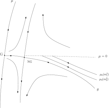
Figure 3: Schematic depiction of the flow until the mass scale, for two masses $m_{1}^{2}>m_{2}^{2}>0$. For $m^{2}=0$, the flow lies on the stable manifold and flows to the non-Gaussian RG fixed point NG.

7.2 Flow until mass scale

Throughout this section, our focus is on scales $j\leq j_{m}$. We permit $m^{2}=0$, in which case $j\leq j_{m}$ means $j<j_{0}=\infty$. We take $L$ large, then choose $\epsilon$ (hence $\bar{s}$) small depending on $L$, and often do this in the following without explicit mention.

The construction of the global flow is via the identification of a fixed point for a map $T$ on a certain Banach space, which we introduce in this section. We define the space $X$ and map $T$ using the infinite-volume version ($\mathbb{V}={{{\mathbb{Z}}}^{d}}$) of the maps $K_{+},R_{+}$. In this way we avoid dependence on the volume parameter $N$, for the map $T$ and its fixed point. On the other hand, the fixed point for the infinite-volume flow immediately produces a flow for the finite torus $\mathbb{V}=\Lambda_{N}$ over all scales $0\leq j\leq N$. This is because the infinite-volume RG map obeys the same estimates as the finite-volume RG map in Theorem 6.4, so the finite-volume RG map can be iterated over as many scales as the infinite-volume RG map, from the same initial condition.

7.2.1 The Banach space $X$

Let $\mathcal{W}_{j}^{*}$ denote the Banach space with norm (6.28) defined for the infinite volume $\mathbb{V}={{{\mathbb{Z}}}^{d}}$ and for $m^{2}=0$. Let $E_{j}={\mathbb{R}}$ and let $F_{j}={\mathbb{R}}\times\mathcal{W}_{j}^{*}$, so $\mu_{j}\in E_{j}$ and $(y_{j},K_{j})\in F_{j}$. Let $X_{0}=E_{0}$, $X_{j}=E_{j}\times F_{j}$ for $j>0$. The Banach space of interest is $X=\oplus_{j=0}^{\infty}X_{j}$. An initial condition specifies $(y_{0},K_{0})\in F_{0}$, and $F_{0}$ is not part of the space $X$. We only need the case $K_{0}=\mathbbm{1}_{\varnothing}$, which we assume in the following. The initial condition $y_{0}$ is determined by the parameter $g$ appearing in the statements of Theorems 1.1–1.2, via $y_{0}=\bar{s}-g_{0}=\bar{s}-g$, with $\bar{s}$ the perturbative fixed point given in (5.49).

The norm on $X$ is defined in terms of weights ${\sf w}$, by

$$\|(\mu,y,K)\|=\max\left\{\sup_{j\geq 0}{\sf w}_{\mu}^{-1}|\mu_{j}|,\;\sup_{j\geq 1}{\sf w}_{y,j}^{-1}|y_{j}|,\;\sup_{j\geq 1}{\sf w}_{K}^{-1}\|K_{j}\|_{\mathcal{W}_{j}^{*}}\right\}.$$ (7.17)

The weights are

$${\sf w}_{\mu}=\sigma\bar{s}^{2},\quad{\sf w}_{y,j}=\omega_{j}\bar{s},\quad{\sf w}_{K}=\lambda\bar{s}^{3},$$ (7.18)

where $\sigma,\omega_{j},\lambda>0$ are chosen as follows. With $\pi_{j}=\pi_{j}(m^{2})$ given by (5.14), we define $\sigma$ by

$$\sigma=5\Pi,\quad\quad\Pi=\sup_{m^{2}\in[0,1]}\sup_{j\geq 0}|\pi_{j}|<\infty.$$ (7.19)

With the constant $C_{\rm RG}$ of Theorem 6.4, we set

$$\lambda=C_{\rm RG}.$$ (7.20)

To define the weight $\omega_{j}$, let $J_{L}$ and $b_{L}$ be given by Lemma 5.5. Let $\zeta=1-64b_{L}\bar{s}<1$, $\omega=\frac{1}{32}$, and

$$\omega_{j}=\omega\zeta^{(J_{L}-j)_{+}}.$$ (7.21)

By definition, $\omega_{j}=\omega$ when $j\geq J_{L}$, and, for all $j$,

$$\omega_{0}=\omega\zeta^{J_{L}}\leq\omega_{j}\leq\omega.$$ (7.22)

Since $\epsilon$ can be chosen small depending on $L$, we have $\zeta^{J_{L}}=1-O(\epsilon)$, so $\omega_{j}$ remains within order $\epsilon$ of $\omega$ for all $j$. It is via this choice of weight that we deal with transient lattice effects near scale $0$; this avoids an analysis as in [79, Theorem 6.3].

We write $B_{1}=B_{1}(X)$ for the closed unit ball in $X$. The assumption that $x=(\mu,y,K)\in B_{1}$ implies in particular that $|\mu_{j}|\leq\sigma\bar{s}^{2}$, that $|s_{j}|=|\bar{s}-y_{j}|\leq(1+\omega)\bar{s}=\frac{33}{32}\bar{s}$, and that $\|K_{j}\|\leq C_{\rm RG}\bar{s}^{3}\leq 4C_{\rm RG}\bar{s}^{3}$. Therefore,

$$x=(\mu,y,K)\in B_{1}\quad\Rightarrow\quad(g_{j},\nu_{j},K_{j})\in\mathbb{D}_{j}\;\;\text{for all $j$}.$$ (7.23)

By definition, the space $X$, including its norm, does not depend $m^{2}$. Moreover, for $m^{2}>0$, the space $\mathcal{W}_{j}$ defined with mass $m^{2}$ is identical to the space $\mathcal{W}_{j}$ defined with mass zero as long as $j\leq j_{m}$. This follows from the fact that the massive and massless versions of the parameters $\ell_{j},h_{j},\bar{\epsilon}_{j},\gamma_{j}$ are identical below the mass scale defined for $m^{2}>0$ (the parameters are defined in (3.20), (6.24), (6.25), (6.27)). Thus, although we have defined $X$ in terms of $\mathcal{W}_{j}^{*}$ with zero mass, it would be equivalent when $m^{2}>0$ to use $\mathcal{W}_{j}$ defined with $m^{2}$ instead, as long as $j\leq j_{m}$.

7.2.2 The map $T$

Next, we define a map $T:X\rightarrow X$.

We are interested in $m^{2}\in[0,\delta]$ with $\delta$ small, so we may assume that $j_{m}\geq j_{\delta}>2J_{L}$. In addition to the transient lattice effects handled via the weights (7.21), there are also transient effects near scale $j_{m}$ when $m^{2}>0$ (effect of nonzero mass). We define $T$ in such a manner that avoids dealing with the latter effects, whose treatment is postponed.

Let

$$M_{\mathrm{ext}}=\{(\tilde{m}^{2},m^{2})\in(0,\infty)\times[0,\delta]:j_{\tilde{m}}\leq j_{m}-(J_{L}+2)\}.$$ (7.24)

We regard $M_{\mathrm{ext}}$ as a metric space, with metric induced from ${\mathbb{R}}^{2}$. Note that $\tilde{m}^{2}=0$ is excluded from $M_{\mathrm{ext}}$. For $m^{2}>0$, the point $(\tilde{m}^{2},m^{2})$ lies in $M_{\mathrm{ext}}$ if and only if $\tilde{m}^{2}\in[m^{2}_{-},\infty)$, where $m^{2}_{-}$ (a function of $m^{2}$) is the least value of $u^{2}$ for which $j_{u}=j_{m}-(J_{L}+2)$.

Fix $(\tilde{m}^{2},m^{2})\in M_{\mathrm{ext}}$ or $(\tilde{m}^{2},m^{2})=(0,0)$. Given $(y_{0},K_{0})\in F_{0}$ with $|y_{0}|\leq\omega_{0}\bar{s}$ and $K_{0}=\mathbbm{1}_{\varnothing}$, we define a map $\hat{T}:B_{1}\rightarrow X$, with $\hat{T}=(\hat{T}^{(\mu)},\hat{T}^{(y)},\hat{T}^{(K)})$, by setting $(\hat{T}x)_{j}=0$ if $j>j_{\tilde{m}}$, whereas for $1\leq j\leq j_{\tilde{m}}$ we define

$$(\hat{T}^{(\mu)}x)_{j} =L^{-\alpha}(\mu_{j+1}-\rho_{\mu,j}-r_{\mu,j}),$$ (7.25)

$$(\hat{T}^{(y)}x)_{j} =c_{\epsilon}y_{j-1}+aL^{\epsilon}y_{j-1}^{2}+(\beta^{:}_{j-1}-a)L^{\epsilon}(\bar{s}-y_{j-1})^{2}+r_{y,j-1},$$ (7.26)

$$(\hat{T}^{(K)}x)_{j} =\check{K}_{j}(\mu_{j-1},y_{j-1},K_{j-1}).$$ (7.27)

On the right-hand side, $\rho_{\mu,j},\beta^{:}_{j-1},r_{\mu,j},r_{y,j-1},\check{K}_{j}$ are defined with mass $m^{2}$ ($r_{\mu,j},r_{y,j-1}$ are determined by the map $R_{+}$). By (7.23), the hypotheses of Theorem 6.4 are satisfied and $r_{\mu},r_{y},\check{K}$ are well-defined on the right-hand side of (7.25)–(7.27).

Observe that a fixed point of $\hat{T}$, i.e., a solution to $\hat{T}x=x$, defines a flow satisfying (7.10)–(7.12) up to scale $j_{\tilde{m}}$, with initial condition given by $(y_{0},\mathbbm{1}_{\varnothing})$, and with final condition $\mu_{j_{\tilde{m}}+1}=0$ when $\tilde{m}^{2}>0$. When $\tilde{m}^{2}=m^{2}=0$, no final condition is imposed.

We desire continuity on $M_{\mathrm{ext}}$, but $\hat{T}$ jumps as $\tilde{m}$ varies through values where $j_{\tilde{m}}$ jumps. Recall from (3.16) that $j_{\tilde{m}}=\lceil f_{\tilde{m}}\rceil$, and let

$$\delta_{\tilde{m}}=j_{\tilde{m}}-f_{\tilde{m}}=\lceil f_{\tilde{m}}\rceil-f_{\tilde{m}}\in[0,1),$$ (7.28)

which is a sawtooth function of $\tilde{m}$. We smooth out the jump in $\hat{T}$ at scale $j_{\tilde{m}}$ to get continuity in $\tilde{m}$. This is done by setting $T_{j}=\hat{T}_{j}$ for all $j\neq j_{\tilde{m}}+1$, and instead of $\hat{T}_{j_{\tilde{m}}+1}=0$, we define

$$(T^{(\mu)}x)_{j_{\tilde{m}}+1} =(1-\delta_{\tilde{m}})L^{-\alpha}(\mu_{j_{\tilde{m}}+2}-\rho_{\mu,j_{\tilde{m}}+1}-r_{\mu,j_{\tilde{m}}+1}),$$ (7.29)

$$(T^{(y)}x)_{j_{\tilde{m}}+1} =(1-\delta_{\tilde{m}})\left(c_{\epsilon}y_{j_{\tilde{m}}}+aL^{\epsilon}y_{j_{\tilde{m}}}^{2}+(\beta^{:}_{j_{\tilde{m}}}-a)L^{\epsilon}(\bar{s}-y_{j_{\tilde{m}}})^{2}+r_{y,j_{\tilde{m}}}\right),$$ (7.30)

$$(T^{(K)}x)_{j_{\tilde{m}}+1} =(1-\delta_{\tilde{m}})\check{K}_{j_{\tilde{m}}+1}(\mu_{j_{\tilde{m}}},y_{j_{\tilde{m}}},K_{j_{\tilde{m}}}).$$ (7.31)

For $(\tilde{m}^{2},m^{2})=(0,0)$, we have $j_{0}=\infty$ and $T_{j}=\hat{T}_{j}$ for all $j$, but we do not consider continuity of $T$ at $(\tilde{m}^{2},m^{2})=(0,0)$. The following lemma provides the continuity statement that we need for the map $T$.

Lemma 7.2.

For each $x\in B_{1}(X)$, $Tx$ is a continuous function of $(\tilde{m}^{2},m^{2})\in M_{\mathrm{ext}}$ into $X$.

Proof.

It suffices to prove the continuity of $(Tx)_{j}$ for each $j$. The continuity of $(Tx)_{j}$ in $m^{2}\in[0,\delta]$ is not the difficulty. It follows from the continuity of $\beta^{:},\beta,\pi$ (the latter two are in $\rho_{\mu}$) due to Lemma 5.2, together with the continuity in $m^{2}$ provided by Theorem 6.4 for the remainders $r_{*}$ and the map $K_{+}$. (The continuity provided by Theorem 6.4 is for $m^{2}\leq[0,L^{-\alpha j}]$, so $j\leq j_{m}$, and this is satisfied here since the nonzero $T_{j}$ have $j\leq j_{\tilde{m}}+1<j_{m}$.)

Discontinuities in $\tilde{m}^{2}$ can only occur at values $\tilde{m}_{*}$ where $j_{\tilde{m}}$ makes its jumps, namely values where $\delta_{\tilde{m}_{*}}=0$. By definition, $\delta_{\tilde{m}}\downarrow 0$ as $\tilde{m}\downarrow\tilde{m}_{*}$, whereas $\delta_{\tilde{m}}\uparrow 1$ as $\tilde{m}\uparrow\tilde{m}_{*}$, and $j_{\tilde{m}}$ increases its value from $j_{\tilde{m}_{*}}$ to $j_{\tilde{m}_{*}}+1$ as $\tilde{m}$ decreases through $\tilde{m}_{*}$. The effect of the factors $(1-\delta_{j_{\tilde{m}}})$ in (7.29)–(7.31) is to continuously acquire the terms that occur discontinuously in $\hat{T}$ when $\tilde{m}$ varies through values where $j_{\tilde{m}}$ jumps. To see this, consider a small neighbourhood $N\ni\tilde{m}_{*}$, containing no other point of discontinuity. Let $\tilde{m}\in N$. If $\tilde{m}>\tilde{m}_{*}$, then $j_{\tilde{m}}=j_{\tilde{m}_{*}}$, and taking the limit as $\tilde{m}\downarrow\tilde{m}_{*}$ in (7.29)–(7.31) gives

$$(T^{(\mu)}x)_{j_{\tilde{m}_{*}}+1} =L^{-\alpha}(\mu_{j_{\tilde{m}_{*}}+2}-\rho_{\mu,j_{\tilde{m}_{*}+1}}-r_{\mu,j_{\tilde{m}_{*}}+1}),$$ (7.32)

$$(T^{(y)}x)_{j_{\tilde{m}_{*}}+1} =c_{\epsilon}y_{j_{\tilde{m}_{*}}}+aL^{\epsilon}y_{j_{\tilde{m}_{*}}}^{2}+(\beta^{:}_{j_{\tilde{m}_{*}}}-a)L^{\epsilon}(\bar{s}-y_{j_{\tilde{m}_{*}}})^{2}+r_{y,j_{\tilde{m}_{*}}},$$ (7.33)

$$(T^{(K)}x)_{j_{\tilde{m}_{*}}+1} =\check{K}_{j_{\tilde{m}_{*}}+1}(\mu_{j_{\tilde{m}_{*}}},y_{j_{\tilde{m}_{*}}},K_{j_{\tilde{m}_{*}}}).$$ (7.34)

For $\tilde{m}<\tilde{m}_{*}$, we have $j_{\tilde{m}_{*}}+1=j_{\tilde{m}}$, so $(Tx)_{j_{\tilde{m}}}$ is given by (7.25)–(7.27), and its limit as $\tilde{m}\uparrow\tilde{m}_{*}$ agrees with the limit $\tilde{m}\downarrow\tilde{m}_{*}$. In addition, if $\tilde{m}<\tilde{m}_{*}$ then $j_{\tilde{m}}=j_{\tilde{m}_{*}}+1$, and taking the limit as $\tilde{m}\uparrow\tilde{m}_{*}$ in (7.29)–(7.31) gives

$$(T^{(\mu)}x)_{j_{\tilde{m}_{*}}+2} =0,$$ (7.35)

$$(T^{(y)}x)_{j_{\tilde{m}_{*}}+2} =0,$$ (7.36)

$$(T^{(K)}x)_{j_{\tilde{m}_{*}}+2} =0.$$ (7.37)

This shows the required continuity of $(Tx)_{j}$ as $\tilde{m}$ varies through $j_{\tilde{m}_{*}}$.  

7.2.3 Contractivity of $T$

The dynamical system defined by $T$ is hyperbolic, in contrast to the more difficult non-hyperbolic system for $d=4$ analysed in [17]. Our analysis of $T$ is inspired by [32, 79], as well as by the stable manifold theorem of [27, Theorem 2.16]. It bears resemblance to the analysis used for the massless case in [24, 32, 79], e.g., [32, Section 6], but there are differences. In particular, we consider the massive case. Also, [24, 32] work in the continuum where lattice effects are absent. We do not need to deal separately with lattice effects at small scales, as was done via an additional application of the implicit function theorem in [79, Theorem 6.3]. Instead, lattice transients are handled via our choice of weights $\omega_{j}$.

The following theorem proves that $T$ is a contraction. As usual, we fix $L$ large enough and then choose $\epsilon$ small enough depending on $L$. Continuity of $T$ in $M_{\mathrm{ext}}$ is not needed for Theorem 7.3, but is used in Corollary 7.5.

Theorem 7.3.

Let $(\tilde{m}^{2},m^{2})\in M_{\mathrm{ext}}$, or $\tilde{m}^{2}=m^{2}=0$. For every initial condition $(y_{0},\mathbbm{1}_{\varnothing})\in F_{0}$ with $|y_{0}|\leq\omega_{0}\bar{s}$, we have $T:B_{1}\rightarrow B_{1}$, and there exists $c\in(0,1)$ (depending on $\epsilon,L$, independent of $(\tilde{m}^{2},m^{2})$) such that $\|DT\|\leq c$ on $B_{1}$.

Proof.

Recall the definitions of the weights in (7.18)–(7.21). Suppose $x\in B_{1}$. Then, for all $j$,

$$|\mu_{j}|\leq\sigma\bar{s}^{2},\quad|y_{j}|\leq\omega_{j}\bar{s}\leq\omega\bar{s},\quad\|K_{j}\|\leq\lambda\bar{s}^{3}.$$ (7.38)

By (7.23), $(g_{j},\nu_{j},K_{j})\in\mathbb{D}_{j}$ for all $j$.

Bound on $T$. We verify that $T:B_{1}\rightarrow B_{1}$. First, we have (by Theorem 6.4 for $T^{(K)}$)

$$|(T^{(\mu)}x)_{j}| \leq L^{-\alpha}\sigma\bar{s}^{2}+\Pi\bar{s}^{2}+O(\bar{s}^{3})\leq\sigma\bar{s}^{2},$$ (7.39)

$$|(T^{(K)}x)_{j}| \leq C_{\rm RG}\bar{s}^{3}=\lambda\bar{s}^{3}.$$ (7.40)

For the more delicate component, we start with

$$|(T^{(y)}x)_{j}| \leq\omega_{j}\bar{s}\frac{\omega_{j-1}}{\omega_{j}}\Big{(}c_{\epsilon}+aL^{\epsilon}\omega_{j-1}\bar{s}+\omega_{j-1}^{-1}|\beta_{j}^{:}-a|L^{\epsilon}(1+\omega_{j-1})^{2}\bar{s}+O(\bar{s}^{2})\Big{)}.$$ (7.41)

Recall from (5.50) that $a\bar{s}\sim\epsilon\log L$, and that $\zeta$ in (7.21) is given by $\zeta=1-64b_{L}\bar{s}$. By Lemma 5.5, for scales $j\leq J_{L}$ we have $|\beta_{j}^{:}-a|\leq b_{L}$, whereas for $j_{L}\leq j\leq j_{m}-J_{L}$ we have $|\beta_{j}^{:}-a|\leq\frac{a}{64}$. In the former case, (7.41) gives

$$|(T^{(y)}x)_{j}| \leq\omega_{j}\bar{s}\zeta\Big{(}1-\epsilon\log L(1-\tfrac{1}{31})+33b_{L}(\tfrac{17}{16})^{2})\bar{s}\Big{)}$$

$$\leq\omega_{j}\bar{s}\zeta(1+\tfrac{3}{4}64b_{L}\bar{s})\leq\omega_{j}\bar{s}.$$ (7.42)

For larger scales, we have instead that

$$|(T^{(y)}x)_{j}| \leq\omega_{j}\bar{s}\Big{(}1-\epsilon\log L(1-\tfrac{1}{31}-33\tfrac{1}{64}(\tfrac{17}{16})^{2})\Big{)}\leq\omega_{j}\bar{s}.$$ (7.43)

Thus, in either case,

$$|(T^{(y)}x)_{j}| \leq\omega_{j}\bar{s},$$ (7.44)

and with (7.39)–(7.40) and (7.44) we conclude that $T:B_{1}\rightarrow B_{1}$.

Bound on $DT$. To prove that there exists $c<1$ such that $\|DT(x)\|\leq c$ for $x\in B_{1}$, it suffices to prove that $\|D_{\mu}T^{(*)}(x)\|+\|D_{y}T^{(*)}(x)\|+\|D_{K}T^{(*)}(x)\|\leq c$ for $*=\mu,y,K$. This is a consequence of the following estimates. The crucial step is (7.50), which is provided by Theorem 6.4. The delicate step which requires attention here is (7.2.3), and its proof is similar to that of (7.44). Differentiation of $T$ gives (recall $\lambda=C_{\rm RG}$ and (7.13))

$$\|D_{\mu}T^{(\mu)}(x)\| =\sup_{j}\frac{\sigma\bar{s}^{2}}{\sigma\bar{s}^{2}}|D_{\mu}(T^{(\mu)}(x))_{j}|\leq L^{-\alpha}+O(\bar{s})\leq\tfrac{1}{2},$$ (7.45)

$$\|D_{y}T^{(\mu)}(x)\| =\sup_{j}\frac{\omega_{j-1}\bar{s}}{\sigma\bar{s}^{2}}|D_{y}(T^{(\mu)}(x))_{j}|$$

$$\leq\frac{\omega\bar{s}}{\sigma\bar{s}^{2}}(4\Pi\bar{s}+O(\bar{s}^{2}))=\omega\left(\tfrac{4}{5}+O(\bar{s})\right)\leq\tfrac{1}{32},$$ (7.46)

$$\|D_{K}T^{(\mu)}(x)\| \leq\frac{\lambda\bar{s}^{3}}{\sigma\bar{s}^{2}}O(1)\leq O(\bar{s})\leq\tfrac{1}{4},$$ (7.47)

$$\|D_{\mu}T^{(K)}(x)\| \leq\frac{\sigma\bar{s}^{2}}{\lambda\bar{s}^{3}}O(\bar{s}^{2})\leq O(\bar{s})\leq\tfrac{1}{4},$$ (7.48)

$$\|D_{y}T^{(K)}(x)\| \leq\sup_{j}\frac{\omega_{j-1}\bar{s}}{\lambda\bar{s}^{3}}C_{\rm RG}\bar{s}^{2}=\omega=\tfrac{1}{32},$$ (7.49)

$$\|D_{K}T^{(K)}(x)\| \leq\frac{\lambda\bar{s}^{3}}{\lambda\bar{s}^{3}}\kappa=\kappa\leq\tfrac{1}{4},$$ (7.50)

$$\|D_{\mu}T^{(y)}(x)\| \leq\sup_{j}\frac{\sigma\bar{s}^{2}}{\omega_{j}\bar{s}}O(\bar{s}^{2})\leq O(\bar{s}^{3}),$$ (7.51)

$$\|D_{K}T^{(y)}(x)\| \leq\sup_{j}\frac{\lambda\bar{s}^{3}}{\omega_{j}\bar{s}}O(1)\leq O(\bar{s}^{2}).$$ (7.52)

Finally, again using $a\bar{s}\sim\epsilon\log L$, we have

$$\|D_{y}T^{(y)}(x)\| =\sup_{j}\frac{\omega_{j-1}\bar{s}}{\omega_{j}\bar{s}}|D_{y}(T^{(y)}(x))_{j}|$$

$$\leq\sup_{j}\frac{\omega_{j-1}}{\omega_{j}}\left(c_{\epsilon}+2aL^{\epsilon}\omega_{j-1}\bar{s}+|\beta^{:}_{j-1}-a|L^{\epsilon}2(1+\omega_{j-1})\bar{s}+O(\bar{s}^{2})\right)$$

$$\leq\sup_{j}\frac{\omega_{j-1}}{\omega_{j}}\left(1+\epsilon\log L(-1+\tfrac{1}{8})+|\beta^{:}_{j-1}-a|2\tfrac{17}{16}\bar{s}\right).$$ (7.53)

Suppose first that $j\leq J_{L}$, so that $|\beta^{:}_{j-1}-a|\leq b_{L}$ by (5.21). With $\zeta=1-64b_{L}\bar{s}$, we see that the argument of the supremum is bounded above by

$$\zeta\left(1+\tfrac{17}{8}b_{L}\bar{s}\right)\leq 1-32b_{L}\bar{s}.$$ (7.54)

On the other hand, if $J_{L}<j<j_{m}-J_{L}$, then we have $|\beta^{:}_{j-1}-a|\leq\frac{a}{64}$ by Lemma 5.3, and hence (since $\omega_{j-1}=\omega_{j}$ by definition) the bound becomes

$$1+\epsilon\log L\Big{(}-1+\tfrac{1}{8}+\tfrac{1}{16}\Big{)}\leq 1-\tfrac{3}{4}\epsilon\log L.$$ (7.55)

Each of (7.54)–(7.55) remains less than $1$ after addition of the bounds in (7.51)–(7.52), and the proof is complete.  

Remark 7.4.

Restriction on $g$. By definition, $\omega_{0}=\omega(1-O(\epsilon))$. In particular, $\omega_{0}\geq\textstyle{\frac{1}{2}}\omega=\frac{1}{64}$. The restriction $|y_{0}|\leq\omega_{0}\bar{s}$ in Theorem 7.3 is therefore satisfied if $g=g_{0}=\bar{s}-y_{0}$ obeys

$$|g-\bar{s}|\leq\tfrac{1}{64}\bar{s}.$$ (7.56)

This restriction on $g$ is incorporated into the statements of Theorems 1.1–1.2. It is clear that the constant $\frac{1}{64}$ could be improved.

7.2.4 Flow until mass scale and construction of critical initial value

Let $|y_{0}|\leq\omega_{0}\bar{s}$, and let $(\tilde{m}^{2},m^{2})\in M_{\mathrm{ext}}$ with $M_{\mathrm{ext}}$ defined in (7.24), or let $(\tilde{m}^{2},m^{2})=(0,0)$. Together with the contraction mapping principle, Theorem 7.3 implies that $T$ has a unique fixed point $x^{c}\in B_{1}$, i.e., $Tx^{c}=x^{c}$. This fixed point provides a solution to the flow equations (7.10)–(7.12) that maintains $(g_{j},\nu_{j},K_{j})$ in the RG domain $\mathbb{D}_{j}$ for all scales $0\leq j\leq j_{\tilde{m}}$. For the case $\tilde{m}^{2}=m^{2}=0$, this is a flow on all scales. In either case, we write the $\mu$-component of the initial value $x_{0}^{c}$ as

$$\mu_{0}(\tilde{m}^{2},m^{2})=(x_{0}^{c})^{(\mu)}(\tilde{m}^{2},m^{2}).$$ (7.57)

For $m^{2}>0$, the minimal value for $\tilde{m}^{2}$ in $M_{\mathrm{ext}}$ is such that $j_{\tilde{m}}=j_{m}-(J_{L}+2)$, so in this case the flow does not quite reach $j_{m}$, but fails to do so by only a bounded ($L$-dependent) number of scales. As in the discussion below (7.24), we write this minimal value of $\tilde{m}^{2}$ as $m^{2}_{-}=m^{2}_{-}(m^{2})$. Then we define the critical initial value

$$\mu_{0}(m^{2})=\mu_{0}(m_{-}^{2},m^{2})\quad(m^{2}>0),$$ (7.58)

i.e., $\mu_{0}(m^{2})$ is the $\mu$-component of $x_{0}^{c}$ for $T$ defined with $(\tilde{m}^{2},m^{2})=(m^{2}_{-},m^{2})\in M_{\mathrm{ext}}$. For $\tilde{m}^{2}=m^{2}=0$, which is also permitted in Theorem 7.3, we denote the critical initial value by $\mu_{0}(0)=\mu_{0}(0,0)$. The following corollary to Theorem 7.3 gives continuity of $\mu_{0}(m^{2})$ in $m^{2}\in(0,\delta]$.

Corollary 7.5.

The function $\mu_{0}(\tilde{m}^{2},m^{2})$ is continuous in $(\tilde{m}^{2},m^{2})\in M_{\mathrm{ext}}$. In particular, $\mu_{0}(m^{2})$ is continuous in $m^{2}\in(0,\delta]$.

Proof.

By Lemma 7.2, $Tx$ is jointly continuous in $(\tilde{m}^{2},m^{2})\in M_{\mathrm{ext}}$, for each $x\in B_{1}$, and $T$ is uniformly contractive. By the version of the contraction mapping principle given in [72, Corollary 4, p.230], the fixed point of $T$ is continuous in $(\tilde{m}^{2},m^{2})\in M_{\mathrm{ext}}$. In particular, so is $\mu_{0}(\tilde{m}^{2},m^{2})$, and therefore $\mu_{0}(m^{2})$ is continuous in $m^{2}\in(0,\delta]$.  

The next corollary makes the important extension of Corollary 7.5 to include right-continuity at $m^{2}=0$.

Corollary 7.6.

The limit $\lim_{m^{2}\downarrow 0}\mu_{0}(m^{2})$ exists and equals $\mu_{0}(0)$ (the critical initial value for the case $\tilde{m}^{2}=m^{2}=0$).

Proof.

Fix $y_{0}$ with $|y_{0}|\leq\omega_{0}\bar{s}$, fix a sequence $m^{\prime}\downarrow 0$, and let $x_{0}^{\prime}=(\mu_{0}(m^{\prime}),y_{0},\mathbbm{1}_{\varnothing})\in E\times F_{0}$. Since $\mu_{0}(m^{\prime})$ remains in a bounded subset of ${\mathbb{R}}$, it has a limit point $\mu_{0}^{*}$. It suffices to show that $\mu_{0}^{*}=\mu_{0}(0)$, for any sequence $m^{\prime}$.

Let $x_{0}^{*}=(\mu_{0}^{*},y_{0},\mathbbm{1}_{\varnothing})$. We use $x_{0}^{*}$ as the initial condition for the flow equations (7.10)–(7.12), and we solve those flow equations inductively, to produce $x_{j}^{*}$, for as long as this remains in the closed unit ball $B_{1}(X_{j})$ (with norm on $X_{j}$ given by (7.17) with the suprema over $j$ omitted). On the other hand, with initial condition $x_{0}^{\prime}$ the fixed point solves the equations for $j\leq j_{m^{\prime}_{-}}$, with $x_{j}^{\prime}\in B_{1}(X_{j})$. Given any fixed $j$, eventually $j<j_{m^{\prime}_{-}}$ as $m^{\prime}\downarrow 0$. By the continuity of the RG map (6.32) at $m^{2}=0$ (recall Theorem 6.4), we know that $x_{j}^{\prime}$ converges to $x_{j}^{*}$, which must remain in the closed ball $B_{1}(X_{j})$. This produces a sequence $x_{j}^{*}$ for all $j<\infty$, which is a solution of the zero-mass flow equations for all $j$, and hence a fixed point of the zero-mass $T$. This fixed point is unique, and $x_{0}^{*}=(\mu_{0}(0),y_{0},\mathbbm{1}_{\varnothing})$. Therefore, $\mu_{0}^{*}=\mu_{0}(0)$, and the proof is complete.  

Remark 7.7.

The RG fixed point NG in Figure 3 will correspond to the limits

$$s_{\infty} =s_{\infty}(0)=\lim_{j\rightarrow\infty}s_{j}(0),\quad\mu_{\infty}=\mu_{\infty}(0)=\lim_{j\rightarrow\infty}\mu_{j}(0)$$ (7.59)

for the massless flow. We do not prove existence of these limits, and we do not need or use it, but it would be of interest to explore this further.

The space $X$ is defined in terms of the massless infinite-volume RG map, and in particular involves the norm $\mathcal{W}^{*}$. However, since we only consider scales below the mass scale, for $m^{2}>0$ the bounds for all massless norms are identical to those for the massive case. Also, since Theorem 6.4 provides the same estimates for either the finite- or infinite-volume RG maps, the infinite-volume flow also gives rise to a finite-volume flow by iterating the finite-volume RG map from the initial condition given by the fixed point of $T$. Thus there is no distinction between existence of finite- or infinite-volume flows up to the mass scale.

For $m^{2}>0$, the fixed point of the map $T$ produces a flow $x_{j}\in B_{1}(X_{j})$ for scales $j\leq j_{m_{-}}=j_{m}-J_{L}$. We wish to extend this to a flow for all scales $j<\infty$. The following lemma does a small portion of this, by extending to scales $j\leq j_{m}$. The full extension is provided by Theorem 7.9.

Lemma 7.8.

Let $m^{2}\in(0,\delta]$, and let $(x_{j})_{j\leq j_{m}-J_{L}}$ be the RG flow produced by Theorem 7.3. This flow extends to a flow $(\mu_{j},y_{j},K_{j})_{j\leq j_{m}}$ for all $j\leq j_{m}$, with $|\mu_{j}|\leq c_{L}\bar{s}^{2}$, $|y_{j}|\leq\frac{1}{31}\bar{s}$, and $\|K_{j}\|_{\mathcal{W}_{j}}\leq C_{\rm RG}\bar{s}^{3}$, where $c_{L}$ is an $L$-dependent constant.

Proof.

We solve the flow equations (7.10)–(7.12) forward until scale $j_{m}$, starting from scale $j_{m}-J_{L}$. This can be done as long as $(g_{j},\nu_{j},K_{j})\in\mathbb{D}_{j}$. The number of scales to be advanced is $J_{L}$, which is independent of $m^{2}$ and $\epsilon$. At each step, the bound on $\mu_{j}$ deteriorates by an $L$-dependent factor. In fact, by (7.10) and (7.19), if $|\mu_{j}|\leq t\bar{s}^{2}$ then (we may assume $t\geq 1$)

$$|\mu_{j+1}|\leq L^{\alpha}(t\bar{s}^{2}+\Pi 4\bar{s}^{2})\leq L^{\alpha}(1+4\Pi)t\bar{s}^{2}.$$ (7.60)

For $y_{j}$, by Lemma 5.5 we have $|\beta_{j}^{:}-a|\leq b_{L}$. From (7.11), we obtain

$$|y_{j+1}|\leq|y_{j}|(1+aL^{\epsilon}|y_{j}|)+4b_{L}\bar{s}^{2}.$$ (7.61)

Thus a bound $|y_{j}|\leq t\bar{s}$ yields a bound $|y_{j+1}|\leq(1+c_{L}^{\prime}\bar{s})t\bar{s}$, so the deterioration is $1+c_{L}^{\prime}\bar{s}$ per scale. The accumulation of these deteriorations, which multiply over scales, is some constant $c_{L}=(L^{\alpha}(1+4\Pi))^{J_{L}}$ for $\mu$ and $(1+c_{L}^{\prime}\bar{s})^{J_{L}}\leq 1+c_{L}^{\prime\prime}\bar{s}$ for $y$. These accumulated effects cannot move $(g_{j},\nu_{j})$ out of $\mathcal{D}_{j}$, since $|y_{j}|$ remains less than $(1+O(\bar{s}))\frac{1}{32}\bar{s}$, and $\mu_{j}$ is an $O(\bar{s}^{2})$ adjustment to the leading term $-\eta_{\geq j}\bar{s}$ in $\hat{\mu}_{j}$ (recall (5.34)). Theorem 6.4 then guarantees that (7.10)–(7.12) can indeed by iterated forward until scale $j_{m}$, as required.  

7.3 Flow beyond mass scale

Theorem 7.3 and Lemma 7.8 produce a flow that exists up to the mass scale. Beyond the mass scale, there is exponential decay in the flow equations which makes it possible to obtain a solution by forward iteration without further tuning. This is accomplished in the next theorem. Its hypothesis that $m^{2}\geq L^{-\alpha(N-1)}$ ensures that $C_{N,N}$ obeys a bound $L^{-(N-1)(d-\alpha)}$, by (3.12). To study the flow past $j_{m}$, we extend the definition of $\hat{\mu}_{j}$, given in (5.26) for $j\leq j_{m}$, and define a corresponding remainder term $r_{\hat{\mu},j}$, by

$$\hat{\mu}_{j}=L^{\alpha j_{m}}\nu_{j},\quad r_{\hat{\mu},j}=L^{\alpha j_{m}}r_{\nu,j},\quad(j\geq j_{m}).$$ (7.62)

By definition, $\hat{g}_{j_{m}}=L^{\epsilon j_{m}}g_{j_{m}}$. After some algebra, the flow equation for $\nu_{j}$ given in (7.2) can be equivalently written, for $j\geq j_{m}$, as

$$\hat{\mu}_{j+1}-\hat{\mu}_{j} =L^{-(d-\alpha)(j-j_{m})}\eta_{j}\hat{g}_{j_{m}}(1+4\hat{\mu}_{j}\bar{w}_{j}^{(1)})-L^{-(\alpha-2\epsilon)(j-j_{m})}\xi_{j}\hat{g}_{j_{m}}^{2}-\bar{\gamma}\beta_{j}\hat{g}_{j_{m}}\hat{\mu}_{j}$$

$$\quad-\Big{[}\hat{\mu}_{j}^{2}L^{-\alpha j_{m}}C_{j+1}^{(1)}+2L^{-(d-\alpha)(j-j_{m})}\eta_{j}\hat{\mu}_{j}\hat{g}_{j_{m}}\bar{w}_{j+1}^{(1)}$$ (7.63)

$$\quad\quad\quad+(L^{-(d-\alpha)(j-j_{m})}\eta_{j}\hat{g}_{j_{m}})^{2}\bar{w}_{j+1}^{(1)}\Big{]}+r_{\hat{\mu},j}.$$

Theorem 7.9.

Let $m^{2}\in[L^{-\alpha(N-1)},\delta]$ and $g\in[\frac{63}{64}\bar{s},\frac{65}{64}\bar{s}]$. With initial condition at $j=j_{m}$ produced by Lemma 7.8, the flow equations for $(g_{j},\nu_{j},K_{j})$ can be solved forward (inductively) to scale $N$, and produce a sequence which remains in the domain $\mathbb{D}_{j}$ for each $j$. For $g_{j}$, we have simply $g_{j}=g_{j_{m}}$ for all $j\geq j_{m}$ and the limit $g_{\infty}=\lim_{N\rightarrow\infty}g_{N}=g_{j_{m}}\in[\frac{15}{16}L^{-\epsilon j_{m}}\bar{s},\frac{17}{16}L^{-\epsilon j_{m}}\bar{s}]$ exists. For $\nu_{j}$, the limit $\nu_{\infty}=\lim_{N\rightarrow\infty}\nu_{N}=O(L^{-\alpha j_{m}}\bar{s})$ exists, and is attained uniformly on compact subsets of $m^{2}\in(0,\delta]$. Moreover, $(\nu_{j})_{j\leq N}$ is independent of the volume in the sense that it is identical up to scale $N$ with the sequence $(\nu_{j})_{j\leq N^{\prime}}$ for any $N^{\prime}>N$.

Proof.

We first consider the initial conditions. By Lemma 7.8, $|y_{j_{m}}|\leq\omega\bar{s}=\frac{1}{31}\bar{s}$, and $\mu_{j_{m}}=O(\bar{s}^{2})$. Therefore $s_{j_{m}}=\bar{s}-y_{j_{m}}\in[\frac{30}{31}\bar{s},\frac{32}{31}\bar{s}]$. By (5.34), $\hat{g}_{j_{m}}\in[\frac{15}{16}\bar{s},\frac{17}{16}\bar{s}]$ and $\hat{\mu}_{j_{m}}=\mu_{j_{m}}-\eta_{\geq j_{m}}s_{j_{m}}+O(s^{2})=-\eta_{\geq j_{m}}s_{j_{m}}+O(s^{2})$. By (5.12) and Lemma 5.2, $|\eta_{\geq j_{m}}|=O(1)$ uniformly in $L$. Therefore,

$$\hat{g}_{j_{m}}\in[\tfrac{15}{16}\bar{s},\tfrac{17}{16}\bar{s}],\quad\quad|\hat{\mu}_{j_{m}}|\leq c_{0}\bar{s},$$ (7.64)

with $L$-independent $c_{0}$.

Let $j>j_{m}$. Then $g_{j}=g_{j_{m}}$, since the flow of $g$ is stopped at the mass scale, by definition.

What needs to be verified is that the forward flow keeps $\nu_{j}$ in the domain $\mathcal{D}_{j}$, i.e., that $|\hat{\mu}_{j}|$ remains bounded by an $L$-independent multiple of $\bar{s}$. As long as this happens, the forward flow of $K_{j}$ is given by Theorem 6.4 and the remainder due to $R_{j}$ in the flow of $\hat{\mu}_{j}$ remains bounded as $r_{\hat{\mu},j}\leq C_{(0,0)}{\vartheta}_{j}\bar{s}^{3}$ by (7.7). The flow of $\hat{\mu}_{j}$ is given by (7.3). An important term is the first term, $L^{-(d-\alpha)(j-j_{m})}\eta_{j}\hat{g}_{j_{m}}$, which by (5.10), (5.16) and Lemma 5.2 obeys (with $L$-independent constant $c$)

$$L^{-(d-\alpha)(j-j_{m})}|\eta_{j}|\hat{g}_{j_{m}}\leq cL^{-(d-\alpha)(j-j_{m})}L^{-2\alpha(j-j_{m})}\bar{s}=cL^{-(d+\alpha)(j-j_{m})}\bar{s}.$$ (7.65)

Under the assumption that the flow remains in the domain up to scale $j$, we see from the above inequalities, and Lemma 5.2, that there is a $z>0$ such that, with $e_{j}=O(L^{-z(j-j_{m})})$,

$$|\hat{\mu}_{j+1}-\hat{\mu}_{j}| \leq cL^{-(d+\alpha)(j-j_{m})}\bar{s}+e_{j}\bar{s}^{2}+C_{(0,0)}{\vartheta}_{j}\bar{s}^{3}\leq ce_{j}\bar{s},$$ (7.66)

and hence

$$|\nu_{j+1}|\leq|\nu_{j_{m}}|+\sum_{i=j_{m}}^{j}|\nu_{i+1}-\nu_{i}|\leq(c_{0}+2c)L^{-\alpha j_{m}}\bar{s}.$$ (7.67)

Thus $\nu_{j}$ remains in the domain, since we may choose $C_{\mathcal{D}}$ to be greater than the $L$-independent constant $c_{0}+2c$. Also, it follows from (7.66) that $\nu_{j}$ is a Cauchy sequence and hence its limit $\nu_{\infty}$ exists. For $m^{2}$ bounded away from $0$, the limit is attained uniformly, as claimed. Finally, the independence of the volume for the sequence $\nu_{j}$ follows exactly as in [15, Section 8.1].  

According to Theorem 7.9, the limiting value $g_{j_{m}}$ of the sequence $g_{j}$ is of order $L^{-\epsilon j_{m}}\bar{s}\asymp m^{2\epsilon/\alpha}\epsilon$. By (2.26), this is the same order as the reciprocal of the free bubble diagram $B_{m^{2}}$. For the nearest-neighbour 4-dimensional model, the relationship with the bubble diagram is made explicitly in [15, Lemma 8.5].

8 Proof of Theorem 1.1

In this section, we prove Theorem 1.1, The proof relies on the analysis of the global renormalisation group flow developed in Section 8.1. In Section 8.2, we use the results of Section 8.1 to study the susceptibility, and in particular to prove a differential inequality that it satisfies. This is used in Section 8.3 to complete the proof of Theorem 1.1.

Throughout this section, we work with the global flow equations determined by Theorem 7.9. For scales below the mass scale, we express estimates in terms of the variables $(s_{j},\mu_{j})$ rather than $(g_{j},\nu_{j})$.

8.1 Analysis of flow equations for $g,\nu$

We write $e^{O(\bar{s}^{2}j)}$ to mean that, for some positive $\delta$ and $c$, and for all $\epsilon\in(0,\delta]$ and $j\geq 1$,

$$e^{-c\bar{s}^{2}j}\leq e^{O(\bar{s}^{2}j)}\leq e^{c\bar{s}^{2}j}.$$ (8.1)

Recall the definitions of $\bar{\gamma}$ and $\beta_{k}$ in (5.4) and (5.10). With $s_{0}=g$, and for small $m^{2}>0$, we define $P_{j}=P_{j}(m^{2},g)$ by

$$P_{j}=\begin{cases}\prod_{k=0}^{j-1}(1-\bar{\gamma}\beta_{k}s_{k})&(j\leq j_{m})\\ P_{j_{m}}&(j>j_{m}).\end{cases}$$ (8.2)

Lemma 8.1.

For $m^{2}\in(0,\delta]$, $g\in[\frac{63}{64}\bar{s},\frac{65}{64}\bar{s}]$, and for $j\leq j_{m}$,

$$P_{j} =(1+O(\bar{s}))\left(\frac{L^{-\epsilon j}s_{j}}{s_{0}}\right)^{\bar{\gamma}}e^{O(\bar{s}^{2}j)}=(1+O(\bar{s}))\left(\frac{g_{j}}{g_{0}}\right)^{\bar{\gamma}}e^{O(\bar{s}^{2}j)}.$$ (8.3)

Proof.

Since $j\leq j_{m}$, we have ${\vartheta}_{j}=1$. The second equality in (8.3) follows from the first, together with the fact that $g_{j}=L^{-\epsilon j}s_{j}(1+O(\bar{s}))$ by (5.26) and (5.31).

For the first equality, we recall the definition of $\beta_{k}^{:}$ in (5.13), and write

$$1-\bar{\gamma}\beta_{k}s_{k} =(1-\bar{\gamma}\beta^{:}_{k}s_{k})(1+f_{k}),\qquad f_{k}=\frac{\bar{\gamma}(\beta^{:}_{k}-\beta_{k})s_{k}}{1-\bar{\gamma}\beta^{:}_{k}s_{k}}.$$ (8.4)

By (5.17), $\beta_{k}$ and $\beta_{k}^{:}$ are $O(1)$, and by Lemma 7.8, $s_{k}=\bar{s}-y_{k}\asymp\bar{s}$. By Lemma 5.4, $f_{k}$ is therefore summable, and hence $\prod_{k=0}^{j-1}(1+f_{k})=(1+O(\bar{s}))$. For the factor $(1-\bar{\gamma}\beta^{:}_{k}s_{k})$, we use

$$s_{k+1}=L^{\epsilon}(1-\beta^{:}_{k}s_{k})s_{k}+r_{s,k},\quad\quad r_{s,k}=O(\bar{s}^{3}),$$ (8.5)

which is the flow equation for $s_{k}$ (recall (5.35)—this is (7.11) written in terms of $s$ rather than $y$). Therefore, by Taylor’s theorem, there exists $\delta_{k}=O(\bar{s}^{2})$ such that

$$(1-\bar{\gamma}\beta_{k}^{:}s_{k}) =(1-\beta_{k}^{:}s_{k})^{\bar{\gamma}}(1+\delta_{k})=\left(\frac{s_{k+1}-r_{s,k}}{L^{\epsilon}s_{k}}\right)^{\bar{\gamma}}(1+\delta_{k})$$

$$=\left(\frac{s_{k+1}}{L^{\epsilon}s_{k}}\right)^{\bar{\gamma}}(1+O(\bar{s}^{2})).$$ (8.6)

It follows that

$$\prod_{k=0}^{j-1}(1-\bar{\gamma}\beta_{k}s_{k}) =(1+O(\bar{s}))\left(\frac{L^{-\epsilon j}s_{j}}{s_{0}}\right)^{\bar{\gamma}}\prod_{k=0}^{j-1}(1+O(\bar{s}^{2}))$$

$$=(1+O(\bar{s}))\left(\frac{L^{-\epsilon j}s_{j}}{s_{0}}\right)^{\bar{\gamma}}e^{O(\bar{s}^{2}j)},$$ (8.7)

and the proof is complete.  

For a function $f=f(m^{2},g,\nu_{0})$, we write

$$f^{\prime} =\frac{\partial}{\partial\nu_{0}}f(m^{2},g,\nu_{0}^{c}),\quad f^{\prime\prime}=\frac{\partial^{2}}{\partial\nu_{0}^{2}}f(m^{2},g,\nu_{0}^{c}),$$ (8.8)

with $\nu_{0}^{c}=\nu^{c}_{0}(m^{2},g)$ the critical value given by (7.14) (with $\mu_{0}(m^{2})$ from (7.58)).

Lemma 8.2.

For $m^{2}\in(0,\delta]$, $g\in[\frac{63}{64}\bar{s},\frac{65}{64}\bar{s}]$, and for $j\leq j_{m}$,

$$\mu_{j}^{\prime}=L^{\alpha j}P_{j}e^{O(\bar{s}^{2}j)},\quad s_{j}^{\prime},\|K_{j}^{\prime}\|_{\mathcal{W}_{j}},\|R_{j}^{\prime}\|_{\mathcal{U}_{j}}=O(\mu_{j}^{\prime}\bar{s}^{2}),$$ (8.9)

$$\mu_{j}^{\prime\prime},s_{j}^{\prime\prime},\|K_{j}^{\prime\prime}\|_{\mathcal{W}_{j}},\|R_{j}^{\prime\prime}\|_{\mathcal{U}_{j}}=O((\mu_{j}^{\prime})^{2}\bar{s}).$$ (8.10)

Proof.

For the proof of (8.9), we first recall the flow equations

$$s_{j+1} =L^{\epsilon}(1-\beta^{:}_{j}s_{j})s_{j}+r_{s,j},$$ (8.11)

$$\mu_{j+1} =L^{\alpha}(1-\bar{\gamma}\beta_{j}s_{j})\mu_{j}-L^{\alpha}\pi_{j}s_{j}^{2}+r_{\mu,j}.$$ (8.12)

The equation for $s$ is (8.5), and the equation for $\mu$ is (7.10). Differentiation gives

$$s_{j+1}^{\prime} =L^{\epsilon}(1-2\beta^{:}_{j}s_{j})s_{j}^{\prime}+r_{s,j}^{\prime},$$ (8.13)

$$\mu_{j+1}^{\prime} =L^{\alpha}(1-\bar{\gamma}\beta_{j}s_{j})\mu_{j}^{\prime}-L^{\alpha}(2\pi_{j}s_{j}+\bar{\gamma}\beta_{j}\mu_{j})s_{j}^{\prime}+r_{\mu,j}^{\prime}.$$ (8.14)

We set $\Sigma_{-1}=0$, and, for $j\geq 0$, define $\Sigma_{j}=\Sigma_{j}(m^{2},g)$ by

$$\mu_{j}^{\prime}=L^{\alpha j}P_{j}e^{\Sigma_{j}}.$$ (8.15)

We make the inductive assumption that there are constants $c,M_{1},M_{2}>0$ such that

$$|\Sigma_{j}-\Sigma_{j-1}|\leq c(M_{1}+M_{2})\bar{s}^{2},\quad|s_{j}^{\prime}|\leq M_{1}\bar{s}^{2}\mu_{j}^{\prime},\quad\|K_{j}^{\prime}\|_{\mathcal{W}_{j}}\leq M_{2}\bar{s}^{2}\mu_{j}^{\prime}.$$ (8.16)

The constants are determined in the proof, with $M_{1}\gg M_{2}\gg 1$. Since $(s_{0}^{\prime},\mu_{0}^{\prime},K_{0}^{\prime})=(0,1,0)$, and $P_{0}=1$ (empty product), the assumption (8.16) holds for $j=0$, with $\Sigma_{0}=0$.

To advance the induction, we first note that it follows from the change of variables given by (5.26) and (5.31)–(5.32), together with the definition of the $\mathcal{U}_{j}$ norm in (6.29), that

$$\|V_{j}^{\prime}\|_{\mathcal{U}_{j}}\leq O(s_{j}^{\prime}+\mu_{j}^{\prime}).$$ (8.17)

Also, by the chain rule, with $F=R_{j+1}$ or $F=K_{j+1}$,

$$F^{\prime}(V_{j},K_{j})=D_{V}F(V_{j},K_{j})V_{j}^{\prime}+D_{K}F(V_{j},K_{j})K_{j}^{\prime}.$$ (8.18)

By the estimates of Theorem 6.4 and by (8.17), this gives

$$\|D_{V}F(V_{j},K_{j})V_{j}^{\prime}\| \leq O(\bar{s}^{2})(M_{1}\bar{s}^{2}+1)\mu^{\prime}_{j}\leq O(\bar{s}^{2})\mu_{j}^{\prime},$$ (8.19)

$$\|D_{K}R_{j+1}(V_{j},K_{j})K_{j}^{\prime}\| \leq O(M_{2})\bar{s}^{2}\mu_{j}^{\prime},$$ (8.20)

$$\|D_{K}K_{j+1}(V_{j},K_{j})K_{j}^{\prime}\| \leq M_{2}\bar{s}^{2}\mu_{j}^{\prime},$$ (8.21)

where the norms on the left-hand sides are those for the appropriate $\mathcal{U},\mathcal{W}$ spaces; for simplicity we use the weaker $K_{j+1}$ bounds also for $R_{j+1}$. With $M_{2}\gg 1$, this implies

$$\|R_{j+1}^{\prime}(V_{j},K_{j})\|\leq O(M_{2})\bar{s}^{2}\mu_{j}^{\prime},\quad\|K_{j+1}^{\prime}(V_{j},K_{j})\|\leq 2M_{2}\bar{s}^{2}\mu_{j}^{\prime}.$$ (8.22)

To advance the induction for $\mu^{\prime}$, we use (8.14), as well as the bounds $|s_{j}|\leq O(\bar{s})$ and $|\mu_{j}|\leq O(\bar{s}^{2})$ from Lemma 7.8, to see that

$$\mu_{j+1}^{\prime} =L^{\alpha}(1-\bar{\gamma}\beta_{j}s_{j})\mu_{j}^{\prime}+O(M_{1}\bar{s}+M_{2})\bar{s}^{2}\mu_{j}^{\prime}$$

$$=L^{\alpha}(1-\bar{\gamma}\beta_{j}s_{j})\mu_{j}^{\prime}(1+O(M_{2})\bar{s}^{2}).$$ (8.23)

This enables us to advance the induction for $\mu^{\prime}$, namely the first estimate of (8.16). This implies, in particular, that $2M_{2}\bar{s}^{2}\mu_{j}^{\prime}\leq M_{2}\bar{s}^{2}\mu_{j+1}^{\prime}$ (for large $L$), and combined with the second inequality of (8.22) this advances the induction for $K^{\prime}$.

For $s^{\prime}$, we first observe that $P_{j}\leq 2P_{j+1}$ by (8.2), and that $e^{\Sigma_{j}}\leq 2e^{\Sigma_{j+1}}$ since we have advanced the first bound of (8.16). We choose $M_{1}\gg M_{2}$ and see from (8.13) that

$$|s_{j+1}^{\prime}| \leq(L^{\epsilon}(1+O(\bar{s}))M_{1}+O(M_{2}))\bar{s}^{2}\mu_{j}^{\prime}$$

$$=(L^{\epsilon}(1+O(\bar{s}))M_{1}+O(M_{2}))\bar{s}^{2}L^{\alpha j}P_{j}e^{\Sigma_{j}}$$

$$\leq(L^{\epsilon}(1+O(\bar{s}))M_{1}+O(M_{2}))\bar{s}^{2}L^{\alpha(j+1)}L^{-\alpha}2P_{j+1}2e^{\Sigma_{j+1}}$$

$$\leq M_{1}\bar{s}^{2}\mu_{j+1}^{\prime}.$$ (8.24)

In the last step we used $4L^{\epsilon}L^{-\alpha}\leq\frac{1}{2}$ for large $L$. This advances the induction for $s^{\prime}$, and completes the proof of (8.9).

Next, we prove (8.10). Differentiation of (8.13)–(8.14) gives

$$s_{j+1}^{\prime\prime} =L^{\epsilon}(1-2\beta^{:}_{j}s_{j})s_{j}^{\prime\prime}-2L^{\epsilon}\beta^{:}_{j}(s_{j}^{\prime})^{2}+r_{s,j}^{\prime\prime},$$ (8.25)

$$\mu_{j+1}^{\prime\prime} =L^{\alpha}(1-\bar{\gamma}\beta_{j}s_{j})\mu_{j}^{\prime\prime}-L^{\alpha}(2\pi_{j}s_{j}+\bar{\gamma}\beta_{j}\mu_{j})s_{j}^{\prime\prime}-2L^{\alpha}\bar{\gamma}\beta_{j}s_{j}^{\prime}\mu_{j}^{\prime}-2L^{\alpha}\pi_{j}(s_{j}^{\prime})^{2}+r_{\mu,j}^{\prime\prime}.$$ (8.26)

The proof is again by induction, with the induction hypothesis that there exist $N_{1},N_{2}>0$ such that

$$|\mu_{j}^{\prime\prime}|,|s_{j}^{\prime\prime}|\leq N_{1}(\mu_{j}^{\prime})^{2}\bar{s},\quad\|K_{j}^{\prime\prime}\|_{\mathcal{W}_{j}}\leq N_{2}(\mu_{j}^{\prime})^{2}\bar{s}.$$ (8.27)

The constants are chosen in the proof, with $N_{1}\gg N_{2}\gg 1$. For $j=0$, (8.27) holds trivially since the three left-hand sides are $0$.

With $F$ equal to either $R_{j+1}$ or $K_{j+1}$, the chain rule gives

$$F^{\prime\prime}(V_{j},K_{j}) =D_{V}F(V_{j},K_{j})V_{j}^{\prime\prime}+D_{K}F(V_{j},K_{j})K_{j}^{\prime\prime}+D_{V}^{2}F(V_{j},K_{j})V_{j}^{\prime}V_{j}^{\prime}$$

$$\quad+D_{K}^{2}F(V_{j},K_{j})K_{j}^{\prime}K_{j}^{\prime}+2D_{V}D_{K}F(V_{j},K_{j})V_{j}^{\prime}K_{j}^{\prime}$$ (8.28)

(here $D_{V}D_{K}F(V,K)AB$ denotes the second derivative of $F$ with derivative in the variable $V$ taken in direction $A$ and derivative in $K$ taken in direction $B$). From an examination of the change of variables (see (5.26) and (5.31)–(5.32), detailed calculations are made in the proof of Corollary 8.3), together with (8.9), we obtain

$$\|V_{j}^{\prime\prime}\|_{\mathcal{U}_{j}}\leq O(s_{j}^{\prime\prime}+\mu_{j}^{\prime\prime})+O((s_{j}^{\prime}+\mu_{j}^{\prime})^{2})\leq O(s_{j}^{\prime\prime}+\mu_{j}^{\prime\prime}+(\mu_{j}^{\prime})^{2}).$$ (8.29)

With the norms the appropriate ones involving the $\mathcal{U},\mathcal{W}$ spaces, it follows from (6.39)–(6.40) for $R_{+},K_{+}$, (8.27), and (8.9), that

$$\|D_{V}F(V_{j},K_{j})V_{j}^{\prime\prime}\| \leq O(\bar{s}^{2})(\mu_{j}^{\prime})^{2},$$ (8.30)

$$\|D_{V}^{2}F(V_{j},K_{j})V_{j}^{\prime}V_{j}^{\prime}\| \leq O(\bar{s})(\mu_{j}^{\prime})^{2},$$ (8.31)

$$\|D_{V}D_{K}F(V_{j},K_{j})V_{j}^{\prime}K_{j}^{\prime}\| \leq O(\bar{s}^{-1})\mu_{j}^{\prime}(\mu_{j}^{\prime}\bar{s}^{2}),$$ (8.32)

$$\|D_{K}^{2}F(V_{j},K_{j})K_{j}^{\prime}K_{j}^{\prime}\| \leq O(\bar{s}^{-5/2})(\mu_{j}^{\prime}\bar{s}^{2})^{2}=O((\mu_{j}^{\prime})^{2}\bar{s}^{3/2}),$$ (8.33)

$$\|D_{K}R_{j+1}(V_{j},K_{j})K_{j}^{\prime\prime}\| \leq O(N_{2})(\mu_{j}^{\prime})^{2}\bar{s},$$ (8.34)

$$\|D_{K}K_{j+1}(V_{j},K_{j})K_{j}^{\prime\prime}\| \leq N_{2}(\mu_{j}^{\prime})^{2}\bar{s}.$$ (8.35)

This implies, for $N_{2}\gg 1$,

$$\|R_{j+1}^{\prime\prime}(V_{j},K_{j})\|\leq O(N_{2})(\mu_{j}^{\prime})^{2}\bar{s},\quad\|K_{j+1}^{\prime\prime}(V_{j},K_{j})\|\leq 2N_{2}(\mu_{j}^{\prime})^{2}\bar{s}.$$ (8.36)

Since $\mu_{j}^{\prime}=L^{-\alpha}\mu_{j+1}^{\prime}(1+O(\bar{s}))$ by (8.15)–(8.16), for large $L$ we have

$$(\mu^{\prime}_{j})^{2}\leq 2L^{-2\alpha}(\mu_{j+1}^{\prime})^{2} \leq\frac{1}{2L^{\alpha}}(\mu_{j+1}^{\prime})^{2}.$$ (8.37)

The second bound of (8.36) and (8.37) advance the induction for $K_{j}^{\prime\prime}$ (with room to spare due to $L^{\alpha}$ in the upper bound (8.37)).

To advance the induction for $\bar{s}^{\prime\prime}$, we use (8.25), and use (8.9) and the induction hypothesis (8.27) to estimate the first and second derivatives. With (8.22), this leads to

$$|s_{j+1}^{\prime\prime}| \leq(L^{\epsilon}(1+O(\bar{s}))N_{1}+O(N_{2}))(\mu_{j}^{\prime})^{2}\bar{s}$$

$$\leq\frac{1}{2}(N_{1}+O(N_{2}))(\mu_{j+1}^{\prime})^{2}\bar{s}\leq N_{1}(\mu_{j+1}^{\prime})^{2}\bar{s},$$ (8.38)

by (8.37) for the second inequality, and using $N_{1}\gg N_{2}$ in the last inequality. The argument for $\mu_{j}^{\prime\prime}$ is analogous (the factor $L^{\alpha}$ in (8.26) is bounded using $L^{\alpha}$ on the right-hand side of (8.37)). This completes the proof.  

Corollary 8.3.

For $m^{2}\in(0,\delta]$, $g\in[\frac{63}{64}\bar{s},\frac{65}{64}\bar{s}]$, and $j\leq j_{m}$,

$$\hat{g}_{j}^{\prime}=O(\hat{\mu}_{j}^{\prime}\bar{s}),\quad r_{\hat{g},j}^{\prime},r_{\hat{\mu},j}^{\prime}=O(\hat{\mu}_{j}^{\prime}\bar{s}^{2}),\quad\hat{g}_{j}^{\prime\prime},r_{\hat{g},j}^{\prime\prime},r_{\hat{\mu},j}^{\prime\prime}=O((\hat{\mu}_{j}^{\prime})^{2}\bar{s}),$$ (8.39)

$$\hat{\mu}_{j}^{\prime}=L^{\alpha j}P_{j}e^{O(\bar{s}^{2}j)}(1+O(\bar{s})),\quad\hat{\mu}_{j}^{\prime\prime}=(\hat{\mu}_{j}^{\prime})^{2}(-2\bar{w}_{j}^{(1)}+O(\bar{s})).$$ (8.40)

Proof.

We differentiate each of the change of variables formulas (5.31)–(5.32), and obtain

$$\hat{g}^{\prime} =\frac{1}{1+4\bar{w}^{(1)}(\hat{\mu}+2\eta_{\geq j}\hat{g})}(s^{\prime}-4\hat{g}\hat{\mu}^{\prime}\bar{w}^{(1)})=(1+O(\bar{s}))(s^{\prime}+O(\bar{s})\hat{\mu}^{\prime}),$$ (8.41)

$$\hat{\mu}^{\prime} =\frac{1}{1+2\bar{w}^{(1)}(\hat{\mu}+2\eta_{\geq j}\hat{g})}(\mu^{\prime}-\eta_{\geq j}\hat{g}^{\prime}(1+4\hat{\mu}\bar{w}^{(1)}))=(1+O(\bar{s}))(\mu^{\prime}+O(\hat{g}^{\prime})).$$ (8.42)

With the bounds on $\mu^{\prime},s^{\prime}$ from Lemma 8.2, the above equations lead to the desired bounds on $\hat{g}^{\prime},\hat{\mu}^{\prime}$. Similarly,

$$\hat{g}^{\prime\prime} =\frac{1}{1+4\bar{w}^{(1)}(\hat{\mu}+2\eta_{\geq j}\hat{g})}(s^{\prime\prime}-8\hat{g}^{\prime}\hat{\mu}^{\prime}\bar{w}^{(1)}-8\eta_{\geq j}(\hat{g}^{\prime})^{2}\bar{w}^{(1)}-4\hat{g}\hat{\mu}^{\prime\prime}\bar{w}^{(1)}),$$ (8.43)

$$\hat{\mu}^{\prime\prime} =\frac{1}{1+2\bar{w}^{(1)}(\hat{\mu}+2\eta_{\geq j}\hat{g})}(\mu^{\prime\prime}-8\eta_{\geq j}\hat{g}^{\prime}\hat{\mu}^{\prime}\bar{w}^{(1)}-2(\hat{\mu}^{\prime})^{2}\bar{w}^{(1)}-\eta_{\geq j}\hat{g}^{\prime\prime}(1+4\hat{\mu}\bar{w}^{(1)})).$$ (8.44)

With the bounds on $\mu^{\prime\prime},s^{\prime\prime}$ from Lemma 8.2, this leads to the desired bounds on $\hat{g}^{\prime},\hat{g}^{\prime\prime},\hat{\mu}^{\prime},\hat{\mu}^{\prime\prime}$. Finally, the bounds on the derivatives of the remainders $r_{\hat{g}},r_{\hat{\mu}}$ follow from the bounds on the derivatives of $R_{+}$ in Lemma 8.2.  

The next lemma extends the estimates of Corollary 8.3 beyond the mass scale. This is straightforward, due to the exponential decay of coefficients in the flow equations beyond the mass scale. The lemma does not make a statement about $g_{j}$, because $g_{j}=g_{j_{m}}$ and $r_{g,j}=0$ for all $j>j_{m}$. According to (7.62), $\hat{\mu}_{j}=L^{\alpha j_{m}}\nu_{j}$ for $j\geq j_{m}$.

Lemma 8.4.

For $m^{2}\in[L^{-\alpha(N-1)},\delta]$, $g\in[\frac{63}{64}\bar{s},\frac{65}{64}\bar{s}]$, $j_{m}\leq j\leq N$, and with $u=1$ for $R_{j}$ and $u=3$ for $K_{j}$,

$$\hat{\mu}_{j} =O(\bar{s}), \|K_{j}\|_{\mathcal{W}_{j}},\|R_{j}\|_{\mathcal{U}_{j}}\leq O({\vartheta}_{j}^{u}\bar{s}^{3}),$$ (8.45)

$$\hat{\mu}_{j}^{\prime} =\hat{\mu}_{j_{m}}^{\prime}(1+O(\bar{s})),\quad \|K_{j}^{\prime}\|_{\mathcal{W}_{j}},\|R_{j}^{\prime}\|_{\mathcal{U}_{j}}\leq O({\vartheta}_{j}^{u}\hat{\mu}_{j_{m}}^{\prime}\bar{s}^{2}),$$ (8.46)

$$\hat{\mu}_{j}^{\prime\prime} =(\hat{\mu}_{j_{m}}^{\prime})^{2}(-2\bar{w}_{j}^{(1)}+O(\bar{s})),\quad \|K_{j}^{\prime\prime}\|_{\mathcal{W}_{j}},\|R_{j}^{\prime\prime}\|_{\mathcal{U}_{j}}\leq O({\vartheta}_{j}^{u}(\hat{\mu}_{j_{m}}^{\prime})^{2}\bar{s}).$$ (8.47)

Also, the limit $\nu^{\prime}_{\infty}=\lim_{N\rightarrow\infty}\nu_{N}^{\prime}$ exists and is attained uniformly on compact subsets of $m^{2}\in(0,\delta]$.

Proof.

The bounds on $\hat{\mu}_{j},K_{j},R_{j}$ in (8.45) follow directly from Theorems 7.9 and 6.4. The proof of the other items combines elements of the proofs of Theorem 7.9 and Lemma 8.2.

To simplify the notation, we define $\hat{\eta}_{j}=L^{-(d-\alpha)(j-j_{m})}\eta_{j}$, $\hat{\xi}_{j}=L^{-(\alpha-2\epsilon)(j-j_{m})}\xi_{j}$, and $\bar{C}_{j+1}^{(1)}=L^{-\alpha j_{m}}C_{j+1}^{(1)}$. For the first derivatives, differentiation of the flow equation (7.3) for $\hat{\mu}_{j}$ gives

$$\hat{\mu}_{j+1}^{\prime}-\hat{\mu}_{j}^{\prime} =\hat{\eta}_{j}\hat{g}_{j_{m}}^{\prime}(1+4\hat{\mu}_{j}\bar{w}_{j}^{(1)})+\hat{\eta}_{j}\hat{g}_{j_{m}}4\hat{\mu}_{j}^{\prime}\bar{w}_{j}^{(1)}-2(\hat{\xi}_{j}+\hat{\eta}_{j}^{2}\bar{w}_{j+1}^{(1)})\hat{g}_{j_{m}}\hat{g}_{j_{m}}^{\prime}$$

$$\quad-(\bar{\gamma}\beta_{j}+2\hat{\eta}_{j}\bar{w}_{j+1}^{(1)})(\hat{g}_{j_{m}}^{\prime}\hat{\mu}_{j}+\hat{g}_{j_{m}}\hat{\mu}_{j}^{\prime})-2\hat{\mu}_{j}\hat{\mu}_{j}^{\prime}\bar{C}_{j+1}^{(1)}+r_{\hat{\mu},j}^{\prime}.$$ (8.48)

The initial conditions are given by $\hat{g}_{j_{m}},\hat{\mu}_{j_{m}}=O(\bar{s})$, and, by Corollary 8.3,

$$\hat{\mu}_{j_{m}}^{\prime} =L^{\alpha j_{m}}P_{j_{m}}e^{O(\bar{s}^{2}j_{m})}(1+O(\bar{s})),\quad\hat{g}_{j_{m}}^{\prime}=O(\hat{\mu}_{j_{m}}^{\prime}\bar{s}).$$ (8.49)

Using estimates already established (including the exponential decay of coefficients provided by Lemma 5.2), we see from (8.1) that there exist $A^{\prime},z>0$, such that

$$|\hat{\mu}_{j+1}^{\prime}-\hat{\mu}_{j}^{\prime}| \leq A^{\prime}(\hat{\mu}_{j_{m}}^{\prime}+|\hat{\mu}_{j}^{\prime}|)\bar{s}L^{-z(j-j_{m})}+|r_{\hat{\mu},j}^{\prime}|.$$ (8.50)

We make the inductive hypothesis that

$$|\hat{\mu}_{j}^{\prime}-\hat{\mu}_{j_{m}}^{\prime}|\leq A_{1}\hat{\mu}_{j_{m}}^{\prime}\bar{s},\quad\|K_{j}^{\prime}\|_{\mathcal{W}_{j}}\leq A_{2}{\vartheta}_{j}^{3}\hat{\mu}_{j_{m}}^{\prime}\bar{s}^{2},$$ (8.51)

with $A_{1},A_{2}$ to be determined. This is satisfied for $j=j_{m}$. Application of the chain rule, as in (8.17)–(8.21) but now retaining $\kappa$ from Theorem 6.4 in (8.21), gives the desired estimate on $R_{j+1}^{\prime}$, as well as (for some $c>0$)

$$\|K_{j+1}^{\prime}\|_{\mathcal{W}_{j+1}}\leq c{\vartheta}_{j+1}^{3}\hat{\mu}_{j_{m}}^{\prime}\bar{s}^{2}+\kappa A_{2}{\vartheta}_{j}^{3}\hat{\mu}_{j_{m}}^{\prime}\bar{s}^{2}.$$ (8.52)

The induction for $K^{\prime}$ can be advanced once we know that

$$c{\vartheta}_{j+1}^{3}+\kappa A_{2}{\vartheta}_{j}^{3}\leq A_{2}{\vartheta}_{j+1}^{3},\quad{\rm i.e.,}\quad cA_{2}^{-1}+\kappa L^{\frac{3}{4}\alpha}\leq 1.$$ (8.53)

This last inequality is satisfied with $A_{2}=2c$, since $\kappa L^{\frac{3}{4}\alpha}\leq\frac{1}{2}$ by (6.70). The bound on $R_{j+1}^{\prime}$ implies that $|r_{\hat{\mu},j}^{\prime}|=O({\vartheta}_{j+1}\hat{\mu}_{j_{m}}^{\prime}\bar{s}^{2})$, and thus the last term on the right-hand side of (8.50) is smaller by a factor $\bar{s}$ than its first term. It follows that, with $A_{1}=5A^{\prime}$,

$$|\hat{\mu}_{j+1}^{\prime}-\hat{\mu}_{j_{m}}^{\prime}| \leq 4A^{\prime}\hat{\mu}_{j_{m}}^{\prime}\bar{s}\sum_{k=j_{m}}^{j}L^{-z(k-j_{m})}\leq A_{1}\hat{\mu}_{j_{m}}^{\prime}\bar{s},$$ (8.54)

which advances the induction and completes the proof of (8.46). By (8.50), $|\hat{\mu}_{j+k}-\hat{\mu}_{j}|$ is bounded by $O(\hat{\mu}_{j_{m}}^{\prime}\bar{s}L^{-z(j-j_{m})})$, so $\hat{\mu}_{j}^{\prime}$ is a Cauchy sequence, hence convergent. The convergence is uniform on compact subsets of $m^{2}$, since then $j_{m}$ remains bounded, and hence the same is true for the convergence of $\nu_{j}^{\prime}$ to its limit.

The analysis of the second derivative is similar, and we only sketch the proof. Inspection of the derivative of (8.1), together with estimates already established, leads to

$$|\hat{\mu}_{j+1}^{\prime\prime}-\hat{\mu}_{j}^{\prime\prime}+2(\hat{\mu}_{j_{m}}^{\prime})^{2}\bar{C}_{j+1}^{(1)}| \leq A^{\prime\prime}((\hat{\mu}_{j_{m}}^{\prime})^{2}+|\hat{\mu}_{j}^{\prime\prime}|)\bar{s}L^{-z(j-j_{m})}+|r_{\hat{\mu},j}^{\prime\prime}|.$$ (8.55)

We make the induction hypothesis that there are constants $A_{3},A_{4}$ such that

$$|\mu_{j}^{\prime\prime}+2\bar{w}_{j}^{(1)}(\mu_{j_{m}}^{\prime})^{2}|\leq A_{3}(\mu_{j_{m}}^{\prime})^{2}\bar{s},\quad\|K_{j}^{\prime\prime}\|_{\mathcal{W}_{j}}\leq A_{4}{\vartheta}_{j}^{3}(\hat{\mu}_{j_{m}}^{\prime})^{2}\bar{s}.$$ (8.56)

The induction hypothesis leads to the conclusion that

$$|r_{\hat{\mu},j}^{\prime\prime}|\leq O(A_{4}){\vartheta}_{j}(\hat{\mu}_{j_{m}}^{\prime})^{2}\bar{s}.$$ (8.57)

For $A_{4}\gg 1$, the induction hypothesis for $K_{j}^{\prime\prime}$ can be advanced, as in the proof of Lemma 8.2 and again using $\kappa$ as in the previous paragraph. From (8.55), we obtain

$$|\hat{\mu}_{j+1}^{\prime\prime}-\hat{\mu}_{j}^{\prime\prime}+2(\hat{\mu}_{j_{m}}^{\prime})^{2}\bar{C}_{j+1}^{(1)}| \leq O(A^{\prime\prime}+A_{4})(\mu_{j_{m}}^{\prime})^{2}\bar{s}L^{-z(j-j_{m})}.$$ (8.58)

We replace $j$ by $k$ in the above inequality, and sum over $k$ from $j_{m}$ to $j$. By definition, $\bar{w}_{j}^{(1)}=\sum_{k=1}^{j}\bar{C}_{k}^{(1)}$. This gives

$$|\hat{\mu}_{j+1}^{\prime\prime}-\hat{\mu}_{j_{m}}^{\prime\prime}+2(\hat{\mu}_{j_{m}}^{\prime})^{2}(\bar{w}_{j+1}^{(1)}-\bar{w}_{j_{m}}^{(1)})| \leq O(A^{\prime\prime}+A_{4})(\mu_{j_{m}}^{\prime})^{2}\bar{s}.$$ (8.59)

Since $\mu_{j_{m}}^{\prime\prime}=(\mu_{j_{m}}^{\prime})^{2}(-2\bar{w}_{j_{m}}^{(1)}+O(\bar{s}))$, there is a cancellation on the left-hand side, and the induction hypothesis for $\mu_{j}^{\prime\prime}$ can be advanced once we choose $A_{3}\gg A_{4}$. This completes the proof.  

For the next lemma, we write $W_{N}=W_{N}(V_{N}(\Lambda),V_{N}(\Lambda))$, $W_{N}^{\prime}=\frac{\partial}{\partial\nu_{0}}W_{N}$, and $W_{N}^{\prime\prime}=\frac{\partial^{2}}{\partial\nu_{0}^{2}}W_{N}$.

Lemma 8.5.

For $m^{2}\in[L^{-\alpha(N-1)},\delta]$ and $g\in[\frac{63}{64}\bar{s},\frac{65}{64}\bar{s}]$,

$$\|W_{N}\|_{T_{0,N}} \leq O((c/L)^{(\alpha+\alpha^{\prime})(N-j_{m})}\bar{s}^{2}),$$ (8.60)

$$\|W_{N}^{\prime}\|_{T_{0,N}} \leq O((c/L)^{(\alpha+\alpha^{\prime})(N-j_{m})}\mu_{j_{m}}^{\prime}\bar{s}),$$ (8.61)

$$\|W_{N}^{\prime\prime}\|_{T_{0,N}} \leq O((c/L)^{(\alpha+\alpha^{\prime})(N-j_{m})}(\mu_{j_{m}}^{\prime})^{2}).$$ (8.62)

Proof.

The bound (8.60) follows from Lemma 6.7. By definition, $W_{N}(V,\tilde{V})$ is bilinear in $(V,\tilde{V})$, so differentiation gives

$$W_{N}^{\prime}=W_{N}(V_{N},V_{N}^{\prime})+W_{N}(V_{N}^{\prime},V_{N}).$$ (8.63)

We obtain a bound on the terms in (8.63) by multiplying the bound on $W_{N}(V_{N},V_{N})$ by an upper bound on the ratio of the coefficients of $V_{N}^{\prime}$ and $V_{N}$. This gives (8.61), and (8.62) follows similarly.  

In the following lemma, $W_{N}(0)$ and $K_{N}(0)$ denotes evaluation at $\varphi=0$. Also, $K_{N}$ is evaluated on the unique nonempty polymer in $\mathcal{P}_{N}$, namely the torus $\Lambda$, though this is not made explicit in the notation. The test function $\mathbbm{1}:\Lambda\rightarrow{\mathbb{R}}^{n}$ is defined (for $n\geq 1$) by $\mathbbm{1}_{x}=(1,0,\ldots,0)$ for $x\in\Lambda$.

Corollary 8.6.

For $m^{2}\in[L^{-\alpha(N-1)},\delta]$ and $g\in[\frac{63}{64}\bar{s},\frac{65}{64}\bar{s}]$,

$$|W_{N}(0)|\leq O((c/L)^{(\alpha+\alpha^{\prime})(N-j_{m})}\bar{s}^{2}),\quad|W_{N}^{\prime}(0)|\leq O((c/L)^{(\alpha+\alpha^{\prime})(N-j_{m})}\mu_{j_{m}}^{\prime}\bar{s}),$$ (8.64)

$$|W_{N}^{\prime\prime}(0)|\leq O((c/L)^{(\alpha+\alpha^{\prime})(N-j_{m})}(\mu_{j_{m}}^{\prime})^{2}),$$ (8.65)

$$|D^{2}W_{N}(0;\mathbbm{1},\mathbbm{1})|\leq O(L^{Nd}(c/L)^{\alpha(N-j_{m})}\bar{s}^{2}m^{2}),$$ (8.66)

$$|D^{2}W_{N}^{\prime}(0;\mathbbm{1},\mathbbm{1})|\leq O(L^{Nd}(c/L)^{\alpha(N-j_{m})}\mu_{j_{m}}^{\prime}\bar{s}m^{2}),$$ (8.67)

$$|K_{N}(0)|\leq O({\vartheta}_{N}^{3}\bar{s}^{3}),\quad|K_{N}^{\prime}(0)|\leq O({\vartheta}_{N}^{3}\mu_{j_{m}}^{\prime}\bar{s}^{2}),\quad|K_{N}^{\prime\prime}(0)|\leq O({\vartheta}_{N}^{3}(\mu_{j_{m}}^{\prime})^{2}\bar{s}),$$ (8.68)

$$|D^{2}K_{N}(0;\mathbbm{1},\mathbbm{1})|\leq O({\vartheta}_{N}L^{Nd}\bar{s}^{3}m^{2}),\quad|D^{2}K_{N}^{\prime}(0;\mathbbm{1},\mathbbm{1})|\leq O({\vartheta}_{N}L^{Nd}\mu_{j_{m}}^{\prime}\bar{s}^{2}m^{2}).$$ (8.69)

Proof.

The bounds (8.64)–(8.65) follow immediately from Lemma 8.5 and $|F(0)|\leq\|F\|_{T_{0,N}}$. By definition of the $T_{\varphi}$-seminorm in (6.19),

$$|D^{2}F(0;f,f)|\leq 2\|F\|_{T_{0,N}}\|f\|_{\Phi_{N}}^{2}.$$ (8.70)

By (6.8) and (3.20), the norm of the constant test function $\mathbbm{1}\in\Phi_{N}$ is

$$\|\mathbbm{1}\|_{\Phi_{N}}=\ell_{N}^{-1}\sup_{x}|\mathbbm{1}_{x}|=\ell_{N}^{-1}=\ell_{0}^{-1}L^{dN/2}L^{-\alpha j_{m}/2}L^{\alpha^{\prime}(N-j_{m})/2}.$$ (8.71)

Therefore, by Lemma 8.5, and since $L^{-\alpha j_{m}}=O(m^{2})$,

$$|D^{2}W_{N}(0;\mathbbm{1},\mathbbm{1})| \leq O(c^{(\alpha+\alpha^{\prime})(N-j_{m})}\bar{s}^{2})L^{dN}m^{2}L^{-\alpha(N-j_{m})}.$$ (8.72)

This gives (8.66) (with a new $c$), and (8.67) follows similarly from Lemma 8.5.

The bounds on $K$ follow similarly from the norm estimates on $K$ and its derivatives in Lemma 8.4. The factor ${\vartheta}_{N}$ arises from ${\vartheta}_{N}^{3}L^{\alpha^{\prime}(N-j_{m})}\leq{\vartheta}_{N}$, as in (6.94).  

8.2 Susceptibility and its derivative

Recall from (4.15) that

$$\chi_{N}(g,\nu_{0}+m^{2})=\hat{\chi}_{N}(m^{2},g,\nu_{0}).$$ (8.73)

We begin with an elementary formula for $\hat{\chi}$. Recall that $Z_{N}$ is defined in (4.8), and the constant test function $\mathbbm{1}$ is as in Corollary 8.6.

Lemma 8.7.

For $n\geq 0$, $m^{2}>0$, $g>0$, $\nu_{0}\in{\mathbb{R}}$,

$$\hat{\chi}_{N}(m^{2},g,\nu_{0}) =\frac{1}{m^{2}}+\frac{1}{m^{4}}\frac{1}{|\Lambda_{N}|}\frac{D^{2}Z_{N}(0;\mathbbm{1},\mathbbm{1})}{Z_{N}(0)}.$$ (8.74)

Proof.

For simplicity we restrict attention to $n\geq 1$, as $n=0$ requires merely notational changes. Given a test function $J:\Lambda\rightarrow{\mathbb{R}}$, we write $(J,\varphi)=\sum_{x\in\Lambda}J_{x}\varphi_{x}^{1}$. By (4.13) and symmetry,

$$\hat{\chi}_{N} =\hat{\chi}_{N}(m^{2},g,\nu_{0})=\frac{1}{|\Lambda_{N}|}\frac{\mathbb{E}_{C}((\mathbbm{1},\varphi)^{2}Z_{0})}{Z_{N}(0)},$$ (8.75)

with $C=(-\Delta_{\Lambda}^{\alpha/2}+m^{2})^{-1}$, and $Z_{0}=e^{-V_{0}(\Lambda)}$ as in (4.5). (If $n=0$ then $Z_{N}(0)=1$.) We define $\Sigma_{N}:{\mathbb{R}}^{\Lambda}\rightarrow{\mathbb{R}}$ by

$$\Sigma_{N}(J) =\mathbb{E}_{C}(e^{(J,\varphi)}Z_{0}).$$ (8.76)

Then

$$\hat{\chi}_{N}=\frac{1}{|\Lambda_{N}|}\frac{D^{2}\Sigma_{N}(0;\mathbbm{1},\mathbbm{1})}{Z_{N}(0)}.$$ (8.77)

In (8.76), we combine the exponential arising from the expectation with the exponential containing the test function, and complete the square to obtain

$$-\frac{1}{2}(\varphi,C^{-1}\varphi)+(\varphi,J) =-\frac{1}{2}(\varphi-CJ,C^{-1}(\varphi-CJ))+\frac{1}{2}(J,CJ).$$ (8.78)

Then, by a change of variables,

$$\Sigma_{N}(J) =e^{(J,CJ)}\mathbb{E}_{C}(Z_{0}(\varphi+CJ))=e^{(J,CJ)}Z_{N}(CJ).$$ (8.79)

We differentiate (8.79), and use the fact that $C\mathbbm{1}=m^{-2}\mathbbm{1}$ by (2.1.2). This leads to $D^{2}\Sigma_{N}(0;\mathbbm{1},\mathbbm{1})=m^{-2}|\Lambda_{N}|Z_{N}(0)+m^{-4}D^{2}Z_{N}(0;\mathbbm{1},\mathbbm{1})$, and hence

$$\hat{\chi}_{N} =\frac{1}{m^{2}}+\frac{1}{m^{4}}\frac{1}{|\Lambda_{N}|}\frac{D^{2}Z_{N}(0;\mathbbm{1},\mathbbm{1})}{Z_{N}(0)},$$ (8.80)

and the proof is complete.  

The value of $\nu_{0}$ is arbitrary in Lemma 8.7, but now we fix $\nu_{0}$ to be the critical value $\nu_{0}=\nu_{0}^{c}(m^{2})$ of (7.14), determined by Corollary 7.5 for $m^{2}\in(0,\delta]$. We write $\hat{\chi}_{N}^{\prime}$ for the derivative of $\hat{\chi}_{N}$ with respect to $\nu_{0}$ with $m^{2},g$ held fixed, and evaluated at the critical $\nu_{0}^{c}(m^{2})$. By (8.73), this is equal to the partial derivative of $\chi_{N}$ with respect to $\nu$, evaluated at $\nu_{0}^{c}(m^{2})+m^{2}$. Recall from Theorem 7.9 and Lemma 8.4 that $\nu_{\infty}$ and $\nu^{\prime}_{\infty}$ are given by the limits $\nu_{\infty}=\lim_{N\rightarrow\infty}\nu_{N}$ and $\nu^{\prime}_{\infty}=\lim_{N\rightarrow\infty}\nu_{N}^{\prime}$. In the next proposition, we fix $m^{2}\in(0,\delta]$, and consider the infinite volume limit of $\hat{\chi}_{N}(m^{2},\nu_{0}^{c}(m^{2}))=\chi_{N}(\nu_{0}^{c}(m^{2})+m^{2})$, together with its $\nu_{0}$-derivative.

Proposition 8.8.

For $n\geq 0$, $m^{2}\in(0,\delta]$, and $g\in[\frac{63}{64}\bar{s},\frac{65}{64}\bar{s}]$, the limits $\hat{\chi}=\lim_{N\rightarrow\infty}\hat{\chi}_{N}(m^{2},\nu_{0}^{c}(m^{2}))$ and $\hat{\chi}^{\prime}=\lim_{N\rightarrow\infty}\hat{\chi}_{N}^{\prime}(m^{2},\nu_{0}^{c}(m^{2}))$ exist and are given by

$$\hat{\chi} =\frac{1}{m^{2}}-\frac{\nu_{\infty}}{m^{4}}=\frac{1}{m^{2}}\left(1+O(\bar{s})\right),$$ (8.81)

$$\hat{\chi}^{\prime} =-\frac{\nu^{\prime}_{\infty}}{m^{4}}\asymp-\frac{1}{m^{4}}m^{2\bar{\gamma}\epsilon/\alpha+O(\epsilon^{2})}.$$ (8.82)

Proof.

By (6.4), $Z_{N}(\Lambda)=e^{-u_{N}|\Lambda|}(I_{N}(\Lambda)+K_{N}(\Lambda))$, since the only polymers at scale $N$ are $\varnothing,\Lambda$. By Lemma 8.7,

$$\hat{\chi}_{N} =\frac{1}{m^{2}}+\frac{1}{m^{4}}\frac{1}{|\Lambda|}\frac{1}{1+K_{N}(0)}\left(D^{2}I_{N}(0;\mathbbm{1},\mathbbm{1})+D^{2}K_{N}(0;\mathbbm{1},\mathbbm{1})\right).$$ (8.83)

Since $I_{N}(\Lambda)=e^{-V_{N}(\Lambda)}(1+W_{N}(\Lambda))$, and since $DV_{N}(\Lambda,0;\mathbbm{1})=DW_{N}(\Lambda,0;\mathbbm{1})=0$ (because $V_{N}$ and $W_{N}$ are even polynomials in $\varphi$),

$$D^{2}I_{N}(\Lambda;0;\mathbbm{1},\mathbbm{1})=D^{2}e^{-V_{N}}(\Lambda;0;\mathbbm{1},\mathbbm{1})+D^{2}W_{N}(\Lambda;0;\mathbbm{1},\mathbbm{1}).$$ (8.84)

Also, since $V_{N}(\Lambda)=\sum_{x\in\Lambda}(\tfrac{1}{4}g_{N}|\varphi_{x}|^{4}+\tfrac{1}{2}\nu_{N}|\varphi_{x}|^{2})$ by (6.5),

$$D^{2}e^{-V_{N}}(\Lambda;0;\mathbbm{1},\mathbbm{1})=-\nu_{N}|\Lambda|.$$ (8.85)

This gives the identity

$$\hat{\chi}_{N} =\frac{1}{m^{2}}+\frac{1}{m^{4}}\frac{A_{N}}{1+K_{N}(0)},$$ (8.86)

with

$$A_{N} =-\nu_{N}+\frac{1}{|\Lambda|}\left(D^{2}W_{N}(0;\mathbbm{1},\mathbbm{1})+D^{2}K_{N}(0;\mathbbm{1},\mathbbm{1})\right).$$ (8.87)

By Theorem 7.9 and Corollary 8.6, $A_{N}\rightarrow-\nu_{\infty}=O(m^{2}\bar{s})$, and (8.81) follows from (8.86).

Differentiation of (8.86) with respect to $\nu_{0}$, followed by Corollary 8.6 and Lemma 8.4, similarly gives

$$\hat{\chi}_{N}^{\prime} =\frac{1}{m^{4}}\left(\frac{A_{N}^{\prime}}{1+K_{N}(0)}-\frac{A_{N}K_{N}^{\prime}(0)}{(1+K_{N}(0))^{2}}\right)\rightarrow\frac{-\nu_{\infty}^{\prime}}{m^{4}}.$$ (8.88)

Finally, it follows from Lemma 8.4, Corollary 8.3, Lemma 8.1, and Theorem 7.9, that

$$\nu_{\infty}^{\prime} \asymp P_{j_{m}}e^{O(\epsilon^{2}j_{m})}\asymp\left(\frac{g_{j_{m}}}{g}\right)^{\bar{\gamma}}e^{O(\epsilon^{2}j_{m})}\asymp L^{-\bar{\gamma}\epsilon j_{m}}e^{O(\epsilon^{2}j_{m})}\asymp m^{2\bar{\gamma}\epsilon/\alpha+O(\epsilon^{2})},$$ (8.89)

which establishes the asymptotic relation in (8.82).

The convergence of $\nu_{N}^{\prime}$ to $\nu_{\infty}^{\prime}$ is uniform on compact subsets of $m^{2}\in(0,\delta)$ by Lemma 8.4. Using this, it can be verified that the convergence of $\hat{\chi}_{N}^{\prime}$ to its limiting value is uniform on compact subsets of $m^{2}\in(0,\delta)$. Therefore the limit and derivative can be interchanged, and $\chi^{\prime}$ is in fact the derivative of $\chi$.  

Remark 8.9.

We chose to extract $\tau$ from $K$ using ${\rm Loc}$ after the mass scale, even though $\tau$ is then an irrelevant monomial. The reason for this choice is that $\chi$ receives a contribution from a $\varphi_{0}\varphi_{x}$ term in $K$. Since we have extracted terms of this type from $K$, their important contribution to the susceptibility has already been made and what remains in $K_{N}$ goes to zero as $N\rightarrow\infty$, as in the proof of Proposition 8.8.

Let $\nu^{*}=\nu^{*}(m^{2})=\nu_{0}^{c}(m^{2})+m^{2}$. By (8.73), $\frac{\partial}{\partial\nu}\chi_{N}(g,\nu^{*})=\hat{\chi}_{N}^{\prime}(m^{2},g,\nu_{0}^{c})$. By Proposition 8.8, there is a constant $c$ such that

$$c^{-1}m^{-4+2\frac{\bar{\gamma}}{\alpha}\epsilon+c\epsilon^{2}}\leq-\frac{\partial\chi}{\partial\nu}(\nu^{*})\leq cm^{-4+2\bar{\gamma}\epsilon/\alpha-c\epsilon^{2}}.$$ (8.90)

Since $\chi(\nu^{*})\asymp m^{-2}$ by (8.81), it is natural to write the above as

$$-\chi(\nu^{*})^{-2+\epsilon\bar{\gamma}/\alpha+O(\epsilon^{2})}\frac{\partial\chi}{\partial\nu}(\nu^{*})\asymp 1.$$ (8.91)

In particular,

$$\frac{\partial\chi}{\partial\nu}(\nu^{*})<0.$$ (8.92)

8.3 Proof of Theorem 1.1

According to (7.14),

$$\nu_{0}^{c}(m^{2})=\mu_{0}(m^{2})-\eta_{\geq 0}(m^{2})g=\mu_{0}(m^{2})-(n+2)C_{00}(m^{2})g.$$ (8.93)

The limit $\mu_{0}(0)=\lim_{m^{2}\downarrow 0}\mu_{0}(m^{2})$ exists by Corollary 7.6, and is $O(\bar{s}^{2})$ by Theorem 7.3. We define

$$\nu_{c}=\lim_{m^{2}\downarrow 0}\nu^{*}(m^{2})=\mu_{0}(0)-(n+2)C_{00}(0)g.$$ (8.94)

The following theorem identifies $\nu_{c}$ as the critical value.

Theorem 8.10.

For $n\geq 0$ and $g\in[\frac{63}{64}\bar{s},\frac{65}{64}\bar{s}]$, the susceptibility $\chi(g,\nu)$ diverges to infinity as $\nu\downarrow\nu_{c}$, and $\nu_{c}$ obeys the asymptotic formula $\nu_{c}=-(n+2)C_{00}(0)g(1+O(g))$ claimed in (1.21).

Proof.

The asymptotic formula (1.21) follows from (8.94) and the observation, made above, that $\mu_{0}(0)=O(\bar{s}^{2})$. To see that the susceptibility diverges as $\nu\downarrow\nu_{c}$, we argue as follows. Let

$${\sf N}=\{\nu^{*}(m^{2}):m^{2}\in[0,\delta]\},\quad{\sf N}_{+}=\{\nu^{*}(m^{2}):m^{2}\in(0,\delta]\}.$$ (8.95)

Since $\nu^{*}:[0,\delta]\rightarrow{\mathbb{R}}$ is continuous by Corollaries 7.5–7.6, and since continuous functions map compact connected sets to compact connected sets, ${\sf N}$ is a closed interval. It is not possible that ${\sf N}$ consists of a single point. Indeed, by (8.81), for $m^{2}\in(0,\delta]$,

$$\chi(\nu^{*}(m^{2}))=\frac{1}{m^{2}}(1+O(\epsilon)).$$ (8.96)

The right-hand side is not constant in $m^{2}$, so the left-hand side cannot be constant, and hence ${\sf N}$ cannot consist of a single point. Therefore, for some $x_{c}$, ${\sf N}=[x_{c},x_{c}+\eta]$ with $\eta>0$. By (8.96), $\chi(\nu^{*}(m^{2}))<\infty$ for $m^{2}>0$ whereas $\chi(\nu^{*}(m^{2}))\rightarrow\infty$ as $m^{2}\downarrow 0$. We have not proved that $\chi(\nu^{*}(m^{2}))$ increases as $m^{2}$ decreases. However, we do know from (8.92) that $\chi^{\prime}(\nu)<0$ for each $\nu\in{\sf N}_{+}$, so $\chi$ is strictly monotone decreasing in $\nu\in{\sf N}_{+}$. Therefore, the only point in ${\sf N}$ at which $\chi$ can be infinite is $x_{c}$, and we must have $\nu^{*}(m^{2})\rightarrow x_{c}$ as $m^{2}\downarrow 0$. It follows from (8.94) that $x_{c}=\nu_{c}$, and it also follows that $\chi(\nu)\uparrow\infty$ as $\nu\downarrow\nu_{c}$. This completes the proof.  

Proof of Theorem 1.1.

It remains to prove (1.19). Fix $\nu>\lambda>\nu_{c}$ with $\nu-\nu_{c}$ small. Integration of (8.91) over the interval $[\lambda,\nu]$ gives

$$\chi(\nu)^{-1+\epsilon\bar{\gamma}/\alpha+O(\epsilon^{2})}-\chi(\lambda)^{-1+\epsilon\bar{\gamma}/\alpha+O(\epsilon^{2})}\asymp\nu-\lambda.$$ (8.97)

Since $\chi(\lambda)\uparrow\infty$ as $\lambda\downarrow\nu_{c}$, this gives

$$\chi(\nu)\asymp(\nu-\nu_{c})^{-1/(1-\epsilon\bar{\gamma}/\alpha+O(\epsilon^{2}))}\asymp(\nu-\nu_{c})^{-(1+\epsilon\bar{\gamma}/\alpha+O(\epsilon^{2}))},$$ (8.98)

and the proof is complete.  

9 Proof of Theorem 1.2

The coupling constant $u_{j}$ plays no role in the analysis of the susceptibility, as it cancels in numerator and denominator in the formula for $\hat{\chi}_{N}$ in Lemma 8.7. However, for the specific heat it is fundamental, and we begin in Section 9.1 with an analysis of the flow of $u_{j}$. The proof of Theorem 1.2 is then given in Section 9.2. We only consider $n\geq 1$ in this section.

9.1 Analysis of flow equation for $u$

Lemma 9.1.

Let $n\geq 1$, $m^{2}\in(0,\delta]$, $g\in[\frac{63}{64}\bar{s},\frac{65}{64}\bar{s}]$, and $\nu_{0}=\nu_{0}^{c}(m^{2})$. For $l=0,1,2$, the limits $u^{(l)}_{\infty}=\lim_{N\rightarrow\infty}u_{N}^{(l)}$ exist, are attained uniformly on compact subsets of $m^{2}\in(0,\delta]$, and

$$-u_{\infty}^{\prime\prime} \asymp m^{-2\frac{\epsilon}{\alpha}\frac{4-n}{n+8}+O(\epsilon^{2})}\quad (n<4),$$

$$-u_{\infty}^{\prime\prime} \leq O(m^{-O(\epsilon^{2})}) (n=4),$$ (9.1)

$$-u_{\infty}^{\prime\prime} \asymp 1 (n>4).$$

Proof.

We give the proof only for $u_{\infty}^{\prime\prime}$; existence of the limits $u_{\infty},u_{\infty}^{\prime}$ is similar. Recall from (5.9) that

$$\delta u_{\rm pt}=\kappa_{g}^{\prime}g+\kappa_{\nu}^{\prime}\nu-\kappa_{g\nu}^{\prime}g\nu-\kappa_{gg}^{\prime}g^{2}-\kappa_{\nu\nu}^{\prime}\nu^{2}.$$ (9.2)

The primes in (9.2) occur in the unscaled coefficients defined in (5.6); they are not derivatives with respect to $\nu_{0}$, whereas primes on $u,g,\nu$ do denote derivatives. By (6.36), and as discussed above (6.7), $u_{j+1}-u_{j}=\delta u_{\rm pt}+r_{u,j}$. From (9.2), we obtain

$$u_{N}=\sum_{j=0}^{N-1}\Big{(}\kappa_{g,j}^{\prime}g_{j}+\kappa_{\nu,j}^{\prime}\nu_{j}-\kappa_{g\nu}^{\prime}g_{j}\nu_{j}-\kappa_{gg,j}^{\prime}g_{j}^{2}-\kappa_{\nu\nu,j}^{\prime}\nu_{j}^{2}+r_{u,j}\Big{)}.$$ (9.3)

In terms of the rescaled variables $\hat{g}_{j}=L^{\epsilon(j\wedge j_{m})}g_{j}$, $\hat{\mu}_{j}=L^{\alpha(j\wedge j_{m})}\nu_{j}$, and the rescaled coefficients given in (5.11), this becomes

$$u_{N} =\sum_{j=0}^{N-1}\Big{(}\kappa_{g,j}\hat{g}_{j}+\kappa_{\nu,j}L^{\alpha(j-j_{m})_{+}}\hat{\mu}_{j}-\kappa_{g\nu}L^{\alpha(j-j_{m})_{+}}\hat{g}_{j}\hat{\mu}_{j}$$ (9.4)

$$\quad\quad-\kappa_{gg,j}L^{2\epsilon(j-j_{m})_{+}}\hat{g}_{j}^{2}-\kappa_{\nu\nu,j}\hat{\mu}_{j}^{2}+r_{u,j}\Big{)}.$$

Therefore,

$$\begin{aligned} u_{N}^{\prime\prime}&=\sum_{j=0}^{N-1}\Big{(}\kappa_{g,j}\hat{g}_{j}^{\prime\prime}+\kappa_{\nu,j}L^{\alpha(j-j_{m})_{+}}\hat{\mu}_{j}^{\prime\prime}-\kappa_{g\nu}L^{\alpha(j-j_{m})_{+}}(\hat{g}_{j}^{\prime\prime}\hat{\mu}_{j}+2\hat{g}_{j}^{\prime}\hat{\mu}_{j}^{\prime}+\hat{g}_{j}\hat{\mu}_{j}^{\prime\prime})\\ &\quad\quad\quad-2\kappa_{gg,j}L^{2\epsilon(j-j_{m})_{+}}(\hat{g}_{j}\hat{g}_{j}^{\prime\prime}+(\hat{g}_{j}^{\prime})^{2})-2\kappa_{\nu\nu,j}(\hat{\mu}_{j}\hat{\mu}_{j}^{\prime\prime}+(\hat{\mu}_{j}^{\prime})^{2})+r_{u,j}^{\prime\prime}\Big{)}.\end{aligned}$$ (9.5)

By Lemma 5.2 and (5.16), $\kappa_{*,j}\leq O(L^{-2\alpha(j-j_{m})_{+}}L^{-dj})$. Fix $m^{2}\in(0,\delta]$, and let $N$ be large enough that $m^{2}\in[L^{-\alpha(N-1)},\delta]$. By Theorem 7.9 and Lemma 8.4, $\hat{g}_{j}=O(\bar{s})$ and $\hat{\mu}_{j}=O(\bar{s})$ for all $j$. In fact, the flow of $\hat{g}$ stops at the mass scale. By Corollary 8.3 and Lemma 8.4, for all $0\leq j<N$,

$$\hat{\mu}_{j}^{\prime} =L^{\alpha(j\wedge j_{m})}P_{j\wedge j_{m}}e^{O(\bar{s}^{2}(j\wedge j_{m}))}(1+O(\bar{s})),\qquad \hat{g}_{j}^{\prime}=O(\hat{\mu}_{j}^{\prime}\bar{s}),$$ (9.6)

$$\hat{\mu}_{j}^{\prime\prime} =(\hat{\mu}_{j}^{\prime})^{2}(-2\bar{w}_{j}^{(1)}+O(\bar{s})), \hat{g}_{j}^{\prime\prime}=O((\hat{\mu}_{j}^{\prime})^{2}\bar{s}).$$ (9.7)

By Lemmas 8.2 and 8.4,

$$\quad r_{u,j}^{\prime\prime}=O(L^{-dj}{\vartheta}_{j}(\hat{\mu}_{j}^{\prime})^{2}\bar{s}).$$ (9.8)

Each term in (9.5) contains a factor $\bar{s}$, except $\kappa_{\nu,j}L^{\alpha(j-j_{m})_{+}}\hat{\mu}_{j}^{\prime\prime}-2\kappa_{\nu\nu,j}(\hat{\mu}_{j}^{\prime})^{2}$, and these two terms enjoy a cancellation. In fact, according to (5.6), and (9.6)–(9.7), they are equal to

$$\kappa_{\nu}^{\prime}\nu_{j}^{\prime\prime}-2\kappa_{\nu\nu,j}^{\prime}(\nu_{j}^{\prime})^{2} =-\tfrac{1}{2}n\delta[w^{(2)}](\nu_{j}^{\prime})^{2}+\tfrac{1}{2}nC(\nu_{j}^{\prime\prime}+2w_{j}^{(1)}(\nu_{j}^{\prime})^{2})$$

$$=-\tfrac{1}{2}n\delta[w^{(2)}](\nu_{j}^{\prime})^{2}+O(\bar{s}L^{\alpha(j\wedge j_{m})})C(\nu_{j}^{\prime})^{2}.$$ (9.9)

We write $A_{N}$ for the contribution to $-u_{N}^{\prime\prime}$ due to $j\leq j_{m}$, and $B_{N}$ for the contribution due to $j_{m}<j<N$. By use of the above estimates, and since $2\alpha-d=\epsilon$, we find that, with $\tilde{P}_{j}=P_{j}e^{O(\bar{s}^{2}j)}$,

$$A_{N}=\sum_{j=0}^{j_{m}}\left(\tfrac{1}{2}n\delta[w^{(2)}]\tilde{P}_{j}^{2}+O(L^{\epsilon j}\tilde{P}_{j}^{2}\bar{s})\right).$$ (9.10)

By Lemma 8.1, $\tilde{P}_{j}\asymp L^{-\epsilon j\bar{\gamma}}e^{O(\bar{s}^{2}j)}$. Also, by definition and by Lemma 5.2, $0\leq\delta_{j}[w^{(2)}]=\frac{1}{n+8}\beta_{j}^{\prime}\leq O(L^{\epsilon j})$ for $j\leq j_{m}$. We conclude that

$$A_{N}\leq\sum_{j=0}^{j_{m}}O(L^{\epsilon j(1-2\bar{\gamma}+O(\epsilon))}).$$ (9.11)

Recall from (5.4) that $\bar{\gamma}=\frac{n+2}{n+8}$. The sign of $1-2\bar{\gamma}$ is important:

$$1-2\hat{\gamma}=\frac{4-n}{n+8}\;\;\;\begin{cases}>0&(n<4)\\ =0&(n=4)\\ <0&(n>4).\end{cases}$$ (9.12)

This gives

$$A_{N} \leq c\times\begin{cases}L^{\epsilon j_{m}(1-2\bar{\gamma}+O(\epsilon))}&(n<4)\\ L^{O(\epsilon^{2}j_{m})}&(n=4)\\ 1&(n>4),\end{cases}$$ (9.13)

which in turn gives

$$A_{N} \leq c\times\begin{cases}m^{-2\frac{\epsilon}{\alpha}\frac{4-n}{n+8}+O(\epsilon^{2}))}&(n<4)\\ m^{-O(\epsilon^{2})}&(n=4)\\ 1&(n>4).\end{cases}$$ (9.14)

We also need a lower bound on $A_{N}$ for $n\neq 4$. By (5.5), (5.10), and Lemmas 5.4–5.5, apart from a bounded number of scales near $0$ and near $j_{m}$, for $j\leq j_{m}$ we have $\delta_{j}[w^{(2)}]\asymp L^{\epsilon j}$. By restricting the sum in (9.10) to avoid those few scales, the desired lower bound on $A_{N}$ follows similarly.

Next, we estimate the contribution $B_{N}$ to the sum (9.5) due to scales $j_{m}<j<N$. It is straightforward to obtain an upper bound by using the additional exponential decay in $\kappa_{*,j}\leq O(L^{-2\alpha(j-j_{m})_{+}}L^{-dj})$. The result is that $B_{N}$ also obeys the upper bound (9.14), and consequently so does $-u_{N}^{\prime\prime}$. For a lower bound on $B_{N}$ for $n\neq 4$, as in (9.10), but now taking into account the exponential decay above the mass scale, there is a $z>0$ such that

$$B_{N}=\sum_{j=j_{m}+1}^{N-1}\left(\tfrac{1}{2}n\delta[w^{(2)}]\tilde{P}_{j}^{2}+O(L^{-z(j-j_{m})}L^{\epsilon j_{m}}\tilde{P}_{j_{m}}^{2}\bar{s})\right)\geq-O(\bar{s})L^{\epsilon j_{m}}\tilde{P}_{j_{m}}^{2},$$ (9.15)

where the (nonnegative) $\delta[w^{(2)}]$ term has been discarded in the lower bound. This is of the same order in $j_{m}$ as the upper bound on $A_{N}$, but it contains an additional factor $\bar{s}$, so it cannot spoil the lower bound provided by $A_{N}$.

We finally show that $u_{N}\rightarrow u_{\infty}$ uniformly in $m^{2}\in[\delta_{0},\delta]$, for any $\delta_{0}\in(0,\delta]$. It suffices to show that this holds for the restriction of (9.5) to $j\geq j_{\delta_{0}}$. Then the summands are uniformly bounded by $O({\vartheta}_{j})$, which decays exponentially, and the claim follows. Uniform convergence of the derivatives is similar. This completes the proof.  

9.2 Proof of Theorem 1.2

Proof of Theorem 1.2.

Let $n\geq 1$. By the definition in (1.6), and by moving part of the quadratic term $\frac{1}{2}\nu|\varphi_{x}|^{2}$ into the covariance as in (4.4)–(4.6), the partition function is

$$Z_{g,\nu,N} =\int_{({\mathbb{R}}^{n})^{\Lambda_{N}}}e^{-\sum_{x\in\Lambda}(\frac{1}{4}g|\varphi_{x}|^{4}+\frac{1}{2}\nu|\varphi_{x}|^{2}+\frac{1}{2}\varphi_{x}\cdot((-\Delta)^{\alpha/2}\varphi)_{x})}d\varphi$$ (9.16)

$$=Z_{0,m^{2},N}\mathbb{E}_{C}Z_{0}=Z_{0,m^{2},N}Z_{N}(0),$$

where $m^{2}>0$ is arbitrary, $C=((-\Delta)^{\alpha/2}+m^{2})^{-1}$, and $Z_{0,m^{2},N}$ cancels the normalisation of the Gaussian measure $\mathbb{E}_{C}$. The finite-volume pressure is $p_{N}(g,\nu)=|\Lambda_{N}|^{-1}\log Z_{g,\nu,N}$.

We have seen in the proof of Theorem 8.10 that the set ${\sf N}_{+}=\{\nu^{*}(m^{2}):m^{2}\in(0,\delta]\}$ is a non-trivial interval ${\sf I}_{+}=(\nu_{c},\nu_{c}+\eta]$. Given $\nu\in{\sf I}_{+}$, we can therefore choose $\tilde{m}^{2}=\tilde{m}^{2}(\nu)>0$ so that $\nu=\nu^{*}(\tilde{m}^{2})=\nu_{0}(\tilde{m}^{2})+\tilde{m}^{2}$. We take $m^{2}=\tilde{m}^{2}$ in (9.16) (also in $Z_{N}$), and then take the logarithm, to obtain

$$p_{N}(g,\nu) =p_{N}(0,\tilde{m}^{2})+|\Lambda_{N}|^{-1}\log Z_{N}(0).$$ (9.17)

As in the proof of Proposition 8.8, $Z_{N}(\Lambda)=e^{-u_{N}|\Lambda|}(I_{N}(\Lambda)+K_{N}(\Lambda))$, so evaluation at $\varphi=0$ gives

$$p_{N}(g,\nu) =p_{N}(0,\tilde{m}^{2})-u_{N}+|\Lambda_{N}|^{-1}\log(1+W_{N}(\Lambda;0)+K_{N}(\Lambda;0)).$$ (9.18)

By Corollary 8.6, and with $N$ large enough that $\tilde{m}^{2}\geq L^{-\alpha(N-1)}$,

$$\frac{\partial^{2}p_{N}}{\partial\nu^{2}} =-u_{N}^{\prime\prime}+|\Lambda_{N}|^{-1}O(|W_{N}^{\prime}(\Lambda;0)|^{2}+|K_{N}^{\prime}(\Lambda;0)|^{2}+|W_{N}^{\prime\prime}(\Lambda;0)|+|K_{N}^{\prime\prime}(\Lambda;0)|)$$

$$=-u_{N}^{\prime\prime}+O(L^{-dN}{\vartheta}_{N}^{3}(\mu_{j_{m}}^{\prime})^{2}).$$ (9.19)

As in (8.8), derivatives on the right-hand side are partial derivatives with respect to $\nu_{0}$, evaluated at $(\tilde{m}^{2},g,\nu_{0}^{c}(\tilde{m}^{2}))$, now with $\tilde{m}^{2}=\tilde{m}^{2}(\nu)$.

Let $t>0$ be given by $\nu=\nu_{c}+t$. Since $\tilde{m}^{-2}\asymp\chi$ by Proposition 8.8 and (8.73), and since $\chi\asymp t^{-(1+O(\epsilon))}$ by Theorem 1.1, it follows from Lemma 9.1 that

$$\lim_{N\rightarrow\infty}\frac{\partial^{2}p_{N}}{\partial\nu^{2}}=-u_{\infty}^{\prime\prime}\;\begin{cases}\asymp t^{-\frac{4-n}{n+8}\frac{\epsilon}{\alpha}+O(\epsilon^{2})}&(n<4)\\ \leq O(t^{-O(\epsilon^{2})})&(n=4)\\ \asymp 1&(n>4).\end{cases}$$ (9.20)

This completes the proof, except we have not yet shown that $\frac{\partial^{2}p}{\partial\nu^{2}}=\lim_{N\rightarrow\infty}\frac{\partial^{2}p_{N}}{\partial\nu^{2}}$.

For this last detail, we see from (9.18) that $\lim_{N\rightarrow\infty}p_{N}(g,\nu)=p(g,\nu)$, for $\nu\in(\nu_{c},\nu_{c}+\delta)$. It suffices to show that the derivatives $p_{N}^{\prime},p_{N}^{\prime\prime}$ converge compactly (uniformly on compact subsets) in $\nu\in{\sf N}_{+}$ to limiting functions, as this implies that $p^{\prime}=\lim_{N\rightarrow\infty}p_{N}^{\prime}$ and $p^{\prime\prime}=\lim_{N\rightarrow\infty}p_{N}^{\prime\prime}$. We establish the compact convergence for $p_{N}^{\prime\prime}$, and $p_{N}^{\prime}$ is similar. First we claim that the right-hand side of (9.2) converges compactly in $m^{2}\in(0,\delta]$. We know this for $u_{N}^{\prime\prime}$ by Lemma 9.1. The bounds of Corollary 8.6 hold uniformly on $[L^{-\alpha N},\delta]$, and thus uniformly on compact subsets of $m^{2}\in(0,\delta)$, for sufficiently large $N$ (depending on the subset). They all converge compactly to $0$ as $N\rightarrow\infty$. To translate this into compact convergence in $\nu\in{\sf N}_{+}$, let $I\subset{\sf N}_{+}$ be a compact interval, and let $J$ be the closure of its image under $\tilde{m}^{2}$. It is impossible that $0\in J$. To see this, we observe that since $m^{2}\mapsto\nu=\nu_{0}^{c}(m^{2})+m^{2}$ is continuous with $\nu\downarrow\nu_{c}$ as $m^{2}\downarrow 0$, if $0$ were in $J$ then $\nu_{c}$ would have to be a limit point of $I$, which is not possible. Thus compact convergence on $m^{2}$-intervals implies compact convergence on $\nu$-intervals.  

10 Estimates on covariance decomposition

In this section, we prove the necessary estimates on the covariance decomposition for the fractional Laplacian, together with estimates on $\beta_{j}$ and other coefficients in the flow equations. Namely, we prove Proposition 3.1 and Lemmas 5.2–5.4.

10.1 Proof of Proposition 3.1

According to (3.10), the covariance decomposition for the fractional Laplacian involves terms

$$C_{j;0,x}=\int_{0}^{\infty}\Gamma_{j;0,x}(s)\;\rho^{(\alpha/2)}(s,m^{2})\,ds,$$ (10.1)

with $\Gamma_{j}(s)$ a term in the decomposition $\Gamma(s)=(-\Delta_{{{{\mathbb{Z}}}^{d}}}+s)^{-1}=\sum_{j=1}^{\infty}\Gamma_{j}(s)$. This requires control of $\Gamma_{j}(s)$ for all $s\in(0,\infty)$. The following proposition is an extension of Proposition 3.1, which does not have the restriction $m^{2}\leq\bar{m}^{2}$, and which includes the estimate (10.4) giving regularity in $m^{2}$. Relaxation of the restriction $m^{2}\leq\bar{m}^{2}$ leads to an additional term in the estimate (10.2), compared to (3.11).

Proposition 10.1.

Let $d\geq 1$, $\alpha\in(0,2\wedge d)$, $L\geq 2$, $m^{2}\in[0,\infty)$, and let $a$ be a multi-index with $|a|\leq\bar{a}$. Let $j\geq 1$ for ${{{\mathbb{Z}}}^{d}}$, and let $1\leq j<N$ for $\Lambda_{N}$. The covariance $C_{j}=C_{j}(m^{2})$ has range $\frac{1}{2}L^{j}$, i.e., $C_{j;x,y}=0$ if $|x-y|\geq\frac{1}{2}L^{j}$, $C_{j;x,y}$ is continuous in $m^{2}\in[0,\infty)$, and, for any $p^{\prime}\geq 0$,

$$|\nabla^{a}C_{j;x,y}|\leq cL^{-(d-\alpha+|a|)(j-1)}\left(\frac{1}{1+m^{4}L^{2\alpha(j-1)}}+\frac{1}{1+m^{2}L^{p^{\prime}(j-1)}}\right),$$ (10.2)

where $\nabla^{a}$ can act on either $x$ or $y$ or both. For $m^{2}\in(0,\bar{m}^{2}]$,

$$|\nabla^{a}C_{N,N;x,y}| \leq cL^{-(d-\alpha+|a|)(N-1)}\frac{1}{(m^{2}L^{\alpha(N-1)})^{2}}.$$ (10.3)

Let $d=1,2,3$. For $m^{2}L^{\alpha(j-1)}\in(0,1]$, for $\alpha\in(\textstyle{\frac{1}{2}},1)$ when $d=1$, and for $\alpha\in(1,2)$ when $d=2,3$,

$$\Big{|}\frac{\partial}{\partial m^{2}}\nabla^{a}C_{j;x,y}\Big{|} \leq cL^{(\epsilon-|a|)(j-1)}\times\begin{cases}(m^{2}L^{\alpha(j-1)})^{-(2-1/\alpha)}&(d=1)\\ (m^{2}L^{\alpha(j-1)})^{-(2-2/\alpha)}|\log(m^{2}L^{\alpha(j-1)})|&(d=2)\\ (m^{2}L^{\alpha(j-1)})^{-(2-2/\alpha)}&(d=3).\end{cases}$$ (10.4)

The constant $c$ may depend on $\bar{a},p^{\prime}$, but does not depend on $m^{2},L,j,N$.

Remark 10.2.

A version of (10.2) appears in [77]. Our proof has the same starting point as the one in [77], but an incorrect estimate was applied in [77] (subsequently corrected in an Erratum, see also [78]). We give a self-contained proof here. In particular:

1. It is incorrectly claimed in [77, (3.4)] that $|\Gamma_{j;x,y}(s)|\leq c_{\Gamma}L^{-(j-1)(d-2)}e^{-s^{1/2}L^{j-1}}$ for $j>1$ (the same claim occurs in [28, 26]), and this claim is used in proofs in [77]. An indication of the problem can be seen from the fact that the decay of the full covariance $\Gamma_{0,x}(s)$ is slower, namely $e^{-m_{0}(s)|x|_{\infty}}$ with $\cosh(m_{0}(s))=1+\frac{1}{2}s$, i.e., $m_{0}\sim\log s$ as $s\rightarrow\infty$ [74, Theorem A.2]. This is consistent with the random walk representation (cf. (11.13)), since for large $m^{2}$ the dominant contribution to $\Gamma_{0,x}(s)$ will arise from the shortest possible walk, which has weight $O(1+s)^{-\|x\|_{1}}$.

2. The last term of (10.2) is absent in [77], yet a term of order $m^{-2}$ must be present. This can be seen from the random walk representation for $C_{0,x}$, which for large $m^{2}$ and $x=0$ is dominated by the zero-step walk, which contributes $O(1+m^{2})^{-1}$. Our needs concern small $m^{2}$, for which the second term in (10.2) is dominated by the first. However, the second term can dominate, e.g., for large $m^{2}$ and $j=1$.

3. The constant $c_{p}$ in [77, (3.4–3.5)] is stated to be independent of $L$ for $d=2$, but the best bound we are aware of is $O(\log L)$; see [12, Proposition 3.3.1]. Use of such a bound spoils the proof of the $L$-independence of $c_{p,\alpha}$ in [77, (1.17)] (see, however, the Erratum [77]). Our argument below does prove $L$-independence of $c$ in Proposition 10.1 for all dimensions $d$.

We base our analysis on [12], which in turn is based on [11]. By[12, Proposition 3.3.1], for any multi-index $a$ and for any $p\geq 0$ (as large as desired), we have

$$|\nabla^{a}\Gamma_{j;x,y}(s)|\leq c_{\Gamma}\frac{1}{2d+s}\left(1+\frac{sL^{2(j-1)}}{2d+s}\right)^{-p}L^{-(j-1)(d-2+|a|)},$$ (10.5)

where the constant $c_{\Gamma}$ depends on $a,p$, is independent of $L$ for $d>2$, but contains a factor $\log L$ for $d=2$ and a factor $L^{2-d}$ for $d<2$. To avoid having the $L$-dependence of $c_{\Gamma}$ enter into the constant $c$ of (10.2), we do not apply (10.5) directly, but proceed instead as follows.

Let $J_{j}=[\textstyle{\frac{1}{2}}L^{j-1},\textstyle{\frac{1}{2}}L^{j}]$ for $j\geq 1$. From the proof of [12, Proposition 3.3.1], we have

$$\Gamma_{j;0,x}(s)=\int_{J_{j}}w(t,x;s)\frac{dt}{t}+\mathbbm{1}_{j=1}\int_{0}^{\frac{1}{2}}w(t,x;s)\frac{dt}{t},$$ (10.6)

and hence, by (10.1),

$$C_{j;0,x}(m^{2})=\int_{0}^{\infty}\,ds\rho(s,m^{2})\int_{J_{j}}\frac{dt}{t}w(t,x;s)+\mathbbm{1}_{j=1}\int_{0}^{\infty}\,ds\rho(s,m^{2})\int_{0}^{\frac{1}{2}}\frac{dt}{t}w(t,x;s).$$ (10.7)

The function $w$ obeys the estimates of [12, Lemma 3.3.6], namely (with $L$-independent constant depending on $a,p$)

$$\left|\nabla^{a}w(t,x;s)\right|\leq c_{0}\frac{1}{1+s}\frac{1}{(1+\frac{st^{2}}{1+s})^{p}}(t^{2}\wedge t^{-(d-2+|a|)}),$$ (10.8)

and this implies that

$$\left|\nabla^{a}w(t,x;s)\right|\prec\begin{cases}\frac{t^{2}}{1+s}&(t\leq 1)\\ \frac{1}{(1+st^{2})^{p}}\frac{1}{t^{d-2+|a|}}&(t\geq\textstyle{\frac{1}{2}},\,s\leq 1)\\ \frac{1}{s}\frac{1}{t^{2p}}\frac{1}{t^{d-2+|a|}}&(t\geq\textstyle{\frac{1}{2}},\,s\geq 1).\end{cases}$$ (10.9)

In the above inequality, the notation $f\prec g$ means that $f\leq cg$ with a constant $c$ whose value is unimportant. We continue to use this notation throughout this section. The specification $t\geq\frac{1}{2}$ is for later convenience and the form of the bound remains the same for $t\geq t_{0}$ for any fixed $t_{0}>0$.

We also need estimates on $\rho^{(\alpha/2)}$ (recall (2.17)). We write $\rho=\rho^{(\alpha/2)}$, $\beta=\alpha/2$, and $A=m^{2}$. Then

$$0\leq\rho(s,A)\prec\frac{s^{\beta}}{(s^{\beta}+A)^{2}},\quad\Big{|}\frac{\partial}{\partial A}\rho(s,A)\Big{|}\prec\frac{s^{\beta}}{(s^{\beta}+A)^{3}}.$$ (10.10)

The first bound is elementary; a proof is given in [77]. For the second bound, by definition,

$$\frac{\partial}{\partial A}\rho(s,A) =-\frac{\sin\pi\beta}{\pi}\frac{s^{\beta}(2A+2s^{\beta}\cos\pi\beta)}{(s^{2\beta}+A^{2}+2As^{\beta}\cos\pi\beta)^{2}},$$ (10.11)

and hence, using a bound analogous to the first one in (10.10), we have

$$\Big{|}\frac{\partial}{\partial A}\rho(s,A)\Big{|} \leq\frac{s^{\beta}(s^{\beta}+A)}{(s^{2\beta}+A^{2}+2As^{\beta}\cos\pi\beta)^{2}}\prec\frac{s^{\beta}}{(s^{\beta}+A)^{3}}.$$ (10.12)

The next two lemmas concern elementary integrals that enter into the analysis. Let

$$I(d,s)=\int_{1}^{\infty}\frac{dt}{t}\frac{1}{1+st^{2}}t^{2-d}.$$ (10.13)

Lemma 10.3.

For $s\geq 1$, $I(d,s)\asymp s^{-1}$. For $s\leq 1$,

$$I(d,s)\asymp\begin{cases}1&(d>2)\\ \log s^{-1}&(d=2)\\ s^{-1/2}&(d=1).\end{cases}$$ (10.14)

Proof.

The statement for $s\geq 1$ is immediate after using $\frac{1}{1+st^{2}}\asymp\frac{1}{st^{2}}$ (for $t\geq 1$). Suppose that $s\leq 1$. For $d>2$, we have $I(d,1)\leq I(d,s)\leq I(d,0)<\infty$. For $d=1,2$, with $\tau=s^{1/2}t$, we have

$$I(d,s) =s^{-1+d/2}\int_{s^{1/2}}^{\infty}\frac{d\tau}{\tau}\frac{1}{1+\tau^{2}}\tau^{2-d}.$$ (10.15)

The integral converges at $\infty$, diverges logarithmically at $0$ for $d=2$, and converges at $0$ for $d=1$.  

For $A,q\geq 0$ and $\gamma,\beta\in{\mathbb{R}}$, we define the integrals (possibly infinite)

$$I_{1}(\gamma,\beta,q,A) =\int_{0}^{1}ds\frac{s^{\gamma}}{(s^{\beta}+A)^{2+q}},$$ (10.16)

$$I_{1}(\log,\beta,q,A) =\int_{0}^{1}ds\frac{s^{\beta}}{(s^{\beta}+A)^{2+q}}\log s^{-1},$$ (10.17)

$$I_{2}(\gamma,\beta,q,A) =\int_{1}^{\infty}\,ds\frac{s^{\gamma}}{(s^{\beta}+A)^{2+q}}.$$ (10.18)

The use of “$\gamma=\log$” as an argument on the left-hand side of (10.17) is a notational convenience to indicate the right-hand side, which is like the $\gamma=\beta$ case of (10.16) but with an additional logarithmic factor. The next lemma examines the behaviour of these integrals as $A\downarrow 0$ and $A\rightarrow\infty$, for various ranges of $q,\gamma,\beta$.

Lemma 10.4.

Let $r=(2+q)-(\gamma+1)/\beta$, with $\gamma=\beta$ for the integral (10.17). Then

$$I_{1}(\gamma,\beta,q,A) \begin{cases}\asymp 1&(A\leq 1,\,r<0)\\ \asymp A^{-r}&(A\leq 1,\,r>0,\,\gamma\neq\log)\\ \asymp A^{-r}\log A^{-1}&(A\leq 1,\,r>0,\,\gamma=\log)\\ \prec A^{-(2+q)}&(A\geq 1,\,\gamma>-1),\end{cases}$$ (10.19)

$$I_{2}(\gamma,\beta,q,A) \begin{cases}\asymp 1&(A\leq 1,\,r>0)\\ \asymp A^{-r}&(A\geq 1,\,r>0).\end{cases}$$ (10.20)

Proof.

We first consider $I_{1}$. We give the proof for (10.16); the case (10.17) follows similarly. For $r<0$ and $A\leq 1$, the integral converges when $A=0$, so $I_{1}\asymp 1$. For $r>0$ and $A\leq 1$, since the $\sigma$-integral converges at infinity we obtain (set $s=\sigma A^{1/\beta}$)

$$I_{1} =A^{-r}\int_{0}^{A^{-1/\beta}}d\sigma\frac{\sigma^{\gamma}}{(\sigma^{\beta}+1)^{2+q}}\asymp A^{-r}.$$ (10.21)

For $I_{1}$ and $A\geq 1$, the estimate follows from the inequality $(\sigma^{\beta}+A)^{-2-q}\leq A^{-2-q}$.

For $I_{2}$, we assume $r>0$. For $A\leq 1$, the integral converges if $A=0$, and the result follows. For $A\geq 1$, using the same change of variables as above, we now obtain

$$I_{2} =A^{-r}\int_{A^{-1/\beta}}^{\infty}d\sigma\frac{\sigma^{\gamma}}{(\sigma^{\beta}+1)^{2+q}}\asymp A^{-r},$$ (10.22)

since the integral converges at zero.  

Proof of Proposition 10.1.

The fact that $C_{j}$ has range $\frac{1}{2}L^{j}$ follows immediately from (3.2) and (10.1). The continuity in $m^{2}$ claimed for $C_{j;x,y}$ then follows from (10.1) and the dominated convergence theorem.

Assuming (10.2), we obtain (10.3) easily, as follows. By definition,

$$C_{N,N;x,y} =\sum_{z\in{{{\mathbb{Z}}}^{d}}}\sum_{j=N}^{\infty}C_{j;x,y+zL^{N}},$$ (10.23)

Since we assume $m^{2}\leq\bar{m}^{2}$, the second term on the right-hand side of (10.2) is dominated by the first term. Therefore, by the finite-range property of $C_{j}$,

$$|\nabla^{a}C_{N,N;x,y}| \prec\sum_{j=N}^{\infty}L^{d(j-N)}L^{-(j-1)(d-\alpha+|a|)}(1+m^{4}L^{2\alpha(j-1)})^{-1}$$

$$\leq m^{-4}L^{-d(N-1)}\sum_{j=N}^{\infty}L^{-(j-1)(\alpha+|a|)}\prec m^{-4}L^{-(N-1)(d+\alpha+|a|)},$$ (10.24)

as required.

The substantial part remains, which is to prove (10.2) and (10.4). We consider these together, with $q\in\{0,1\}$ denoting the number of $m^{2}$-derivatives. Now we change notation, and write $\rho^{(q)}$ for the $q^{\rm th}$ derivative of $\rho$ with respect to $A$, for $q=0,1$. To begin, consider the special term

$$S_{0}=\int_{0}^{\infty}\,ds\rho^{(q)}(s,A)\int_{0}^{\frac{1}{2}}\frac{dt}{t}w(t,x;s)$$ (10.25)

that occurs in (10.7) (or its $A$-derivative) for $j=1$. According to (10.9)–(10.10),

$$|S_{0}| \prec\int_{0}^{\infty}\,ds\frac{s^{\beta}}{(s^{\beta}+A)^{2+q}}\frac{1}{1+s}\prec I_{1}(\beta,\beta,q,A)+I_{2}(\beta-1,\beta,q,A).$$ (10.26)

The typical term in (10.7) is

$$T_{j}=\int_{0}^{\infty}\,ds\rho^{(q)}(s,A)\int_{J_{j}}\frac{dt}{t}w(t,x;s) =\int_{0}^{\infty}\,ds\rho^{(q)}(s,A)\int_{J_{1}}\frac{dt}{t}w(tL^{j-1},x;s).$$ (10.27)

We decompose the $s$-integral as $\int_{0}^{\infty}=\int_{0}^{L^{-2(j-1)}}+\int_{L^{-2(j-1)}}^{1}+\int_{1}^{\infty}$, and write this decomposition as

$$T_{j}=T_{j,1}+T_{j,2}+T_{j,3}.$$ (10.28)

Let

$$A_{j}=AL^{\alpha(j-1)}=m^{2}L^{\alpha(j-1)},\qquad z=2\beta(1+q)=\alpha(1+q).$$ (10.29)

For $T_{j,1}$, we apply (10.9) (with $p=1$) and Lemma 10.3 to see that

$$T_{j,1} \prec L^{-(d-2+|a|)(j-1)}\int_{0}^{L^{-2(j-1)}}ds\rho^{(q)}(s,A)\int_{\frac{1}{2}}^{\frac{1}{2}L}\frac{dt}{t}\frac{1}{(1+sL^{2(j-1)}t^{2})^{p}}\frac{1}{t^{d-2+|a|}}$$

$$\leq L^{-(d-2+|a|)(j-1)}\int_{0}^{L^{-2(j-1)}}ds\rho^{(q)}(s,A)I(d,sL^{2(j-1)})$$

$$\prec L^{-(d-z+|a|)(j-1)}\int_{0}^{1}d\sigma\frac{\sigma^{\beta}}{(\sigma^{\beta}+A_{j})^{2+q}}I(d,\sigma)$$

$$\prec L^{-(d-z+|a|)(j-1)}I_{1}(\gamma_{d},\beta,q,A_{j}),$$ (10.30)

where $\gamma_{1}=\beta-\textstyle{\frac{1}{2}}$, $\gamma_{2}=\log$, $\gamma_{d}=\beta$ for $d>2$.

For $T_{j,2}$, we proceed as above, but do not put $p=1$, to obtain

$$T_{j,2} \prec L^{-(d-z+|a|)(j-1)}\int_{1}^{L^{2(j-1)}}d\sigma\frac{\sigma^{\beta}}{(\sigma^{\beta}+A_{j})^{2+q}}\int_{\frac{1}{2}}^{\frac{1}{2}L}\frac{dt}{t}\frac{1}{(1+\sigma t^{2})^{p}}\frac{1}{t^{d-2+|a|}}$$

$$\leq L^{-(d-z+|a|)(j-1)}\int_{1}^{\infty}d\sigma\frac{\sigma^{\beta}}{(\sigma^{\beta}+A_{j})^{2+q}}\frac{1}{\sigma^{p}}\int_{\frac{1}{2}}^{\infty}\frac{dt}{t}\frac{1}{t^{2p}}\frac{1}{t^{d-2+|a|}}$$

$$\prec L^{-(d-z+|a|)(j-1)}I_{2}(\beta-p,\beta,q,A_{j}).$$ (10.31)

Finally, for arbitrary $p$ and for $p^{\prime}=2p+z-2$, we use the last case of (10.9) to obtain

$$T_{j,3} \prec L^{-(d-2+|a|)(j-1)}\int_{1}^{\infty}ds\rho^{(q)}(s,A)\int_{\frac{1}{2}}^{\frac{1}{2}L}\frac{dt}{t}\frac{1}{s}\frac{1}{(L^{2(j-1)}t^{2})^{p}}\frac{1}{t^{d-2+|a|}}$$

$$\prec L^{-(d-2+|a|)(j-1)}L^{-2p(j-1)}\int_{1}^{\infty}ds\rho^{(q)}(s,A)\frac{1}{s}$$

$$=L^{-(d-z+|a|)(j-1)}L^{-p^{\prime}(j-1)}I_{2}(\beta-1,\beta,q,A).$$ (10.32)

Thus, for $j=1$, since $I_{2}$ is increasing in its first argument $\gamma$, whereas $I_{1}$ is decreasing, we obtain

$$\Big{|}\frac{\partial^{q}}{\partial A^{q}}\nabla^{a}C_{1;0,x}(A)\Big{|} \prec S_{0}+T_{1,1}+T_{1,2}+T_{1,3}$$

$$\prec I_{1}(\beta,\beta,q,A)+I_{1}(\gamma_{d},\beta,q,A)$$

$$\quad+I_{2}(\beta-p,\beta,q,A)+I_{2}(\beta-1,\beta,q,A)$$

$$\prec I_{1}(\gamma_{d},\beta,q,A)+I_{2}(\beta-1,\beta,q,A).$$ (10.33)

For the $I_{2}$ term, we have $r=2+q-(\beta-1+1)/\beta=1+q>0$. For the $I_{1}$ term, we have

$$r_{d} =\begin{cases}2+q-(\beta+\frac{1}{2})/\beta=1-\frac{1}{2\beta}+q&(d=1)\\ 2+q-(\beta+1)/\beta=1-\frac{1}{\beta}+q&(d=2,3),\end{cases}$$ (10.34)

so $r_{1}<0$ if $q=0$ and $r_{1}>0$ if $q=1$ (for $\textstyle{\frac{1}{2}}<\alpha<1$), and the same inequalities hold for $d\geq 2$ (for $1<\alpha<2$). Therefore, with the abbreviation $\lambda_{d}=\lambda_{d}(A)$ defined by $\lambda_{1}=\lambda_{3}=1$ and $\lambda_{2}=\log A^{-1}$,

$$\Big{|}\frac{\partial^{q}}{\partial A^{q}}\nabla^{a}C_{1;0x}\Big{|} \prec\frac{1}{1+A^{2+q}}+\begin{cases}\frac{1}{1+A^{1+q}}&(q=0)\\ \frac{\lambda_{d}(A)}{A^{r_{d}}}\mathbbm{1}_{A\leq 1}&(q=1).\end{cases}$$ (10.35)

The relevance of the second term when $q=1$ is its divergence as $A\downarrow 0$. This proves the $j=1$ case of (10.2) and (10.4).

For $j\geq 2$, we have instead (with freedom to choose $p$ and hence $p^{\prime}$ large)

$$\Big{|}\frac{\partial^{q}}{\partial A^{q}}\nabla^{a}C_{j;0,x}\Big{|} \prec L^{-(d-z+|a|)(j-1)}\Big{(}I_{1}(\gamma_{d},\beta,q,A_{j})+I_{2}(\beta-p,\beta,q,A_{j})$$

$$\qquad\qquad\qquad\qquad\qquad+L^{-p^{\prime}(j-1)}I_{2}(\beta-1,\beta,q,A)\Big{)}.$$ (10.36)

By Lemma 10.4, with $r_{d}$ given by (10.34),

$$I_{1}(\gamma_{d},\beta,q,A_{j}) \prec\frac{1}{1+A_{j}^{2+q}}+A_{j}^{-r_{d}}\lambda_{d}(A_{j})\mathbbm{1}_{A_{j}\leq 1}\mathbbm{1}_{q=1},$$ (10.37)

$$I_{2}(\beta-p,\beta,q,A_{j}) \prec\frac{1}{1+A_{j}^{1+q+(p-1)/\beta}}.$$ (10.38)

For $q=0$ this simplifies to

$$\left|\nabla^{a}C_{j;0,x}\right| \prec L^{-(d-2\beta+|a|)(j-1)}\Big{(}\frac{1}{1+A_{j}^{2}}+\frac{1}{1+AL^{p^{\prime}(j-1)}}\Big{)},$$ (10.39)

which proves (10.2) for $j\geq 2$. For $q=1$, we consider only $d=1,2,3$. We have $z=4\beta=2\alpha$ and $d-2\alpha=-\epsilon$, and

$$\Big{|}\frac{\partial}{\partial A}\nabla^{a}C_{j;0,x}\Big{|} \prec L^{(\epsilon-|a|)(j-1)}\Big{(}\frac{1}{1+A_{j}^{3}}+\frac{1}{1+A^{2}L^{p^{\prime}(j-1)}}+\frac{\lambda_{d}(A_{j})}{A_{j}^{r_{d}}}\mathbbm{1}_{A_{j}\leq 1}\Big{)}.$$ (10.40)

For $A_{j}\leq 1$, the above gives

$$\Big{|}\frac{\partial}{\partial A}\nabla^{a}C_{j;0,x}\Big{|} \prec L^{(\epsilon-|a|)(j-1)}\frac{\lambda_{d}(A_{j})}{A_{j}^{r_{d}}}=L^{(\epsilon-|a|)(j-1)}\begin{cases}A_{j}^{-(2-1/\alpha)}&(d=1)\\ A_{j}^{-(2-2/\alpha)}\log A^{-1}&(d=2)\\ A_{j}^{-(2-2/\alpha)}&(d=3).\end{cases}$$ (10.41)

This proves (10.4) for $j\geq 2$, and completes the proof.  

10.2 Proof of Lemma 5.2

Proof of Lemma 5.2.

The claimed continuity in $m^{2}$ is a consequence of the definitions together with the continuity of $C_{j}$ given by Proposition 3.1. Thus it suffices to prove the estimates. The proof is based on the proof of [16, Lemma 6.2]. Due to the assumption that $m^{2}\leq\bar{m}^{2}$, the last term on the right-hand side of (10.2) can be ignored since it can be dominated by the first term.

Note: in this proof, constants implied by $\prec$ may depend on $L$, except in (10.42).

Bound on $\eta_{j},\eta_{\geq j}$. It follows immediately from the definitions in (5.1) and (5.10), together with the bound (3.11) on the covariance, that

$$\eta_{j}=(n+2)L^{(d-\alpha)j}C_{j+1;0,0}\prec M_{j},$$ (10.42)

with a constant that is independent of $L$. The desired bound on $\eta_{\geq j}$ then follows as well.

Bound on $w_{j}^{(1)}$. By definition, and by (5.16),

$$|w_{j}^{(1)}|\leq\sum_{x}\sum_{k=1}^{j}|C_{k;0,x}|\prec\sum_{k=1}^{j}L^{dk}M_{k}L^{-(d-\alpha)k}\prec L^{\alpha(j\wedge j_{m})}.$$ (10.43)

Bound on $\beta_{j},\beta_{j}^{:}$. By definition, $\beta_{j}^{\prime}$ is proportional to

$$w^{(2)}_{+}-w^{(2)}=2(wC)^{(1)}+C^{(2)}\leq 2\sum_{x}C_{j+1;0,x}\sum_{k=1}^{j+1}C_{k;0,x}.$$ (10.44)

Therefore, using the finite range of $C_{k}$,

$$\beta_{j}^{\prime} \prec M_{j}L^{-(d-\alpha)j}\sum_{k=0}^{j}L^{dk}M_{k}L^{-(d-\alpha)k}\prec M_{j}L^{-(d-\alpha)j}L^{\alpha(j\wedge j_{m})}\leq M_{j}L^{\epsilon(j\wedge j_{m})}.$$ (10.45)

This proves (5.17) for $\beta_{j}=L^{-\epsilon(j\wedge j_{m})}\beta_{j}^{\prime}$. The bound on $\beta_{j}^{:}$ then follows from the bounds on $\eta_{\geq j},\bar{w}_{j}^{(1)}$.

For (5.18), we restrict to $m^{2}L^{\alpha j}\in(0,1]$. Let $r_{1}=2-1/\alpha$ and $r_{2}=r_{3}=2-2/\alpha$. We differentiate the middle member of (10.44) using the product rule, and apply (10.4) and $M_{j}\leq 1$. For $d=1,3$, this gives

$$\Big{|}\frac{\partial\beta_{j}}{\partial m^{2}}\Big{|} \prec\frac{1}{(m^{2}L^{\alpha j})^{r}}\sum_{k=0}^{j}L^{dk}L^{-(d-\alpha)k}+L^{-\epsilon j}L^{-(d-\alpha)j}\sum_{k=0}^{j}L^{dk}L^{\epsilon k}\frac{1}{(m^{2}L^{\alpha k})^{r}}$$ (10.46)

$$\prec L^{\alpha j}\frac{1}{(m^{2}L^{\alpha j})^{r}},$$

as stated in (5.18). For $d=2$, there is an additional logarithmic factor due to the logarithmic factor in (10.4).

Bound on $\xi_{j}$. The third term in the formula for $\xi$ in (5.5) is a multiple of

$$\beta_{j}^{\prime}\eta_{j}^{\prime}=L^{-(\alpha-2\epsilon)j}\beta_{j}\eta_{j}\prec M_{j}^{2}L^{-(\alpha-2\epsilon)j}.$$ (10.47)

The remaining terms in (5.5) are proportional to

$$\big{(}w_{j+1}^{(3)}-w_{j}^{(3)}\big{)}-3w_{j}^{(2)}C_{j+1;0,0}$$ (10.48)

$$=3\left((w_{j}^{2}C_{j+1})^{(1)}-w_{j}^{(2)}C_{j+1;0,0}\right)+3(w_{j}C_{j+1}^{2})^{(1)}+C_{j+1}^{(3)}.$$

We use $\epsilon=2\alpha-d$ to obtain

$$|C_{j+1}^{(3)}|\leq\sum_{y}|C_{j+1;0,x}^{3}|\prec M_{j}^{3}L^{dj}L^{-3(d-\alpha)j}\prec M_{j}^{3}L^{-(\alpha-2\epsilon)j}.$$ (10.49)

Similarly,

$$|(w_{j}C_{j+1}^{2})^{(1)}| \prec M_{j}^{2}L^{-2(d-\alpha)j}\sum_{k=1}^{j}L^{dk}L^{-(d-\alpha)k}\prec M_{j}^{2}L^{-(\alpha-2\epsilon)j}.$$ (10.50)

Finally, we write $w_{j,x}^{2}=\sum_{k=0}^{j-1}\delta_{k}[w_{x}^{2}]$ with $\delta_{k}[w_{x}^{2}]=w_{k+1,x}^{2}-w_{k,x}^{2}$, so that

$$\big{(}w_{j}^{2}(C_{j+1}-C_{j+1;0,0})\big{)}^{(1)}=\sum_{k=0}^{j-1}\sum_{x}\delta_{k}[w_{x}^{2}](C_{j+1;0,x}-C_{j+1;0,0}).$$ (10.51)

The identity (which follows from $w_{-x}^{2}=w_{x}^{2}$)

$$\sum_{x}\sum_{i=1}^{d}\delta_{k}[w_{x}^{2}]x_{i}(\nabla^{e_{i}}C)_{0}=-\sum_{x}\delta_{k}[w_{x}^{2}]x_{i}(\nabla^{e_{i}}C)_{0}=0,$$ (10.52)

and the bounds

$$\big{|}C_{j+1;0,x}-C_{j+1;0,0}-\sum_{i=1}^{d}x_{i}(\nabla^{e_{i}}C)_{0}\big{|} \prec|x|^{2}\|\nabla^{2}C_{j+1}\|_{\infty}$$

$$\prec|x|^{2}M_{j}L^{-(d-\alpha)j}L^{-2j},$$ (10.53)

$$\sum_{x}\delta_{k}[w_{x}^{2}]|x|^{2}\prec L^{2k}\sum_{x}\delta_{k}[w_{x}^{2}]\prec L^{2k}\beta_{k}^{\prime}\prec L^{2k}L^{\epsilon k},$$ (10.54)

then imply that

$$\Big{|}\big{(}w_{j}^{2}(C_{j+1}-C_{j+1;0,0})\big{)}^{(1)}\Big{|}\prec M_{j}L^{-(d-\alpha)j}L^{-2j}\sum_{k=0}^{j-1}L^{(2+\epsilon)k}\prec M_{j}L^{-(\alpha-2\epsilon)j}.$$ (10.55)

This gives the desired bound on $\xi_{j}$.

Bound on $\pi$. This follows from the definition in (5.14) together with the estimates obtained above for $\xi_{j},\eta_{\geq j},\beta_{j}$.

Bound on the $\kappa$’s. The bounds for $\kappa_{g}$ and $\kappa_{\nu}$ follow from the above estimates.

Bound on $\kappa_{gg}$. It suffices to prove that

$$\delta[w^{(4)}]-4C_{0,0}w^{(3)}-6C_{0,0}^{2}w^{(2)}\prec M_{j}L^{-(d-2\epsilon)j}.$$ (10.56)

The left-hand side of (10.56) is equal to

$$4\sum_{x}w_{x}^{3}(C_{0,x}-C_{0,0})+6\sum_{x}w_{x}^{2}(C_{0,x}^{2}-C_{0,0}^{2})+4\sum_{x}w_{x}C_{0,x}^{3}+\sum_{x}C_{0,x}^{4}.$$ (10.57)

By discrete Taylor approximation (and symmetry), in the first term we can replace $C_{0,x}-C_{0,0}$ by $O(|x|^{2}\|\nabla^{2}C\|_{\infty})$. Therefore,

$$\sum_{x}w_{x}^{3}|C_{0,x}-C_{0,0}| \prec\sum_{x}w_{x}^{3}|x|^{2}\|\nabla^{2}C\|_{\infty}$$

$$\prec M_{j}L^{-(2+d-\alpha)j}\sum_{j\geq i\geq l\geq m}\sum_{x}C_{i;0,x}C_{l;0,x}C_{m;0,x}|x|^{2}$$

$$\prec M_{j}L^{-(2+d-\alpha)j}\sum_{j\geq i\geq l}L^{-(d-\alpha)i}L^{-(d-\alpha)l}L^{(2+\alpha)l}$$

$$\prec M_{j}L^{-(2+d-\alpha)j}\sum_{j\geq i}L^{(2-2d+3\alpha)i}\prec M_{j}L^{-(d-2\epsilon)j}.$$ (10.58)

Similarly,

$$\sum_{x}w_{x}^{2}|C_{0,x}^{2}-C_{0,0}^{2}| \prec M_{j}L^{-(2+2d-2\alpha)j}\sum_{x}w_{x}^{2}|x|^{2}$$

$$\prec M_{j}L^{-(2+2d-2\alpha)j}L^{(2-d+2\alpha)j}\prec M_{j}L^{-(d-2\epsilon)j}.$$ (10.59)

Up to a factor, the last two terms in (10.57) are bounded by $M_{j}L^{\alpha j}L^{-3(d-\alpha)j}=M_{j}L^{-(d-2\epsilon)j}$ and $M_{j}L^{dj}L^{-4(d-\alpha)j}=M_{j}L^{-(d-2\epsilon)j}$, as claimed.

Bound on $\kappa_{\nu\nu}$. By definition, and arguing as above, we see that $|\kappa_{\nu\nu}^{\prime}|$ is proportional to

$$|\delta[w^{(2)}]-2Cw^{(1)}| =\Big{|}2\sum_{x}w_{x}(C_{0,x}-C_{0,0})+\sum_{x}C_{0,x}^{2}\Big{|}$$

$$\prec M_{j}L^{-(2+d-\alpha)j}\sum_{k=1}^{j}\sum_{x}|x|^{2}M_{k}L^{-(d-\alpha)k}+L^{dj}M_{j}^{2}L^{-2(d-\alpha)j}$$

$$\prec M_{j}L^{-(2+d-\alpha)j}\sum_{k=1}^{j}L^{(2+\alpha)k}L^{-2\alpha(k-j_{m})_{+}}+M_{j}L^{-dj}L^{2\alpha(j\wedge j_{m})}$$

$$\prec M_{j}L^{-dj}L^{2\alpha(j\wedge j_{m})},$$ (10.60)

as required. For the case $j>j_{m}$, we used

$$\sum_{k=1}^{j}L^{(2+\alpha)k}L^{-2\alpha(k-j_{m})_{+}} \prec L^{(2+\alpha)j_{m}}+L^{(2+\alpha)j_{m}}\sum_{k={j_{m}+1}}^{j}L^{(2-\alpha)(k-j_{m})}$$

$$\prec L^{(2+\alpha)j_{m}}L^{(2-\alpha)(j-j_{m})}=L^{(2-\alpha)j}L^{2\alpha j_{m}}.$$ (10.61)

Bound on $\kappa_{g\nu}$. This follows from a combination of the bounds on $C$ and $\kappa_{\nu\nu}$, and completes the proof.  

10.3 Self-similarity of the covariance decomposition

This section concerns the asymptotic self-similarity of the covariance decomposition. We recall that there is a function $\bar{w}$ such that $w$ of (10.6) obeys

$$w(t,x;s)=(c/t)^{d-2}\bar{w}(cx/t;st^{2})+O(t^{-(d-1)}(1+st^{2})^{-p}),$$ (10.62)

with the error estimate valid for any $p\geq 0$ and uniform in bounded $s$, and in particular for $s\leq 1$ (see [11, (1.37)–(1.38)]; $w$ is called $\phi^{*}$ in [16, 11], and $\bar{w}$ is $\bar{\phi}$ of [11, (3.17)]). For any $p\geq 0$, the function $\bar{w}$ obeys (by [11, (1.34), (1.38)])

$$\bar{w}(cx/t;st^{2})\leq O(1+st^{2})^{-p}.$$ (10.63)

It is shown in [11] that

$$\bar{w}(y,m^{2})=\int_{{{{\mathbb{R}}}^{d}}}\varphi(\sqrt{|\xi|^{2}+m^{2}})e^{iy\cdot\xi}d\xi,$$ (10.64)

where $\varphi$ is a nonnegative function.

We define a smooth function $c_{0}:{\mathbb{R}}^{d}\times[0,\infty)\rightarrow{\mathbb{R}}$, with compact support in ${\mathbb{R}}^{d}$, by

$$c_{0}(x,m^{2}) =\int_{0}^{\infty}d\sigma\rho(\sigma,m^{2})\int_{\frac{1}{2}L^{-1}}^{\frac{1}{2}}\frac{d\tau}{\tau}(c/\tau)^{d-2}\bar{w}(cx/\tau,\sigma\tau^{2}).$$ (10.65)

By (10.65) and (10.64), the spatial Fourier transform of $c_{0}(\cdot,m^{2})$ is

$$\hat{c}_{0}(\xi,m^{2}) =\int_{0}^{\infty}d\sigma\rho(\sigma,m^{2})\int_{\frac{1}{2}L^{-1}}^{\frac{1}{2}}d\tau\frac{\tau}{c^{2}}\varphi(\tau\sqrt{c^{-2}|\xi|^{2}+\sigma}).$$ (10.66)

Consequently, $\hat{c}_{0}(\xi,m^{2})$ is nonnegative. The following lemma is a version of [77, (1.14)].

Lemma 10.5.

Let $d\geq 1$, $\alpha\in(0,2\wedge d)$, and $m^{2}\in[0,\bar{m}^{2}]$. As $j\rightarrow\infty$,

$$C_{j;0,x}(m^{2})=L^{-(d-\alpha)j}\Big{(}c_{0}(L^{-j}x,m^{2}L^{\alpha j})+O(L^{-j})\Big{)},$$ (10.67)

with the constant in the error estimate uniform in $x\in{{{\mathbb{Z}}}^{d}}$, but possibly $\bar{m}^{2}$- and $L$-dependent.

Proof.

Since we are interested in the limit $j\rightarrow\infty$, we assume that $j\geq 2$ to avoid the special case of $C_{1}$. By (10.7),

$$C_{j;0,x}(m^{2}) =\int_{0}^{\infty}ds\rho(s,m^{2})\int_{J_{j}}\frac{dt}{t}w(t,x;s).$$ (10.68)

The analysis of $T_{j,3}$ in the proof of Proposition 10.1 shows that the contribution to the $s$-integral from $s\geq 1$ can be absorbed into the error term in (10.67), and similar estimates show that the same is true for the contribution to the right-hand side of (10.67) from the portion of the integral (10.65) due to $s\geq 1$. The error estimate in (10.62) is uniform in $s\leq 1$, and thus it suffices to prove that

$$\int_{0}^{1}ds\rho(s,m^{2})\int_{J_{j}}\frac{dt}{t}\frac{1}{t^{d-1}}\frac{1}{(1+st^{2})^{p}}=O(L^{-(d-\alpha-1)j}).$$ (10.69)

This follows from estimates like those used previously, using $\rho(s,m^{2})\prec s^{-\alpha/2}$.  

The next lemma is used in the proof of Lemma 5.4.

Lemma 10.6.

Let $d\geq 1$, $\alpha\in(0,2\wedge d)$. There exists $z>0$ such that for $x\in{{{\mathbb{R}}}^{d}}$ and $0<A<A^{\prime}$,

$$|c_{0}(x,A)-c_{0}(x,A^{\prime})|\prec\mathbbm{1}_{A\leq 1}(A^{\prime})^{z}+\mathbbm{1}_{A^{\prime}>1}A^{-2}.$$ (10.70)

Proof.

By (10.65) and the Fundamental Theorem of Calculus,

$$c_{0}(x,A)-c_{0}(x,A^{\prime}) =\int_{0}^{\infty}d\sigma\int_{A}^{A^{\prime}}da\frac{\partial\rho(\sigma,a)}{\partial a}\int_{\frac{1}{2}L^{-1}}^{\frac{1}{2}}\frac{d\tau}{\tau}(c/\tau)^{d-2}\bar{w}(cx/\tau,\sigma\tau^{2}).$$ (10.71)

By (10.12) and (10.63), with arbitrary $p\geq 0$ and with $\beta=\alpha/2$,

$$|c_{0}(x,A)-c_{0}(x,A^{\prime})| \prec\int_{A}^{A^{\prime}}da\int_{0}^{\infty}d\sigma\frac{\sigma^{\beta}}{(\sigma^{\beta}+a)^{3}}\int_{\frac{1}{2}L^{-1}}^{\frac{1}{2}}\frac{d\tau}{\tau}\frac{1}{\tau^{d-2}}\frac{1}{(1+\sigma\tau^{2})^{p}}.$$ (10.72)

We decompose the $\sigma$-integral as $\int_{0}^{\infty}=\int_{0}^{1}+\int_{1}^{\infty}$. This leads to

$$|c_{0}(x,A)-c_{0}(x,A^{\prime})| \prec\int_{A}^{A^{\prime}}da\int_{0}^{1}d\sigma\frac{\sigma^{\beta}}{(\sigma^{\beta}+a)^{3}}+\int_{A}^{A^{\prime}}da\int_{1}^{\infty}d\sigma\frac{\sigma^{\beta}}{(\sigma^{\beta}+a)^{3}}\frac{1}{\sigma^{p}}$$

$$=\int_{A}^{A^{\prime}}da\Big{(}I_{1}(\beta,\beta,1,a)+I_{2}(\beta-p,\beta,1,a)\Big{)}.$$ (10.73)

By Lemma 10.4, the integrand on the right-hand side is bounded by a multiple of $(\mathbbm{1}_{a\leq 1}a^{-(2-1/\beta)}+\mathbbm{1}_{a\geq 1}a^{-3})+(\mathbbm{1}_{a\leq 1}+\mathbbm{1}_{a\geq 1}a^{-p^{\prime}})$, with $p^{\prime}$ as large as desired. The contribution from $I_{1}$ is dominant for both large and small $a$, and it is bounded by $\mathbbm{1}_{A\leq 1}a^{-(2-1/\beta)}+\mathbbm{1}_{A^{\prime}>1}a^{-3}$. Integration of this upper bound then gives the desired result, with $z=-1+1/\beta>0$.  

10.4 Proof of Lemmas 5.3 and 5.4

Proof of Lemma 5.3.

We adapt the proof of [16, Lemma 6.3(a)]. Let $m^{2}=0$. For $F,G:{{{\mathbb{Z}}}^{d}}\rightarrow{\mathbb{R}}$, we write $(F,G)=\sum_{x\in{{{\mathbb{Z}}}^{d}}}F_{x}G_{x}$. By definition,

$$\beta_{j} =(8+n)L^{-\epsilon j}(w_{j+1}^{(2)}-w_{j}^{(2)})=(8+n)L^{-\epsilon j}\left((C_{j+1},C_{j+1})+2(w_{j},C_{j+1})\right)$$

$$=(8+n)L^{-\epsilon j}\left((C_{j+1},C_{j+1})+2\sum_{k=1}^{k}(C_{k},C_{j+1})\right).$$ (10.74)

With $c_{0}(x,m^{2})$ from (10.65), let $c_{0}(x)=c_{0}(x,0)$. Let $c_{k}(x)=L^{-{(d-\alpha)k}}c_{0}(L^{-k}x)$ and $p=d-\alpha+1$. By Lemma 10.5,

$$C_{k;0,x}=c_{k}(x)+O(L^{-pk}).$$ (10.75)

We write $\langle f,g\rangle=\int_{{\mathbb{R}}^{d}}fg\;dx$ for $f,g:{\mathbb{R}}^{d}\rightarrow{\mathbb{R}}$.

We claim that

$$(C_{k},C_{k+l})=L^{\epsilon k}\langle c_{0},c_{l}\rangle+O(L^{\epsilon k}L^{-k}L^{-(d-\alpha)l}).$$ (10.76)

To see this, let $R_{k,x}=C_{k;0,x}-c_{k}(x)$. Then

$$(C_{k},C_{k+l})=(c_{k},c_{k+l})+(c_{k},R_{k+l})+(c_{k+l},R_{k})+(R_{k},R_{k+l}).$$ (10.77)

Riemann sum approximation gives

$$(c_{k},c_{k+l})-L^{\epsilon k}\langle c_{0},c_{l}\rangle =L^{\epsilon k}\left(L^{-dk}\sum_{y\in L^{-k}{\mathbb{Z}}^{d}}c_{0}(y)c_{l}(y)-\int_{{\mathbb{R}}^{d}}c_{0}(y)c_{l}(y)\;dy\right)$$

$$=L^{\epsilon k}O(L^{-k})\|\nabla(c_{0}c_{l})\|_{L^{\infty}}=O(L^{\epsilon k}L^{-k}L^{-(d-\alpha)l}).$$ (10.78)

For the remaining terms, we use the fact that the supports of $C_{k}$ and $R_{k}$ are $O(L^{dk})$ to see that

$$(c_{k},R_{k+l}) \leq O(L^{dk})\|c_{k}\|_{L^{\infty}({{{\mathbb{R}}}^{d}})}\|R_{k+l}\|_{L^{\infty}({{{\mathbb{Z}}}^{d}})} \leq O(L^{\epsilon k}L^{-k}L^{-pl}),$$ (10.79)

$$(c_{k+l},R_{k}) \leq O(L^{dk})\|c_{k+l}\|_{L^{\infty}({{{\mathbb{R}}}^{d}})}\|R_{k}\|_{L^{\infty}({{{\mathbb{Z}}}^{d}})} \leq O(L^{\epsilon k}L^{-k}L^{-(d-\alpha)l}),$$ (10.80)

$$(R_{k},R_{k+l}) \leq O(L^{dk})\|R_{k}\|_{L^{\infty}({{{\mathbb{Z}}}^{d}})}\|R_{k+l}\|_{L^{\infty}({{{\mathbb{Z}}}^{d}})} \leq O(L^{\epsilon k}L^{-2k}L^{-pl}),$$ (10.81)

and (10.76) follows.

From (10.76), we obtain

$$\sum_{k=1}^{j}(C_{k},C_{j+1}) =\sum_{k=1}^{j}L^{\epsilon k}\langle c_{0},c_{j+1-k}\rangle+\sum_{k=1}^{j}L^{\epsilon k}O(L^{-k-(d-\alpha)(j-k)})$$

$$=L^{\epsilon(j+1)}\left(\sum_{k=1}^{j}L^{-\epsilon k}\langle c_{0},c_{k}\rangle+O(L^{-(\alpha\wedge 1)j})\right),$$ (10.82)

$$(C_{j+1},C_{j+1}) =L^{\epsilon(j+1)}\left(\langle c_{0},c_{0}\rangle+O(L^{-pj})\right).$$ (10.83)

With (10.4), this gives

$$\beta_{j} =(8+n)L^{\epsilon}\left(\langle c_{0},c_{0}\rangle+2\sum_{k=1}^{j}L^{-\epsilon k}\langle c_{0},c_{k}\rangle+O(L^{-(\alpha\wedge 1)j})\right).$$ (10.84)

Since $c_{0}$ has support of order $1$, $|\langle c_{0},c_{k}\rangle|\leq O(L^{-(d-\alpha)k})$, and hence

$$\sum_{k=j}^{\infty}L^{-\epsilon k}|\langle c_{0},c_{k}\rangle|\leq\sum_{k=j}^{\infty}O(L^{-\alpha k})=O(L^{-\alpha j}).$$ (10.85)

Thus we have obtained

$$\beta_{j}=a+O(L^{-(\alpha\wedge 1)j}),$$ (10.86)

with

$$a=L^{\epsilon}(8+n)\left(\langle c_{0},c_{0}\rangle+2\sum_{k=1}^{\infty}L^{-\epsilon k}\langle c_{0},c_{k}\rangle\right).$$ (10.87)

By (10.85), the sum in (10.87) converges. Also, it follows from the Parseval equality, together with the nonnegativity of the Fourier transform $\hat{c}_{0}$, that each inner product on the right-hand side of (10.87) is nonnegative, with the first term strictly positive.  

Proof of Lemma 5.4.

Let $j\leq j_{m}$. By (5.13), the triangle inequality, and (5.17)

$$|\beta^{:}_{j}-\beta_{j}| \prec|\eta_{\geq j}-\eta_{\geq j+1}|\,|\bar{w}^{(1)}_{j}|+|\eta_{\geq j+1}|\,|\bar{w}^{(1)}_{j}-\bar{w}_{j+1}^{(1)}|$$

$$\prec|\eta_{\geq j}-\eta_{\geq j+1}|+|\bar{w}^{(1)}_{j}-\bar{w}_{j+1}^{(1)}|.$$ (10.88)

It suffices to prove that there exists $z>0$ such that, uniformly in $m^{2}\in[0,\bar{m}^{2}]$ and $j\leq j_{m}$,

$$|\eta_{\geq j}-\eta_{\geq j+1}| \prec L^{-zj}+L^{-z(j_{m}-j)},\qquad|\bar{w}^{(1)}_{j}-\bar{w}^{(1)}_{j+1}|\prec L^{-zj}+L^{-z(j_{m}-j)}.$$ (10.89)

We write $f_{j}=\frac{1}{n+2}(\eta_{\geq j}-\eta_{\geq j+1})$. By definition of $\eta_{\geq j}$ in (5.12),

$$f_{j} =L^{(d-\alpha)j}\sum_{i=j}^{\infty}C_{i+1:0,0}(m^{2})-L^{(d-\alpha)(j+1)}\sum_{i=j+1}^{\infty}C_{i+1:0,0}(m^{2})$$

$$=L^{(d-\alpha)j}\sum_{i=j}^{\infty}\left(C_{i+1:0,0}(m^{2})-L^{d-\alpha}C_{i+2;0,0}\right).$$ (10.90)

Let $q_{i}=c_{0}(0,m^{2}L^{\alpha i})$. By Lemma 10.5,

$$f_{j} =L^{(d-\alpha)j}\sum_{i=j}^{\infty}L^{-(d-\alpha)(i+1)}(q_{i}-q_{i+1})+O(L^{-j}).$$ (10.91)

By definition of the mass scale $j_{m}$, $m^{2}L^{\alpha i}\asymp L^{\alpha(i-j_{m})}$. By Lemma 10.6,

$$|q_{i}-q_{i+1}|\prec\mathbbm{1}_{i\leq j_{m}}L^{-z\alpha(j_{m}-i)}+\mathbbm{1}_{i+1>j_{m}}L^{-2\alpha(i-j_{m})}.$$ (10.92)

Therefore, with $z$ reduced if necessary to ensure that $z\alpha<d-\alpha$, say $z\leq\frac{1}{2}$,

$$|f_{j}| \prec L^{(d-\alpha)j}\sum_{i=j}^{j_{m}}L^{-(d-\alpha)i}L^{-z\alpha(j_{m}-i)}+L^{(d-\alpha)j}\sum_{i=j_{m}}^{\infty}L^{-(d-\alpha)i}L^{-2\alpha(i-j_{m})}+L^{-j}$$

$$=L^{-z\alpha(j_{m}-j)}\sum_{i=j}^{j_{m}}L^{-(d-\alpha-z\alpha)(i-j)}+L^{-(d-\alpha)(j_{m}-j)}\sum_{i=j_{m}}^{\infty}L^{-(d+\alpha)(i-j_{m})}+L^{-j}$$

$$\prec L^{-z\alpha(j_{m}-j)}+L^{-j}.$$ (10.93)

This proves the first estimate of (10.89), after a redefinition of $z$.

By definition,

$$\bar{w}^{(1)}_{j+1}-\bar{w}^{(1)}_{j} =L^{-\alpha(j+1)}\sum_{i=1}^{j+1}C_{i}^{(1)}-L^{-\alpha j}\sum_{i=1}^{j}C_{i}^{(1)}.$$ (10.94)

Let $Q_{i}=\int_{{{{\mathbb{R}}}^{d}}}c_{0}(y,m^{2}L^{\alpha i})dy$. By Lemma 10.5, and by Riemann sum approximation,

$$C_{i}^{(1)} =L^{-(d-\alpha)i}\Big{(}\sum_{x}c_{0}(xL^{-i},m^{2}L^{\alpha i})+L^{di}O(L^{-i})\Big{)}=L^{\alpha i}(Q_{i}+O(L^{-i})).$$ (10.95)

Then, for some $z^{\prime}>0$,

$$|\bar{w}^{(1)}_{j+1}-\bar{w}^{(1)}_{j}| \prec\Big{|}L^{-\alpha j}\sum_{i=1}^{j+1}L^{\alpha(i-1)}Q_{i}-L^{-\alpha j}\sum_{i=1}^{j}L^{\alpha i}Q_{i}\Big{|}+L^{-z^{\prime}j}$$

$$=\Big{|}L^{-\alpha j}\sum_{i=0}^{j}L^{\alpha i}Q_{i+1}-L^{-\alpha j}\sum_{i=1}^{j}L^{\alpha i}Q_{i}\Big{|}+L^{-z^{\prime}j}$$

$$\leq L^{-\alpha j}|Q_{1}|+L^{-\alpha j}\sum_{i=1}^{j}L^{\alpha i}|Q_{i+1}-Q_{i}|+L^{-z^{\prime}j}$$

$$\prec L^{-\alpha j}\sum_{i=1}^{j}L^{\alpha i}|Q_{i+1}-Q_{i}|+L^{-z^{\prime}j}.$$ (10.96)

Since $m^{2}L^{\alpha i}\asymp L^{-\alpha(j_{m}-i)}$, it follows from Lemma 10.6 that

$$|Q_{i+1}-Q_{i}|\prec L^{-z\alpha(j_{m}-i)}.$$ (10.97)

Therefore,

$$|\bar{w}^{(1)}_{j+1}-\bar{w}^{(1)}_{j}| \prec L^{-\alpha j}\sum_{i=1}^{j}L^{\alpha i}L^{-z\alpha(j_{m}-i)}+L^{-z^{\prime}j}$$

$$=L^{-z\alpha(j_{m}-j)}\sum_{i=1}^{j}L^{-(\alpha+z\alpha)(j-i)}+L^{-z^{\prime}j}\prec L^{-z\alpha(j_{m}-j)}+L^{-z^{\prime}j}.$$ (10.98)

This gives the second estimate of (10.89), and the proof is complete.  

11 Supersymmetry and $n=0$

In this section, we indicate how the weakly self-avoiding walk can be represented as a supersymmetric field theory. It is this representation that leads to an interpretation as the $n=0$ case. Nothing in this section is used in our analysis for $n\geq 1$.

11.1 Infinite volume limit

With $E^{N}$ the expectation for the Markov Chain on the torus with generator $-(-\Delta_{\Lambda_{N}})^{\alpha/2}$, as in Section 2.2.2, let $c_{N,T}=E^{N}_{0}(e^{-gI_{T}})$. The torus susceptibility is

$$\chi_{N}(\nu)=\int_{0}^{\infty}c_{N,T}e^{-\nu T}\;dT.$$ (11.1)

By the Cauchy–Schwarz inequality, $T=\sum_{x\in\Lambda_{N}}L_{T}^{x}\leq(|\Lambda_{N}|I_{T})^{1/2}$, and hence

$$\chi_{N}(\nu)\leq\int_{0}^{\infty}e^{-gT^{2}/|\Lambda_{N}|}e^{-\nu T}\;dT<\infty\quad\text{for all $\nu\in{\mathbb{R}}$.}$$ (11.2)

The following lemma, which is an adaptation of [15, Lemma 2.1], shows that $\chi$ is the limit of $\chi_{N}$.

Lemma 11.1.

Let $d\geq 1$. For all $\nu\in{\mathbb{R}}$, $\chi_{N}(\nu)$ is non-decreasing in $N$, and $\chi(\nu)=\lim_{N\rightarrow\infty}\chi_{N}(\nu)$ (with $\chi(\nu)=\infty$ for $\nu\leq\nu_{c}$). The functions $\chi_{N}$ and $\chi$ are analytic on $\{\nu\in\mathbb{C}:{\mathrm{Re}}\nu>\nu_{c}\}$, and $\chi_{N}$ and all its derivatives converge uniformly on compact subsets of ${\mathrm{Re}}\nu>\nu_{c}$ to $\chi$ and its derivatives.

Proof.

Let $c_{T}=E_{0}(e^{-gI_{T}})$. We will show that

$$c_{N,T}\leq c_{N+1,T}\leq c_{T},\qquad\lim_{N\rightarrow\infty}c_{N,T}=c_{T}.$$ (11.3)

The monotone convergence theorem then implies that

$$\chi(\nu)=\int_{0}^{\infty}\lim_{N\rightarrow\infty}c_{N,T}e^{-\nu T}\;dT=\lim_{N\rightarrow\infty}\chi_{N}(\nu)\quad\text{for $\nu\in{\mathbb{R}}$}$$ (11.4)

(both sides are finite if and only if $\nu>\nu_{c}$). Also, since $|c_{N,T}e^{-\nu T}|\leq c_{N,T}e^{-({\rm Re}\nu)T}\leq c_{T}e^{-({\rm Re}\nu)T}$, it follows from the dominated convergence theorem that

$$\chi(\nu)=\lim_{N\rightarrow\infty}\chi_{N}(\nu)\quad\text{for ${\rm Re}\nu>\nu_{c}$}.$$ (11.5)

The analyticity of $\chi$ and $\chi_{N}$ follows from analyticity of Laplace transforms, and the desired compact convergence of $\chi_{N}$ and all its derivatives then follows from Montel’s theorem.

It remains to prove (11.3). Given a walk $X$ on ${\mathbb{Z}}^{d}$ starting at $0$, we denote by $X^{N}$ the corresponding walk on $\Lambda_{N}$, defined by the coupling discussed in Section 2.2.2. We denote the local time of a walk $X$ up to time $T$ by $L^{x}_{T}(X)=\int_{0}^{T}\mathbbm{1}_{X(S)=x}\;dS$, and similarly the intersection local time by $I_{T}(X)$. Given $X$ and a positive integer $N$,

$$I_{T}(X^{N+1}) =\sum_{x\in\Lambda_{N+1}}\left(L^{x}_{T}(X^{N+1})\right)^{2}=\sum_{x\in\Lambda_{N}}\sum_{y\in{\mathbb{Z}}^{d}:\|y\|_{\infty}<L}\left(L^{x+yL^{N}}_{T}(X^{N+1})\right)^{2}$$ (11.6)

$$\leq\sum_{x\in\Lambda_{N}}\left(\sum_{y\in{\mathbb{Z}}^{d}:\|y\|_{\infty}<L}L^{x+yL^{N}}_{T}(X^{N+1})\right)^{2}=\sum_{x\in\Lambda_{N}}\left(L^{x}_{T}(X^{N})\right)^{2}=I_{T}(X^{N}),$$

and hence

$$e^{-gI_{T}(X^{N})}\leq e^{-gI_{T}(X^{N+1})}.$$ (11.7)

Now we take the expectation over $X$ to obtain the first inequality of (11.3). This shows monotonicity in $N$ of $c_{N,T}$. Also, since $X^{N}$ can only have more intersections than $X$, we have $I_{T}(X^{N})\geq I_{T}(X)$ for any walk $X$ on ${{{\mathbb{Z}}}^{d}}$ and for any $N$. This implies that $c_{N,T}\leq c_{N+1,T}\leq c_{T}$.

Finally, for the convergence of $c_{T,N}$ to $c_{T}$, a crude estimate suffices. Walks which do not reach distance $\frac{1}{2}L^{N}$ from the origin in time $T$ do not contribute to the difference $c_{T,N}-c_{T}$. Let $R_{T}^{N}$ denote the event that $X$ on ${{{\mathbb{Z}}}^{d}}$ reaches such a distance. Then $|c_{T,N}-c_{T}|\leq 2P(R_{T}^{N})$. Let $F_{n}^{N}$ be the event that a walk $X$ on ${{{\mathbb{Z}}}^{d}}$ reaches distance $\frac{1}{2}L^{N}$ within its first $n$ steps. Since the number of steps taken by time $T$ has a Poisson($2dT$) distribution,

$$P(R_{T}^{N}) =\sum_{n=0}^{\infty}e^{-2dT}\frac{(2dT)^{n}}{n!}P(F_{n}^{N}).$$ (11.8)

When $F_{n}^{N}$ occurs, at least one of the $n$ steps must extend over a distance of at least $r=\frac{1}{n}\frac{1}{2}L^{N}$. By a union bound and Lemma 2.1, this has probability at most $knr^{-\alpha}$ for some $k>0$. Therefore,

$$P(R_{T}^{N}) \leq\sum_{n=0}^{\infty}e^{-2dT}\frac{(2dT)^{n}}{n!}kn\left(\frac{2n}{L^{N}}\right)^{\alpha}=a_{T}L^{-\alpha N},$$ (11.9)

where the constant is $a_{T}=k2^{\alpha}EY^{1+\alpha}$ with $Y\sim{\rm Poisson}(2dT)$. The upper bound goes to zero as $N\rightarrow\infty$, so $\lim_{N\rightarrow\infty}c_{N,T}=c_{T}$. This proves the second item in (11.3), and completes the proof.  

11.2 Supersymmetric representation

Although the result we need is contained in [31, Proposition 2.7], we present some details here to make our account more self-contained. We follow the analysis of [86, Appendix A]. We apply the next lemma with $Q=-(-\Delta_{\Lambda})^{\alpha/2}$.

Lemma 11.2.

Let $X$ be a Markov chain on $\Lambda=\Lambda_{N}$ with generator $Q$, local time $L_{T}^{x}$, and with expectation $E_{x}^{N}$ for the process started at $x\in\Lambda$. Let $D$ be a complex diagonal matrix with entries $d_{u}$ with ${\rm Re}\,d_{u}>0$ for all $u\in\Lambda$. Then, for $x,y\in\Lambda$,

$$(-Q+D)^{-1}_{xy}=\int_{0}^{\infty}E_{x}^{N}\big{[}e^{-\sum_{u\in\Lambda}d_{u}L_{T}^{u}}\mathbbm{1}_{X(T)=y}\big{]}dT.$$ (11.10)

Proof.

Let $H$ denote the diagonal part of $-Q$ (diagonal elements $h_{u}$), and let $J=H+Q$ denote the off-diagonal part of $Q$. Both $H$ and $J$ have non-negative entries. On the right-hand side of (11.10), we regard $X$ as a discrete time random walk $Y$ with independent $\operatorname{Exp}(h_{u})$ holding times $(\sigma_{i})_{i\geq 0}$ and transition probabilities $h_{u}^{-1}J_{uv}$ (as discussed above (1.13)). We set $\gamma_{j}=\sum_{i=0}^{j}\sigma_{i}$, write $\mathcal{W}_{xy}^{n}$ for the set of walks $x=x_{0},x_{1},\ldots,x_{n}=y$ with $x_{i}\in\Lambda$, and condition on $Y\in\mathcal{W}_{xy}^{n}$ to obtain

$$\int_{0}^{\infty}E_{x}^{N} \left[e^{-\sum_{u\in\Lambda}d_{u}L_{T}^{u}}\mathbbm{1}_{X(T)=y}\right]dT$$ (11.11)

$$=\sum_{n=0}^{\infty}\sum_{Y\in\mathcal{W}_{xy}^{n}}(H^{-1}J)^{Y}E\left[e^{-\sum_{j=0}^{n-1}d_{Y_{j}}\sigma_{j}}\int_{\gamma_{n-1}}^{\gamma_{n}}e^{-d_{Y_{n}}(T-\gamma_{n-1})}dT\right]$$

$$=\sum_{n=0}^{\infty}\sum_{Y\in\mathcal{W}_{xy}^{n}}(H^{-1}J)^{Y}E\left[\left(e^{-\sum_{j=0}^{n-1}d_{Y_{j}}\sigma_{j}}\right)\frac{-1}{d_{Y_{n}}}\left(e^{-d_{Y_{n}}\sigma_{n}}-1\right)\right].$$

Here $(H^{-1}J)^{Y}=\prod_{j=0}^{n-1}(h_{Y_{j}}^{-1}J_{Y_{j-1}Y_{j}})$. Since the $\sigma_{i}$ are i.i.d., the expectation factors into a product of $n+1$ expectations that can each be evaluated explicitly, with the result that

$$\int_{0}^{\infty}E_{x}^{N} \left[e^{-\sum_{u\in\Lambda}d_{u}L_{T}^{u}}\mathbbm{1}_{X(T)=y}\right]dT$$ (11.12)

$$=\sum_{n=0}^{\infty}\sum_{Y\in\mathcal{W}_{xy}^{n}}(H^{-1}J)^{Y}\left(\prod_{j=0}^{n-1}\frac{h_{Y_{j}}}{h_{Y_{j}}+d_{Y_{j}}}\right)\left(\frac{-1}{d_{Y_{n}}}\right)\left(\frac{h_{Y_{j}}}{h_{Y_{j}}+d_{Y_{n}}}-1\right)$$

$$=\sum_{n=0}^{\infty}\sum_{Y\in\mathcal{W}_{xy}^{n}}J^{Y}\prod_{j=0}^{n}\frac{1}{h_{Y_{j}}+d_{Y_{j}}}.$$

On the other hand, for the left-hand side of (11.10) we set $U=H+D$, and note that $(-Q+D)^{-1}$ is given by the Neumann series

$$(-Q+D)^{-1}=(U-J)^{-1}=\bigg{(}U(I-U^{-1}J)\bigg{)}^{-1}=\sum_{n=0}^{\infty}\big{(}U^{-1}J\big{)}^{n}U^{-1}.$$ (11.13)

The $xy$ element of the right-hand side is equal to (11.12), and the proof is complete.  

The complex Gaussian probability measure on $\mathbb{C}^{\Lambda}$ with covariance $C$ is defined by

$$d\mu_{C}=\frac{\det A}{(2\pi i)^{M}}e^{-\phi A\bar{\phi}}d\bar{\phi}d\phi,$$ (11.14)

where $A=C^{-1}$, and $d\bar{\phi}d\phi$ is the Lebesgue measure $d\bar{\phi}_{1}d\phi_{1}\cdots d\bar{\phi}_{\Lambda}d\phi_{\Lambda}$ (see, e.g., [31, Lemma 2.1] for a proof that this measure is properly normalised). In particular, $\int\bar{\phi}_{a}\phi_{b}d\mu_{C}=C_{ab}$.

In terms of the complex boson field $\phi,\bar{\phi}$ and conjugate fermion fields $\psi,\bar{\psi}$ introduced in [15, Section 3], for $x\in\Lambda$ we define the differential form

$$\tau_{x}=\phi_{x}\bar{\phi}_{x}+\psi_{x}\wedge\bar{\psi}_{x}.$$ (11.15)

The fermion field is given by the 1-forms $\psi_{x}=\frac{1}{\sqrt{2\pi i}}d\phi_{x}$, $\bar{\psi}_{x}=\frac{1}{\sqrt{2\pi i}}d\bar{\phi}_{x}$, and $\wedge$ denotes the wedge product; we drop the wedge from the notation subsequently with the understanding that forms are always multiplied using this anti-commutative product. Let

$$S_{A}=\sum_{x\in\Lambda}\phi_{x}A_{xy}\bar{\phi}_{y}+\psi_{x}A_{xy}\bar{\psi}_{y}.$$ (11.16)

Then

$$C_{xy}=\int e^{-S_{A}}\bar{\phi}_{x}\phi_{y},$$ (11.17)

where the right-hand side is defined and the identity proved in [34, Section 2.10].

The space $\mathcal{N}$ used in the renormalisation group analysis is an algebra of even differential forms (see [15, Section 3]). An element $F\in\mathcal{N}$ can be written as

$$F=\sum_{k=0}^{2|\Lambda|}\sum_{s,t:s+t=2k}\sum_{x_{1},\ldots,x_{s}\in\Lambda}\sum_{y_{1},\ldots,y_{t}\in\Lambda}F_{x,y}\psi^{x}\bar{\psi}^{y},$$ (11.18)

where $x=(x_{1},\ldots,x_{s})$, $y=(y_{1},\ldots,y_{t})$, $\psi^{x}=\psi_{x_{1}}\cdots\psi_{x_{s}}$, $\bar{\psi}^{y}=\bar{\psi}_{y_{1}}\cdots\bar{\psi}_{y_{t}}$, and where each $F_{x,y}$ (including the degenerate case $s=t=0$) is a function of $(\phi,\bar{\phi})$. We require that elements of $\mathcal{N}$ are such that the coefficients $F_{x,y}$ are in $C^{p_{\mathcal{N}}}$, with $p_{\mathcal{N}}=10$ (any larger choice would also suffice). The Gaussian superexpectation of a differential form $F$ is defined by

$$\mathbb{E}_{C}F=\int e^{-S_{A}}F.$$ (11.19)

The following supersymmetric representation goes back to [33], with antecedents in the physics literature [75, 81, 73].

Proposition 11.3.

Let $N<\infty$, $g>0$, $\nu\in{\mathbb{R}}$, $m^{2}>0$, $A=(-\Delta_{\Lambda})^{\alpha/2}+m^{2}$, and $C=A^{-1}$. Let $\nu_{0}=\nu-m^{2}$ and $V_{0}(\Lambda)=\sum_{u\in\Lambda}(g\tau_{u}^{2}+\nu_{0}\tau_{u})$. Then, for $x,y\in\Lambda$,

$$\int_{0}^{\infty}E_{x}^{N}\big{[}e^{-gI_{T}}\mathbbm{1}_{X(T)=y}\big{]}e^{-\nu T}dT =\mathbb{E}_{C}\left(\bar{\phi}_{x}\phi_{y}e^{-V_{0}(\Lambda)}\right).$$ (11.20)

Proof.

We define $f:{\mathbb{R}}^{\Lambda_{N}}\rightarrow{\mathbb{R}}$ by

$$f(\rho)=e^{-\sum_{u\in\Lambda_{N}}\big{(}g\rho_{u}^{2}+\nu_{0}\rho_{u}\big{)}}\quad\quad(\rho\in{\mathbb{R}}^{\Lambda_{N}}).$$ (11.21)

Since $\sum_{u\in\Lambda}L_{T}^{u}=T$,

$$\int_{0}^{\infty}E_{x}^{N}\big{[}e^{-gI_{T}}\mathbbm{1}_{X(T)=y}\big{]}e^{-\nu T}dT=\int_{0}^{\infty}E_{x}^{N}\big{[}f(L_{T})\mathbbm{1}_{X(T)=y}\big{]}e^{-m^{2}T}dT.$$ (11.22)

On the other hand,

$$\mathbb{E}_{C}\left(\bar{\phi}_{x}\phi_{y}e^{-V_{0}(\Lambda)}\right)=\int e^{-S_{A}}e^{-V_{0}(\Lambda)}\bar{\phi}_{x}\phi_{y}=\int e^{-S_{A}}f(\tau)\bar{\phi}_{x}\phi_{y}.$$ (11.23)

We write $f$ in terms of its Fourier transform $\hat{f}$ as

$$f(\rho)=\int_{{\mathbb{R}}^{\Lambda_{N}}}e^{-i\sum_{u\in\Lambda}r_{u}\rho_{u}}\hat{f}(r)\,dr.$$ (11.24)

With an appropriate argument to justify interchanges of integration (done carefully in [31]), it therefore suffices to show that for all $r_{u}\in{\mathbb{R}}$,

$$\int e^{-S_{A}}e^{-\sum_{u\in\Lambda}ir_{u}\tau_{u}}\bar{\phi}_{x}\phi_{y}=\int_{0}^{\infty}E_{x}^{N}\big{[}e^{-\sum_{u\in\Lambda}ir_{u}L_{T}^{u}}\mathbbm{1}_{X(T)=y}\big{]}e^{-m^{2}T}dT.$$ (11.25)

Let $V$ be the diagonal matrix with entries $m^{2}+ir_{u}$. The integral on the left-hand side of (11.25) is $((-\Delta_{\Lambda})^{\alpha/2}+V)^{-1}_{xy}$ by (11.17) (with $A$ replaced by $A+ir$). By Lemma 11.2 (with $d_{u}=ir_{u}+m^{2}$), the right-hand side of (11.25) is therefore equal to the left-hand side, and the proof is complete.  

By definition and by Proposition 11.3, the finite volume susceptibility $\chi_{N}(g,\nu)$ is given by

$$\chi_{N}(g,\nu)=\sum_{x\in\Lambda_{N}}\mathbb{E}_{C}\left(\bar{\phi}_{0}\phi_{x}e^{-V_{0}(\Lambda)}\right),$$ (11.26)

with $m^{2}>0$ and $C=((-\Delta_{\Lambda})^{\alpha/2}+m^{2})^{-1}$. Therefore, by Lemma 11.1,

$$\chi(g,\nu)=\lim_{N\rightarrow\infty}\chi_{N}(g,\nu)=\lim_{N\rightarrow\infty}\sum_{x\in\Lambda_{N}}\mathbb{E}_{C}\left(\bar{\phi}_{0}\phi_{x}e^{-V_{0}(\Lambda)}\right).$$ (11.27)

The mass parameter $m^{2}$ is introduced here solely to ensure existence of the inverse defining $C$ on the torus. It cancels between $C$ and $\nu_{0}$, and the right-hand side of (11.27) is in fact independent of $m^{2}$. The identity (11.27) gives an exact representation of the susceptibility as the infinite volume limit of the susceptibility of a supersymmetric field theory, and provides the starting point for the renormalisation group analysis for the weakly self-avoiding walk.

References

- [1] A. Abdesselam. A complete renormalization group trajectory between two fixed points. Commun. Math. Phys., 276:727–772, (2007).
- [2] A. Abdesselam. Towards three-dimensional conformal probability. arXiv:1511.03180.
- [3] A. Abdesselam, A. Chandra, and G. Guadagni. Rigorous quantum field theory functional integrals over the -adics I: Anomalous dimensions. arXiv:1302.5971.
- [4] S. Adams, R. Kotecký, and S. Müller. Strict convexity of the surface tension for non-convex potentials. arXiv:1606.09541.
- [5] M. Aizenman. Geometric analysis of fields and Ising models, Parts I and II. Commun. Math. Phys., 86:1–48, (1982).
- [6] M. Aizenman and R. Fernández. Critical exponents for long-range interactions. Lett. Math. Phys., 16:39–49, (1988).
- [7] D.J. Amit. Field Theory, the Renormalization Group, and Critical Phenomena. World Scientific, Singapore, 2nd edition, (1984).
- [8] T. Balaban. A low temperature expansion and “spin wave picture” for classical -vector models. In V. Rivasseau, editor, Constructive Physics Results in Field Theory, Statistical Mechanics and Condensed Matter Physics. Springer Lecture Notes in Physics Vol. 446, Berlin, (1995).
- [9] T. Balaban, J. Feldman, H. Knörrer, and E. Trubowitz. Complex Bosonic many-body models: Overview of the small field parabolic flow. Ann. Henri Poincaré, 18:2873–2903, (2017).
- [10] T. Balaban and M. O’Carroll. Low temperature properties for correlation functions in classical -vector spin models. Commun. Math. Phys., 199:493–520, (1999).
- [11] R. Bauerschmidt. A simple method for finite range decomposition of quadratic forms and Gaussian fields. Probab. Theory Related Fields, 157:817–845, (2013).
- [12] R. Bauerschmidt, D.C. Brydges, and G. Slade. Introduction to a renormalisation group method for critical phenomena. In preparation, excerpt available at https://www.math.ubc.ca/~slade/brief-frd.pdf.
- [13] R. Bauerschmidt, D.C. Brydges, and G. Slade. Scaling limits and critical behaviour of the -dimensional -component spin model. J. Stat. Phys, 157:692–742, (2014).
- [14] R. Bauerschmidt, D.C. Brydges, and G. Slade. Critical two-point function of the 4-dimensional weakly self-avoiding walk. Commun. Math. Phys., 338:169–193, (2015).
- [15] R. Bauerschmidt, D.C. Brydges, and G. Slade. Logarithmic correction for the susceptibility of the 4-dimensional weakly self-avoiding walk: a renormalisation group analysis. Commun. Math. Phys., 337:817–877, (2015).
- [16] R. Bauerschmidt, D.C. Brydges, and G. Slade. A renormalisation group method. III. Perturbative analysis. J. Stat. Phys, 159:492–529, (2015).
- [17] R. Bauerschmidt, D.C. Brydges, and G. Slade. Structural stability of a dynamical system near a non-hyperbolic fixed point. Ann. Henri Poincaré, 16:1033–1065, (2015).
- [18] R. Bauerschmidt, G. Slade, A. Tomberg, and B.C. Wallace. Finite-order correlation length for 4-dimensional weakly self-avoiding walk and spins. Annales Henri Poincaré, 18:375–402, (2017).
- [19] C. Behan, L. Rastelli, S. Rychkov, and B. Zan. A scaling theory for long-range to short-range crossover and an infrared duality. J. Phys. A: Math. Theor., 50:354002, (2017).
- [20] A. Bendikov and W. Cygan. -stable random walk has massive thorns. Colloquium Mathematicum, 138:105–129, (2015).
- [21] A. Bendikov, W. Cygan, and B. Trojan. Limit theorems for random walks. Stoch. Proc. Appl., 127:3268–3290, (2017).
- [22] R.M. Blumenthal and R.K. Getoor. Some theorems on stable processes. Trans. Amer. Math. Soc., 95:263–273, (1960).
- [23] E. Brezin, G. Parisi, and F. Ricci-Tersenghi. The crossover region between long-range and short-range interactions for the critical exponents. J. Stat. Phys., 157:855–868, (2014).
- [24] D. Brydges, J. Dimock, and T.R. Hurd. A non-Gaussian fixed point for in dimensions. Commun. Math. Phys., 198:111–156, (1998).
- [25] D. Brydges, S.N. Evans, and J.Z. Imbrie. Self-avoiding walk on a hierarchical lattice in four dimensions. Ann. Probab., 20:82–124, (1992).
- [26] D. Brydges and P.K. Mitter. On the convergence to the continuum of finite range lattice covariances. J. Stat. Phys., 147:716–727, (2012).
- [27] D.C. Brydges. Lectures on the renormalisation group. In S. Sheffield and T. Spencer, editors, Statistical Mechanics, pages 7–93. American Mathematical Society, Providence, (2009). IAS/Park City Mathematics Series, Volume 16.
- [28] D.C. Brydges, G. Guadagni, and P.K. Mitter. Finite range decomposition of Gaussian processes. J. Stat. Phys., 115:415–449, (2004).
- [29] D.C. Brydges and J.Z. Imbrie. End-to-end distance from the Green’s function for a hierarchical self-avoiding walk in four dimensions. Commun. Math. Phys., 239:523–547, (2003).
- [30] D.C. Brydges and J.Z. Imbrie. Green’s function for a hierarchical self-avoiding walk in four dimensions. Commun. Math. Phys., 239:549–584, (2003).
- [31] D.C. Brydges, J.Z. Imbrie, and G. Slade. Functional integral representations for self-avoiding walk. Probab. Surveys, 6:34–61, (2009).
- [32] D.C. Brydges, P.K. Mitter, and B. Scoppola. Critical . Commun. Math. Phys., 240:281–327, (2003).
- [33] D.C. Brydges and I. Muñoz Maya. An application of Berezin integration to large deviations. J. Theoret. Probab., 4:371–389, (1991).
- [34] D.C. Brydges and G. Slade. A renormalisation group method. I. Gaussian integration and normed algebras. J. Stat. Phys, 159:421–460, (2015).
- [35] D.C. Brydges and G. Slade. A renormalisation group method. II. Approximation by local polynomials. J. Stat. Phys, 159:461–491, (2015).
- [36] D.C. Brydges and G. Slade. A renormalisation group method. IV. Stability analysis. J. Stat. Phys, 159:530–588, (2015).
- [37] D.C. Brydges and G. Slade. A renormalisation group method. V. A single renormalisation group step. J. Stat. Phys, 159:589–667, (2015).
- [38] D.C. Brydges and T. Spencer. Self-avoiding walk in 5 or more dimensions. Commun. Math. Phys., 97:125–148, (1985).
- [39] L.-C. Chen and A. Sakai. Critical behavior and the limit distribution for long-range oriented percolation. I. Probab. Theory Related Fields, 142:151–188, (2008).
- [40] L.-C. Chen and A. Sakai. Asymptotic behavior of the gyration radius for long-range self-avoiding walk and long-range oriented percolation. Ann. Probab., 39:507–548, (2011).
- [41] L.-C. Chen and A. Sakai. Critical two-point functions for long-range statistical-mechanical models in high dimensions. Ann. Probab., 43:639–681, (2015).
- [42] P. Collet and J.-P. Eckmann. A Renormalization Group Analysis of the Hierarchical Model in Statistical Mechanics. Springer, Berlin, (1978). Lecture Notes in Physics Vol. 74.
- [43] P. Falco. Critical exponents of the two dimensional Coulomb gas at the Berezinskii–Kosterlitz–Thouless transition. arXiv:1311.2237.
- [44] J. Feldman, J. Magnen, V. Rivasseau, and R. Sénéor. Construction and Borel summability of infrared by a phase space expansion. Commun. Math. Phys., 109:437–480, (1987).
- [45] R. Fernández, J. Fröhlich, and A.D. Sokal. Random Walks, Critical Phenomena, and Triviality in Quantum Field Theory. Springer, Berlin, (1992).
- [46] M.E. Fisher, S. Ma, and B.G. Nickel. Critical exponents for long-range interactions. Phys. Rev. Lett., 29:917–920, (1972).
- [47] J. Fröhlich. On the triviality of theories and the approach to the critical point in dimensions. Nucl. Phys., B200 [FS4]:281–296, (1982).
- [48] K. Gawȩdzki and A. Kupiainen. Non-Gaussian fixed points of the block spin transformation. Hierarchical model approximation. Commun. Math. Phys., 89:191–220, (1983).
- [49] K. Gawȩdzki and A. Kupiainen. Non-Gaussian scaling limits: Hierarchical model approximation. J. Stat. Phys., 35:267–284, (1984).
- [50] K. Gawȩdzki and A. Kupiainen. Massless lattice theory: Rigorous control of a renormalizable asymptotically free model. Commun. Math. Phys., 99:199–252, (1985).
- [51] K. Gawȩdzki and A. Kupiainen. Asymptotic freedom beyond perturbation theory. In K. Osterwalder and R. Stora, editors, Critical Phenomena, Random Systems, Gauge Theories, Amsterdam, (1986). North-Holland. Les Houches 1984.
- [52] A. Giuliani, V. Mastropietro, and F.L. Toninelli. Height fluctuations in interacting dimers. Ann. I. Henri Poincaré Probab. Statist., 53:98–168, (2017).
- [53] J. Glimm and A. Jaffe. Quantum Physics, A Functional Integral Point of View. Springer, Berlin, 2nd edition, (1987).
- [54] A. Grigor’yan and A. Telcs. Harnack inequalities and sub-Gaussian estimates for random walks. Math. Ann., 324:521–556, (2002).
- [55] R. Guida and J. Zinn-Justin. Critical exponents of the -vector model. J. Phys. A: Math. Gen., 31:8103–8121, (1998).
- [56] M. Hairer. Regularity structures and the dynamical model. arXiv:1508.05261.
- [57] T. Hara. A rigorous control of logarithmic corrections in four dimensional spin systems. I. Trajectory of effective Hamiltonians. J. Stat. Phys., 47:57–98, (1987).
- [58] T. Hara, T. Hattori, and H. Watanabe. Triviality of hierarchical Ising model in four dimensions. Commun. Math. Phys., 220:13–40, (2001).
- [59] T. Hara and G. Slade. Self-avoiding walk in five or more dimensions. I. The critical behaviour. Commun. Math. Phys., 147:101–136, (1992).
- [60] T. Hara and H. Tasaki. A rigorous control of logarithmic corrections in four dimensional spin systems. II. Critical behaviour of susceptibility and correlation length. J. Stat. Phys., 47:99–121, (1987).
- [61] M. Heydenreich. Long-range self-avoiding walk converges to alpha-stable processes. Ann. I. Henri Poincaré Probab. Statist., 47:20–42, (2011).
- [62] M. Heydenreich, R. van der Hofstad, and A. Sakai. Mean-field behavior for long- and finite range Ising model, percolation and self-avoiding walk. J. Stat. Phys., 132:1001–1049, (2008).
- [63] J. Honkonen and M.Yu. Nalimov. Crossover between field theories with short-range and long-range exchange or correlations. J. Phys. A: Math. Gen., 22:751–763, (1989).
- [64] D. Iagolnitzer and J. Magnen. Polymers in a weak random potential in dimension four: rigorous renormalization group analysis. Commun. Math. Phys., 162:85–121, (1994).
- [65] T. Kato. Note on fractional powers of linear operators. Proc. Japan Acad., 36:94–96, (1960).
- [66] M.V. Kompaniets and E. Panzer. Minimally subtracted six loop renormalization of -symmetric theory and critical exponents. arXiv:1705.06483.
- [67] A. Kupiainen. Renormalization group and stochastic PDE’s. Ann. Henri Poincaré, 17:497–535, (2016).
- [68] G.F. Lawler. Intersections of Random Walks. Birkhäuser, Boston, (1991).
- [69] J.C. Le Guillou and J. Zinn-Justin. Accurate critical exponents from the -expansion. J. Physique Lett., 46:L137–L141, (1985).
- [70] A. Lodhia, S. Sheffield, Sun. X., and S.S. Watson. Fractional Gaussian fields: a survey. Probab. Surveys, 13:1–56, (2016).
- [71] M. Lohmann, G. Slade, and B.C. Wallace. Critical two-point function for long-range models below the upper critical dimension. To appear in J. Stat. Phys. arXiv:1705.08540.
- [72] L.H. Loomis and S. Sternberg. Advanced Calculus. World Scientific, Singapore, 2014.
- [73] J.M. Luttinger. The asymptotic evaluation of a class of path integrals. II. J. Math. Phys., 24:2070–2073, (1983).
- [74] N. Madras and G. Slade. The Self-Avoiding Walk. Birkhäuser, Boston, (1993).
- [75] A.J. McKane. Reformulation of models using anticommuting scalar fields. Phys. Lett. A, 76:22–24, (1980).
- [76] P. Mitter. Long range ferromagnets: renormalization group analysis. https://hal.archives-ouvertes.fr/cel-01239463, (2013).
- [77] P.K. Mitter. On a finite range decomposition of the resolvent of a fractional power of the Laplacian. J. Stat. Phys., 163:1235–1246, (2016). Erratum: J. Stat. Phys. 166:453–455, (2017).
- [78] P.K. Mitter. On a finite range decomposition of the resolvent of a fractional power of the Laplacian II. The torus. J. Stat. Phys., 168:986–999, (2017).
- [79] P.K. Mitter and B. Scoppola. The global renormalization group trajectory in a critical supersymmetric field theory on the lattice . J. Stat. Phys., 133:921–1011, (2008).
- [80] J.R. Norris. Markov Chains. Cambridge University Press, Cambridge, (1997).
- [81] G. Parisi and N. Sourlas. Self-avoiding walk and supersymmetry. J. Phys. Lett., 41:L403–L406, (1980).
- [82] M.F. Paulos, S. Rychkov, B.C. van Rees, and B. Zan. Conformal invariance in the long-range Ising model. Nucl. Phys. B, 902:246–291, (2016).
- [83] J. Sak. Recursion relations and fixed points for ferromagnets with long-range interactions. Phys. Rev. B, 8:281–285, (1973).
- [84] A. Sakai. Application of the lace expansion to the model. Commun. Math. Phys., 336:619–648, (2015).
- [85] R.L. Schilling, R. Song, and Z. Vondracek. Bernstein Functions. Theory and Applications. De Gruyter, Berlin, (2012).
- [86] G. Slade and A. Tomberg. Critical correlation functions for the -dimensional weakly self-avoiding walk and -component model. Commun. Math. Phys., 342:675–737, (2016).
- [87] A.D. Sokal. A rigorous inequality for the specific heat of an Ising or ferromagnet. Phys. Lett., 71A:451–453, (1979).
- [88] M. Suzuki, Y. Yamazaki, and G. Igarashi. Wilson-type expansions of critical exponents for long-range interactions. Phys. Lett., 42A:313–314, (1972).
- [89] K.G. Wilson and M.E. Fisher. Critical exponents in 3.99 dimensions. Phys. Rev. Lett., 28:240–243, (1972).
- [90] K. Yosida. Functional Analysis. Springer-Verlag, Berlin, 6th edition, (1980).