Faster variational inducing input Gaussian process classification
Abstract
Background: Gaussian processes (GP) provide an elegant and effective approach to learning in kernel machines. This approach leads to a highly interpretable model and allows using the bayesian framework for model adaptation and incorporating the prior knowledge about the problem. GP framework is successfully applied to regression, classification and dimensionality reduction problems. Unfortunately, the standard methods for both GP-regression and GP-classification scale as , where is the size of the dataset, which makes them inapplicable to big data problems. A variety of methods have been proposed to overcome this limitation both for regression and classification problems. The most successful recent methods are based on the concept of inducing inputs. These methods reduce the computational complexity to , where is the number of inducing inputs with typically much less, than . In this work we focus on classification. The current state-of-the-art method for this problem is based on stochastic optimization of an evidence lower bound, that depends on parameters. For complex problems, the required number of inducing points is fairly big, making the optimization in this method challenging.
Methods: We analyze the structure of variational lower bound that appears in inducing input GP classification. First we notice that using quadratic approximation of several terms in this bound, it is possible to obtain analytical expressions for optimal values of most of the optimization parameters, thus sufficiently reducing the dimension of optimization space. Then we provide two methods for constructing necessary quadratic approximations. One is based on Jaakkola-Jordan bound for logistic function and the other one is derived using Taylor expansion.
Results: We propose two new variational lower bounds for inducing input GP classification that depend on a number of parameters. Then we propose several methods for optimization of these bounds and compare the resulting algorithms with the state-of-the-art approach based on stochastic optimization. Experiments on a bunch of classification datasets show that the new methods perform as well or better than the existing one. However, new methods don’t require any tunable parameters and can work in settings within a big range of and values thus significantly simplifying training of GP classification models.
Keywords: Gaussian process; classification; variational inference; big data; inducing inputs; optimization; variational lower bound
1 Introduction
Gaussian processes (GP) provide a prior over functions and allow finding complex regularities in data. Gaussian processes are successfully used for classification/regression problems and dimensionality reduction [5]. In this work we consider the classification problem only.
Standard methods for GP-classification scale as , where is the size of a training dataset. This complexity makes them inapplicable to big data problems. Therefore, a variety of methods were introduced to overcome this limitations [8, 9, 10]. In the paper we focus on methods based on so called inducing inputs. The paper [6] introduces the inducing inputs approach for training GP models for regression. This approach is based on variational inference and proposes a particular lower bound for marginal likelihood (evidence). This bound is then maximized w.r.t. parameters of kernel function of the Gaussian process, thus fitting the model to data. The computational complexity of this method is , where is the number of inducing inputs used by the model and is assumed to be substantially smaller than . The paper [1] develops these ideas by showing how to apply stochastic optimization to the evidence lower bound similar to the one used in [6]. However, a new lower bound depends on variational parameters that makes optimization in the case of big challenging.
The paper [2] shows how to apply the approach from [1] to the GP-classification problem. It provides a lower bound that can be optimized w.r.t. kernel parameters and variational parameters using stochastic optimization. However, the lower bound derived in [2] is intractable and has to be approximated via Gauss-Hermite quadratures or other integral approximation techniques. This lower bound is also fit for stochastic optimization and depends on parameters.
In this work we develop a new approach for training inducing input GP models for classification problems. Here we analyze a structure of variational lower bound from [2]. We notice that using quadratic approximation of several terms in this bounds it is possible to obtain analytical expressions for optimal values of the most of optimization parameters thus sufficiently reducing the dimension of optimization space. So, we provide two methods for constructing necessary quadratic approximations — one is based on Jaakkola-Jordan bound for logistic function, and the other one is derived using Taylor expansion.
The paper is organized as follows. In section we describe the standard GP-classification framework and its main limitations. In section we introduce the concept of inducing inputs and derive the evidence lower bound of [2]. Section consists of our main contribution - two new tractable evidence lower bounds and different methods for their optimization. Section provides experimental comparison of our new methods with the existing approach from [2] and the last section concludes the paper.
2 GP-classification model
In this section we review classic Gaussian Processes (GP) framework and its application for classification problems (see [5] for detailed discussion).
Gaussian process definition
A Gaussian process is a collection of random variables, any finite number of which have a joint Gaussian distribution.
We will only consider processes, that take place in a finite-dimensional real space . In this case, is a Gaussian process, if for any , for any the joint distribution
for some and .
The mean of this distribution is defined by the mean function of the Gaussian process:
Similarly, the covariance matrix is defined by the covariance function :
| (1) |
It’s straightforward then, that a Gaussian process is completely defined by its mean and covariance functions. We will use the following notation:
While the mean function can be an arbitrary real-valued function, the covariance function has to be a kernel, so that the covariance matrices (1) it implies are symmetric and positive definite.
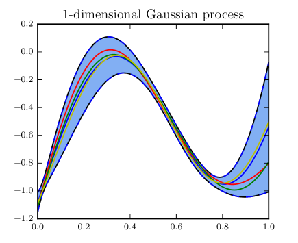
Fig. 1 shows an example of a one-dimensional Gaussian process. The dark blue line is the mean function of the process, the light blue region is the -region, and different color curves are samples from the process.
Gaussian process classification
Now we apply Gaussian processes to a binary classification problem. Suppose, we have a dataset , where , . Denote the matrix comprised of points by and the vector of corresponding class labels by . The task is to predict the class label at a new point .
We consider the following model. First we introduce a latent function and put a zero-mean GP prior over it:
for some covariance function . For now the covariance function is supposed to be fixed.
Then we consider the probability of the object belonging to positive class to be equal to for the chosen sigmoid function :
| (2) |
In this work we use the logistic function , however one could use other sigmoid functions as well.
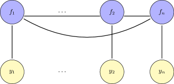
The probabilistic model for this setting is given by
| (3) |
where is sigmoid likelihood (2) and is GP prior. The corresponding probabilistic graphical model is given in fig. 2.
Now inference in the model (3) can be done in two steps. First, for new data point we should find the conditional distribution of the corresponding value of the latent process . This can be done as follows
| (4) |
Second, the probability that belongs to the positive class is obtained by marginalizing over the latent variable .
| (5) |
Unfortunately, both integrals (4) and (5) are intractable since they involve a product of sigmoid functions and normal distributions. Thus, we have to use some integral-approximation techniques to estimate the predictive distribution.
For example, one can use Laplace approximation method, which builds a Gaussian approximation to the true posterior . Substituting this Gaussian approximation back into (4) we obtain a tractable integral. The predictive distribution (5) remains intractable, but since this is a one-dimensional integral it can be easily estimated by quadratures or other techniques. The more detailed derivation of this algorithm and another algorithm, based on Expectation Propagation, can be found in [5].
Computational complexity of computing the predictive distribution both for the Laplace approximation method and Expectation propagation scales as since they both require to invert matrix . In section we describe the concept of inducing points aimed to reduce this complexity.
Model adaptation
In the previous section we described how to fit a Gaussian process to the data in the classification problem. However, we only considered Gaussian processes with fixed covariance functions. This model can be rather limiting.
Most of the popular covariance functions have a set of parameters, which we refer to as covariance (or kernel) hyper-parameters. For example, the squared exponential covariance function
has two parameters – variance and length-scale . An example of a more complicated popular covariance function is the Matern function, given by
with two positive parameters . Here is a modified Bessel function.
In order to get a good model for the data, one should find a good set of kernel hyper-parameters . Bayesian paradigm provides a way of tuning the kernel hyper-parameters of the GP-model through maximization of the model evidence (marginal likelihood), that is given by
| (6) |
However, this integral is intractable for the model (3) since it involves a product of sigmoid functions and normal distribution. In subsequent sections we describe several methods to construct a variational lower bound to the marginal likelihood. Maximizing this lower bound with respect to kernel hyper-parameters , one could fit the model to the data.
3 Variational inducing point GP-classification
In the previous section we showed how Gaussian processes can be applied to solve classification problems. The computational complexity of GP for classification scales as , that makes this method inapplicable to big data problems.
A number of approximate methods have been proposed in the literature for both GP-regression and GP-classification [8, 9, 10]. In this paper we consider methods based on the concept of inducing inputs. These methods construct an approximation based on the values of the process at some points. These points are referred to as inducing points. The idea is the following. The hidden Gaussian process corresponds to some smooth low-dimensional surface in . This surface can in fact be well approximated by another Gaussian process with properly chosen training points and process values at that points (inducing inputs). Then predictions of this new process at training points are used for constructing approximate posterior distribution for . The positions of inducing inputs can be learned within training procedure. However, for simplicity in the following we clusterize the dataset into clusters using K-means and choose to be cluster centres. In practice we observe that this approach works well in almost all the cases.
Evidence lower bound
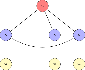
In the following we use a variational approach for solving maximum evidence problem (6). In this approach an evidence lower bound is introduced, that is simpler to compute than the evidence itself. Then this lower bound is maximized w.r.t. kernel hyperparameters and additional variational parameters used for constructing the lower bound.
Let’s consider the following augmented probabilistic model:
| (7) |
The graphical model for the model (7) is shown in fig. 3. Note that marginalizing the model (7) w.r.t gives the initial model (3).
We denote the covariance matrix comprised of pairwise values of the covariance function on the points by . Similarly, we define and .
As and are generated from the same Gaussian process with zero-mean prior,
| (8) |
where . In the following for simplicity we omit dependence on and in all formulas. Note that we do not consider optimization w.r.t. these values.
Applying the standard variational lower bound (see, for example [3]) to the augmented model (7), we obtain the following inequality:
for any distribution . This inequality becomes equality for the true posterior distribution . Next we restrict the variational distribution to be of the form
| (9) |
where for some , and is determined by (8). This is the key approximation step in inducing points approach for Gaussian processes. The chosen family (9) subsumes that with large enough all information about the hidden process values at training points can be successfully restored from the values at inducing inputs, i.e. .
The form (9) of the variational distribution implies a Gaussian marginal distribution
As depends on only through , the expectation
where is the marginal distribution of :
| (10) |
and is the -th column of matrix .
Finally,
Combining everything back together, we obtain the evidence lower bound
| (11) |
Note that the KL-divergence term in the lower bound (11) can be computed analytically since it is a KL-divergence between two normal distributions. In order to compute the expectations , we have to use integral approximating techniques.
The evidence lower bound (ELBO) (11) can be maximized with respect to variational parameters , and kernel hyper-parameters. Using the optimal distribution , we can perform predictions for new data point as follows
The last integral is tractable since both terms and are normal distributions.
SVI method
In case of classification we can’t analytically compute the expectations in the lower bound (11). However, the expectations are one-dimensional Gaussian integrals and can thus be effectively approximated with a range of techniques. In paper [2] Gauss-Hermite quadratures are used for this purpose. Note that the lower bound (11) has the form ”sum over training objects”. Hence this bound can be maximized using stochastic optimization techniques. Paper [2] suggests to maximize the lower bound (11) with respect to the variational parameters and kernel hyper-parameters using stochastic optimization. We refer to this method as svi method (abbreviation for Stochastic Variational Inference). The lower bound (11) and all it’s derivatives can be computed in . This complexity has a linear dependence on , hence svi method can be applied for the case of big training data.
1 Tractable evidence lower bound for GP-classification
In the previous section we described the svi method. It is based on stochastic optimization of the lower bound (11) for marginal likelihood and the lower bound itself is computed in . But the bound depends on parameters which makes the optimization problem hard to solve when a big number of inducing points is needed.
For GP-regression the situation is similar. Paper [1] describes a method analogical to the svi method for classification. The only difference is that the lower bound becomes tractable in case of regression. Then the paper [6] tries to solve the problem of big number of parameters in the algorithm from [1] in the following way. In case of regression the lower bound (11) can be analytically optimised with respect to variational parameters . Doing so and substituting the optimal values back into the lower bound, one can obtain a new lower bound to the marginal likelihood that depends solely on kernel hyper-parameters . This simplifies the optimization problem by dramatically reducing the number of optimization parameters. Unfortunately, this new bound doesn’t have a form of ”sum over objects”, hence stochastic optimization methods are no longer applicable here. However, in our experiments we’ve found that even for fairly big datasets the method from [6] outperforms [1] despite the lack of stochastic optimization.
In the following subsection we devise an approach similar to the method of [6] for the case of classification. We provide a tractable evidence lower bound and analytically maximize it with respect to variational parameters and . Substituting the optimal values of these parameters back into the lower bound we obtain a new lower bound, that depends only on kernel hyper-parameters .
Global evidence lower bound
In order to derive a tractable lower bound for (11), we seek a quadratic approximation to the log-logistic function , where . The paper [4] provides a global parametric quadratic lower bound for this function:
where and is a parameter of the bound. This bound is tight when .
Substituting this bound back to (11) with separate values for every data point, we obtain a tractable lower bound
where
Differentiating with respect to and and setting the derivatives to zero, we obtain
| (12) |
| (13) |
Substituting the optimal values of variational parameters back to the lower bound and omitting the terms not depending on and , we obtain a compact lower bound
| (14) |
where
In the following we consider three different methods for maximizing the lower bound .
Note, that given the values of , , , we can maximize with respect to analytically. The optimal values for are given by
| (15) |
The values and were defined in (10). In our first method we use analytical formulas (15) to recompute the values of and use gradient-based optimization to maximize the bound with respect to . The pseudocode is given in Alg. 1. We will refer to this method as vi-JJ, where JJ stands for Jaakkola and Jordan, the authors of [4]. Note that the computational complexity of one iteration of this method is , the same as for the svi method.
Our second method uses gradient-based optimization to maximize with respect to both and . Note that in this method we don’t have to recompute and at each iteration which makes the methods iterations empirically faster for big values of . We refer to this method as vi-JJ-full.
Finally, vi-JJ-hybrid is a combination of the two methods described above. The general scheme of this method is the same as vi-JJ. In the vi-JJ-hybrid method we use analytical formulas to recompute as we do in the vi-JJ method at stage , but at stage we use gradient-based optimization with respect to both and . The virtues of this method will be described in the experiments section.
Tractable local approximation to the evidence lower bound
Another way to obtain a tractable approximation to the lower bound (11) is to use a local quadratic approximation for the log-logistic function . In this way we perform a second-order Taylor expansion of this function at points :
| (16) |
The following derivation is analogical to the derivation in the previous section. Substituting the approximation (16) into the lower bound (11), we obtain
Here is a diagonal matrix
where .
Differentiating the approximate bound with respect to , , and , and setting the derivatives to zero, we obtain the following formulas for optimal values of these parameters:
| (17) |
| (18) |
Here
and is a vector, composed of
Substituting the optimal values for and , given by (17), (18), back into the approximate bound, and omiting the terms, that do not depend on , we obtain the following approximate lower bound:
| (19) |
where
Note that the lower bound (19) is not a global lower bound for the log-evidence . However, locally we get a good approximation of the evidence lower bound (11).
For maximizing the approximate lower bound (19) we consider a method, analogical to vi-JJ. In order to specify this method we simply substitute the bound by in the second stage in Alg. 1. We will refer to this method as vi-Taylor. The computational complexity of one iteration of this method is once again .
2 Experiments
In this section we empirically compare the derived vi-JJ, vi-Taylor, vi-JJ-full and vi-JJ-hybrid methods with svi. Below we describe the setting of the experiments and discuss their results.
Experimental setting
In our experiments we compared methods for variational inducing point GP-classification:
- •
-
•
vi-JJwas described in section ; -
•
vi-Taylorwas described in section ; -
•
vi-JJ-fullwas described in section ; -
•
vi-JJ-hybridwas described in section .
We also tried using deterministic L-BFGS-B optimization method for maximizing the evidence lower bound (11), but it worked substantially worse than all the other methods. Note, that all the methods have the same complexity of epochs . Table 1 shows which variables are optimized numerically and which are optimized analytically for each method.
| Method |
|
|
||||
|---|---|---|---|---|---|---|
svi-AdaDelta |
, , | |||||
vi-JJ, vi-Taylor
|
, , | |||||
vi-JJ-hybrid |
, | , , | ||||
vi-JJ-full |
, | , |
In our experiments we didn’t optimize the lower bound with respect to the positions of inducing points. Instead we used -means clustering procedure with equal to the number of inducing inputs and took clusters centres as . Also we used the squared exponential covariance function (see section Model adaptation) in all experiments with a Gaussian noise term.
The stochastic method svi-AdaDelta requires the user to manually specify the learning rate and the batch size for the optimization method. For the former we had to run the method with different learning rates and choose the value that resulted in the fastest convergence. We used the learning rates from a fixed grid with a step of . It always happened, that for the largest value from the grid the method diverged, and for the smallest the method converged slower, than for some medium value, verifying, that the optimal learning rate was somewhere in the range. To choose the batch size we used the following convention. For small german and svmguide datasets we’ve set the batch size to . For other datasets we used approximately as the batch size, where is the size of the training set.
For the vi-JJ, vi-Taylor and vi-JJ-hybrid in all of the experiments on every iteration we recomputed the values of , , and times ( in algorithm 1). To tune , on every iteration we’ve run L-BFGS-B optimization method constrained to do no more than evaluations of the lower bound and it’s gradient. We found that these values of parameters work well for all the datasets we experimented with.
For the svi-AdaDelta method we used optimization w.r.t. Cholesky factor of the matrix in order to maintain it’s positive definiteness, as described in [2]. We used AdaDelta optimization method implementation from the climin toolbox [7] as is done in the original paper.
For every dataset we experimented with a number of inducing points to verify that the results of the methods are close to optimal.
We evaluate the methods plotting the accuracy of their predictions on the test data against time. All of the plots have titles of the following format.
We also preprocessed all the datasets by normalizing the features setting the mean of all features to and the variance to . For datasets without available test data, we used of the data as a test set and as a train set.
Results and discussion
We compared the methods’ performance on seven datasets. Here we discuss the results.
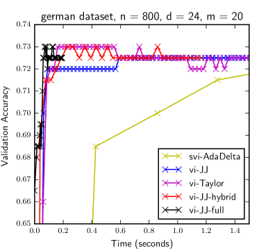
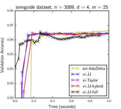
Fig. 4 provides the results for german and svmguide datasets. As we can see, on the small german dataset the stochastic svi-AdaDelta method struggles, and it takes it longer to achieve the optimal quality, than for all the other methods, which show similar results. On the svmguide dataset it takes vi-JJ-full and svi-AdaDelta a little bit longer to converge, while the other three methods show roughly the same performance.
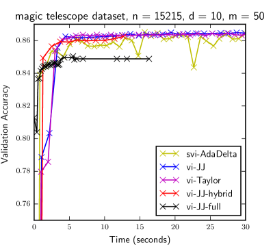
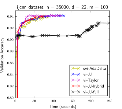
The results on magic telescope and ijcnn datasets are provided in fig. 5. On the magic telescope dataset the vi-JJ and vi-Taylor show poor quality on the first iterations, but still manage to converge faster, than svi-AdaDelta. On both datasets the vi-JJ-hybrid method works similar to vi-JJ and vi-Taylor, but shows better quality on first iterations on the magic telescope data. vi-JJ-full can’t converge to a reasonable quality on both datasets.
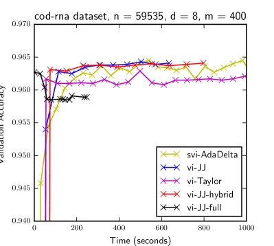
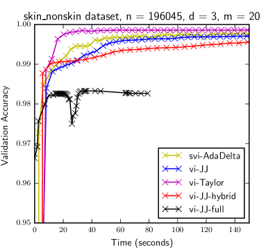
Fig. 6 provides the results on big cod-rna and skin_nonskin datasets. On these datasets the vi-JJ-full once again fails to achieve a reasonable quality, while the other methods work similarly.
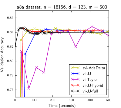
Finally, the results on a8a data are provided in fig. 7. Here we use a rather big amount of inducing inputs. As we can see, the vi-JJ-full and vi-JJ-hybrid are the fastest to achieve the optimal quality. The svi-AdaDelta method also converges reasonably fast, while the vi-JJ and vi-Taylor struggle a little bit.
In general vi-JJ, vi-Taylor and vi-JJ-hybrid methods perform similar to svi-AdaDelta method. On the big dataset skin_nonskin with only features the vi-JJ-hybrid is a little bit slower than the stochastic svi-AdaDelta, but on all the other datasets it is better. The vi-Taylor and vi-JJ struggle with a8a, but are otherwise comparable to vi-JJ-hybrid. The stochastic svi-AdaDelta method performs poorly on small datasets and even on the big skin_nonskin data doesn’t manage to substantially outperform the other methods, even provided a good value of learning rate. Finally, vi-JJ-full works well on small data and on the a8a, but on all the other datasets it doesn’t manage to achieve a reasonable quality.
3 Conclusion
In this paper we presented a new approach to training variational inducing input Gaussian process classification. We derived two new tractable evidence lower bounds and described several ways to maximize them. The resulting methods vi-JJ, vi-JJ-full, vi-JJ-hybrid and vi-Taylor are similar to the method of [6] for GP-regression.
We provided an experimental comparison of our methods with the current state-of-the-art method svi-AdaDelta of [2]. In our experimental setting, our approach proved to be more practical, as it converges to the optimal quality as fast as the svi-AdaDelta method without requiring the user to manually choose the parameters of the optimization method.
The four described vi methods showed similar performance and it’s hard to distinguish them. However, note that the vi-Taylor approach is more general and can be applied to the likelihood functions, that are not logistic. We could also easily derive a method, similar to vi-JJ-hybrid and vi-JJ-full for the non-logistic case, but it is out of scope of this paper.
References
- [1] J. Hensman, N. Fusi, and N. D. Lawrence. 2013. Gaussian processes for big data. Proceedings of the Twenty-Ninth Conference on Uncertainty in Artificial Intelligence. P. 282–290.
- [2] J. Hensman, G. Matthews, Z. Ghahramani. 2015. Scalable Variational Gaussian Process Classification. Proceedings of the Eighteenth International Conference on Artificial Intelligence and Statistics.
- [3] T. Jaakkola. 2000. Tutorial on Variational Approximation Methods. Advanced Mean Field Methods: Theory and Practice. P. 129–159.
- [4] T. Jaakkola, M. Jordan. 1997. A Variational Approach to Bayesian Logistic Regression Models and Their Extensions. Proceedings of the 1997 Conference on Artificial Intelligence and Statistics.
- [5] C. E. Rasmussen and C. K. I. Williams. 2006. Gaussian Processes for Machine Learning. MIT Press, Cambridge, MA.
- [6] M. Titsias. 2009. Variational learning of inducing variables in sparse Gaussian processes. Proceedings of the Twelfth International Workshop on Artificial Intelligence and Statistics. vol. 5, P. 567–574.
- [7] Climin. URL: http://github.com/BRML/climin.
- [8] A. Smola, P. Bartlett 2001. Sparse greedy Gaussian process regression. Neural Information Processing Systems.
- [9] J. Quinonero-Candela, C. Rasmussen 2005. A unifying view of sparse approximate Gaussian process regression. Journal of Machine Learning Research. vol. 6, P. 1939–1959.
- [10] L. Csato, M. Opper 2002. Sparse online Gaussian processes. Neural Computation. vol. 14, P. 641–668.