Constraints on dark matter scenarios from measurements of the galaxy luminosity function at high redshifts
Abstract
We use state-of-art measurements of the galaxy luminosity function (LF) at and to derive constraints on warm dark matter (WDM), late-forming dark matter (LFDM) and ultra-light axion dark matter (ULADM) models alternative to the cold dark matter (CDM) paradigm. To this purpose we have run a suite of high-resolution N-body simulations to accurately characterise the low-mass end of the halo mass function and derive DM model predictions of the high-z luminosity function. In order to convert halo masses into UV-magnitudes we introduce an empirical approach based on halo abundance matching which allows us to model the LF in terms of the amplitude and scatter of the ensemble average star formation rate halo mass relation, , of each DM model. We find that independent of the DM scenario the average SFR at fixed halo mass increases from to , while the scatter remains constant. At halo mass h-1 the average SFR as function of halo mass follows a double power law trend that is common to all models, while differences occur at smaller masses. In particular, we find that models with a suppressed low-mass halo abundance exhibit higher SFR compared to the CDM results. Thus, different DM models predict a different faint-end slope of the LF which causes the goodness-of-fit to vary within each DM scenario for different model parameters. Using deviance statistics we obtain a lower limit on the WDM thermal relic particle mass, keV at . In the case of LFDM models, the phase transition redshift parameter is bounded to at . We find ULADM best-fit models with axion mass eV to be well within of the deviance statistics. We remark that measurements at slightly favour a flattening of the LF at faint UV-magnitudes. This tends to prefer some of the non-CDM models in our simulation suite, although not at a statistically significant level to distinguish them from CDM.
I Introduction
In the past few years there has been significant progress in the characterization of the high-redshift UV-luminosity function (LF) (see e.g. Finkelstein2012 ; Bouwens2012 ; Oesch2013 ; Schenker2013 ; Mclure2013 ; Bouwens2015 ; Finkelstein2015 ; McLeod2015 ; Bouwens2016a ). Measurements from galaxy samples at have shown that the slope of LF remains steep to magnitudes (see e.g. Bouwens2015 ; Finkelstein2015 ) with important implications for scenarios of cosmic reionization. Evidence of such steepness persisting to very faint magnitudes () would imply the existence of a large population of dim galaxies contributing to the reionization of the universe (see e.g. Munoz2011 ; Jaacks2012 ; Cai2014 ; Mason2015 ). However, it is only very recently that observations have begun probing the galaxy LF at such low UV-luminosities. As an example, measurements of the LF to at and at have been obtained in Ishigaki2015 ; Atek2015a ; Atek2015b , while estimates to even fainter magnitudes have been obtained by Livermore, Finkelstein and Lotz Livermore2016 . The latter have been able to characterise for the first time the LF to at , at and at , showing that the LF slope remains steep to very faint magnitudes and at high-redshifts.
These measurements have been possible thanks to the detection of very faint high-redshift objects through the gravitational lensing magnification caused by massive galaxy clusters that are the targets of the Hubble Frontier Fields (HFF) program Coe2015 ; Lotz2016 . This novel approach is a promising alternative to deep galaxy survey searches such as the Hubble Ultra Deep Field Beckwith2006 ; Ellis2013 ; Illingworth2013 , but it is not exempt of systematic errors that can bias the determination of the LF. As an example, the uncertainty in the assumed size distribution of very faint galaxies Bouwens2016b and the magnification error due to lens model uncertainties can alter the LF faint-end slope Bouwens2016c . The latter has been shown to be the dominant source of systematics. In particular the analysis of Bouwens2016c has indicated that when carefully assessed, current LF estimates cannot exclude the presence of a flattening of the LF at the faint-end, as expected from a number of numerical simulations studies Jaacks2013 ; Oshea2015 , which would call into question some of the proposed reionization scenarios. However, the implications of these measurements are far wider than probing the link between galaxy formation models and cosmic reionization history, since they provide a test of the nature of dark matter (DM) itself.
In the standard cosmological model (e.g. Peebles1993 ), DM consists of cold, collisionless particles interacting with visible matter (and indeed other DM particles and neutrinos) only via gravity. This is known as the cold dark matter (CDM) paradigm, and has various motivations from particle physics such as supersymmetry, extra dimensions, axions, and string theory (for reviews, see e.g. Refs. 1996PhR…267..195J ; 2005PhR…405..279B ; 2016PhR…643….1M ). In such a scenario the faint galaxies observed at high-redshift populate small-mass DM halos. As an example, analytical models of the LF suggest that galaxies with magnitude at should be hosted in halos of mass of h-1 (see e.g. Munoz2011 ; Cai2014 ). Therefore, the recent measurements of the faint-end of the galaxy LF function at and probe the lightest and earliest to form DM objects, which are at the frontier of our knowledge.
The CDM paradigm has been tremendously successful at reproducing observations of the large-scale distribution of matter in the universe Spergel2003 ; Tegmark2004 ; Massey2007 ; Planck2015 . In contrast, the emergence of anomalies at small scales and the lack of detection of supersymmetric weakly interactive particles (WIMPs) or QCD axions in the lab (e.g. Refs. 2010PhRvL.104d1301A ; pdg ) have prompted the investigation of broader scenarios that evade detection in standard channels. For example, direct detection interpretations are altered when the DM production method breaks the link between thermal cross-section and abundance, when production is non-thermal, or when symmetry dictates particular couplings to be absent or suppressed. In the present work we will be particularly interested in models of DM that not only evade direct detection, but also differ from CDM in terms of cosmological structure formation, and as such can be probed with the high- LF. In these scenarios, astrophysics offers a probe of DM particle physics complementary to laboratory based searches.
We will consider three examples of DM models fitting this prescription. A warm dark matter (WDM) component with thermal relic particle mass , inspired by particle physics models of sterile neutrinos, has been advocated as a solution to the small-scale anomalies of CDM (see e.g. WDMth ; WDMph ). Sterile neutrinos in this mass range cannot be detected in standard WIMP searches at least with current experimental capabilities (see e.g. Liao2014 ; Mertens2015 ; Campos2016 ), but leave imprints on the cosmic structure formation due to their thermal velocities. Ultralight axions (ULAs) with mass may be present in hidden sectors, evading DM searches based on the couplings of the QCD axion 2006JHEP…06..051S ; 2010PhRvD..81l3530A ; 2016PhRvD..93b5027K . ULAs and other models of scalar field/wave DM affect structure formation due to their large de Broglie wavelength khlopov_scalar ; 1990PhRvL..64.1084P ; Sin1994 ; Lee1996 ; 2000PhRvL..85.1158H ; 2010PhRvD..82j3528M ; 2014MNRAS.437.2652M ; Schive2014 ; Hui2016 . Our third and final benchmark model is late-forming dark matter (LFDM) Das2011 ; Agarwal2015 . In such a scenario DM particles emerge from a scalar field undergoing a phase transition near matter-radiation equality which alters the small scale distribution of density fluctuations.111Other related scenarios that we do not consider include self-interacting DM (e.g. Refs. 2000PhRvL..84.3760S ; 2014PhRvD..89c5009K ), the “effective theory of structure formation” 2016PhRvD..93l3527C , and generalised models 1998ApJ…506..485H ; 2016PhRvD..94b3510K ; 2016PhRvD..94d3512K .
A common feature of these scenarios is the suppression of matter density fluctuations below a cut-off scale that depends on the specificity of the DM particle model. Traces of this signature have been tightly constrained using matter power spectrum measurements at from Lyman- forest observations (see e.g. Viel2013 ; Baur2016 ). However, it has been pointed out that such bounds may relax if the thermal evolution of the intergalactic medium is a non-monotonic function of redshift Garzilli2015 . A detailed discussion of other caveats pertaining the properties of the intergalactic medium that enter such analyses can be found in Hui2016 . Alternatively, DM models predicting a cut-off in the matter power spectrum can be constrained using measurements of the abundance of faint galaxies at high redshifts. This is because the suppression of power at small scale leads to suppressed abundance of low-mass halos. Similarly, constraints on DM scenarios can be inferred from measurements of the dark matter distribution in the local universe. Indeed, it was the discovery of small scale anomalies in the distribution of structures surrounding the Milky Way, such as the core-vs-cusp problem Moore1994 ; Kuzio2011 , the missing satellites problem Klypin1999 ; Moore1999 and the too-big-to-fail problem Boylan2011 ; Boylan2012 that have prompted the study of non-standard DM models such as WDM. Nevertheless, in the low redshift universe it is hard to disentangle whether such anomalies are the result of the non-standard properties of DM or the consequence of baryon feedback (see e.g. Libeskind2007 ; Maccio2010 ; Pontzen2012 ). This is because the amplitude and nature of the baryonic processes that contribute to the shaping distribution of matter at small scales and at late times remains largely uncertain (see e.g. Panarubia2012 ; Garrison2013 ). In the high-redshift universe on the other hand, baryonic processes are expected to be less complex, thus it is possible that measurements of the abundance of faint high-z galaxies hosted in low mass DM halos may provide more pristine insights on DM.
Constraints on the WDM models using earlier high-redshift LF measurements have already been obtained in numerous works in the literature. As an example, the authors of Pacucci2013 have derived constraints on WDM thermal relic mass from estimates of the high-redshift galaxy number density and found keV at . Using LF measurements at in combination with bounds on the optical depth parameter from Planck the authors of Lapi2015 found that keV. Strong exclusion bounds with keV at have been recently obtained in Menci2016 using the LF faint-end data from Livermore2016 . Differently from these analyses, the authors of Schultz2014 have obtained constraints on WDM models using high-redshift measurements of the cumulative luminosity function resulting in keV at .
A key assumption in the analysis of WDM models using LF measurements is the derivation of the relation between halo mass and UV-magnitude that is necessary to convert the N-body calibrated halo mass function into the LF model prediction. In Schultz2014 the authors have estimated this relation for the CDM model using halo abundance matching (HAM) and linearly extrapolated the relation to faint galaxy magnitudes. However, it is far from obvious that such a relation can be assumed to hold independent of the underlying DM model assumptions. For example, in Bozek2015 the authors have used a similar methodology to derive constraints on mixed axion-CDM models. However, unlike Schultz2014 , they calibrated halo mass and UV-magnitude relation for each of the investigated axion-CDM models. Instead of considering the cumulative LF, the authors of Schive2016 have used a conditional LF method to constrain wave dark matter models directly against LF measurements. Their analysis has found a lower bound on a boson-like DM particle mass, eV at .

Here, we aim to derive up-to-date bounds on several DM scenarios consisting of WDM, LFDM and ULADM, using a large compilation of high-redshift LF data. To this purpose we have run high-resolution N-body simulations which take as input modified initial conditions appropriate to each of the DM models considered. We accurately estimate the corresponding halo mass functions at low masses and at high-redshifts that we use to infer DM model predictions of the high-redshift luminosity function. As already stressed, this requires assuming a relation between halo mass and galaxy UV-luminosity. In order to improve upon the approaches of previous studies, we have developed a hybrid methodology (described in Section III) which intends to make progress in the use of LF measurements by addressing two important aspects previously overlooked: (i) it accounts for dust extinction on rest-frame UV photons which may alter the HAM inferred relation between halo mass and UV-magnitude at different redshifts. This is done by correcting the UV-luminosities using the established correlation between dust extinction and the UV-continuum slope Meurer1999 , and (ii) it allows us to gain insights on the DM model-dependence of the star formation rate (SFR) of high-redshift galaxies. This involves using the Kennicutt-relation Kennicutt1998 to convert the corrected UV LF measurements into SFR density functions (see e.g. Smit2012 ; Mason2015 ; Mashian2016 ).
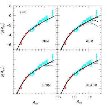
Our analysis of the high-redshift galaxy LF indicates that in the case of WDM models the thermal relic mass is constrained to be keV at (see Fig. 1 for a preview of the results at ). The same dataset excludes LFDM models with phase transition redshift at more than , while ULADM models with eV are compatible with the data within .
The paper is organised as follows: Section II describes the DM models, the N-body simulation characteristics and halo detection scheme. Section III details the hybrid method we use to model the high-redshift galaxy UV LF. The LF datasets used in this work are described in Section IV with the results presented in Section V. We discuss and conclude in Section VII.
II N-body simulations
In this section we describe the properties of the simulated DM models, the characteristics of the N-body simulations, the identification of halos and the evaluation of the halo mass functions.
II.1 Cosmological models
Our reference cosmological model is a standard flat cold dark matter model with cosmological constant (to which we will simply refer as CDM) specified by the following set of model parameters: matter density , baryon density , reduced Hubble parameter , scalar spectral index ,222After running the simulations of the CDM, WDM and LFDM models we realised that we had inadvertently generated the linear power spectrum of our reference CDM model with the scalar spectral index set to rather than the Planck best-fit value . Given the limited computing time allocation available to us we were unable to re-run these models, therefore we decided to complete the simulation suite with for the ULADM models as well. By using a larger value of our numerical simulations systematically predict slightly more power at small scales, resulting in a slight increase in the abundance of small-mass halos. This has the tendency to relax the constraints on the alternative DM models. Hence, we obtain more conservative bounds on the DM model parameters than what we would have inferred using . and root-mean-square fluctuation amplitude at . For this model we compute the linear matter power spectrum using the code camb Lewis2000 . The cosmological parameters listed above are common to all simulated models. We consider three classes of DM:
-
•
WDM models consisting of realizations with thermal relic particle mass keV (WDM-1), keV (WDM-2), keV (WDM-3), keV (WDM-4) and keV (WDM-5). The corresponding linear matter power spectra have been computed using the formulae provided in Bode2001 with the damping slope parameter set to and the number of degree-of-freedom .
-
•
LFDM models consisting of realizations with phase transition redshift (LFDM-1), (LFDM-2) and (LFDM-3). The linear power spectra of these models have been computed with a specifically modified version of camb (see Das2011 ).
-
•
ULADM models consisting of realizations with particle mass eV (ULADM-1), eV (ULADM-2) and eV (ULADM-3). We have computed the corresponding linear power spectra with the publicly available code axionCAMB333http://github.com/dgrin1/axionCAMB Hlozek2016 .
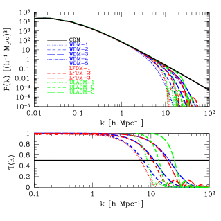
In the top panel of Fig. 2 we plot the linear matter power spectra of the simulated models at , while in the bottom panel we plot the transfer functions of the DM models with similar cut-off scale. We can see that the spectra converge to the reference CDM model on the large scales h Mpc-1, while differences arise in the suppression of power at smaller scales.
It is worth noticing that with our choice of model parameters, LFDM-1, LFDM-2 and LFDM-3, and ULADM-1, ULADM-2 and ULADM-3 are characterised by power spectra which have a cut-off scale nearly identical to that of WDM-2, WDM-3 and WDM-5 respectively. As can be seen in the bottom panel of Fig. 2, the corresponding transfer functions are also characterised by very similar half-modes444The half-mode is defined has the wavenumber at which the transfer function of a given DM model is half that of the corresponding CDM one 2016PhR…643….1M : (1) Notice that such a definition differs from that commonly used in the literature which defines as the wavenumber at which the power spectrum of a given DM model is half the value of the CDM one., these are quoted in Table 1. Despite such similarities, we can see that these models exhibit a different distribution of power for . Hence, it is reasonable to expect that this may lead to differences in the high-redshift abundance of small-mass halos for these models, a point which we discuss in detail in Section II.4.
| Model | Model | Model | |||
|---|---|---|---|---|---|
| WDM-2 | 7.3 | LFDM-1 | 6.6 | ULADM-1 | 8.7 |
| WDM-3 | 11.3 | LFDM-2 | 10.6 | ULADM-2 | 13.7 |
| WDM-5 | 20.4 | LFDM-3 | 18.8 | ULADM-3 | 25.2 |
II.2 Simulation characteristics
In principle, the use of N-body methods to simulate the non-linear structure formation of the non-standard DM cosmologies described above may not be a valid approach. This is because these models are characterised by microphysical processes that distinguish their particle dynamics from that of a purely collisionless DM component.
As an example, in the case of WDM models, one should in principle account for the distribution of thermal velocities Bode2001 ; Lowell2014 . This effect is usually implemented in numerical simulations as a random kick applied to the N-body particles (which trace the clustering of the matter density field), even though the root-mean-square velocity of WDM particles is several order of magnitudes smaller than that arising during the non-linear gravitational collapse. However, as pointed out in Angulo2013 , N-body particles are a coarse-grained representation of the phase-space distribution of the microscopic particles. Therefore the addition of a kick is equivalent to inducing a local coherent motion of a large ensemble of microscopic WDM particles, which leads to a velocity spectrum that is inconsistent with results from linear perturbation theory Colin2008 . In the case of fermionic WDM the Tremaine-Gunn effect Tremaine1979 leads to modified halo density profiles, however this occurs on scales smaller than those probed by the LF. Thus, as we are interested in deriving the mass distribution of DM halos, we can safely neglect this effect and run N-body simulations of WDM models with appropriate initial power spectra.
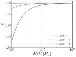
In the case of ULADM models, realistic simulations should solve the coupled Schrödinger-Poisson system (see e.g. Schive2014 ; Schwabe2016 or Veltmaat2016 for the particle in cell approach) to account for quantum wave-like effects that are specific to this class of models. However, as in the study by Schive et al. Schive2016 , the mass scales and redshifts which are of interest to our analysis are mostly insensitive to these effects. This is demonstrated in Fig. 3, where we plot the growth rate ratio, , defined in Schive2016 using the exact growth solution in 2016PhR…643….1M . As we can see, over the mass scale interval probed by LF observations the scale dependent growth rate of our lightest ULADM model differs from the CDM case by . Thus, for our purposes we can safely simulate the non-linear clustering of these models using the N-body method.
The use of N-body simulations is also justified in the case of the LFDM models, since in this scenario DM particles become collisionless soon after matter-radiation equality. Thus, by the initial redshift of the simulations the system becomes practically collisionless and its non-linear clustering can be followed through the dynamics of N-body particles with the appropriate initial power spectrum.
We run the code ramses Teyssier2002 to perform a series of high-resolution N-body simulations with the goal of resolving the low-mass end of the high-redshift halo mass function for the DM models described above. To this purpose we have simulated ( Mpc)3 volumes with particles corresponding to a particle mass resolution .
We generate initial conditions using the Zel’dovich approximation as implemented in mpgrafic Prunet2008 . For all models we use the same phase of the initial conditions and set the starting redshift of the simulations such that for a given model the standard deviation of the linear density field smoothed on the scale of the coarse grid is given by . Enforcing this constraint gives sufficiently high initial redshifts such as to guarantee that deviations from the Zel’dovich approximation remain negligible. For each model simulation we store eleven snapshots between and .
The simulations were run on the CURIE supercomputer of the Institute for Development and Resources in Intensive Scientific Computing (IDRIS) using 1024 processors for a total running time of 2 million hours.
II.3 Halo finder and spurious halo selection
We detect halos using a parallelised version of the friend-of-friend algorithm Davis1985 implemented in the code pFoF Roy2014 . This identifies halos as group of particles with a given linking length parameter , which we set to .
In order to reduce the impact of mass resolution errors, one may conservatively consider halos with at least 100 particles. However, in the case of cosmological models with suppressed spectra at small scales, the sampling of Poisson noise between the cut-off scale of the power spectrum and the Nyquist frequency of the simulations leads to the formation of spurious numerical halos, which cause an unphysical upturn of the halo mass function at low masses Gotz2002 ; Gotz2003 ; WangWhite2007 .
Several empirical methods have been investigated in the literature to identify and remove artificial halos. For instance, Wang & White WangWhite2007 have suggested to cut halo catalogs below a mass limit where is the mean matter density, is the mean intra-particle distance of the simulation, is the location of the peak in the dimensionless linear power spectrum and the numerical coefficient is estimated from simulations. A more sophisticated approach has been proposed in Lowell2014 , which relies on the idea that genuine proto-halos are spheroidal, thus spurious halos are identified as groups of particles associated to Lagrangian patches in the initial conditions characterised by a shape flatter than a certain threshold.
Here, we follow the approach presented in Agarwal2015 . This builds upon the fact that the structural properties of halos as described by the spin and shape parameters as well as the degree of relaxation provide distinct physical proxies of the genuine nature of halos in the simulations. In Agarwal2015 , the analysis of halo catalogs from WDM and LFDM simulations has shown that halos contributing to the upturn in the halo mass function are characterised by highly distorted statistical distributions of halo spin and shape parameters, which strongly correlate with large deviations from the virial condition as measured by the parameter ,555It is worth reminding that in the case of ULADM models the virial theorem is modified by the presence of the quantum pressure such that Schive2014b ; Hui2016 . This is not taken into account in our simulations, and we leave a detailed study to future work. where is the total kinetic energy of the halo particles and its gravitational potential energy.
As shown in Agarwal2015 , retaining halos with at least 300 particles and with deviations from the virial state in the range are sufficient conditions to remove the bulk of spurious objects from the numerical halo catalogs and recover undistorted statistical distributions for halo spin and shape parameters independently of the mass resolution of the simulations.
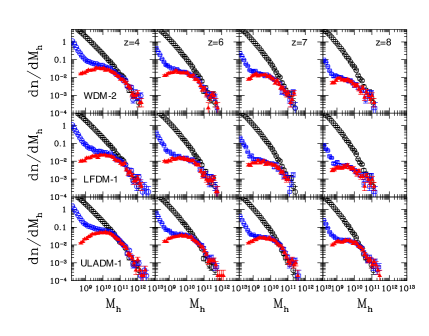
To illustrate the effect of spurious halos in our simulation suite we plot in Fig. 4 the halo mass function at and (panels from left to right) for WDM-2, LFDM-1 and ULADM-1 models (panels from top to bottom respectively). In each panel the black points represent the CDM mass function, while blue (red) points denote the non-standard DM model mass function before (after) spurious halo selection. Error-bars are given by the Poisson error within each mass bin. For each model we can see that at the high-mass end the mass function converges to that of CDM. This is expected, since on large scales the models have linear matter power spectra identical to that of the CDM case. At low masses () we can see the characteristic upturn which is indicative of the presence of spurious halos. In particular, the lower the redshift the higher the amplitude of the upturn, consistent with the expectation that the number of spurious halos increases as the simulation evolves from earlier to later times. After halo selection, the upturn disappears and we recover the expected halo abundance suppression at the low-mass end.
We apply the selection criteria of Agarwal2015 to all numerical halo catalogs. Since we consider halos with no less than 300 particles, the selected halo catalogs have a mass cut at M. Therefore, with the intent of being as conservative as possible we will not extrapolate any result below .
II.4 Halo mass function
| z | A | a | p |
|---|---|---|---|
| 4 | 0.35620 | 0.94020 | -0.87256 |
| 5 | 0.29542 | 0.94630 | -0.99538 |
| 6 | 0.29188 | 0.82990 | -0.84125 |
| 7 | 0.21785 | 0.91178 | -1.1072 |
| 8 | 0.25823 | 0.79364 | -0.81431 |
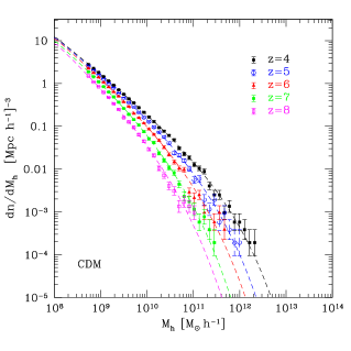
We fit the halo mass function of the CDM model as:
| (2) |
where is the mean matter density, is the root-mean-square of the linear density field smoothed on the scale enclosing a spherical volume of mass , and is the Sheth-Tormen (ST) multiplicity function Sheth1999 :
| (3) |
where with being the linear spherical collapse threshold computed using the formula given in Kitayama1996 . We determine the best-fit ST coefficients using a Levenberg-Marquardt minimisation scheme. These are quoted in Table 2 for the redshifts of interest. In Fig. 5 we plot the numerical mass functions against the ST best-fits.
We use the CDM calibrated formula to fit the mass function of the non-standard DM simulations using the following parameterisation:
| (4) |
where , , and are parameters which we best-fit against the N-body mass function. We prefer to work with such a parameterisation rather than the formula introduced in Angulo2013 , since it provides better fits to the numerical data. Accordingly, we find the best-fit functions to have reduced . In Appendix A we illustrate the goodness-of-fit of Eq. (4) and quote the values of the best-fit coefficients for all simulated DM models.666In order to avoid confusion we want to remark that the identification of as a mass scale cut-off related to a DM model parameter such as the thermal relic mass in the case of WDM models or the axion mass in the case of ULADM models is valid only for . Since we find for all models, one should not associate any particular physical meaning to the redshift evolution of the best-fit values of quoted in Tables 8, 9 and 10.

As discussed in Section II.2 the models LFDM-1, LFDM-2 and LFDM-3, and ULADM-1, ULADM-2 and ULADM-3 are characterised by a power spectrum cut-off which is nearly identical to that WDM-2, WDM-3 and WDM-5 respectively. Nevertheless, we find differences among these models for the predicted abundance of low-mass halos at high-redshifts which are well above the numerical statistical uncertainties ( level). This can be seen in Fig. 6, where we plot the ratio of the best-fit mass function at and (left to right panels) for WDM-2/LFDM-1 and WDM-2/ULADM-1 (top panels), WDM-3/LFDM-2 and WDM-3/ULADM-2 (central panels), and WDM-5/LFDM-3 and WDM-5/ULADM-3 (bottom panels). Ratios with respect to the LFDM models are shown as red dotted lines, while those with respect to ULADM models are shown as blue solid lines. In particular, we can see that the WDM models have systematically greater abundances of low-mass halos relative to the LFDM counterparts, while the opposite occurs for the ULADM modes. As can be seen in the lower panel of Fig. 2, this is consistent with the fact that the LFDM models have transfer functions that for are systematically lower than the WDM ones, while the ULADM transfer functions are larger. We will see that these differences manifest in different predictions of the faint-end slope of the LF at high-redshifts.
III Methodology
Our goal is to constrain the simulated DM models using an up-to-date compilation of high-redshift LF data at and covering an unprecedented UV-magnitude range from the brightest to the very faint. In order to convert the N-body calibrated mass functions into LF model predictions that can be compared to the data it is necessary to specify a relation between halo mass and UV-luminosity. As already mentioned in Section I, past studies in the literature computed such a relation using HAM methods Schultz2014 ; Bozek2015 or assumed a parametric form to be constrained by the LF data Schive2016 .
Here, we adopt a hybrid method with the intent of gaining insight on the evolution of the star formation rate of high-redshift galaxies as a function of redshift and host halo mass, as well as assessing the impact of dust extinction on the rest-frame UV-luminosities. The approach used here can be summarized as follows:
-
•
LF measurements are corrected for dust extinction using the established relation between extinction and UV-continuum slope from Meurer1999 . In particular, we calibrate an extinction model using UV-continuum slope measurements from Bouwens et al. Bouwens2014 to correct LF data at and from Bouwens2015 . The implementation of this extinction correction is described in Section III.1;
-
•
the corrected LF data at and is converted into the respective SFR densities using the Kennicutt-relation Kennicutt1998 .
-
•
The inferred functions at and , together with the halo mass function fits to the N-body simulations, are used to derive relation using HAM technique. The relations at and are then redshift-averaged to obtain the average relation, . This is repeated for each of the simulated DM model. This step is described in Section III.2;
-
•
For each DM model, after converting the SFR back into UV-luminosities we model the LF at and by integrating over the halo mass function a log-normal SFR probability density distribution with average and intrinsic dispersion , where and are free parameters. This will be explained in detail in Section III.3;
-
•
Finally, a -analysis of LF data at and is performed to determine the best-fit values of and , and evaluate the goodness-of-fit for each DM model.
To avoid confusion, hereafter we refer to density function as to denote , and as to denote , where is the cumulative density function.
III.1 Dust extinction correction & SFR densities
We correct the LF data using the empirical relation between extinction and UV-continuum slope, Meurer1999 . Following Smit2012 , at each we assume to be normal distributed with mean and dispersion , giving the average extinction . is set to zero when .
We model the mean slope as in Trenti2015 ; Mason2015 :
| (5) |
where and . We approximate and as linear redshift functions with coefficients determined by least-square interpolation of the values given in Table 3 of Bouwens2014 . This gives:
| (6) |
The extinction correction has a twofold effect on the LF function (see e.g. Smit2012 ). First, it shifts the LF toward brighter magnitudes since
| (7) |
where . Second, it alters the magnitude bin-size and consequently the amplitude of the LF. Denoting with the bin-size of the uncorrected LF, we have
| (8) | |||||
Thus the corrected LF reads as
| (9) |
We use Eq. (7) and Eq. (9) to correct the LF measurements (including errors) from Bouwens et al. Bouwens2015 at and . These are displayed in Fig. 7, where we plot the LF data (including errorbars) at (red points) and (blue points) before (filled circles) and after (empty triangles) correction for dust extinction.

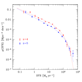
We convert the corrected LFs into SFR densities using the Kennicutt-relation 777Absolute magnitudes and luminosities in cgs units are related as: (10) Kennicutt1998 . We fit the SFR density estimates with a Schechter fitting function:
| (11) |
The best-fit values of , and at and are quoted in Table 3, while in Fig. 8 we plot the SFR density function measurements against the best-fit Schechter functions.
| z | [Mpc-3 dex-1] | SFR∗ [M⊙ yr-1] | |
|---|---|---|---|
| 4 | 0.49055E-03 | -0.16551E+01 | 0.46798E+02 |
| 5 | 0.29502E-03 | -0.16995E+01 | 0.47624E+02 |
III.2 Average -SFR relation
We use the analytical fits to the SFR density functions and the halo mass functions to compute the relation at and from halo abundance matching, (see e.g. Mashian2016 ), for each DM model in our simulation suite. The inferred relations are shown in Fig. 9 for the CDM (top left panel), WDM (top right panel), LFDM (bottom left panel) and ULADM (bottom right panel). The horizontal dotted lines indicate the limiting values of SFR covered by the extinction corrected LF measurements Bouwens2015 .
Let us focus on the CDM case. We can see that in the range covered by the LF observations the values of SFR at and span three orders of magnitude, yet the difference in SFR at fixed halo mass between and does not exceed a factor of across the entire mass range. The largest differences occur at the high and low-mass ends. At both redshifts the curve exhibit a change of slope at M, with a steep power law behaviour for and a flatter trend for . This is consistent with the findings of Mashian2016 , where the authors have pointed out that the steep slope at low masses can be indicative of feedback mechanisms that inhibit star formation.


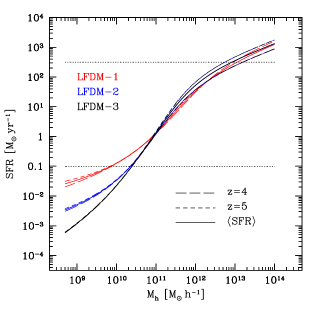

However, from Fig. 9 we can see that such interpretation only holds for the CDM scenario. In fact, for WDM, LFDM and ULADM models we find a systematic deviation from the CDM trend at low masses. Only at large masses, M all models converge to the same SFR-Mh relation at both redshifts. Notice that such deviations correlate with the level of suppression of the low-mass halo abundance compared to the CDM model. For instance, in the case of WDM-1 the SFR in halos of mass M is up to a factor larger than CDM, while in the case of WDM-2 the SFR is a factor larger. This follows from the imposed equality of the number density distributions in halo mass and SFR. In other words, DM models with suppressed halo mass abundance at fixed low mass need a larger star formation rate to match the observed SFR densities compared to the CDM prediction. The end result is that in the alternative DM scenarios the star formation rate halo mass relation tends to flatten at the low mass end compared to CDM model. This implies that in such alternative DM scenarios, in order to reproduce LF observations, feedback mechanisms must operate differently than in CDM, being either less efficient in suppressing star formation or even promoting it depending on the specificities of DM model considered. The plots shown in Fig. 9 also suggest that LF independent measurements of the SFR and host halo mass in galaxies at and can directly test these trends and put constraints on the DM scenario.
An important point that we would like to emphasise is the fact that the shape of the remains mostly unaltered between and , which corresponds to a time scale of Myr. In particular, the differences between the two curves can be accounted to good approximation by an overall amplitude factor. Thus, for each DM model, we derive a template form of the relation, , by averaging the HAM inferred relation at and at fixed halo mass. We use this template function to model the ensemble average star formation rate mass relation at and . This is similar in spirit to the LF model calibration by Mason, Trenti & Treu Mason2015 who have performed HAM against LF data at from Bouwens2015 to calibrate a redshift independent star formation efficiency. In our case, we assume that the ensemble average star formation rate differs from the calibrated template at and by an unknown constant amplitude factor.
This ansatz has a twofold aspect. First, it implies that the shape of over the mass range of interest is set by physical mechanisms very early on at redshift higher than . Secondly, since and differ by approximately Myr, the assumption of a constant scaling in amplitude is equivalent to assuming that there are no feedback processes (e.g. supernova explosions) that in such a time scale can significantly alter the shape of the average relation in the mass range of interest.
III.3 Modelling of high- luminosity function
We model the galaxy LF at as in Mashian et al. Mashian2016 and assume that the probability of having a galaxy with star formation rate SFR in a halo of mass Mh (i.e. the conditional SFR density) is given by a log-normal distribution. However, differently from Mashian2016 we assume the mean888We denote as the ensemble average of the SFR at fixed halo mass and redshift . to be given by with variance :
| (12) |
where is the template relation previously computed for each DM model, is a free parameter accounting for the overall amplitude of the relation at redshift and is a free parameter which accounts for the intrinsic scatter around this relation. The latter parametrises the stochasticity of the processes which are responsible for the star formation.
We compute the SFR density at a given redshift by integrating Eq. (12) over the halo mass function of a given DM model:
| (13) |
then using the Kennicutt-relation we convert SFR into UV-magnitudes to derive the extinction-free LF function in terms of the SFR density999For clarity, we have where in the last term we have used the Kennicutt-relation and the magnitude-luminosity relation. ,
| (14) |
Finally, using Eq. (9) to transform dust-free UV-magnitudes into the observed ones, , we obtain the DM model prediction of the LF with and as free parameters of the model.
At this point it is worth reminding the reader of the differences between the approach described above and the evaluation of the high-z LF presented in Mashian2016 and Schive2016 . In Mashian2016 , the ensemble average is derived by averaging at fixed halo mass the relation inferred from halo abundance matching using SFR densities estimates from LF measurements at . Moreover, they set a redshift-independent intrinsic scatter to dex. In contrast, in Schive2016 the authors have modelled the conditional luminosity function as a log-normal distribution and assumed a parametric form of the average UV-luminosity halo mass relation (with three fitting model parameters) and a free dispersion parameter inspired by the conditional LF model of Cooray2005 .
Our approach takes advantage of both methods in that the ensemble average star formation halo mass relation is modelled in terms of a template function (rather than a parametric one) determined from LF data at (rather than averaging across a larger redshift interval) with the LF prediction depending only on two free model parameters.
IV Data Analysis
IV.1 Luminosity function datasets
Over the past few years several groups have measured the galaxy luminosity function at (see e.g. Mclure2013 ; Schenker2013 ; Bouwens2015 ; Finkelstein2015 ). These studies have been able to precisely characterise the bright-end of the LF (), while only recently it has been possible to probe the faint-end thanks to the detection of faint distant objects lensed by massive clusters observed in the context of Hubble Frontier Fields program Atek2015b ; Livermore2016 ; Bouwens2016c .
Bouwens et al. Bouwens2015 (B15 hereafter) have characterised the luminosity function at using the largest galaxy sample to date from HST data. In Section III.2 we have used their LF measurements at and to calibrate our SFR-Mh template. We use their LF estimates at and (see Table 5 in B15) to infer constraints on the simulated DM models.
Previous estimate of the LF in the same magnitude range at and were obtained by Schenker et al. Schenker2013 and McLure et al. Mclure2013 . However, these analyses use smaller galaxy samples than those of B15. Moreover, their estimates of the total magnitude of galaxies assume them to be point sources, which as shown in the analysis presented in the Appendix G of Bouwens2015 introduces a systematic bias in the UV-magnitude determination of the most luminous and extended sources. For these reasons we do not include the LF measurements from Schenker2013 ; Mclure2013 in our analysis.
Luminosity function measurements over the same redshifts and UV-magnitude intervals of B15 have been obtained independently by Finkelstein et al. Finkelstein2015 . The galaxy samples used in the latter work largely overlap with those of B15. However, this analysis uses different selection criteria and data reduction procedures which may be responsible for the slight underabundance of bright galaxies compared to the findings of B15.
The dust extinction model parameters used in our analysis have been calibrated to the values inferred from Bouwens2014 which uses galaxy samples (and data reduction procedures) that are common to those used in B15. Furthermore, the effect of the extinction is more important on the bright-end of the LF. Hence, for coherence we discard the LF data from Finkelstein et al. Finkelstein2015 and only use the B15 data to cover the bright-end interval of the LF.
Measurements of the bright-end LF at and have also been obtained by Willott et al. Willott2013 and Ouchi et al. Ouchi2009 respectively. More recently Bowler et al. Bowler2014 ; Bowler2015 ; Bowler2017 have derived LF estimates at these redshifts in the magnitude range , which in combination with the B15 data at and better anchor the bright-end LF slope. However, we have verified that the use of these additional datasets does not lead to further constraints on the DM model fits, since these only affect the faint-end of the LF.
LF measurements to have been obtained by Atek et al. (Atek2015b , A15 hereafter) using a sample of galaxy candidates at and candidates at detected through HST observations of A2744, MACS 0416 and MACS 0717 clusters from the HFF program. More recently Livermore, Finkelstein & Lotz (Livermore2016 , L16 hereafter) have obtained LF measurements to at , at and at using a sample of galaxies detected through the analysis of A2744 and MACS 0416 clusters in HFF and including sources that escaped detection in A15.
As mentioned in Section I these observations have opened the way to a new alternative approach to explore the population of faint sources in the far distant universe. However, differently from deep survey searches, these LF estimates may be affected by a number of systematic errors that need to be carefully evaluated. As pointed out by Bouwens et al. (Bouwens2016c , hereafter B16), lens mass model uncertainties affect the evaluation of the magnification of the faintest sources and introduce a systematic bias in the characterisation of the LF. In B16, the authors have introduced a methodology to incorporate this effect in the determination of the LF. Using a sample of galaxies detected through observations of Abell 2744, MACS 0416, MACS 0717 and MAC 1149 they inferred the LF at .
| Dataset | |||
|---|---|---|---|
| B15 Bouwens2015 | |||
| A15 Atek2015b | - | ||
| L16 Livermore2016 | |||
| B16 Bouwens2016c | - | - |
As a consistency check, we fit the various LF data with the Schechter-function:
| (15) |
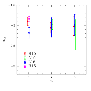
where is a normalisation parameter, an exponential cut-off scale and the faint-end slope, and run a Markov Chain Monte Carlo (MCMC) likelihood analysis to infer constraints on the Schechter parameters for the B15, A15, L16 and B16 datasets . We refer the reader to Section IV.2 for a general description of the statistical approach adopted here. Since constraints on the different DM models are sensitive to the faint-end slope, we do not compare constraints on and across the datasets and limit our consistency test to .
In Table 4 we quote the marginalised mean and error on . Notice that the mean values given in A15, L16, and B16 are slightly different from those quoted in Table 4. More importantly our estimated errors on are larger. This is because differently from the original analyses we do not combine the datasets with additional LF measurements covering the bright-end of the luminosity function.
In Fig. 10 we plot the values quoted in Table 4 for B15 (red solid circles), A15 (green solid triangles), L16 (blue empty circles), B16 (magenta empty squares). We can see that the bounds on at from L16 do not overlap with those obtained using B15 measurements. In contrast, the LF measurements from B16, which have been obtained by accounting for the lens mass model uncertainties, give bounds that are consistent with those obtained from the fit to B15. Similarly, at and the values of from B15, A15 and L16 are compatible with each other to within .
In the light of these results, we consider a compilation of LF data consisting of measurements (B15+B16) at , measurements (B15+A15+L16) at and measurements (B15+A15+L16) at spanning the UV-magnitude interval , while in a separate analysis we evaluate the impact of the L16 measurements at on the DM models.
| Model | ||||||||||
| CDM | 21.5 | 27.6 | 15.8 | 64.9 | ||||||
| WDM-1 | 87.7 | 57.4 | 23.8 | 168.9 | ||||||
| WDM-2 | 22.4 | 31.6 | 17.5 | 71.5 | ||||||
| WDM-3 | 20.5 | 28.1 | 15.7 | 64.3 | ||||||
| WDM-4 | 21.7 | 27.8 | 15.9 | 65.4 | ||||||
| WDM-5 | 22.0 | 27.1 | 15.8 | 64.9 | ||||||
| LFDM-1 | 37.2 | 45.0 | 16.6 | 98.8 | ||||||
| LFDM-2 | 20.1 | 28.3 | 15.6 | 64.0 | ||||||
| LFDM-3 | 21.7 | 30.5 | 16.2 | 68.4 | ||||||
| ULADM-1 | 21.3 | 33.6 | 14.9 | 69.8 | ||||||
| ULADM-2 | 21.5 | 31.4 | 16.5 | 69.4 | ||||||
| ULADM-3 | 21.9 | 27.3 | 15.9 | 65.1 |
IV.2 Likelihood Evaluation
We perform a Markov Chain Monte Carlo (MCMC) likelihood data analysis to derive constraints on the parameters characterising the theoretical LF model . To this purpose we evaluate the following :
| (16) |
where are the LF measured values. Since no information is available concerning possible correlations among different UV-magnitude bins, for simplicity we assume all LF measurements to be statistically independent.
We generate the random chains using a Metropolis-Hastings algorithm. We evaluate the rejection rate every 100 steps and adjust the width of the parameters dynamically. We set uniform priors for the LF model parameters.
For the Schechter-fitting function analysis described above, we have computed the with given by Eq. (15) and sampled a 3-dimensional parameter space with uniformly varying in the range , and respectively. For the DM model analysis, we have computed the with given by Eq. (14) (after having converted the dust-free UV-magnitude into observed ones) and sampled the 2-dimensional parameter space with uniformly varying in the range . For each model we run 3 independent chains of samples and check their convergence using the Gelman-Rubin test Gelman1992 .
V Results
Here we present the results of the likelihood data analysis. We first focus on the goodness-of-fit of the different DM models and derive constraints on a given DM scenario using deviance statistics. Then we discuss the constraints on the parameters of the SFR-Mh relation for the best-fit DM models.
V.1 DM models goodness-of-fit
In Table 5 we quote the best-fit LF model parameters and the corresponding -values at and for each of the simulated DM models, while in Fig. 11 we plot the corresponding LF against the data.
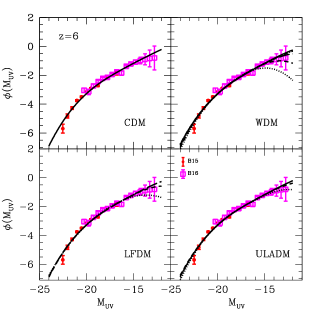

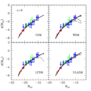
We find that the CDM model provides a very good fit to the LF data with total reduced chi-square . Among the alternative DM models, we find WDM-3, LFDM-2 and ULADM-3 to be those with the lowest . These are comparable or even slightly lower than that of the CDM model with differences . Thus, given current LF measurements, these models are statistically indistinguishable from the standard CDM scenario. On the other hand, we can see that varies from one model to another within each DM scenario.
The deviance statistics indicate that the best-fit WDM-1 model is excluded at more than compared to the best-fit WDM-3 model with , WDM-2 is excluded at more than with ( probability), while WDM-4 and WDM-5 are statistically compatible within ( probability). Thus, we infer a bound on thermal relic particle mass keV at . Similarly, in the LFDM case we find that LFDM-1 is excluded at more than with respect to LFDM-2 with , while LFDM-3 lies within with . This suggests that for LFDM models, the phase transition redshift at . The best-fit models of ULADM-1 and ULADM-2 are within of ULADM-3 with differences . Thus, ultra-light axion models with are compatible with the LF data well within of the deviance statistics.
It is worth noticing that the LF data at shows a slight preference (though not statistically significant) for DM models with a flattening of the faint-end slope. This is consistent with the results of B16 where the authors pointed out that the faint-end LF measurements at permit a turnover (within ) at . At higher redshifts LF data do not cover such faint magnitude interval and have much larger statistical uncertainties, thus the presence of a turnover or a flattening in the LF remains largely uncertain. In the context of the standard CDM scenario, the flattening of LF at the faint-end and the presence of a turnover can be the signatures of physical processes affecting star formation in low-mass galaxies as found in numerical studies based on hydrodynamical simulations Jaacks2013 ; Oshea2015 ; Wise2014 and semi-analytic models of galaxy formation Liu2016 . From Fig. 11 we can clearly see that such a feature is also a distinct prediction of DM models alternative to the CDM paradigm.

V.2 Constraints on SFR-Mh relation
We compute the average and marginalised errors on and from the MCMC chains. The values for the various DM models at and are quoted in Table 6. We find the parameter posteriors to be well approximated by a Gaussian distribution. This can be inferred from the fact that the best-fit LF parameter values given in Table 5 coincide to good approximation with average ones. As an example, this can also be seen in Fig. 12 where we show the triangle plot of the one and two-dimensional distributions of and for the CDM model at . Similar results hold for all models and at all redshifts.
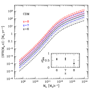
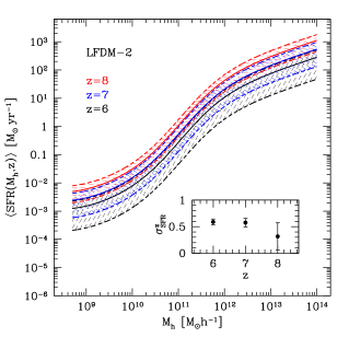
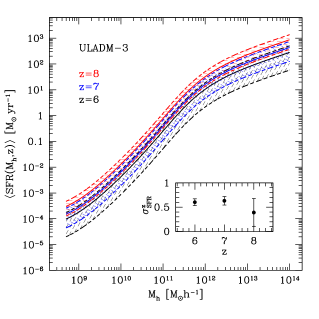
From the values quoted in Table 6 we can see that the values of and at a fixed redshift do not vary significantly among the different DM models. On the other hand, we find evidence of a systematic increase of from to , while the scatter remains constant. We can see this more clearly in Fig. 13 where we plot at (black lines), (blue lines) and (red lines) for CDM (top left panel), WDM-3 (top right panel), LFDM-2 (bottom left panel) and ULADM-3 (bottom right panel). The solid lines represent the ensemble average star formation halo mass relation with amplitude factor given by the marginal mean value quoted in Table 6. The dashed lines indicate the statistical error. In each panel we also plot the marginal mean of the intrinsic scatter and the related uncertainty.
| Model | ||||||
|---|---|---|---|---|---|---|
| CDM | ||||||
| WDM-1 | ||||||
| WDM-2 | ||||||
| WDM-3 | ||||||
| WDM-4 | ||||||
| WDM-5 | ||||||
| LFDM-1 | ||||||
| LFDM-2 | ||||||
| LFDM-3 | ||||||
| ULADM-1 | ||||||
| ULADM-2 | ||||||
| ULADM-3 |
For DM models with lowest , we find the intrinsic scatter dex which is consistent with the value assumed in Mashian2016 .
We may notice that all models exhibit the same power law trend at high masses, M, while differences occur at lower masses. In particular, we notice a broken power law behaviour at the low-mass end for the WDM-5, LFDM-3 and ULADM-3 models, which have higher SFR at fixed halo mass than the CDM case. This is consistent with the conclusion of the study on early galaxy formation in the WDM scenario presented in Dayal2015 and based on semi-analytical models (see also Kang2013 ). As already stressed in Section III.2, the differences at low masses imply that in non-standard DM models the baryonic processes that regulate star formation during early galaxy formation must operate differently than in CDM. More precisely, the curves shown in Fig. 13 represent constraints that simulations including baryonic physics in such alternative DM models need to reproduce to be compatible with LF observations. This will be worth investigating in the future using DM+hydro simulations.

VI Implications of Livermore et al. Livermore2016 data at
Here, we discuss how the LF data at from L16 modify the constraints on the DM models inferred in the previous section. Since, these measurements points to a steeper faint-end slope of the LF, we may expect the constraints on the DM scenarios to favorite models with a SFR-Mh relation closer to that of the CDM case. In Table 7 we quote the of the DM models best-fitting the LF data at (L16+B15 for a total 23 data points), while in Fig. 14 we plot the corresponding best-fit luminosity functions. Not surprisingly the models with the lowest values are those with the lest suppression of halo abundance at low masses.
However, it is worth noticing that none of the models provide a good fit to the LF data, since the reduced . This may point to the fact that the L16 data at requires a shallower slope of the SFR-Mh at low masses than that inferred from the LF data at and , which is not the case at and . We find WDM-5, LFDM-2 and ULADM-3 to be the models with the lowest values with respect to the realisations of the same DM scenario.
The deviance statistics indicates that the best-fit WDM-1 model is excluded at more than with , WDM-2 is excluded at more than with . while WDM-3 has . This suggests a lower bound on the WDM thermal relic mass corresponding to keV. This is slightly stronger than that inferred using the Bouwens et al. data at . In the case of LFDM models, the deviance statistics exclude the best-fit LFDM-1 model to more than with , while LFDM-2 and LFDM-3 are within of each other. This corresponds a constraint on similar to the inferred in Section V. On the other hand for the ultra-light axion models we find that ULADM-1 and ULADM-2 are excluded at more than with and respectively. This points to a strong bound on the axion mass eV at , which is consistent with the constraints found in Menci2017 using the galaxy number density estimated from L16 at .
| Model | ||
|---|---|---|
| CDM | 47.1 | 90.5 |
| WDM-1 | 98.2 | 179.4 |
| WDM-2 | 53.4 | 102.5 |
| WDM-3 | 48.6 | 92.4 |
| WDM-4 | 47.0 | 90.7 |
| WDM-5 | 46.3 | 89.2 |
| LFDM-1 | 67.8 | 129.4 |
| LFDM-2 | 49.5 | 93.4 |
| LFDM-3 | 47.2 | 93.9 |
| ULADM-1 | 59.8 | 108.3 |
| ULADM-2 | 46.8 | 94.7 |
| ULADM-3 | 46.6 | 89.8 |
VII Conclusions
Measurement of the faint-end of the galaxy luminosity function at high redshifts is key to understanding the connection between early galaxy formation and scenarios of cosmic reionization. Moreover, by probing the abundance of far distant galaxies hosted in the lightest DM halos, one can also potentially test the nature of dark matter particles in the universe. Scenarios alternative to the CDM paradigm have been investigated in recent years in response to the lack of detection of weakly interacting massive particles in laboratory experiments and as a possible solution to anomalies in the observed distribution of matter at small scales.
Using up-to-date measurements of the high-redshift galaxy luminosity function we infer constraints on DM scenarios alternative to CDM that feature a small scale cut-off in the linear matter power spectrum. To this purpose we have run a series of high-resolution N-body simulations of warm dark matter, late-forming dark matter and ultra-light axion dark matter models to accurately characterise the low-mass end of the halo mass function at high redshifts ().
We have removed artificial groups of particles from the N-body halo catalogs using a selection criterion based on the analysis of the structural properties of the halos. We have used the resulting halo catalogs to calibrate analytical formula of the halo mass function which we have utilised to infer DM model predictions of the high-redshift galaxy luminosity function.
In order to convert halo masses into UV-magnitudes we have developed an empirical approach based on halo abundance matching that has a twofold advantage: (i) it accounts for the effect of dust extinction which may alter the redshift dependence of the UV-magnitude halo mass relation, and (ii) it allows us to gain insight on the star formation rate of galaxies as a function of host halo mass and redshift.
Using a compilation of state-of-art measurements of the LF at and we perform a likelihood analysis to evaluate the goodness-of-fit of the simulated DM models and infer constraints on the amplitude and scatter of the ensemble average SFR-Mh relation in such models.
We find that at fixed halo mass the average SFR slightly increases with increasing redshift, while the scatter remains constant. For all DM models considered, the SFR-Mh relation converges to the double power law behaviour of the CDM model at h-1, while differences occur at lower masses. In particular, DM models characterised by a suppression of low-mass halo abundance exhibit systematically higher SFR compared to the CDM scenario. This suggests that baryonic processes responsible for star formation in low-mass halos cannot be treated independently of the assumptions on the nature of the DM. Our results also indicate that independent measurements of SFR and galaxy host halo mass in this mass range and at these redshifts can directly constrain DM models.
Besides CDM, the other DM models best-fitting the LF data with lowest value of are WDM-3, LFDM-2 and ULADM-3. These are statistically indistinguishable from the best-fit CDM model, with differences . In contrast, we find the goodness-of-fit within the same DM scenario to vary from one model realisation to another. Thus, we infer constraints on the DM scenarios from deviance statistics. In particular, we obtain a lower bound on the WDM thermal relic particle mass keV at . This is less stringent than the limits found in Menci2016 which have used the L16 data at . The LFDM models are constrained to have a phase transition redshift at . We find ULADM best-fit models to be statistically compatible with LF data well within of the deviance statistics.
We would like to stress that LF measurements at are consistent with a flattening or a turnover at faint UV-magnitudes, a point already highlighted in Bouwens2016c . This explains as to why models such WDM-3 and LFDM-2 have values that are slightly lower than CDM. The presence of such a turnover at the faint-end of the LF has been predicted in a number of galaxy formation studies based on CDM/hydro simulations. Here, we have shown that such a feature can be a signature of non-standard DM. However, it is important to note that in such non-standard DM models as considered here, a gentle turnover requires a higher SFR at low halos masses compared to the CDM prediction to compensate for the sharp drop of halo abundance at these masses. In fact, the constraints we have derived on the particle mass in WDM and ULADM models and the phase transition redshift in LFDM would be much tighter if we had assumed as template the CDM model’s average SFR-Mh relation.
The redshift evolution of the halo mass function at the low-mass end as well as the SFR histories featured by the investigated models suggest that further constraints can be inferred from the Planck determination of optical depth PlanckReio2016 and more in general from studies of the cosmic reionization history. However, this will be possible only at the cost of additional caveats. Regarding this last point, a tomographic reconstruction of the reionization history through cross-correlation of CMB temperature and polarization maps with the angular distribution of reionization tracers as proposed in Munshi2014 can also probe DM scenarios. Similarly, for measurements of cosmic reionization history from kinetic Sunyaev-Zeldovich detections (see e.g. kSZ ). These are relevant aspects that we plan to explore in future.
Acknowledgements.
P.S.C. would like to thank Rebecca Bowler, Nicola Menci, Paolo Salucci and Andrea Lapi for useful comments and discussions. D.J.E.M. acknowledges support of a Royal Astronomical Society fellowship hosted at King’s College London, and useful conversations with Brandon Bozek, Jeremiah Ostriker, and Rosemary Wyse. S.A. thanks Romeel Davé for discussions. This work was granted access to the HPC resources of TGCC under the allocation 2016 - 042287 made by GENCI (Grand Equipement National de Calcul Intensif) on the machine Curie. The research leading to these results has received funding from the European Research Council under the European Community Seventh Framework Programme (FP7/2007-2013 Grant Agreement no. 279954). We acknowledge support from the DIM ACAV of the Region Ile-de-France.Appendix A WDM, LFDM and ULDAM halo mass function best-fit coefficients
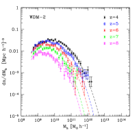
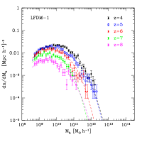
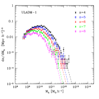
In Table 8, 9 and 10 we quote the values of the coefficients of Eq. (4) best-fitting the halo mass functions from the N-body halo catalogs of WDM, LFDM and ULADM model simulations. For illustrative purposes in Fig. 15 we plot the mass function at from the simulations of WDM-2 (panel a), LFDM-1 (panel b) and ULADM-1 (panel c) models against the best-fitting functions.
| Model | z | ||||
|---|---|---|---|---|---|
| WDM-1 | 4.0 | 0.46688E-01 | -0.15362E-02 | 0.77722E+00 | 0.36452E+12 |
| 5.0 | 0.56763E-01 | -0.15343E-02 | 0.77124E+00 | 0.35490E+12 | |
| 6.0 | 0.68210E-01 | -0.14801E-02 | 0.80043E+00 | 0.35685E+12 | |
| 7.0 | 0.12417E+00 | -0.10537E-02 | 0.88205E+00 | 0.33658E+12 | |
| 8.0 | 0.17072E+00 | -0.87254E-03 | 0.97998E+00 | 0.31569E+12 | |
| WDM-2 | 4.0 | -0.19738E-01 | -0.41804E-02 | 0.86551E+00 | 0.67546E+11 |
| 5.0 | 0.85360E-02 | -0.39280E-02 | 0.80553E+00 | 0.79238E+11 | |
| 6.0 | 0.85360E-02 | -0.39280E-02 | 0.80553E+00 | 0.79238E+11 | |
| 7.0 | 0.11670E-01 | -0.41489E-02 | 0.82052E+00 | 0.80275E+11 | |
| 8.0 | 0.11890E-01 | -0.31869E-02 | 0.86675E+00 | 0.89083E+11 | |
| WDM-3 | 4.0 | -0.29145E-01 | -0.13439E-01 | 0.53411E+00 | 0.25237E+11 |
| 5.0 | 0.21376E-02 | -0.10081E-01 | 0.58836E+00 | 0.27828E+11 | |
| 6.0 | 0.10142E-01 | -0.94886E-02 | 0.59938E+00 | 0.28294E+11 | |
| 7.0 | 0.16513E-01 | -0.97150E-02 | 0.61578E+00 | 0.28749E+11 | |
| 8.0 | 0.17838E-01 | -0.97581E-02 | 0.62047E+00 | 0.28882E+11 | |
| WDM-4 | 4.0 | -0.54437E-01 | -0.12643E-01 | 0.51662E+00 | 0.83804E+10 |
| 5.0 | -0.19856E-01 | -0.15134E-01 | 0.42798E+00 | 0.11073E+11 | |
| 6.0 | 0.44430E-02 | -0.17341E-01 | 0.53405E+00 | 0.87945E+10 | |
| 7.0 | 0.56581E-02 | -0.18033E-01 | 0.55238E+00 | 0.90182E+10 | |
| 8.0 | 0.75246E-02 | -0.18507E-01 | 0.56916E+00 | 0.92176E+10 | |
| WDM-5 | 4.0 | -0.34874E-01 | -0.14503E-01 | 0.30686E+00 | 0.88613E+10 |
| 5.0 | -0.22920E-01 | -0.14582E-01 | 0.29235E+00 | 0.89928E+10 | |
| 6.0 | -0.18762E-01 | -0.19141E-01 | 0.38016E+00 | 0.58888E+10 | |
| 7.0 | 0.40597E-04 | -0.21623E-01 | 0.41057E+00 | 0.58092E+10 | |
| 8.0 | 0.19086E-02 | -0.22924E-01 | 0.43360E+00 | 0.59553E+10 |
| Model | z | ||||
|---|---|---|---|---|---|
| LFDM-1 | 4.0 | 0.77542E-02 | -0.30292E-02 | 0.91358E+00 | 0.98292E+11 |
| 5.0 | 0.14193E+01 | -0.28145E-04 | 0.71418E+00 | 0.16774E+14 | |
| 6.0 | 0.12092E+00 | -0.20581E-02 | 0.91856E+00 | 0.11639E+12 | |
| 7.0 | -0.94165E-01 | -0.38357E-02 | 0.10138E+01 | 0.57870E+11 | |
| 8.0 | 0.28828E+01 | -0.37645E-05 | 0.10240E+01 | 0.59584E+14 | |
| LFDM-2 | 4.0 | -0.29327E-01 | -0.15755E-01 | 0.73613E+00 | 0.19674E+11 |
| 5.0 | 0.97870E-03 | -0.11420E-01 | 0.77712E+00 | 0.21978E+11 | |
| 6.0 | 0.80251E-02 | -0.89361E-02 | 0.79105E+00 | 0.23007E+11 | |
| 7.0 | 0.89883E-02 | -0.90835E-02 | 0.79925E+00 | 0.23181E+11 | |
| 8.0 | 0.18154E-01 | -0.95860E-02 | 0.81578E+00 | 0.23253E+11 | |
| LFDM-3 | 4.0 | -0.32719E-01 | -0.20121E-01 | 0.40862E+00 | 0.68945E+10 |
| 5.0 | -0.13631E-01 | -0.22584E-01 | 0.33976E+00 | 0.78197E+10 | |
| 6.0 | -0.19237E-02 | -0.27440E-01 | 0.23097E+00 | 0.95535E+10 | |
| 7.0 | 0.18435E+00 | -0.57700E-02 | 0.27619E+00 | 0.43788E+11 | |
| 8.0 | 0.19969E+00 | -0.82653E-02 | 0.41080E+00 | 0.23100E+11 |
| Model | z | ||||
|---|---|---|---|---|---|
| ULADM-1 | 4.0 | 0.53670E-01 | -0.80077E-02 | 0.11984E+01 | 0.26093E+11 |
| 5.0 | 0.13686E+00 | -0.60703E-02 | 0.11552E+01 | 0.32254E+11 | |
| 6.0 | 0.30520E+00 | -0.53837E-02 | 0.95829E+00 | 0.61748E+11 | |
| 7.0 | 0.46699E+00 | -0.41026E-02 | 0.10038E+01 | 0.75679E+11 | |
| 8.0 | 0.63537E+00 | -0.24629E-02 | 0.10432E+01 | 0.98482E+11 | |
| ULADM-2 | 4.0 | 0.16547E-01 | -0.37448E-01 | 0.72171E+00 | 0.75500E+10 |
| 5.0 | 0.38302E-01 | -0.43754E-01 | 0.87168E+00 | 0.60405E+10 | |
| 6.0 | 0.72256E-01 | -0.27448E-01 | 0.10546E+01 | 0.59524E+10 | |
| 7.0 | 0.28522E+00 | -0.13903E-01 | 0.69252E+00 | 0.20848E+11 | |
| 8.0 | 0.35025E+00 | -0.11690E-01 | 0.77661E+00 | 0.21250E+11 | |
| ULADM-3 | 4.0 | 0.56134E-02 | -0.93856E-01 | 0.48333E+00 | 0.12463E+10 |
| 5.0 | 0.15222E-01 | -0.18837E+00 | 0.43060E+00 | 0.86619E+09 | |
| 6.0 | 0.14859E-01 | -0.54771E-01 | 0.62784E+00 | 0.11009E+10 | |
| 7.0 | 0.55854E-01 | -0.91105E-01 | 0.36028E+00 | 0.13199E+10 | |
| 8.0 | 0.84951E-01 | -0.88151E-01 | 0.45541E+00 | 0.13210E+10 |
References
- (1) S.L. Finkelstein et al., Astrophys. J. 758, 93 (2012)
- (2) R.J. Bouwens et al., Astrophys. J. 754, 83 (2012)
- (3) P.A. Oesch et al., Astrophys. J. 773, 75 (2013)
- (4) M.A. Schenker et al., Astrophys. J. 768, 196 (2013)
- (5) R.J. McLure et al., Mont. Not. Roy. Astron. Soc. 432, 2696 (2013)
- (6) R.J. Bouwens et al., Astrophys. J. 803, 34 (2015)
- (7) S.L. Finkelstein et al., Astrophys. J. 810, 71 (2015)
- (8) D.J. McLeod et al., Mont. Not. Roy. Astron. Soc. 450, 3032
- (9) R.J. Bouwens et al., in press, arXiv:1506.01035
- (10) J.A. Muoz, A. Loeb, Astrophys. J. 729, 99 (2011)
- (11) J. Jaacks, J.-H. Choi, K. Nagamine, R. Thompson, S. Varghese, Mont. Not. Roy. Astron. Soc. 420, 1606 (2012)
- (12) Z.-Y. Cai et al., Astrophys. J. 785, 65 (2014)
- (13) C.A. Mason, M. Trenti, T. Treu, Astrophys. J. 813, 21 (2015)
- (14) M. Ishigaki et al., Astrophys. J. 799, 12 (2015)
- (15) H. Atek et al., Astrophys. J. 800, 18 (2015)
- (16) H. Atek et al., Astrophys. J. 814, 69 (2015)
- (17) R.C. Livermore, S.L. Finkelstein, J.M. Lotz, arXiv:1604.06799
- (18) D. Coe, L. Bradley, A. Zitrin, Astrophys. J. 800, 84 (2015)
- (19) J.M. Lotz et al., arXiv:1605.06567
- (20) S.V.W. Beckwith et al., Astron. J. 132, 1729 (2006)
- (21) R.S. Ellis et al., Astrophys. J. 763, L7
- (22) G.D. Illingworth et al., Astrophys. J. Supp. 209, 6 (2013)
- (23) R.J. Bouwens et al., arXiv:1608.00966
- (24) R.J. Bouwens et al., arXiv:1610.00283
- (25) P. J. E. Peebles, Principles of Physical Cosmology, Princeton University Press (1993)
- (26) D. N. Spergel et al., Astrophys. J. Suppl. Ser. 148, 175 (2003)
- (27) M. Tegmark et al., Phys. Rev. D. 69, 103501 (2004)
- (28) R. Massey et al., Nature (London) 445, 286 (2007)
- (29) Planck Collaboration: P.A.R. Ade et al., Astron. & Astrophys. in press, arXiv:1502.01589
- (30) G. Jungman, M. Kamionkowski, K. Griest, Phys. Rep. 267, 195 (1996)
- (31) G. Bertone, D. Hooper, J. Silk, Phys. Rep. 405, 279 (2005)
- (32) D.J.E. Marsh, Phys. Rep. 643, 1 (2016)
- (33) S.J. Asztalos et al., Phys. Rev. Lett. 104, 041301 (2010)
- (34) K.A. Olive et al., Chin. Phys. 38, 090001 (2014)
- (35) W. Liao, X.-H. Wu, H. Zhou, Phys. Rev. D 89, 093017 (2014)
- (36) S. Mertens et al., JCAP 1502, 020 (2015)
- (37) M.D. Campos, W. Rodejohann, arXiv:1605.02918
- (38) S. Dodelson, L.M. Widrow, Phys. Rev. Lett. 72, 17 (1994); G.M. Fuller, A. Kusenko, I. Mocioiu, S. Pascoli, Phys. Rev. D 68, 103002 (2003); K. Abazajian, Phys. Rev. D 73, 063513 (2006); D. Boyanovsky, H.J. de Vega, N.G. Sanchez, Phys. Rev. D 78, 063546 (2008); H.J. de Vega, P. Salucci, N.G. Sanchez, New Astron. 17, 653 (2012)
- (39) A. V. Maccio et al., Mont. Not. R. Astron. Soc. 424,1105 (2012); M. R. Lovell et al., Mont. Not. R. Astron. Soc. 420, 2318 (2012)
- (40) P. Svrcek, E. Witten, JHEP 06, 051 (2006)
- (41) A. Arvanitaki et al., Phys. Rev. D 81, 123530 (2010)
- (42) J.E. Kim, D.J.E. Marsh, Phys. Rev. D 93, 025027 (2016)
- (43) M. Khlopov, B.A. Malomed, I.B. Zeldovich, Mont. Not. Roy. Astron. Soc. 215, 575 (1985)
- (44) W.H. Press, B.S. Ryden, D.N. Spergel, Phys. Rev. Lett. 64, 1084 (1990)
- (45) S.-J. Sin, Phys. Rev. D 50, 3650 (1994)
- (46) J.-W. Lee, I.-G. Koh, Phys. Rev. D 53, 2236 (1996)
- (47) W. Hu, R. Barkana, A. Gruzinov, Phys. Rev. Lett. 85, 1158 (2000)
- (48) D.J.E. Marsh, P.G. Ferreira, Phys. Rev. D 82, 103528 (2010)
- (49) D.J.E. Marsh, J. Silk, Mont. Not. Roy. Astron. Soc. 437, 2652 (2014)
- (50) H.-Y. Schive, T. Chiueh, T. Broadhurst, Nat. Phys. 10, 496 (2014)
- (51) L. Hui, J.P. Ostriker, S. Tremaine, E. Witten, arXiv:1610.08297
- (52) B. Moore, Nature (London) 370, 629 (1994)
- (53) R. Kuzio de Naray, T. Kaufmann, Mon. Not. R. Astron. Soc. 414, 3617 (2011)
- (54) A. Klypin, A. V. Kravtsov, O. Valenzuela, F. Prada, Astrophys. J. 522, 82 (1999)
- (55) B. Moore et al., Astrophys. J. 524, L19 (1999)
- (56) M. Boylan-Kolchin, J. S. Bullock, M. Kaplinghat, Mon. Not. R. Astron. Soc. 415, L40 (2011)
- (57) M. Boylan-Kolchin, J. S. Bullock, M. Kaplinghat, Mon. Not. R. Astron. Soc. 422, 1203 (2012)
- (58) N. I. Libeskind et al., Mon. Not. R. Astron. Soc. 374, 16 (2007)
- (59) A. V. Macciò et al., Mon. Not. R. Astron. Soc. 402, 1995 (2010)
- (60) A. Pontzen, F. Governato, Mon. Not. R. Astron. Soc. 421, 3464 (2012)
- (61) J. Paarrubia, A. Pontzen, M. G. Walker, S. E. Koposov, Astrophys. J. 759, L42 (2012)
- (62) S. Garrison-Kimmel, M. Rocha, M. Boylan-Kolchin, J. S. Bullock, J. Lally , Mon. Not. R. Astron. Soc. 433, 3539 (2013)
- (63) D.N. Spergel, P.J. Steinhardt, Phys. Rev. Lett. 84, 3760 (2000)
- (64) M. Kaplinghat, S. Tulin, H.-B. Yu, Phys. Rev. D 89, 5009 (2014)
- (65) F.-Y. Cyr-Racine et al., Phys. Rev. D 93, 123527 (2016)
- (66) W. Hu, Astrophys. J. 506, 485 (1998)
- (67) M. Kunz, S. Nesseris, I. Sawicki, Phys. Rev. D 94, 023510 (2016)
- (68) M. Kopp, C. Skordis, D.B. Thomas, Phys. Rev. D 94, 043512 (2016)
- (69) J. Jaacks, R. Thompson, K. Nagamine, Astrophys. J. 766, 94 (2013)
- (70) B.W. O’Shea, J.H. Wise, H. Xu, M.L. Norman, Astrophys. J. 807, L12 (2015)
- (71) R. Hlozek, D.J.E. Marsh, D. Grin, R. Allison, J. Dunkley, E. Calabrese, arXiv:1607.08208; R. Hlozek, D. Grin, D. J.E. Marsh, P.G. Ferreira, Phys. Rev. D 91, 103512 (2015)
- (72) S. Das, N. Weiner, Phys. Rev. D 84, 123511 (2011)
- (73) S. Agarwal, P.-S. Corasaniti, Phys. Rev. D 91, 123509 (2015)
- (74) M. Viel, G.D. Becker, J.S. Bolton, M.G. Haehnelt, Phys. Rev. D 88, 043502 (2013)
- (75) J. Baur, N. Palanque-Delabrouille, C. Yeche, C. Magneville, M. Viel, JCAP 1608, 012 (2016)
- (76) A. Garzilli, A. Boyarsky, O. Ruchayskiy, arXiv:1510.07006
- (77) F. Pacucci, A. Mesinger, and Z. Haiman, Mont. Not. Roy. Astron. Soc., 435, L53 (2013)
- (78) A. Lapi, L. Danese, JCAP 1509, 003 (2015)
- (79) N. Menci, A. Grazian, M. Castellano, N.G. Sanchez, Astrophys. J. 825, L1 (2016)
- (80) C. Schultz, J. Orobe, K. Abazajian, and J.S. Bullock, Mont. Not. Roy. Astron. Soc. 442, 1597 (2014)
- (81) B. Bozek, D.J.E. Marsh, J. Silk, and R.F.G. Wyse, Mont. Not. Roy. Astron. Soc., 450, 209 (2015)
- (82) H.-Y. Schive, T. Chiueh, T. Broadhurst, K.W. Huang, Astrophys. J. 818, 89 (2016)
- (83) G.R. Meurer, T.M. Heckman, D. Calzetti, Astrophys. J. 521, 64 (1999)
- (84) R. Smit et al., Astrophys. J. 756, 14 (2012)
- (85) N. Mashian, P.A. Oesch, A. Loeb, Mont. Not. Roy. Astron. 455, 2101 (2016)
- (86) C.J. Willott et al, Astron. J. 145, 4 (2013)
- (87) M. Ouchi et al., Astrophys. J. 706, 1136 (2009)
- (88) R.A.A. Bowler et al., Mont. Not. Roy. Astron. Soc. 440, 2810 (2014)
- (89) R.A.A. Bowler et al., Mont. Not. Roy. Astron. Soc. 452, 1817 (2015)
- (90) R.A.A. Bowler, J.S. Dunlop, R.J. McLure, D.J. McLeod, Mont. Not. Roy. Astron. Soc. 466, 3612 (2017)
- (91) R.C. Kennicutt, Ann. Rev. Astron. & Astrophys. 36, 189 (1998)
- (92) A. Lewis, A. Challinor, A. Lasenby, Astrophys. J. 538 473 (2000)
- (93) P. Bode, J. P. Ostriker, N. Turok, Astrophys. J. 556 93 (2001)
- (94) R. Teyssier, Astron. & Astrophys. 385, 337 (2002)
- (95) S. Prunet et al., Astrophys. J. Supp. 178, 179 (2008)
- (96) M. Davis, G. Efstathiou, C. S. Frenk, S. D. M. White, Astrophys. J. 292, 371 (1985)
- (97) F. Roy, V. Bouillot, Y. Rasera, Astron. & Astrophys. 564, A13 (2014)
- (98) J. S. Bullock et al., Astrophys. J. 555, 240 (2001)
- (99) J. Courtin et al., Mont. Not. Roy. Astron. Soc. 410, 1911 (2011)
- (100) M. Götz, J, Sommer-Larsen, Ap&SS 281, 415 (2002)
- (101) M. Götz, J, Sommer-Larsen, Ap&SS 284, 341 (2003)
- (102) J. Wang, S. D. M. White, Mont. Not. Roy. Astron. Soc. 380, 93 (2007)
- (103) M. R. Lovell et al., Mont. Not. Roy. Astron. Soc. 439, 300 (2014)
- (104) H.-Y. Schive et al., Phys. Rev. Lett. 113, 261302 (2014)
- (105) R.K. Sheth, G. Tormen, Mont. Not. Roy. Astron. Soc. 308, 119 (1999)
- (106) T. Kitayama, Y. Suto, Mont. Not. Roy. Astron. Soc. 280, 638 (1996)
- (107) R. E. Angulo, O. Hahn, T. Abel, Mont. Not. Roy. Astron. Soc. 434, 3337 (2013)
- (108) P. Colin, O. Valenzuela, V. Avila-Reese, Astrophys. J. 673, 203 (2008)
- (109) S. Tremaine, J.E. Gunn, Phys. Rev. Lett. 42, 407 (1979)
- (110) B. Schwabe, J.C. Niemeyer, J.F. Engels, arXiv:1606.05151
- (111) J. Veltmaat, J.C. Niemeyer, arXiv:1608.00802
- (112) M. Trenti, R. Perna, R. Jimenez, Astrophys. J. 802, 103 (2015)
- (113) R.J. Bouwens et al., Astrophys. J. 793, 115 (2014)
- (114) A. Cooray, M. Milosavljevic, Astrophys. J. 627, L89
- (115) A. Gelman, D.B. Rubin, Stat. Sci., 7, 457 (1992)
- (116) J.H. Wise et al., Mont. Not. Roy. Astron. Soc. 442, 2560 (2014)
- (117) C. Liu et al., Mont. Not. Roy. Astron. Soc. 462, 235 (2016)
- (118) P. Dayal, A. Mesinger, F. Pacucci, Astrophys. J. 806, 67 (2015)
- (119) X. Kang, A.V. Macciò, A.A. Dutton, Astrophys. J. 767, 22 (2013)
- (120) N. Menci et al., Astrophys. J. 836, 61 (2017)
- (121) Planck Collaboration: N. Aghanim et al., arXiv:1605.02985
- (122) D. Munshi et al., Mont. Not. Roy. Astron. Soc. 442, 3427 (2014), arXiv:1403.1531
- (123) E. Calabrese et al., arXiv:1406.4794; K. Smith, S. Ferraro, arXiv:1607.01769