Renormalized stress-energy tensor for stationary black holes

Abstract

We continue the presentation of the pragmatic mode-sum regularization (PMR) method for computing the renormalized stress-energy tensor (RSET). We show in detail how to employ the $t$-splitting variant of the method, which was first presented for $\left\langle\phi^{2}\right\rangle_{ren}$, to compute the RSET in a stationary, asymptotically-flat background. This variant of the PMR method was recently used to compute the RSET for an evaporating spinning black hole. As an example for regularization, we demonstrate here the computation of the RSET for a minimally-coupled, massless scalar field on Schwarzschild background in all three vacuum states. We discuss future work and possible improvements of the regularization schemes in the PMR method.

I Introduction

Computation of the renormalized stress-energy tensor (RSET) $\left\langle T_{\alpha\beta}\right\rangle_{ren}$ is important for studying the effects of a quantum field on the metric. For example, the field can be a minimally-coupled, massless scalar field $\phi\left(x\right)$ satisfying the d’Alembertian equation

$$\square\phi=0.$$ (1)

The back-reaction on the metric is described by the semiclassical Einstein equation

$$G_{\alpha\beta}=8\pi\left\langle T_{\alpha\beta}\right\rangle_{ren},$$ (2)

where $G_{\alpha\beta}$ is the Einstein tensor. The most notable physical phenomenon described by Eqs. (1)-(2) is evaporation of a black hole (BH) due to Hawking radiation Hawking - Particle creation by black holes .

The naive computation of the stress-energy tensor yields a divergent mode-sum. In flat spacetime one can use the normal ordering operator to regularize this divergence. Unfortunately, normal ordering is not defined in curved spacetime. In 1965 DeWitt Dewitt - Dynamical theory of groups and fields used the point-splitting method (first introduced by Schwinger Schwinger ) to renormalize $\left\langle\phi^{2}\right\rangle$, and in 1976 Christensen Christensen 1976 adapted it for the computation of the RSET. In the point-splitting method one can compute the renormalized value of a quantity which is quadratic in the field (or its derivatives) at a point $x$, e.g. $\left\langle\phi^{2}\left(x\right)\right\rangle$, by splitting the point $x$ into two points $x,x^{\prime}$, and considering a two-point function (TPF) of the form $\left\langle\phi\left(x\right)\phi\left(x^{\prime}\right)\right\rangle$. Then one subtracts from the TPF a known counter term and takes the limit $x^{\prime}\to x$.

Although the recipe for computing the RSET is known for four decades it is still a great challenge to compute it generically, even for a prescribed background. The difficulty is caused by the limit $x^{\prime}\to x$. This limit can be taken rather simply if the modes are known analytically, however, in most cases, and in particular for BHs backgrounds, the modes are known only numerically, which turns the limit into a very difficult task.

To overcome this difficulty, Candelas, Howard, Anderson and others Candelas - 1979 - phi2 Schwarzschild ; Candelas =000026 Howard - 1984 - phi2 Schwrazschild ; Howard - 1984 - Tab Schwarzschild ; Anderson - 1990 - phi2 static spherically symmetric ; Anderson - 1995 - Tab static spherically symmetric developed a method to implement point-splitting numerically. This method relied on a forth order WKB, which is very hard to compute in a Lorentzian background, so they have used Wick’s rotation and computed the RSET in the Euclidean sector. More recently, Taylor and Breen introduced Peter taylor a more sophisticated version of the traditional method, which does not require a WKB approximation, but is still using the Euclidean sector.

Unfortunately, the Euclidean sector does not exist for most backgrounds, and so the aforementioned methods were developed for static, spherically-symmetric backgrounds. This leaves out all possible dynamical backgrounds, which are of great interest, as well as backgrounds of spinning BHs, such as Kerr, which are stationary but not static.

Recently, Levi and Ori introduced Levi =000026 Ori - 2015 - t splitting regularization ; Levi =000026 Ori - 2016 - theta splitting regularization ; Levi =000026 Ori - 2016 - RSET the pragmatic mode-sum regularization (PMR) method. This method does not rely on the Euclidean sector, and all computations are done directly in the Lorentzian background. The PMR method requires the background to admit a single symmetry (a Killing field), and takes different variants depending on the symmetry exploited.

So far, two variants of PMR were introduced in detail for the computation of $\left\langle\phi^{2}\right\rangle_{ren}$: the $t$-splitting variant Levi =000026 Ori - 2015 - t splitting regularization , for stationary backgrounds, and the Angular-splitting variant Levi =000026 Ori - 2016 - theta splitting regularization , for spherically-symmetric backgrounds. A third variant, the $\varphi$-splitting (also named the azimuthal-splitting), for axially-symmetric backgrounds was introduced briefly Levi =000026 Ori - 2016 - RSET .

Although the details of implementing the method to compute the RSET were not given yet, results for the RSET obtained using the PMR method were already presented: The RSET in Schwarzschild in the Unruh state was displayed using all three variants Levi =000026 Ori - 2016 - RSET . In a more recent work, the $t$-splitting and $\varphi$-splitting variants were used to compute the RSET in Kerr in the Unruh state Levi Eilon Ori and DeMeent - 2016 - Kerr .

In this paper we fill in the gaps for the $t$-splitting variant by showing in detail how to utilize it to compute the RSET for an asymptotically-flat, stationary background. For briefness we restrict our attention to a minimally-coupled, massless scalar field. We then harness it to compute the RSET in Schwarzschild in all three vacuum states.

Further details of how to implement PMR for the RSET in the angular-splitting variant for spherically symmetric backgrounds, and in the $\varphi$-splitting variant for axially-symmetric backgrounds will be given elsewhere Preparation .

This paper is organized as follows: Section II presents the basic point-splitting scheme for the RSET. Section III presents the the implementation of $t$-splitting for the calculation of the RSET and section IV presents the detailed computation of the RSET in Schwarzschild. In section V we discuss the PMR method in general as well as future research.

II The point-splitting scheme

The computation of the RSET in the point-splitting scheme, as formulated by Christensen Christensen 1976 , takes the form

$$\left\langle T_{\mu\nu}\left(x\right)\right\rangle_{ren}=\lim_{x^{\prime}\to x}\left[\left\langle T_{\mu\nu}\left(x,x^{\prime}\right)\right\rangle-C_{\mu\nu}\left(x,x^{\prime}\right)\right],$$ (3)

where we use $C_{\mu\nu}\left(x,x^{\prime}\right)$ for Christensen’s counter-term tensor, which depends on the bi-scalar $\sigma\left(x,x^{\prime}\right)$, its covariant derivatives and on the metric. The bi-scalar $\sigma\left(x,x^{\prime}\right)$ is defined to be half the geodesic distance squared, of the short geodesic connecting $x$ and $x^{\prime}$. The explicit expression for $C_{\mu\nu}\left(x,x^{\prime}\right)$ is very long and can be found in Ref. Christensen 1976 . The quantity $\left\langle T_{\mu\nu}\left(x,x^{\prime}\right)\right\rangle$, which we will name the two-point stress tensor (TPST) is analogous to the TPF used in the regularization of $\left\langle\phi^{2}\right\rangle$. If we denote the symmetric TPF (also known as the Hadamard function) by

$$G^{\left(1\right)}\equiv\left\langle\phi\left(x\right)\phi\left(x^{\prime}\right)\right\rangle+\left\langle\phi\left(x^{\prime}\right)\phi\left(x\right)\right\rangle=\left\langle\left[\phi\left(x\right)\phi\left(x^{\prime}\right)\right]_{+}\right\rangle,$$ (4)

where $\left[\right]_{+}$ denotes anti-commutation, then the TPST explicit form for a minimally-coupled, massless scalar field is

$$\left\langle T_{\mu\nu}\left(x,x^{\prime}\right)\right\rangle=\frac{1}{4}\left(\bar{g}_{\mu}^{\beta^{\prime}}G_{;\beta^{\prime}\nu}^{\left(1\right)}+\bar{g}_{\nu}^{\beta^{\prime}}G_{;\mu\beta^{\prime}}^{\left(1\right)}\right)-\frac{1}{4}g_{\mu\nu}\bar{g}_{\sigma}^{\beta^{\prime}}G_{;\beta^{\prime}}^{\left(1\right);\sigma}.$$ (5)

Primed derivatives are taken at $x^{\prime}$, e.g.

$$G_{;\beta^{\prime}\nu}^{\left(1\right)}=\left\langle\left[\phi_{;\nu}\left(x\right)\phi_{;\beta^{\prime}}\left(x^{\prime}\right)\right]_{+}\right\rangle,$$

and $\bar{g}_{\mu}^{\beta^{\prime}}$ is the bi-vector of parallel transport, which transfers a vector at $x^{\prime}$ to $x$, satisfying

$$\sigma_{;\mu}=-\bar{g}_{\mu}^{\beta^{\prime}}\sigma_{;\beta^{\prime}}.$$ (6)

For a concrete split it is straightforward to compute $\bar{g}_{\mu}^{\beta^{\prime}}$ as a series in the separation, by solving the parallel transport equation order by order. For further details on the bi-scalar $\sigma$, and bi-vector of parallel transport $\bar{g}_{\mu}^{\beta^{\prime}}$ we refer to Christensen 1976 .

We now take the recipe by Christensen and rewrite it to obtain a form which is more natural for concrete computations. Notice that the RHS of Eq. (5) has the form of a trace-reversed tensor. It is convenient to use this structure to reverse the trace of the equation. Denoting with a tilde a trace reversed tensor, Eq. (5) takes the form

$$\left\langle\tilde{T}_{\mu\nu}\left(x,x^{\prime}\right)\right\rangle=\frac{1}{4}\left(\bar{g}_{\mu}^{\beta^{\prime}}G_{;\beta^{\prime}\nu}^{\left(1\right)}+\bar{g}_{\nu}^{\beta^{\prime}}G_{;\mu\beta^{\prime}}^{\left(1\right)}\right).$$

Substituting the Hadamard function

$$\left\langle\tilde{T}_{\mu\nu}\left(x,x^{\prime}\right)\right\rangle=\frac{1}{4}\left(\delta_{\mu}^{\alpha}\bar{g}_{\nu}^{\beta^{\prime}}+\delta_{\nu}^{\alpha}\bar{g}_{\mu}^{\beta^{\prime}}\right)\left\langle\left[\phi_{,\alpha}\left(x\right)\phi_{,\beta^{\prime}}\left(x^{\prime}\right)\right]_{+}\right\rangle.$$

Inserting it to the trace reversed version of Eq. (3) one obtains

$$\left\langle\tilde{T}{}_{\mu\nu}\left(x\right)\right\rangle_{ren}=\lim_{x^{\prime}\to x}\left[\frac{1}{4}\left(\delta_{\mu}^{\alpha}\bar{g}_{\nu}^{\beta^{\prime}}+\delta_{\nu}^{\alpha}\bar{g}_{\mu}^{\beta^{\prime}}\right)\left\langle\left[\phi_{,\alpha}\left(x\right)\phi_{,\beta^{\prime}}\left(x^{\prime}\right)\right]_{+}\right\rangle-\tilde{C}_{\mu\nu}\left(x,x^{\prime}\right)\right],$$

which can also be written in the form

$$\left\langle\tilde{T}{}_{\mu\nu}\left(x\right)\right\rangle_{ren}=\lim_{x^{\prime}\to x}\left(\delta_{\mu}^{\alpha}\bar{g}_{\nu}^{\beta^{\prime}}+\delta_{\nu}^{\alpha}\bar{g}_{\mu}^{\beta^{\prime}}\right)\left[\frac{1}{4}\left\langle\left[\phi_{,\alpha}\left(x\right)\phi_{,\beta^{\prime}}\left(x^{\prime}\right)\right]_{+}\right\rangle-\frac{1}{2}\delta_{\alpha}^{\sigma}\left(\bar{g}^{-1}\right)_{\beta^{\prime}}^{\rho}\tilde{C}_{\sigma\rho}\left(x,x^{\prime}\right)\right].$$

The limit of the parentheses is finite, as well as the limit of the brackets. So we can take the limit of the parentheses, which is trivial, since the limit of the bi-vector $\bar{g}_{\mu}^{\beta^{\prime}}$ is the unit matrix $\delta_{\mu}^{\beta^{\prime}}$ (Ref. Christensen 1976 ). Bringing the parentheses back into the brackets yields

$$\left\langle\tilde{T}{}_{\mu\nu}\left(x\right)\right\rangle_{ren}=\lim_{x^{\prime}\to x}\left|\frac{1}{4}\left\langle\left[\phi_{,\mu}\left(x\right)\phi_{,\nu}\left(x^{\prime}\right)\right]_{+}\right\rangle+\frac{1}{4}\left\langle\left[\phi_{,\nu}\left(x\right)\phi_{,\mu}\left(x^{\prime}\right)\right]_{+}\right\rangle\right.\\ \left.-\frac{1}{2}\left(\left(\bar{g}^{-1}\right)_{\nu}^{\rho}\tilde{C}_{\mu\rho}\left(x,x^{\prime}\right)+\left(\bar{g}^{-1}\right)_{\mu}^{\rho}\tilde{C}_{\nu\rho}\left(x,x^{\prime}\right)\right)\right].$$

Note that here we deviated from the usual covariant bi-tensor notation, which is constructed to allow two different coordinate systems at $x$ and $x^{\prime}$. We use a single coordinate system, and take derivative according to the coordinate system of point $x$ on the field at point $x^{\prime}$. This approach is less systematic, but proves to be very useful for computations.

For convenience we define a new quantity, which is a symmetrized version of the Christensen tensor $\tilde{C}_{\sigma\rho}\left(x,x^{\prime}\right)$ multiplied by the bi-vector $\left(\bar{g}^{-1}\right)_{\mu}^{\rho}$. Henceforth we will call this quantity the counter-term

$$\tilde{L}_{\mu\nu}\left(x,x^{\prime}\right)\equiv\frac{1}{2}\left(\left(\bar{g}^{-1}\right)_{\nu}^{\rho}\tilde{C}_{\mu\rho}\left(x,x^{\prime}\right)+\left(\bar{g}^{-1}\right)_{\mu}^{\rho}\tilde{C}_{\nu\rho}\left(x,x^{\prime}\right)\right),$$ (7)

and we conclude that

$$\left\langle\tilde{T}{}_{\mu\nu}\left(x\right)\right\rangle_{ren}=\lim_{x^{\prime}\to x}\left[\frac{1}{4}\left\langle\left[\phi_{,\mu}\left(x\right)\phi_{,\nu}\left(x^{\prime}\right)\right]_{+}\right\rangle+\frac{1}{4}\left\langle\left[\phi_{,\nu}\left(x\right)\phi_{,\mu}\left(x^{\prime}\right)\right]_{+}\right\rangle-\tilde{L}_{\mu\nu}\left(x,x^{\prime}\right)\right].$$ (8)

One example that illustrates how $\tilde{L}_{\mu\nu}$ captures better the essence of the singularity is the trace of the RSET for a minimally-coupled, massless scalar field in a Ricci-flat solution. The trace of Christensen’s tensor $C_{\sigma}^{\,\,\sigma}\left(x,x^{\prime}\right)$ in such a case has no singular piece. Nevertheless, if one tries to naively (i.e. with no split) compute the trace of the stress tensor one finds it diverges. The trace $L_{\sigma}^{\,\,\sigma}\left(x,x^{\prime}\right)$ however, has a singular term proportional to $1/\sigma\left(x,x^{\prime}\right)$, which corresponds directly to the divergence of the mode-sum.

III Regularization of the stress tensor

Continuing the line taken in Levi =000026 Ori - 2015 - t splitting regularization we would like to build a scheme that will enable the computation of the RSET using the mode-sum at the coincidence, based on the analytic point-splitting recipe given by Christensen. We claim it is possible given that the space-time admits some symmetry (a Killing field), and for each symmetry the scheme takes a different form. Here we present the $t$-splitting variant which is applicable for asymptotically-flat, stationary backgrounds. We use the coordinates $t,\,r,\,\theta,\,\varphi$, and the metric $g_{\alpha\beta}$ depends on $r,\,\theta,\,\varphi$ but not on $t$. In the limit $r\to\infty$ the metric takes the form

$$ds^{2}=-dt^{2}+dr^{2}+r^{2}d\Omega^{2},$$

where $d\Omega^{2}\equiv d\theta^{2}+\sin^{2}\theta d\varphi^{2}$.

We shall first address the case of a background with a regular center, and in Sec. III.2 we will show the simple adjustments for the case of an eternal BH. In a stationary background one can decompose the modes in the form

$$\phi\left(x\right)=\int_{0}^{\infty}d\omega\sum_{l=0}^{\infty}\sum_{m=-l}^{l}\left(f_{\omega lm}\left(x\right)a_{\omega lm}+f_{\omega lm}^{*}\left(x\right)a_{\omega lm}^{\dagger}\right)$$ (9)

$$f_{\omega lm}\left(x\right)=e^{-i\omega t}Y_{lm}\left(\theta,\varphi\right)\bar{\psi}_{\omega lm}\left(r,\theta,\varphi\right),$$ (10)

where $a_{\omega lm}^{\dagger},\,a_{\omega lm}$ are the creation and annihilation operators and $Y_{lm}\left(\theta,\varphi\right)$ are the spherical harmonics functions. In a non-eternal, asymptotically-flat background one can choose the initial conditions for the modes $f_{\omega lm}$ at past null infinity to be the same as in flat space, which defines a vacuum state $\left|0\right\rangle$ such that $a_{\omega lm}\left|0\right\rangle=0$ for all $\omega lm$. The modes evolve according to the d’Alembertian equation

$$\square f_{\omega lm}=0,$$

which yields a differential equation for $\bar{\psi}_{\omega lm}\left(r,\theta,\varphi\right)$ that can in general be solved numerically. It is important to note that, unless specifically stated otherwise, all the integrals over $\omega$ in this paper are generalized integrals, as defined in Appendix A.

It is very helpful to first examine the naive divergent calculation one gets when trying to calculate the stress-tensor without splitting the points

$$\left\langle\tilde{T}{}_{\mu\nu}\left(x\right)\right\rangle_{naive}=\frac{1}{2}\left\langle\left[\phi_{,\mu}\left(x\right)\phi_{,\nu}\left(x\right)\right]_{+}\right\rangle=\hbar\int_{0}^{\infty}d\omega\sum_{l=0}^{\infty}\sum_{m=-l}^{l}\Re\left\{f_{\omega lm,\mu}\left(x\right)f_{\omega lm,\nu}^{*}\left(x\right)\right\},$$ (11)

where $\Re$ denoted the real part of a complex number. The sum over $m$ is a finite sum, and due to asymptotic flatness the sum over $l$ converges . So one can define

$$F_{\mu\nu}\left(\omega,x\right)\equiv\sum_{l=0}^{\infty}\sum_{m=-l}^{l}\Re\left\{f_{\omega lm,\mu}\left(x\right)f_{\omega lm,\nu}^{*}\left(x\right)\right\},$$ (12)

where the tensor $F_{\mu\nu}$ can be computed numerically. Inserting it back to Eq. (11) we get

$$\left\langle\tilde{T}{}_{\mu\nu}\left(x\right)\right\rangle_{naive}=\hbar\int_{0}^{\infty}F_{\mu\nu}\left(\omega,x\right)d\omega,$$

which is of course divergent for most of the non-vanishing components, e.g. to leading order $F_{tt}\left(\omega,x\right)\propto\omega^{3}$.

Returning to the regularization scheme in Eq. (8), we choose to split the points in the direction of the symmetry. For the stationary backgrounds considered in this paper we split in the $t$ direction, so the points are

$$x=(t,r,\theta,\varphi),\,x^{\prime}=(t+\varepsilon,r,\theta,\varphi),$$

and taking the limit $x^{\prime}\to x$ corresponds to taking $\varepsilon\to 0$. For this type of split the modes satisfy

$$f_{\omega lm}\left(x^{\prime}\right)=f_{\omega lm}\left(x\right)e^{-i\omega\varepsilon}.$$

Using this identity together with the definition of $F_{\mu\nu}\left(\omega,x\right)$ in Eq. (12) one can recast Eq. (8) to get

$$\left\langle\tilde{T}{}_{\mu\nu}\left(x\right)\right\rangle_{ren}=\lim_{\varepsilon\to 0}\left[\hbar\int_{0}^{\infty}F_{\mu\nu}\left(\omega,x\right)\cos\left(\omega\varepsilon\right)d\omega-\tilde{L}_{\mu\nu}\left(x,\varepsilon\right)\right],$$ (13)

where the counter-term is now considered as a function of the point $x$ and $\varepsilon$. If we expand it in $\varepsilon$ it takes the general form

$$\frac{1}{\hbar}\tilde{L}_{\mu\nu}\left(\varepsilon\right)=a_{\mu\nu}\left(x\right)\varepsilon^{-4}+b_{\mu\nu}\left(x\right)\varepsilon^{-2}+c_{\mu\nu}\left(x\right)\varepsilon^{-1}+d_{\mu\nu}\left(x\right)\ln\left(\mu\varepsilon\right)+e_{\mu\nu}\left(x\right)+O\left(\varepsilon\right),$$ (14)

where $a_{\mu\nu}\left(x\right),b_{\mu\nu}\left(x\right),c_{\mu\nu}\left(x\right),d_{\mu\nu}\left(x\right),e_{\mu\nu}\left(x\right)$ are local tensors that depend on the metric, and $\mu$ is the unknown parameter that corresponds to the scale-ambiguity in the regularization (see Ref. Christensen 1976 ).

One can now decompose $\tilde{L}_{\mu\nu}\left(\varepsilon\right)$ to its Fourier components, using the following identities ($\gamma$ is Euler’s constant) :

$$\int_{0}^{\infty}\omega^{3}\cos\left(\omega\varepsilon\right)d\omega =6\varepsilon^{-4}$$

$$\int_{0}^{\infty}\omega\cos\left(\omega\varepsilon\right)d\omega =-\varepsilon^{-2}$$

$$\int_{0}^{\infty}\ln\left(\omega\right)\cos\left(\omega\varepsilon\right)d\omega =-\frac{\pi}{2}\varepsilon^{-1}$$

$$\int_{0}^{\infty}\frac{1}{\omega+\mu e^{-\gamma}}\cos\left(\omega\varepsilon\right)d\omega =-\ln\left(\mu\varepsilon\right)+O\left(\varepsilon\right).$$

Inserting it back to Eq. (13) one obtains

$$\left\langle\tilde{T}{}_{\mu\nu}\left(x\right)\right\rangle_{ren}=\hbar\lim_{\varepsilon\to 0}\left[\int_{0}^{\infty}F_{\mu\nu}^{Reg}\left(\omega,x\right)\cos\left(\omega\varepsilon\right)d\omega\right]-\hbar e_{\mu\nu}\left(r\right),$$ (15)

where

$$F_{\mu\nu}^{Reg}\left(\omega,x\right)\equiv F_{\mu\nu}\left(\omega,x\right)-F_{\mu\nu}^{Sing}\left(\omega,x\right)$$ (16)

and

$$F_{\mu\nu}^{Sing}\left(\omega,x\right)\equiv\frac{1}{6}a_{\mu\nu}\omega^{3}-b_{\mu\nu}\omega-\frac{2}{\pi}c_{\mu\nu}\ln\left(\omega\right)-d_{\mu\nu}\frac{1}{\omega+\mu e^{-\gamma}}.$$ (17)

Interchanging the limit and integral in Eq. (15) we obtain

$$\left\langle\tilde{T}{}_{\mu\nu}\left(x\right)\right\rangle_{ren}=\hbar\int_{0}^{\infty}F_{\mu\nu}^{Reg}\left(\omega,x\right)d\omega-\hbar e_{\mu\nu}.$$ (18)

This interchanging is not trivial, and we address it in the next subsection.

We emphasis that the integral over $\omega$ in Eq. (18) is a generalized integral, and converges as such. Namely, it might contain oscillation at large $\omega$. To pragmatically compute the generalized integral we use the method of self-cancellation which is described in App. A. Once $\left\langle\tilde{T}{}_{\mu\nu}\left(x\right)\right\rangle_{ren}$ is computed one can trace-reverse it to obtain $\left\langle T_{\mu\nu}\left(x\right)\right\rangle_{ren}$.

III.1 Blind spots

The idea behind the interchanging of the limit with the integral in Eq. (15) is that the decomposition of the counter-term would contain all the information about the divergent part of $F_{\mu\nu}\left(\omega,x\right)$, and so one can simply set $\varepsilon$ to zero in the integral. Unfortunately it is not necessarily true. One can imagine a function $B\left(\omega\right)$, for which the integral

$$\int_{0}^{\infty}B\left(\omega\right)\cos\left(\omega\varepsilon\right)d\omega$$

is identically zero, for any $\varepsilon\neq 0$. Yet at the coincidence, namely $\varepsilon=0$, the integral diverges. These types of functions we name blind spots . It is quite simple to find not just one, but a family of blind spots

$$B_{n}\left(\omega\right)=\omega^{2n},\,\,\,n\in 0,1,2,3...$$

With this concept in mind, we return to Eq. (15) and see that there might be a singular part in $F_{\mu\nu}\left(\omega,x\right)$ that one can not learn about from the counter-term. So the integral over $F_{\mu\nu}^{Reg}\left(\omega,x\right)$ does not necessarily have to converge, as $F_{\mu\nu}^{Reg}\left(\omega,x\right)$ might contain blind spots. This is quite manageable, as one can classify the problematic blind spot and simply remove it by using techniques similar to self cancellation, discussed in App. A.

If we assume that the only blind spots are of the form $B_{n}\left(\omega\right)$ (although we do not prove it), then we expect only $\omega^{2}$ or $\omega^{0}$ to appear, as we expect the most singular part in $F_{\mu\nu}\left(\omega,x\right)$ to correspond to the most singular term in the counter-term, which is proportional to $\omega^{3}$. In reality, we did not come across any blind spot in the $t$-splitting, so our best guess is that this blind spots do not exist in $F_{\mu\nu}\left(\omega,x\right)$.

Note that the family of blind spots we presented here was not a blind spot in the calculation for $\left\langle\phi^{2}\right\rangle_{ren}$ in Levi =000026 Ori - 2015 - t splitting regularization . This is due to the fact that the counter-term used there was developed to an arbitrary split, and in the case of the RSET the Christensen tensor was calculated for a symmetric split only. One can also see it by noticing that for $\left\langle\phi^{2}\right\rangle_{ren}$ the decomposition was carried out using $e^{i\omega\varepsilon}$ and here it is done using $\cos\left(\omega\varepsilon\right)$. Taking $\omega^{0}$, which is an example for a blind spot in the case of the RSET, it is obvious that

$$\int_{0}^{\infty}d\omega\omega^{0}e^{i\omega\varepsilon}=\frac{i}{\varepsilon}\neq 0.$$

So it is clearly not a blind spot in the calculation of $\left\langle\phi^{2}\right\rangle_{ren}$.

III.2 Eternal BHs

In the case of an eternal BH, one has to introduce a second set of creation and annihilation operators in the decomposition of the field, which defines the boundary condition on the past horizon. In this case the field decomposition (analogous to Eq. (9)) takes the from

$$\phi\left(x\right)=\int_{0}^{\infty}d\omega\sum_{l=0}^{\infty}\sum_{m=-l}^{l}\left(f_{\omega lm}\left(x\right)a_{\omega lm}+f_{\omega lm}^{*}\left(x\right)a_{\omega lm}^{\dagger}+g_{\omega lm}\left(x\right)b_{\omega lm}+g_{\omega lm}^{*}\left(x\right)b_{\omega lm}^{\dagger}\right).$$ (19)

Each of the sets of modes $f_{\omega lm}$ and $g_{\omega lm}$ defines a vacuum state such that $a_{\omega lm}\left|0^{a}\right\rangle=b_{\omega lm}\left|0^{b}\right\rangle=0$, and both sets satisfy the d’Alembertian equation. In addition both $f_{\omega lm}$ and $g_{\omega lm}$ can be written in the form of Eq. (10)

$$f_{\omega lm}\left(x\right)=e^{-i\omega t}Y_{lm}\left(\theta,\varphi\right)\bar{\psi}_{\omega lm}^{f}\left(r,\theta,\varphi\right),$$

$$g_{\omega lm}\left(x\right)=e^{-i\omega t}Y_{lm}\left(\theta,\varphi\right)\bar{\psi}_{\omega lm}^{g}\left(r,\theta,\varphi\right).$$ (20)

The regularization scheme presented above is unchanged for an eternal BH, except for the definition of $F_{\mu\nu}\left(\omega,x\right)$ in Eq. (12), which now takes the form

$$F_{\mu\nu}\left(\omega,x\right)\equiv\sum_{l=0}^{\infty}\sum_{m=-l}^{l}\Re\left\{f_{\omega lm,\mu}\left(x\right)f_{\omega lm,\nu}^{*}\left(x\right)+g_{\omega lm,\mu}\left(x\right)g_{\omega lm,\nu}^{*}\left(x\right)\right\}.$$ (21)

IV Computation of the RSET in Schwarzschild

In this section the method constructed in Sec. III is utilized to compute the RSET in Schwarzschild spacetime, for a minimally-coupled, massless scalar field. We show a detailed calculation for one component of the RSET in the Boulware state at a specific $r$ value, and then present the full results of the RSET, for various $r$ values, in all three vacuum states. The Schwarzschild metric is

$$ds^{2}=-\left(1-\frac{2M}{r}\right)dt^{2}+\left(1-\frac{2M}{r}\right)^{-1}dr^{2}+r^{2}d\Omega^{2}.$$

Following Sec. III.2 (as Schwarzschild is an eternal BH) we know that the decomposition of the field contains two sets of modes $f_{\omega lm}$ and $g_{\omega lm}$. Due to the spherical symmetry the expression for the modes given in Eq. (20) can now be expressed more explicitly

$$f_{\omega lm}\left(x\right)=e^{-i\omega t}Y_{lm}\left(\theta,\varphi\right)\bar{\psi}_{\omega l}^{f}\left(r\right),$$

$$g_{\omega lm}\left(x\right)=e^{-i\omega t}Y_{lm}\left(\theta,\varphi\right)\bar{\psi}_{\omega l}^{g}\left(r\right).$$ (22)

Consequently, the mode-sum in Eq. (21) is simpler, because the sum over $m$ can be done analytically.

It is useful to express $\bar{\psi}_{\omega l}^{f/g}\left(r\right)$ by another radial function with a different normalization

$$\bar{\psi}_{\omega l}^{f/g}\left(r\right)=\frac{\psi_{\omega l}^{f/g}\left(r\right)}{\sqrt{4\pi\omega}r}.$$

And $\psi_{\omega l}^{f}\left(r\right)$ and $\psi_{\omega l}^{g}\left(r\right)$ satisfy the radial equation

$$\frac{d^{2}\psi_{\omega l}\left(r\right)}{dr_{*}^{2}}=-\left[\omega^{2}-V_{l}\left(r\right)\right]\psi_{\omega l}\left(r\right),$$ (23)

where the effective potential $V_{l}\left(r\right)$ is given by

$$V_{l}\left(r\right)=\left(1-\frac{2M}{r}\right)\left[\frac{l\left(l+1\right)}{r^{2}}+\frac{2M}{r^{3}}\right],$$ (24)

and $r_{*}$ is the usual tortoise coordinate

$$r_{*}=r+2M\ln\left|\frac{r}{2M}-1\right|.$$

The general solution of the radial equation (23) is spanned by two sets of basis solutions

$$\psi_{\omega l}^{in}\left(r\right)=\left\{\begin{array}[t]{cc}\tau_{\omega l}^{in}\,e^{-i\omega r_{*}},&r_{*}\to-\infty\\ e^{-i\omega r_{*}}+\rho_{\omega l}^{in}\,e^{i\omega r_{*}},&r_{*}\to\infty\end{array}\right.$$ (27)

$$\psi_{\omega l}^{up}\left(r\right)=\left\{\begin{array}[t]{cc}e^{i\omega r_{*}}+\rho_{\omega l}^{up}\,e^{-i\omega r_{*}},&r_{*}\to-\infty\\ \tau_{\omega l}^{up}\,e^{i\omega r_{*}},&r_{*}\to\infty\end{array}\right.$$ (30)

where $\tau_{\omega l},\rho_{\omega l}$ represent the transmission and reflection amplitudes. The vacuum state associated with the solutions $\psi_{\omega l}^{in}\left(r\right),\,\psi_{\omega l}^{up}\left(r\right)$ is the Boulware vacuum state, and its modes are usually denoted as $f_{\omega lm}^{in}$ and $f_{\omega lm}^{up}$ instead of $f_{\omega lm}$ and $g_{\omega lm}$. Here we first consider the Boulware state, and the computations of the other two vacuum states is presented in Sec. IV.1. Once $\psi_{\omega l}^{in}\left(r\right)$ and $\psi_{\omega l}^{up}\left(r\right)$ are calculated numerically, the quantity $F_{\mu\nu}\left(\omega,x\right)$ can be computed according to Eq. (21). In the Boulware state we can write specifically

$$F_{\mu\nu}\left(\omega,x\right)\equiv\sum_{l=0}^{\infty}\sum_{m=-l}^{l}\Re\left\{f_{\omega lm,\mu}^{in}\left(x\right)f_{\omega lm,\nu}^{in*}\left(x\right)+f_{\omega lm,\mu}^{up}\left(x\right)f_{\omega lm,\nu}^{up*}\left(x\right)\right\}.$$

For the Schwarzschild metric, the constant tensors that compose $\tilde{L}_{\mu\nu}\left(x,r\right)$ are

$$a_{\mu}^{\,\nu}\left(r\right)=\frac{1}{2\pi^{2}\left(1-2M/r\right)^{2}}Diag\left\{-3,\,1,\,1,\,1\right\},$$

$$b_{\mu}^{\,\nu}\left(r\right)=\frac{M}{12\pi^{2}r^{3}\left(1-2M/r\right)^{2}}Diag\left\{0,\,-2,\,1-\frac{3M}{r},\,1-\frac{3M}{r}\right\},$$

$$c_{\mu}^{\,\nu}\left(r\right)=0,\,d_{\mu}^{\,\nu}\left(r\right)=0,$$

$$e_{\mu}^{\,\nu}\left(r\right)=\frac{M^{2}}{1440\pi^{2}r^{6}\left(1-2M/r\right)^{2}}Diag\left\{\frac{69M^{2}-60Mr+12r^{2}}{r^{2}},\,\frac{393M^{2}-456rM+140r^{2}}{r^{2}},\right.\\ \left.\frac{87M^{2}-90rM+26r^{2}}{r^{2}},\,\frac{87M^{2}-90rM+26r^{2}}{r^{2}}\right\},$$

where $Diag$ is a shorthand for a diagonal matrix. Using these tensors one can easily compute $F_{\mu\nu}^{Sing}\left(\omega,r\right)$ according to Eq. (17).

We have numerically computed the tensor $F_{\mu\nu}\left(\omega,r\right)$ by solving the radial equation (23) using MATHEMATICA and computing $\psi_{\omega l}^{in}\left(r\right)$ and $\psi_{\omega l}^{up}\left(r\right)$ for $\omega$ between $0$ and $3.5$ with a uniform step of $d\omega=1/300$. For each $\omega$ the sum over $m$ was done analytically, and the sum over $l$ was computed by sequentially computing $l$’s until the sum converged to an accuracy of one part in $10^{12}$. Note that in all the numerical values and plots we are using units $M=1$, in addition to $G=c=1$.

The regularization was carried out according to Eq. (18), for the singular components of $\left\langle\tilde{T}{}_{\mu\nu}\left(r\right)\right\rangle_{ren}$ at various $r$ values. To demonstrate the scheme, regularization of the $rr$ component is presented here for $r=6$ . Figure 1a exhibits the numerically calculated $F_{rr}\left(\omega,r=6\right)$, together with the analytically computed $F_{rr}^{Sing}\left(\omega,r\right)$ from Eq. (17). It is obvious that the integral over $F_{rr}\left(\omega,r=6\right)$ will diverge. By subtracting from it $F_{rr}^{Sing}\left(\omega,r\right)$, according to Eq. (16), one obtains $F_{rr}^{Reg}\left(\omega,r\right)$ which is displayed in Fig. 1b.

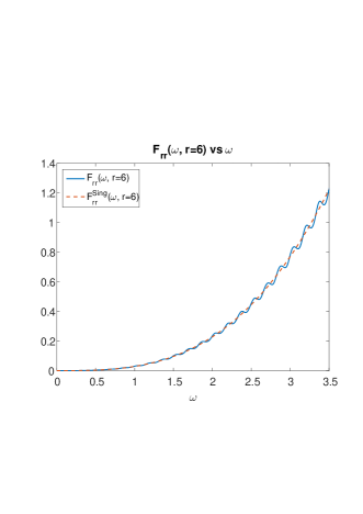
(a) The solid line is the numerically calculated $F_{rr}\left(\omega,r=6\right)$; it is proportional to $\omega^{3}$ for large $\omega$ and clearly divergent. The dashed line is the analytically computed singular part, $F_{rr}^{Sing}\left(\omega,r=6\right)$, which captures the non-oscillatory divergent part of $F_{rr}\left(\omega,r=6\right)$.

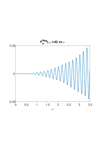
(b) The result of subtracting the singular part $F_{rr}^{Sing}\left(\omega,r=6\right)$ from $F_{rr}\left(\omega,r=6\right)$, which is the definition of $F_{rr}^{Reg}\left(\omega,r=6\right)$ in Eq. (16). It is dominated by oscillations with an amplitude proportional to $\omega^{5/2}$.

Figure 1:

The generalized integral over $F_{rr}^{Reg}\left(\omega,r=6\right)$ now converges, but it is clear that the regular integral does not. To compute the generalized integral we employ the self-cancellation technique that was presented in Levi =000026 Ori - 2015 - t splitting regularization , and is also discussed in App. A. We first compute the regular integral function

$$H_{rr}\left(\omega,r\right)=\int_{0}^{\omega}F_{rr}^{Reg}\left(\omega^{\prime},r\right)d\omega^{\prime},$$

which can be observed in Fig. 2a for $r=6$. It is now possible to remove the oscillations by applying the self-cancellation operator $T_{*}$, following Eq. (31) one can define

$$H_{rr}^{*}\left(\omega,r\right)\equiv T_{*}\left[H_{rr}\left(\omega,r\right)\right].$$

According to the self-cancellation technique the generalized integral over $F_{rr}^{Reg}\left(\omega,r\right)$ is equivalent to the limit $\omega\to\infty$ of $H_{rr}^{*}\left(\omega,r\right)$. Figure 2b displays $H_{rr}^{*}\left(\omega,r=6\right)$ and it is clear that it has a defined limit as $\omega\to\infty$, and that it converges to this limit rapidly. Notice that we have started with a quantity ($F_{rr}\left(\omega,r=6\right)$) with a magnitude of about unit value, and after subtractions and self-cancellations obtained a result ($H_{rr}^{*}\left(\omega,r=6\right)$) of the order of about $10^{-7}$. This is a great demonstration of the many orders of accuracy lost in the regularization process. This loss of accuracy turns the computation of the RSET into a difficult task, and requires the initial modes to be computed with a very high accuracy. The loss of accuracy is the cause of the numerical deviations at large $\omega$ in $H_{rr}^{*}\left(\omega,r=6\right)$ which are visible in Fig. 2b. To handle this inaccuracy we have built an algorithm that picks the optimal $\omega$ for evaluating the limit $\omega\to\infty$. The chosen value is marked in Fig. 2b by a cross.

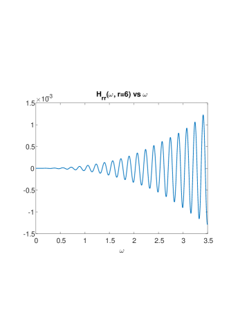
(a) The integral function $H_{rr}\left(\omega,r=6\right)$ vs $\omega$. The amplitude of the oscillations is proportional to $\omega^{5/2}$.

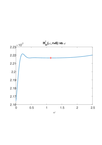
(b) $H_{rr}^{*}\left(\omega,r=6\right)$ vs $\omega$, obtained by applying self-cancellation on $H_{rr}\left(\omega,r=6\right)$. Notice the quick convergence and also the numerical deviations at $\omega\gtrsim 1.5$. The red cross denotes the point chosen by an algorithm we designed to pick the optimal $\omega$ value to estimate the $\omega\to\infty$ limit.

Figure 2:

Following Eq. 18, if we subtract from the limit of $H_{rr}^{*}\left(\omega,r=6\right)$ the term $e_{rr}\left(r=6\right)$ we get $\left\langle\tilde{T}{}_{\mu\nu}\left(r=6\right)\right\rangle_{ren}$ (in units of $\hbar$). Repeating the scheme described above for different $r$ values, and for all the non-trivial components of the RSET we computed $\left\langle\tilde{T}{}_{\mu\nu}\left(r\right)\right\rangle_{ren}$. Simply by trace-reversing this result we obtained $\left\langle T_{\mu\nu}\left(r\right)\right\rangle_{ren}$. Figure 3 presents the results for the RSET, for all the non-trivial components ($T_{t}^{\,t},T{}_{r}^{\,r},T{}_{\theta}^{\,\theta}=T{}_{\varphi}^{\,\varphi}$). For reference we also plot results by Paul Anderson, obtained using the traditional regularization method in the Euclidean sector Anderson - 1995 - Tab static spherically symmetric . We note that we also computed the RSET using the angular-splitting and the agreement between the two is usually a few parts in $10^{3}$.

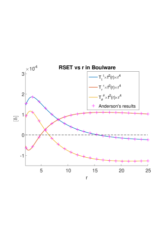
Figure 3: The solid curves represent the RSET in the Boulware state, calculated using the $t$-splitting variant. The plus symbols are results by Paul Anderson, obtained using the traditional regularization method Anderson - 1995 - Tab static spherically symmetric . The RSET in the Boulware state is divergent at the horizon, and decays at infinity like $r^{-4}$. To clarify the picture we multiplied the components by factors of $f\left(r\right)\equiv 1-2M/r$ and $r$.

IV.1 Unruh and Hartle-Hawking states

Due to the fact that our method does not resort to the Euclidean sector, the regularization process is exactly the same for all quantum states. Thus in order to compute a different quantum state one only needs to insert the solution for the modes in this particular state. In the Schwarzschild example the two states that are physically interesting, apart from the Boulware state, are the Unruh and Hartle-Hawking states. Conveniently, in the Schwarzschild case one is not required to recalculate the modes, and can build the the mode-sum in the Unruh and Hartle-Hawking states using the modes of the Boulware state $f_{\omega lm}^{in}\left(x\right),\,f_{\omega lm}^{up}\left(x\right)$ Christensen and Fulling . In our notation it can be written as

$$F_{\mu\nu}^{Unruh}\left(\omega,x\right)=\sum_{l=0}^{\infty}\sum_{m=-l}^{l}\Re\left\{f_{\omega lm,\mu}^{in}\left(x\right)f_{\omega lm,\nu}^{in*}\left(x\right)+\coth\left(\frac{\pi\omega}{\kappa}\right)f_{\omega lm,\mu}^{up}\left(x\right)f_{\omega lm,\nu}^{up*}\left(x\right)\right\}.$$

$$F_{\mu\nu}^{H-H}\left(\omega,x\right)=\sum_{l=0}^{\infty}\sum_{m=-l}^{l}\coth\left(\frac{\pi\omega}{\kappa}\right)\Re\left\{f_{\omega lm,\mu}^{in}\left(x\right)f_{\omega lm,\nu}^{in*}\left(x\right)+f_{\omega lm,\mu}^{up}\left(x\right)f_{\omega lm,\nu}^{up*}\left(x\right)\right\}.$$

Using these relations we have calculated the RSET in the Unruh and Hartle-Hawking states. Note that the regularization scheme remains the same, because the counter-term is independent of the quantum state. Figure 4 presents the results for the Unruh state and Fig. 5 the results for the Hartle-Hawking state. In both states we have crossed our results by computing the RSET in a different method, the angular-splitting variant Levi =000026 Ori - 2016 - theta splitting regularization . In Unruh the two variants agree to about one part in $10^{3}$, and in Hartle-Hawking the deviation is about one part in $10^{4}$. In the Unruh state there is also a non-vanishing flux component $T_{t}^{r}$, which represents the Hawking radiation. We computed the total luminosity to be $L\equiv-4\pi r^{2}T_{t}^{r}\cong 7.4388\cdot 10^{-5}\hbar M^{-2}$, in full agreement with the result by Elster Elster .

Figure 4: The RSET in the Unruh state. Here the RSET is finite on the horizon and we multiply by $f\left(r\right)\equiv 1-2M/r$ to treat the coordinate singularity. Note that $-r^{2}T_{t}^{r}$ is a conserved quantity, representing the outgoing Hawking radiation to infinity.

Figure 5: The RSET in the Hartle-Hawking state. Here the RSET is finite at the horizon, and the multiplication by $f\left(r\right)\equiv 1-2M/r$ is for scaling purposes only.

V Discussion

We have presented the details of the RSET computation for stationary, asymptotically-flat backgrounds, using the $t$-splitting variant of the PMR method. Results were given for the Schwarzschild background in all vacuum states for a minimally-coupled, massless scalar field. We have also demonstrated that many orders of magnitude of accuracy are lost in the computation, which requires the original modes to be computed very accurately in order to obtain a good evaluation of the RSET (see Sec. IV).

Although the scheme was presented here for a minimally-coupled, massless scalar field, it can also be implemented for other fields. For example, one can use the same technique on Christensen’s tensor for an electromagnetic field, which can be found in Christensen 1978 . In addition we have presented the method using Christensen’s scheme and counter terms, but one can also implement it to the Hadamard regularization approach Wald - Hadamrad regularization , where it can also be extended to higher dimensions (similar to Ref. Peter taylor ).

An important issue regarding the $t$-splitting variant is to understand where it is expected to break down. We do not go into deep investigation of this point, and merely state that the scheme breaks down where the norm of the Killing field vanishes. For example, in Schwarzschild $t$-splitting does not work on the horizon. Furthermore, the scheme does not break dichotomically, rather, it becomes less efficient on approaching the locus where the norm vanishes. By less efficient we mean that it requires a larger number of modes, namely a larger $l_{max}$ for the convergence of the sum, and a larger $\omega_{max}$ for the convergence of the integral. For example, in Schwarzschild we used $t$-splitting to approached the horizon up to $r=2.05M$.

Another important aspect of the $t$-splitting is the different techniques for treating the oscillations. In App. A we discussed different techniques that we have explored and were not mentioned in Ref. Levi =000026 Ori - 2015 - t splitting regularization . We believe that one can think of other techniques to implement the generalized integral. As these techniques will become more efficient the number of modes required for regularization will decrease and computation will become easier. One such approach that we have not tested yet is studying the oscillations using the global Hadamard form. Such global function was recently found for the Schwarzschild case by Casals and Nolan Casals =000026 Nolan - Global Hadamrd function . We hope that future work will enable to study the global Hadamard function for more generic backgrounds.

The $t$-splitting presented here was already used to compute $\left\langle\phi^{2}\right\rangle_{ren}$ and the RSET in the exterior region of Kerr Levi Eilon Ori and DeMeent - 2016 - Kerr , yet we believe that there are many more implications for it. Possible extensions of the current work in Kerr spacetime are to compute the RSET inside the ergosphere and inside the horizon. In addition, the method can be used to study other interesting stationery backgrounds such as compact, rapidly spinning stars.

Other implementations of the PMR method, including the details of how to compute the RSET using the angular-splitting variant, and the details of the $\varphi$-splitting variant will be given elsewhere Preparation . Furthermore, we think that the different PMR variants can be improved further in the future to create more efficient schemes, without demanding more symmetries.

Appendix A Oscillations, generalized integrals, and self-cancellation

This appendix briefly summarizes the broad discussion in Levi =000026 Ori - 2015 - t splitting regularization regarding the oscillations in the mode sum. As explained there these oscillations are caused by singularities in the TPF which are not at the coincidence limit. Rather, these singularities correspond to connecting null geodesics (CNGs) Kay Radzikowski and Wald - 1996 , and by computing the CNGs of the background metric one can compute the wavelengths of the oscillations.

Analytically the oscillations are not a problem at all, as our integral is a generalized integral. One way to define a generalized integral over a function $h\left(\omega\right)$ is taking the limit of a Laplace transform

$$\lim_{\alpha\to 0^{+}}\int_{0}^{\infty}h\left(\omega\right)e^{-\alpha\omega}d\omega.$$

But this is very hard to perform numerically. To this purpose we have introduced the self cancellation technique, which enables one to compute the generalized integral for the case of a function with oscillations, given that the wavelengths of the oscillations are known. For example, if one wants to compute the generalized integral over $h\left(\omega\right)$, which apart from a regularly convergent part contains an oscillatory term of the type $\cos\left(\frac{2\pi}{\lambda}\omega\right)$, than by first computing the standard integral function

$$H\left(\omega \right)={\int }_0^{\omega }h\left({\omega }^{\prime }\right)𝑑{\omega }^{\prime },$$

References

- (1) S. W. Hawking, Commun. Math. Phys. 43, 199 (1975).
- (2) B. S. DeWitt, Dynamical Theory of Groups and Fields (Gordon and Breach, New York, 1965).
- (3) J. Schwinger, Phys. Rev. 82, 664 (1951).
- (4) S. M. Christensen, Phys. Rev. D 14, 2490 (1976).
- (5) P. Candelas, Phys. Rev. D 21, 2185 (1980).
- (6) P. Candelas and K. W. Howard, Phys. Rev. D 29, 1618 (1984).
- (7) K. W. Howard, Phys. Rev. D 30, 2532 (1984).
- (8) P. R. Anderson, Phys. Rev. D 41, 1152 (1990).
- (9) P. R. Anderson, W. A. Hiscock, and D. A. Samuel, Phys. Rev. D 51, 4337 (1995).
- (10) P. Taylor and C. Breen, Phys. Rev. D 94, 125024 (2016).
- (11) A. Levi and A. Ori, Phys. Rev. D 91, 104028 (2015).
- (12) A. Levi and A. Ori, Phys. Rev. D 94, 044054 (2016).
- (13) A. Levi and A. Ori, Phys. Rev. Lett. 117, 231101 (2016).
- (14) A. Levi, E. Eilon, A. Ori and M. van de Meent, arXiv:1610.04848.
- (15) A. Levi and A. Ori (In preparation).
- (16) S. M. Christensen, Phys. Rev. D 17, 946 (1978).
- (17) S. M. Christensen and S. A. Fulling, Phys. Rev. D 15, 2088 (1977).
- (18) T. Elster, Phys. Lett. 94 A, 205 (1983).
- (19) R. M. Wald, Commun. Math. Phys. 54, 1 (1977).
- (20) M. Casals and B. Nolan, arXiv:1606.03075.
- (21) B. S. Kay, M. J. Radzikowski and R. M. Wald, Commun. Math. Phys. 183, 533 (1997).