Abstract

We revisit the minimal seesaw model, i.e., the type-I seesaw mechanism involving only two right-handed neutrinos. This model represents an important minimal benchmark scenario for future experimental updates on neutrino oscillations. It features four real parameters that cannot be fixed by the current data: two $CP$-violating phases, $\delta$ and $\sigma$, as well as one complex parameter, $z$, that is experimentally inaccessible at low energies. The parameter $z$ controls the structure of the neutrino Yukawa matrix at high energies, which is why it may be regarded as a label or index for all UV completions of the minimal seesaw model. The fact that $z$ encompasses only two real degrees of freedom allows us to systematically scan the minimal seesaw model over all of its possible UV completions. In doing so, we address the following question: Suppose $\delta$ and $\sigma$ should be measured at particular values in the future—to what extent is one then still able to realize approximate textures in the neutrino Yukawa matrix? Our analysis, thus, generalizes previous studies of the minimal seesaw model based on the assumption of exact texture zeros. In particular, our study allows us to assess the theoretical uncertainty inherent to the common texture ansatz. One of our main results is that a normal light-neutrino mass hierarchy is, in fact, still consistent with a two-zero Yukawa texture, provided that the two texture zeros receive corrections at the level of $\mathcal{O}\left(\textrm{10}\,\%\right)$. While our numerical results pertain to the minimal seesaw model only, our general procedure appears to be applicable to other neutrino mass models as well.

1 Intro: Possible lessons from measuring leptonic $CP$ violation?

After the celebrated discovery of neutrino masses and mixings during the last two decades [1], current and upcoming neutrino experiments are now on the brink of taking the next big step: the observation of $CP$ noninvariance in neutrino oscillations [2]. Theory predicts that such leptonic $CP$ violation manifests itself in at least one nonvanishing phase, $\delta$, in the lepton mixing matrix [3]; and ongoing long-baseline experiments such as NO$\nu$A [4] and T2K [5] prove to become increasingly sensitive to this observable. Recently, the NO$\nu$A collaboration, e.g., reported their newest constraints on the $CP$-violating phase $\delta$ [6], which illustrate that NO$\nu$A is now capable of excluding certain values of $\delta$ at the level of $3\,\sigma$. Moreover, planned long-baseline experiments such as DUNE [7] will be able to actually measure $\delta$ over a large range of possible values.

From the viewpoint of theory, these recent developments as well as experimental prospects directly lead to the question: What can we possibly learn about the properties of the Standard Model (SM) neutrinos from measuring a certain amount of $CP$ violation in neutrino oscillations? In this paper, we are going to attempt to answer this question in the context of the minimal seesaw model, i.e., the type-I seesaw mechanism [8] including only two right-handed neutrinos.

The seesaw mechanism is arguably one of the most popular explanations of the SM neutrino masses. At the cost of a minimal extension of the SM particle content, it manages to account for all observed low-energy neutrino phenomena, while in addition offering the possibility to explain the baryon asymmetry of the universe as a consequence of baryogenesis via leptogenesis [9]. Traditionally, the seesaw mechanism supposes the existence of three right-handed neutrinos, $N_{I}$ with $I=1,2,3$, that transform as complete singlets under the SM gauge group. In this standard scenario, all three SM neutrinos acquire small nonvanishing masses, the differences between which are then described by the observed solar and atmospheric mass-squared differences, $\Delta m_{\rm sol}^{2}$ and $\Delta m_{\rm atm}^{2}$. This realization of the seesaw mechanism, however, comes with a large number of undetermined parameters at high energies, which makes it difficult to derive distinct predictions for the neutrino observables accessible at low energies. A possible way out of this problem is to assume certain (discrete) flavor symmetries that restrict the set of allowed leptonic interactions in the Lagrangian, thereby reducing the number of free parameters [10]. This approach is well motivated and has attracted (and continues to attract) a great deal of attention in the literature. On the other hand, the concept of flavor symmetries often times requires a large number of additional scalar fields in order to achieve certain Yukawa structures. This increases the particle content and, hence, overall complexity of the seesaw mechanism at high energies, which may make it even harder to experimentally pin down its underlying dynamics at a fundamental level.

An intriguing and, in fact, quite orthogonal alternative to this approach is to simply reduce the number of right-handed neutrinos from three to two [11, 12]. In this case, one has to deal with three complex Yukawa couplings or, equivalently, six real parameters less. As a consequence, one SM neutrino remains massless, while the masses of the other two neutrinos are readily fixed by $\Delta m_{\rm sol}^{2}$ and $\Delta m_{\rm atm}^{2}$. This realization of the seesaw mechanism is, thus, significantly more predictive than the standard scenario involving three right-handed neutrinos. In addition, it nicely conforms with the philosophy of Occam’s razor [13], which commands us to always give preference to explanations that rely on the least number of assumptions. To explain the current low-energy neutrino data, one actually does not need to introduce three right-handed neutrinos. Lacking knowledge of the absolute neutrino mass scale, two right-handed neutrinos are absolutely sufficient. Likewise, leptogenesis calls for two right-handed neutrinos, but not necessarily more [12, 14]. Two (nondegenerate) right-handed neutrinos are sufficient to render the decays of the heavy $N_{I}$ in the early universe $CP$-noninvariant, as required by the Sakharov conditions for successful baryogenesis [15]. A third right-handed neutrino is not essential. In fact, as recently shown explicitly in Ref. [16], the type-I seesaw mechanism with only two right-handed neutrinos succeeds in reproducing the observed baryon asymmetry of the universe via resonant leptogenesis [17], i.e., for a nearly degenerate heavy-neutrino mass spectrum. Taking into account arguments from electroweak naturalness, the authors of Ref. [16] find that the two heavy neutrinos in the minimal seesaw model should have a similar mass, not much larger than $\mathcal{O}\left(10^{7}\right)\,\textrm{GeV}$. In view of this result, we shall focus on more or less similar heavy-neutrino masses in the following, neglecting the possibility of a strongly hierarchical spectrum.

In the case of two rather than three right-handed neutrinos, the SM Lagrangian needs to be supplemented with the following Yukawa and mass terms at high energies,

$$\mathcal{L}_{\rm seesaw}=-y_{\alpha I}\,\ell_{\alpha}N_{I}H-\frac{1}{2}\,M_{I}N_{I}N_{I}+\textrm{h.c.}\,,\quad\alpha=e,\mu,\tau\,,\quad I=1,2\,.$$ (1)

Here, the first term accounts for the Yukawa interactions of the right-handed neutrinos with the SM lepton and Higgs doublets, $\ell_{\alpha}=\left(\nu_{\alpha},e_{\alpha}\right)^{T}$ and $H=\left(H^{+},H^{0}\right)^{T}$, while the second term contains Majorana masses, $M_{I}$, for the right-handed neutrinos, which, w.l.o.g., we can take to be real and diagonal. Meanwhile, the Yukawa couplings $y_{\alpha I}$ form an arbitrary complex $3\times 2$ matrix. The main goal of this paper will be to study the implications for the Yukawa matrix $y_{\alpha I}$, provided that leptonic $CP$ violation should be conclusively observed in the future.

General seesaw models involving three right-handed neutrinos predict the existence of, in total, three physical $CP$-violating phases in the lepton mixing matrix: one Dirac phase $\delta$, which is always present and which may be regarded as the analog of the complex phase in the quark mixing matrix [19], as well as two additional phases, $\sigma$ and $\tau$, owing to the Majorana nature of the SM neutrinos in the context of seesaw models. In the case of only two right-handed neutrinos, one of these two Majorana phases (say, $\tau$) can, however, be absorbed by a neutrino field rotation, so that only two phases end up being physical: $\delta$ and $\sigma$. Here, $\delta$ can be measured in neutrino oscillation experiments, while $\sigma$ enters into the effective neutrino masses probed in searches for neutrinoless double-beta decay (such as GERDA [20]) or in experiments aiming at a direct neutrino mass determination (such as KATRIN [21]). In this paper, we are now going to study the possible hierarchy structures and textures in the Yukawa matrix $y_{\alpha I}$ in dependence of the $CP$-violating phases $\delta$ and $\sigma$. To this end, we will adopt a two-step strategy: First, we will introduce a convenient measure that characterizes how close a given Yukawa matrix is to a certain flavor texture. Then, we will perform a systematic parameter scan of the model in Eq. (1) and maximize, for fixed values of $\delta$ and $\sigma$, our hierarchy parameter over all the unconstrained parameters that are inaccessible to low-energy experiments. This will allow us to assess how strong a hierarchy between different Yukawa couplings one could possibly realize for any given values of $\delta$ and $\sigma$. Our hope is that such a phenomenological link between experimentally accessible observables on the one hand and fundamental theory parameters on the other hand may help shed more light on the underlying dynamics of the seesaw mechanism and on the UV origin of its flavor structure. Our approach covers, in particular, all viable UV completions of the minimal seesaw model from a bottom-up phenomenological perspective.

Our analysis ties in with studies of the minimal seesaw model that assume exact texture zeros in the neutrino Yukawa matrix [12, 22, 23, 24]. Such exact zeros may occur in consequence of certain flavor symmetries in the fundamental high-energy theory of flavor. Moreover, they comply with the spirit of Occam’s razor and, thirdly, they have proven to be a successful phenomenological tool in the quark sector in the past. As shown by Weinberg [25], imposing texture zeros in the mass matrices for the first two quark generations allows one to derive a successful prediction for the Cabibbo angle, $\theta_{C}=\left(m_{d}/m_{s}\right)^{1/2}\simeq 0.22$. The main difference between our analysis and the “texture ansatz” is that we intend to tackle the flavor problem in the neutrino sector from quite the opposite direction. The philosophy behind neutrino mass models involving texture zeros is to derive phenomenological predictions from a more or less well motivated choice of Yukawa couplings at high energies. This amounts to a classical top-down approach. When confronted with the experimental data, such models typically lead to an all-or-nothing situation: Either the data turns out to be consistent with the model’s predictions or the model is ruled out. We, by contrast, remain a priori agnostic as to the structure of the neutrino Yukawa matrix and let the data decide what hierarchies or textures are experimentally preferred or ruled out. In this sense, we are going to pursue a data-driven bottom-up approach, which offers an interesting and conceptually new perspective on the interplay between experimental and theoretical progress. As we do not impose any conditions on the neutrino Yukawa couplings from the outset, our approach is considerably more model-independent than the conventional theory-driven texture ansatz. Or in other words, we no longer put all our eggs into one basket. With the data being the driving force behind our analysis, any future data update, if interpreted in the context of the minimal seesaw model, is guaranteed to provide us with new insights regarding possible UV completions of the two-right-handed-neutrino model, see also Fig. 7 in the Conclusions (Sec. 6).

The rest of the paper is organized as follows. In the next section, we shall first review the type-I seesaw mechanism featuring two right-handed neutrinos. In Sec. 3, we will then define our novel hierarchy parameter that will allow us to quantify the quality of different hierarchies in the neutrino Yukawa matrix. Subsequently, we will present in Sec. 4 the results of our scan of parameter space, i.e., the maximal hierarchy parameter in dependence of $\delta$ and $\sigma$. Here, our main conclusion will be that models with two right-handed neutrinos and approximate two-zero textures can still accommodate both a normal (NH) and an inverse (IH) neutrino mass hierarchy. This represents an important caveat to the conventional statement that seesaw models with two right-handed neutrinos and two texture zeros do not allow for a normally ordered light-neutrino mass spectrum. Similarly, we will show how, in the case of an inverse mass hierarchy, the viable set of exact textures can be generalized to a much larger set of approximate textures. Most of our observations are in accord with the naive expectation that relaxing the assumption of an exact flavor texture should enlarge the accessible part of parameter space. But to us, it seems as if our approach presents the issue of Yukawa hierarchies in minimal neutrino mass models from a new angle and, thus, deserves a closer examination. In a sense, it may be regarded as a supplement to all minimal seesaw models that assume exact texture zeros in the neutrino Yukawa matrix. If one thinks of the predictions of these models as “central values” of a sort, our analysis yields the corresponding “theoretical error bars” to these predictions. In Sec. 5, we will briefly discuss the stability of our numerical results under variations in the experimental input data. As we will see, our findings for $\delta$ and $\sigma$ exhibit an absolute uncertainty owing to the experimental errors of at most $\mathcal{O}\left(1\,\%\right)\pi$. In Sec. 6, we will finally conclude and give a brief outlook as to how our analysis could be extended. We will comment on the possibility of generalizing our analysis to arbitrary textures as well as to the case of three right-handed neutrinos.

2 Type-I seesaw mechanism with two right-handed neutrinos

Let us first recall how the seesaw Lagrangian in Eq. (1) results in small Majorana masses for the SM neutrinos. In the course of electroweak symmetry breaking, the Higgs field $H^{0}$ acquires a nonvanishing vacuum expectation value (VEV), $v_{\rm ew}\simeq 174\,\textrm{GeV}$. This turns the Yukawa term in Eq. (1) into a Dirac mass term for the left-handed and right-handed neutrinos $\nu_{\alpha}$ and $N_{I}$,

$$\mathcal{L}_{\rm seesaw}=-\left(m_{D}\right)_{\alpha I}\,\nu_{\alpha}N_{I}-\frac{1}{2}\,M_{I}N_{I}N_{I}+\textrm{h.c.}\,,\quad\left(m_{D}\right)_{\alpha I}=y_{\alpha I}\,v_{\rm ew}\,.$$ (2)

Provided there is a strong hierarchy between the Dirac and Majorana mass terms, $M_{I}\gg\left(m_{D}\right)_{\alpha I}$, the right-handed neutrinos $N_{I}$ decouple at low energies, such that we can integrate them out. This results in the famous type-I seesaw formula for the SM neutrino masses,

$$\mathcal{L}_{\rm seesaw}=-\left(m_{\nu}\right)_{\alpha\beta}\,\nu_{\alpha}\nu_{\beta}+\textrm{h.c.}\,,\quad\left(m_{\nu}\right)_{\alpha\beta}=-v_{\rm ew}^{2}\,y_{\alpha I}\,M_{I}^{-1}\,y_{\beta I}\,.$$ (3)

Here, the SM neutrino mass matrix, $\left(m_{\nu}\right)_{\alpha\beta}$, is a complex symmetric $3\times 3$ matrix, which needs to be diagonalized by a unitary Takagi factorization. In matrix notation, this means

$$D_{\nu}=U^{T}\,m_{\nu}\,U\,,\quad D_{\nu}=\textrm{diag}\left\{m_{1},m_{2},m_{3}\right\}\,.$$ (4)

For a normally ordered light-neutrino mass spectrum, we have $m_{1}<m_{2}<m_{3}$, whereas an inversely ordered light-neutrino mass spectrum is characterized by $m_{3}<m_{1}<m_{2}$. In the presence of only two right-handed neutrinos, $\left(m_{\nu}\right)_{\alpha\beta}$ in Eq. (3) is a rank-2 matrix. The lightest neutrino mass eigenvalue therefore vanishes in our model for both NH and IH, $\min\left\{m_{i}\right\}=0$.

We shall work in a basis in which the charged-lepton mass matrix is diagonal. Then we can identify the unitary matrix $U$ in Eq. (4) as the lepton mixing or Pontecorvo-Maki-Nakagawa-Sakata (PMNS) matrix, which relates the flavor eigenstates $\nu_{\alpha}$ to the mass eigenstates $\nu_{i}$,

$$\nu_{\alpha}=U_{\alpha i}\,\nu_{i}\,,\quad\nu_{i}=U_{\alpha i}^{*}\,\nu_{\alpha}\,,\quad\alpha=e,\mu,\tau\,,\quad i=1,2,3\,.$$ (5)

In the case of one massless SM neutrino, the PMNS matrix encompasses five (instead of the usual six) physical degrees of freedom (DOFs): three mixing angles, $\theta_{12}$, $\theta_{13}$, and $\theta_{23}$, which take values in the interval $[0,\pi/2]$, as well as two $CP$-violating phases, $\delta\in\left[0,2\pi\right)$ and $\sigma\in\left[0,\pi\right)$,

$$U=\begin{pmatrix}c_{12}\,c_{13}&s_{12}\,c_{13}&s_{13}\,e^{-i\delta}\\ -s_{12}\,c_{23}-c_{12}\,s_{13}\,s_{23}\,e^{i\delta}&\phantom{-}c_{12}\,c_{23}-s_{12}\,s_{13}\,s_{23}\,e^{i\delta}&s_{23}\,c_{13}\\ \phantom{-}s_{12}\,s_{23}-c_{12}\,s_{13}\,c_{23}\,e^{i\delta}&-c_{12}\,s_{23}-s_{12}\,s_{13}\,c_{23}\,e^{i\delta}&c_{23}\,c_{13}\end{pmatrix}\begin{pmatrix}1&0&0\\ 0&e^{i\sigma}&0\\ 0&0&1\end{pmatrix}\,.$$ (6)

Here, $c_{ij}$ and $s_{ij}$ are a shorthand notation for $\cos\theta_{ij}$ and $\sin\theta_{ij}$, respectively. In total, we, thus, arrive at the conclusion that the SM neutrino sector features seven low-energy observables: the five observables encoded in the PMNS matrix as well as two nonzero mass eigenvalues. This needs to be contrasted with the available parameters at high energies. The neutrino Yukawa matrix $y_{\alpha I}$ contains twelve real parameters—six absolute values and six phases—out of which three phases are unphysical as they can be absorbed by charged-lepton rotations. Meanwhile, the right-handed neutrino masses $M_{1,2}$ constitute two further high-energy parameters. Changes in these masses can, however, be compensated for by a rescaling of the neutrino Yukawa couplings,

$$M_{I}\rightarrow M_{I}^{\prime}\,,\quad y_{\alpha I}\rightarrow\left(\frac{M_{I}^{\prime}}{M_{I}}\right)^{1/2}y_{\alpha I}\,.$$ (7)

This leaves us with, in total, $12-3+2-2=9$ independent parameters at high energies, which is sufficient to account for the seven low-energy observables contained in $D_{\nu}$ and $U$.

The functional relation between the input parameters at high energies and the observables at low energies becomes most transparent in the Casas-Ibarra parametrization of the neutrino Yukawa matrix [27]. To re-derive this parametrization making use of our conventions and notations, we simply have to combine the seesaw formula in Eq. (3) with the relation in Eq. (4),

$$D_{\nu}=-v_{\rm ew}^{2}\,U^{T}\,y\,D_{N}^{-1}\,y^{T}\,U\,,\quad D_{N}=\textrm{diag}\left\{M_{1},M_{2}\right\}\,.$$ (8)

Solving this matrix equation for the neutrino Yukawa matrix, one finds

$$y=\frac{i}{v_{\rm ew}}\,U^{*}D_{\nu}^{1/2}\,R\,D_{N}^{1/2}\,,$$ (9)

where $R$ is a complex $3\times 2$ rotation matrix that satisfies $R^{T}R=\mathbb{1}_{2\times 2}$, but not $RR^{T}=\mathbb{1}_{3\times 3}$,

$$\textrm{NH:}\quad m_{1}=0\,,\quad R=\begin{pmatrix}0&0\\ \cos z&-\sin z\\ \zeta\sin z&\zeta\cos z\end{pmatrix}\,,\quad\textrm{IH:}\quad m_{3}=0\,,\quad R=\begin{pmatrix}\cos z&-\sin z\\ \zeta\sin z&\zeta\cos z\\ 0&0\end{pmatrix}\,.$$ (10)

Here, the rotation angle $z$ is an arbitrary complex number, which represents the two real excess DOFs in the high-energy Yukawa matrix $y_{\alpha I}$ compared to the low-energy mass matrix $\left(m_{\nu}\right)_{\alpha\beta}$. The parameter $\zeta=\pm 1$ distinguishes between a “positive” and a “negative” branch of possible rotation matrices $R$. The resulting Yukawa matrices on both branches can, however, be mapped onto each other by a combination of sign changes, column exchange, etc.; see Appendix B of Ref. [18] for details. For our purposes, we are, thus, free to either pick $\zeta=+1$ or $\zeta=-1$. In the following, we will work, w.l.o.g., with the Yukawa matrices on the positive branch, $\zeta=+1$. The Casas-Ibarra parametrization also exhibits the re-parametrization freedom displayed in Eq. (7). To see this explicitly, it turns out convenient to introduce the following quantities,

$$\kappa_{\alpha I}=-i\,y_{\alpha I}\,\sqrt{\frac{v_{\rm ew}}{M_{I}}}\,,\quad V_{\alpha i}=U_{\alpha i}^{*}\,\sqrt{\frac{m_{i}}{v_{\rm ew}}}\,,$$ (11)

which allow us to write down a dimensionless version of the Casas-Ibarra parametrization,

$$\textrm{NH:}\quad\begin{pmatrix}\kappa_{\alpha 1}\\ \kappa_{\alpha 2}\end{pmatrix}=\begin{pmatrix}\cos z&\sin z\\ -\sin z&\cos z\end{pmatrix}\begin{pmatrix}V_{\alpha 2}\\ V_{\alpha 3}\end{pmatrix}\,,\quad\textrm{IH:}\quad\begin{pmatrix}\kappa_{\alpha 1}\\ \kappa_{\alpha 2}\end{pmatrix}=\begin{pmatrix}\cos z&\sin z\\ -\sin z&\cos z\end{pmatrix}\begin{pmatrix}V_{\alpha 1}\\ V_{\alpha 2}\end{pmatrix}\,.$$ (12)

The expressions on the right-hand sides of these two equations now no longer depend on the heavy-neutrino masses $M_{1,2}$. Instead, these two masses are absorbed in the rescaled Yukawa couplings $\kappa_{\alpha I}\propto y_{\alpha I}M_{I}^{-1/2}$, which are invariant under the scaling transformation in Eq. (7). Note also that this version of the Casas-Ibarra parametrization nicely separates the unknown high-energy input parameters (on the left-hand side) from the low-energy observables that can be measured in experiments (on the right-hand side). As evident from Eq. (12), both sets of quantities are related by a rotation about a complex angle $z$. This angle is physically meaningful at high energies, but appears as an “unphysical” auxiliary parameter at low energies.

An important implication of Eq. (12) is that we can always find values of the complex parameter $z$, such that at least one Yukawa coupling vanishes exactly. In fact, all we have to do is to choose $z$ such that $\tan z$ equals the ratio of two entries in the rescaled PMNS matrix $V_{\alpha i}$,

$$\textrm{NH:}\quad\kappa_{\alpha 1} =0\quad\Rightarrow \mkern-18.0mu\tan z =-\frac{V_{\alpha 2}}{V_{\alpha 3}}\,, \textrm{IH:}\quad\kappa_{\alpha 1} =0\quad\Rightarrow \mkern-18.0mu\tan z =-\frac{V_{\alpha 1}}{V_{\alpha 2}}\,,$$ (13)

$$\kappa_{\alpha 2} =0\quad\Rightarrow \mkern-18.0mu\tan z =+\frac{V_{\alpha 3}}{V_{\alpha 2}}\,, \kappa_{\alpha 2} =0\quad\Rightarrow \mkern-18.0mu\tan z =+\frac{V_{\alpha 2}}{V_{\alpha 1}}\,.$$

Requiring a one-zero texture in the neutrino Yukawa matrix, thus, eliminates the parameter $z$ and leaves us with an equal number of input parameters and observables. Such one-zero texture models have been extensively discussed in the literature [23], more recently in particular in the context of constrained sequential dominance [28]; see, e.g., Ref. [29] and references therein.

Realizing two zeros in the neutrino Yukawa matrix is already more challenging, as it requires a conspiracy among four entries in the rescaled PMNS matrix $V_{\alpha i}$. Schematically, we have

$$\left(\kappa_{\alpha I},\kappa_{\beta J}\right)=\left(0,0\right)\,,\quad\left(\alpha,I\right)\neq\left(\beta,J\right)\quad\Rightarrow\quad\frac{V_{1}}{V_{2}}=\pm\frac{V_{3}}{V_{4}}\,,$$ (14)

with the exact matrix entries $V_{1,2,3,4}$ following from Eq. (13), respectively. In fact, such scenarios correspond to the most minimal realizations of the seesaw mechanism [12, 13]. It is easy to see that, in the case of only two right-handed neutrinos, three or more texture zeros in the neutrino Yukawa matrix lead to at least two vanishing neutrino mixing angles. Therefore, given the fact that all three mixing angles, including the reactor mixing angle $\theta_{13}$, have been measured to be nonzero in experiments in recent years, models with more than two texture zeros clearly conflict with the data. Meanwhile, also models with two texture zeros are highly constrained. To illustrate the range of viable two-zero textures, let us adopt the notation of Ref. [24], which categorizes all possible two-zero textures in the matrix $y_{\alpha I}$ into three groups, $A_{i}$, $B_{i}$, and $C_{i}$,

$$A_{1}\,:\>\begin{pmatrix}0&0\\ \times&\times\\ \times&\times\end{pmatrix}\,,\quad A_{2}\,:\>\begin{pmatrix}\times&\times\\ 0&0\\ \times&\times\end{pmatrix}\,,\quad A_{3}\,:\>\begin{pmatrix}\times&\times\\ \times&\times\\ 0&0\end{pmatrix}\,,$$ (15)

$$B_{1}\,:\>\begin{pmatrix}0&\times\\ \times&0\\ \times&\times\end{pmatrix}\,,\quad B_{2}\,:\>\begin{pmatrix}0&\times\\ \times&\times\\ \times&0\end{pmatrix}\,,\quad B_{3}\,:\>\begin{pmatrix}\times&\times\\ 0&\times\\ \times&0\end{pmatrix}\,,$$

$$B_{4}\,:\>\begin{pmatrix}\times&0\\ 0&\times\\ \times&\times\end{pmatrix}\,,\quad B_{5}\,:\>\begin{pmatrix}\times&0\\ \times&\times\\ 0&\times\end{pmatrix}\,,\quad B_{6}\,:\>\begin{pmatrix}\times&\times\\ \times&0\\ 0&\times\end{pmatrix}\,,$$

$$C_{1}\,:\>\begin{pmatrix}0&\times\\ 0&\times\\ \times&\times\end{pmatrix}\,,\quad C_{2}\,:\>\begin{pmatrix}0&\times\\ \times&\times\\ 0&\times\end{pmatrix}\,,\quad C_{3}\,:\>\begin{pmatrix}\times&\times\\ 0&\times\\ 0&\times\end{pmatrix}\,,$$

$$C_{4}\,:\>\begin{pmatrix}\times&0\\ \times&0\\ \times&\times\end{pmatrix}\,,\quad C_{5}\,:\>\begin{pmatrix}\times&0\\ \times&\times\\ \times&0\end{pmatrix}\,,\quad C_{6}\,:\>\begin{pmatrix}\times&\times\\ \times&0\\ \times&0\end{pmatrix}\,.$$

As shown in Refs. [13, 24], only four out of these 15 textures turn out to be compatible with the current low-energy neutrino data: $B_{1}$, $B_{2}$, $B_{4}$, and $B_{5}$—and that even only in the case of an inverse mass hierarchy. This amounts to the statement that the type-I seesaw model with two right-handed neutrinos and an exact two-zero texture does not allow for a normally ordered light-neutrino mass spectrum. Of course, this conclusion no longer holds true once one gives up on the texture zeros in Eq. (15) and replaces all zeros by nonzero entries. One of our main goals in this paper will be to quantify this statement and to assess how large these corrections to an exact two-zero texture need to be so that a normal mass hierarchy comes into reach again. Moreover, it is important to note that the pairs of textures $B_{1}$ and $B_{4}$ as well as $B_{2}$ and $B_{5}$ only differ by an exchange of the two columns in $y_{\alpha I}$. Physically, this simply corresponds to the two neutrinos $N_{1}$ and $N_{2}$ interchanging their coupling strengths to the SM lepton-Higgs fields. Such a change in the Yukawa term in Eq. (1) can, however, always be compensated for by a corresponding change in the $N_{1,2}$ Majorana masses, $M_{1}\leftrightarrow M_{2}$. The textures $B_{1,4}$ and $B_{2,5}$ are, thus, bound to lead to the same low-energy predictions, respectively. This is best seen in the predictions for the $CP$-violating phases $\delta$ and $\sigma$. Owing to the restrictive condition in Eq. (14), these two observables are completely determined by the neutrino masses and mixings angles. To leading order in the small mixing angle $s_{13}$, one finds [24]

$$\cos\delta\simeq\begin{cases}+\frac{\sin 2\theta_{12}\left(1-m_{1}^{2}/m_{2}^{2}\right)}{4\tan\theta_{23}\sin\theta_{13}}-\frac{\tan\theta_{23}\sin\theta_{13}}{\tan 2\theta_{12}}\\ -\frac{\sin 2\theta_{12}\left(1-m_{1}^{2}/m_{2}^{2}\right)}{4\cot\theta_{23}\sin\theta_{13}}+\frac{\cot\theta_{23}\sin\theta_{13}}{\tan 2\theta_{12}}\end{cases}\,,\quad\cos 2\sigma\simeq\begin{cases}1-\frac{\tan^{2}\theta_{23}\sin^{2}\theta_{13}}{2\sin^{2}\theta_{12}\cos^{2}\theta_{12}}&\quad\left(B_{1,4}\right)\\ 1-\frac{\cot^{2}\theta_{23}\sin^{2}\theta_{13}}{2\sin^{2}\theta_{12}\cos^{2}\theta_{12}}&\quad\left(B_{2,5}\right)\end{cases}\,.$$ (16)

Observable	Units	Hierarchy	Best-fit value	$3\,\sigma$ confidence interval
$\delta m^{2}$	$\left[10^{-5}\,\textrm{eV}^{2}\right]$	both	$+7.37$	$\left[+6.93,+7.97\right]$
$\Delta m^{2}$	$\left[10^{-3}\,\textrm{eV}^{2}\right]$	NH	$+2.50$	$\left[+2.37,+2.63\right]$
		IH	$-2.46$	$\left[-2.33,-2.60\right]$
$\sin^{2}\theta_{12}$	$\left[10^{-1}\right]$	both	$+2.97$	$\left[+2.50,+3.54\right]$
$\sin^{2}\theta_{13}$	$\left[10^{-2}\right]$	NH	$+2.14$	$\left[+1.85,+2.46\right]$
		IH	$+2.18$	$\left[+1.86,+2.48\right]$
$\sin^{2}\theta_{23}$	$\left[10^{-1}\right]$	NH	$+4.37$	$\left[+3.79,+6.16\right]$
		IH	$+5.69$	$\left[+3.83,+6.37\right]$
$\delta$	$\left[\pi\right]$	NH	$+1.35$	$\left[+0.00,+2.00\right]$
		IH	$+1.32$	$\left[+0.00,+2.00\right]$

Table 1: Best-fit values and $3\,\sigma$ confidence intervals for the five low-energy observations that are currently accessible in experiments ($\delta m^{2}$, $\Delta m^{2}$, $\sin^{2}\theta_{12}$, $\sin^{2}\theta_{13}$, and $\sin^{2}\theta_{23}$) as well as for the $CP$-violating phase $\delta$ [31]. Note that, at the $3\,\sigma$ level, $\delta$ can still freely vary over the entire range of possible values, $\delta\in\left[0,2\pi\right)$.

These predictions can be evaluated by making use of the experimental results for the observed masses and mixings. Among the various global-fit results in the literature [30, 31], we shall use the most recent analysis [31] in this paper, for definiteness. Ref. [31] uses the global neutrino data from several neutrino observatories, accelerators and reactors to constrain six observables: $\delta m^{2}$, $\Delta m^{2}$, $\sin^{2}\theta_{12}$, $\sin^{2}\theta_{13}$, $\sin^{2}\theta_{23}$, and $\delta$. Here, the two mass-squared differences $\delta m^{2}$ and $\Delta m^{2}$ correspond to more accurately defined versions of $\Delta m_{\rm sol}^{2}$ and $\Delta m_{\rm atm}^{2}$, respectively,

$$\delta m^{2}=m_{2}^{2}-m_{1}^{2}\,,\quad\Delta m^{2}=m_{3}^{2}-\frac{1}{2}\left(m_{2}^{2}+m_{1}^{2}\right)\,.$$ (17)

Given that, in our scenario, $m_{1}=0$ in the NH case and $m_{3}=0$ in the IH case, the three light-neutrino masses $m_{1,2,3}$ can then be uniquely expressed in terms of $\delta m^{2}$ and $\Delta m^{2}$ as follows,

$$\textrm{NH:}\quad m_{1} =0\,, \textrm{IH:}\quad m_{1} =\left(-\Delta m^{2}-\frac{1}{2}\delta m^{2}\right)^{1/2}\,,$$ (18)

$$m_{2} =\left(\delta m^{2}\right)^{1/2}\,, m_{2} =\left(-\Delta m^{2}+\frac{1}{2}\delta m^{2}\right)^{1/2}\,,$$

$$m_{3} =\left(\Delta m^{2}+\frac{1}{2}\delta m^{2}\right)^{1/2}\,, m_{3} =0\,.$$

Here, note that the sign of $\Delta m^{2}$ is not fixed: $\Delta m^{2}>0$ for NH and $\Delta m^{2}<0$ for IH. The best-fit values as well as $3\,\sigma$ confidence intervals for all six observables are summarized in Tab. 1. With the aid of the best-fit values for $\delta m^{2}$, $\Delta m^{2}$, $\sin^{2}\theta_{12}$, $\sin^{2}\theta_{13}$, and $\sin^{2}\theta_{23}$, we then find the following predictions for the phases $\delta$ and $\sigma$ in models with an exact two-zero texture,

$$\frac{\left(\delta,\sigma\right)}{\pi}\simeq\begin{cases}\left(0.51,0.94\right)\quad\textrm{or}\quad\left(1.49,0.06\right)&\qquad\left(B_{1,4}\right)\\ \left(0.50,0.04\right)\quad\textrm{or}\quad\left(1.50,0.96\right)&\qquad\left(B_{2,5}\right)\end{cases}\,.$$ (19)

A combined determination of $\delta$ and $\sigma$ in experiment (or a sole determination of $\delta$ with a precision at the percent level) would, thus, allow to distinguish between the two possible sets of Yukawa textures. Moreover, it is interesting to observe that both models predict a $CP$-violating phase $\delta$ close to its maximal value, $\delta\simeq\pm\pi/2\>\textrm{mod}\>2\pi$. Remarkably enough, this is in agreement with the (arguably weak) trend in the latest experimental constraints on $\delta$ (see also Ref. [6]).

3 Assessing hierarchies in the neutrino Yukawa matrix

A clear advantage of models with an exact two-zero texture is their testability. If the Yukawa matrix $y_{\alpha I}$ should, indeed, contain two exact zeros, experiments should measure $\delta$ and $\sigma$ at values not much different from those in Eq. (19). However, we are left wondering: What if this should turn out not to be the case? After all, the predictions in Eq. (19) offer us an all-or-nothing perspective: Either experiments determine the phases $\delta$ and $\sigma$ at the predicted values or the minimal seesaw model with two exact texture zeros is immediately ruled out! So, if future data should indicate some deviations from the exact predictions in Eq. (19), should we then abandon the idea of two-zero textures altogether? At this point, we caution that one should not jump to conclusions too quickly. The predictions in Eq. (19) may have experimental error bars (see our analysis in Sec. 5 and, in particular, Fig. 6); but from a theoretical perspective, they are extremely stiff. Not only does this raise the stakes in the all-or-nothing game, it may also appear unnatural for a couple of physical reasons. In reality, the picture of exact texture zeros may very well receive corrections that perturb the naive leading-order neutrino Yukawa matrix. Two exact texture zeros could easily be nothing but a first-order approximation and the matrix $y_{\alpha I}$ may, in fact, rather exhibit a hierarchy structure in the sense that two of its entries are parametrically smaller than the other four. In the high-energy theory of flavor, this may, e.g., be achieved via some sort of explicit flavor symmetry breaking. Alternatively, the texture in the Yukawa matrix may only be exact at tree level and in the absence of gravity, such that radiative and/or gravitational effects might be responsible for small perturbations. In this paper, we will, however, not delve any further into such speculations. Instead, we are going to study the possibility of approximate Yukawa textures from a bottom-up phenomenological point of view. We would like to address the question as to how strong a hierarchy could still be realized in $y_{\alpha I}$, given that $\delta$ and $\sigma$ should be measured at values different from those in Eq. (19). Among other things, this will provide us with theoretical error bars on the predictions in Eq. (19), which we deem useful and relevant not only from a systematic, but also from a physical perspective.

To achieve our goal, we need to compare with each other all possible neutrino Yukawa matrices that lead to the same predictions for $\delta$ and $\sigma$ and find, for each pair of $\left(\delta,\sigma\right)$ values, the most “extreme” matrix that exhibits the strongest hierarchy. Fortunately, such an endeavor is greatly facilitated by the Casas-Ibarra parametrization in Eq. (12). For given values of $\delta$ and $\sigma$, we simply need to evaluate the $V_{\alpha i}$ matrix elements on the right-hand sides of the two relations in Eq. (12). The respective sets of Yukawa couplings that we are interested in then readily follow from varying the complex parameter $z$ over its domain. In other words, by following this procedure, we find a different Yukawa matrix at each point in the complex $z$ plane; but all of the matrices constructed in this way lead to the same predictions for $\delta$ and $\sigma$. For each matrix, we can then examine the relation between the different Yukawa couplings. To do so, let us sort the six elements of a given matrix according to the size of their absolute values,

$$\kappa=\begin{pmatrix}\kappa_{e1}&\kappa_{e2}\\ \kappa_{\mu 1}&\kappa_{\mu 2}\\ \kappa_{\tau 1}&\kappa_{\tau 2}\end{pmatrix}\quad\rightarrow\quad\hat{\kappa}=\left(\hat{\kappa}_{1},\hat{\kappa}_{2},\hat{\kappa}_{3},\hat{\kappa}_{4},\hat{\kappa}_{5},\hat{\kappa}_{6}\right)\,,\quad\left|\hat{\kappa}_{\mu}\right|\leq\left|\hat{\kappa}_{\mu+1}\right|\,,\quad\mu=1,\cdots,5\,.$$ (20)

Texture zeros in the Yukawa matrix then manifest itself in the first elements of the sorted list $\hat{\kappa}$ being zero, independently of where in the Yukawa matrix the texture zeros appear,

One texture zero: $$\quad\hat{\kappa}_{1}=0\,,\quad\hat{\kappa}_{2}>0\,,$$ (21)

Two texture zeros: $$\quad\hat{\kappa}_{2}=0\,,\quad\hat{\kappa}_{3}>0\,,$$

and so on. In the following, we shall particularly focus on approximate two-zero textures in the neutrino Yukawa matrix. As discussed in the previous section, one-zero textures can be trivially realized for arbitrary values of $\delta$ and $\sigma$, while three-zero textures lead to unacceptable predictions for the neutrino mixing angles. An approximate two-zero textures is then characterized by the fact that $\left|\hat{\kappa}_{1,2}\right|$ are much smaller than $\left|\hat{\kappa}_{3,4,5,6}\right|$. This motivates us to define the following hierarchy parameter $R_{23}$ as a measure for the gap in between these two subsets of Yukawa couplings,

$$R_{23}\left(\delta,\sigma;z\right)=\frac{\left|\hat{\kappa}_{2}\right|}{\left|\hat{\kappa}_{3}\right|}\,.$$ (22)

Let us study the properties of this parameter in a bit more detail. First of all, we note that, while $R_{23}$ is defined in terms of rescaled Yukawa couplings $\kappa_{\alpha I}$, it can also be rewritten in terms of actual Yukawa couplings $y_{\alpha I}$. According to Eq. (11), we can define $\hat{y}_{2,3}=i\big{(}\hat{M}_{2,3}/v_{\rm ew}\big{)}^{1/2}\hat{\kappa}_{2,3}$, where $\hat{M}_{2,3}$ either needs to be identified as $M_{1}$ or $M_{2}$. $R_{23}$ then takes the following form,

$$R_{23}=\left(\frac{\hat{M}_{3}}{\hat{M}_{2}}\right)^{1/2}\frac{\left|\hat{y}_{2}\right|}{\left|\hat{y}_{3}\right|}\,.$$ (23)

That is, $R_{23}$ corresponds to a ratio of actual Yukawa couplings, $\left|\hat{y}_{2}\right|/\left|\hat{y}_{3}\right|$, rescaled by the square root of a ratio of heavy-neutrino mass eigenvalues, $\big{|}\hat{M}_{3}\big{|}/\big{|}\hat{M}_{2}\big{|}$. In the following, we shall assume that the two heavy-neutrino masses $M_{1}$ and $M_{2}$ do not exhibit a strong hierarchy (say, $1/3\lesssim M_{1}/M_{2}\lesssim 3$). This is inspired by the observation that successful leptogenesis in the minimal seesaw model relies on a nearly degenerate heavy-neutrino mass spectrum, $M_{1}\simeq M_{2}$ [16]. For $1/3\lesssim M_{1}/M_{2}\lesssim 3$, the mass ratio in Eq. (23) then becomes more or less negligible,

$$\frac{M_{1}}{M_{2}}\sim\mathcal{O}(1)\quad\Rightarrow\quad R_{23}=\frac{\left|\hat{\kappa}_{2}\right|}{\left|\hat{\kappa}_{3}\right|}\simeq\frac{\left|\hat{y}_{2}\right|}{\left|\hat{y}_{3}\right|}\,.$$ (24)

Therefore, once $M_{1}$ and $M_{2}$ are roughly of the same order of magnitude, $R_{23}$ truly corresponds to a ratio of elements in the actual (and not only rescaled) neutrino Yukawa matrix $y_{\alpha I}$.

On the other hand, we emphasize that the parameter $R_{23}$ is defined in Eq. (22) in terms of the rescaled Yukawa couplings $\hat{\kappa}_{2}$ and $\hat{\kappa}_{3}$ on purpose. Thanks to this definition, all of our numerical results in the following will be independent of the concrete values of $M_{1,2}$, which renders our approach more model-independent. For a specific choice of heavy-neutrino mass eigenvalues, our results can then be trivially converted into statements about the ratio of actual Yukawa couplings by making use of Eq. (23). Here, it should be noted, however, that our conclusions regarding exact texture zeros will not be affected by the explicit values of $M_{1,2}$. Exact zeros in the rescaled matrix $\kappa_{\alpha I}$ translate into exact zeros in the matrix $y_{\alpha I}$, see Eq. (11). For all other textures, the rescaling in Eq. (23) leads to a universal suppression or enhancement.

Next, we note that $R_{23}$ can take values between $0$ and $1$. It vanishes in the case of an exact two-zero texture and becomes maximal in the absence of any hierarchy among $\hat{\kappa}_{2}$ and $\hat{\kappa}_{3}$. In this sense, the zeros of $R_{23}$ in the complex $z$ plane indicate the presence of an exact two-zero texture in the neutrino Yukawa matrix. Likewise, particularly small values of $R_{23}$ signal a strong separation between the two smallest and the four largest Yukawa couplings. We demonstrate this behavior of $R_{23}$ in the complex $z$ plane in Fig. 1, where we plot $R_{23}$ as a function of $z$ for two different pairs of $\left(\delta,\sigma\right)$ values that allow to realize a $B_{1,4}$ or a $B_{2,5}$ texture, respectively.

Figure 1: Hierarchy parameter $R_{23}$ as a function of the complex parameter $z$ after setting the phases $\delta$ and $\sigma$ to their predicted values in the $B_{1,4}$ (left panel) and $B_{2,5}$ (right panel) scenarios, respectively (see Eq. (19)). Notice that the values of $z$ leading to exact two-zero textures correspond to zeros of $R_{23}$ in the complex $z$ plane.

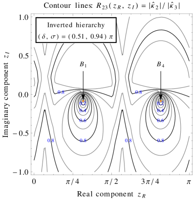
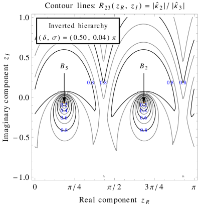
Fig. 1 illustrates that $R_{23}$ is periodic in the real component of $z$ with a period of $\pi/2$,

$$R_{23}\left(\delta,\sigma;z\right)=R_{23}\left(\delta,\sigma;z+n\,\frac{\pi}{2}\right)\,,\quad n\in\mathbb{Z}\,.$$ (25)

This can be understood by noting that a shift of $z$ by an amount $\pi/2$ along the real axis basically corresponds to nothing but a column exchange in the Yukawa matrix $\kappa_{\alpha I}$ (see Eq. (12)),

$$z\rightarrow z+\frac{\pi}{2}\quad\Rightarrow\quad\kappa_{\alpha 1}\rightarrow\kappa_{\alpha 2}\,,\quad\kappa_{\alpha 2}\rightarrow-\kappa_{\alpha 1}\,.$$ (26)

Up to possible sign changes, this transformation, therefore, leaves the list of sorted Yukawa couplings, $\hat{\kappa}$, unaffected, so that the value of $R_{23}$ remains the same. Similarly, it is worthwhile pointing out that $R_{23}$ as a function of $\delta$, $\sigma$, and $z$ is invariant under the following transformation,

$$\delta\rightarrow-\delta\,,\quad\sigma\rightarrow-\sigma\,,\quad z\rightarrow z^{*}\,,$$ (27)

which amounts to a complex conjugation of the Yukawa couplings $\kappa_{\alpha I}$ (see Eq. (12)). As the hierarchy parameter $R_{23}$ is defined in terms of the absolute values of the sorted Yukawa couplings, $R_{23}=\left|\hat{\kappa}_{2}\right|/\left|\hat{\kappa}_{3}\right|$, it remains unchanged under this transformation. An important consequence of this property of $R_{23}$ is that it essentially halves the domain of $R_{23}$ on the $\delta$ axis,

$$R_{23}\left(2\pi-\delta,\sigma;z\right)=R_{23}\left(\delta,\pi-\sigma;z^{*}\right)\,.$$ (28)

We note that it is this “reflection symmetry” of the parameter $R_{23}$ in the $\left(\delta,\sigma\right)$ plane, which is responsible for the fact that, in Eq. (19), we actually find two solutions for $\delta$ and $\sigma$ for both two-zero textures. In studying $R_{23}$ as a function of $\delta$, $\sigma$, and $z$, we, therefore, do not need to consider the full $\delta$ range, $\delta\in\left[0,2\pi\right)$, but can restrict ourselves to the restricted interval $\delta\in\left[0,\pi\right]$.

Figure 2: Minimized hierarchy parameter $H_{23}$ as a function of the $CP$-violating phases $\delta$ and $\sigma$ for normal (upper panel) and inverted neutrino mass ordering (lower panel), see Eq. (34). The contour lines represent the function values of $H_{23}$ in the $\left(\delta,\sigma\right)$ plane, while the color shading indicates the corresponding (approximate) Yukawa textures according to Eq. (15). The colored points mark the local minima of $H_{23}$, see also Tab. 2.

Finally, it is interesting to study $R_{23}$ in the limit of large $\left|\textrm{Im}\left\{z\right\}\right|$. Unlike the real component of $z$, the imaginary component of $z$ is not restricted to a periodic interval. $\left|\textrm{Im}\left\{z\right\}\right|$ can, therefore, take arbitrarily large values, which is the reason why the parameter space of our model is unbounded. Let us first consider the individual rescaled Yukawa couplings $\kappa_{\alpha I}$ in the limit of large $\left|\textrm{Im}\left\{z\right\}\right|$. Decomposing the complex parameter $z$ into its real and imaginary parts, $z=z_{R}+i\,z_{I}$, the Casas-Ibarra parametrization in Eq. (12) may be rewritten as follows,

$$\kappa_{\alpha 1} =\frac{1}{2}\left[\left(V_{\alpha k}+i\,V_{\alpha l}\right)e^{z_{I}-i\,z_{R}}+\left(V_{\alpha k}-i\,V_{\alpha l}\right)e^{-z_{I}+i\,z_{R}}\right]\,,$$ (29)

$$\kappa_{\alpha 2} =\frac{1}{2}\left[\left(V_{\alpha l}-i\,V_{\alpha k}\right)e^{z_{I}-i\,z_{R}}+\left(V_{\alpha l}+i\,V_{\alpha k}\right)e^{-z_{I}+i\,z_{R}}\right]\,,$$

where $\left(k,l\right)=\left(2,3\right)$ in the NH case and $\left(k,l\right)=\left(1,2\right)$ in the IH case. In the limit of large $\left|z_{I}\right|$, we can either neglect the terms proportional to $e^{z_{I}}$ or to $e^{-z_{I}}$, such that Eq. (29) simplifies to

$$z_{I}\gg 1 \quad\Rightarrow\quad\kappa_{\alpha 1}\simeq i\,\kappa_{\alpha 2}\simeq\frac{1}{2}\left(V_{\alpha k}+i\,V_{\alpha l}\right)e^{z_{I}-i\,z_{R}}\,,$$ (30)

$$z_{I}\ll-1 \quad\Rightarrow\quad\kappa_{\alpha 2}\simeq i\,\kappa_{\alpha 1}\simeq\frac{1}{2}\left(V_{\alpha l}+i\,V_{\alpha k}\right)e^{-z_{I}+i\,z_{R}}\,.$$

In either case, we find that the two columns in $\kappa_{\alpha I}$ become—up to a relative phase—equal to each other. For $\left|z_{I}\right|\gg 1$, the list of sorted couplings, $\hat{\kappa}$, consequently takes the following form,

$$\left|z_{I}\right|\gg 1 \quad\Rightarrow\quad\hat{\kappa}\simeq\left(\kappa_{\alpha_{1}1},\kappa_{\alpha_{1}2},\kappa_{\alpha_{2}1},\kappa_{\alpha_{2}2},\kappa_{\alpha_{3}1},\kappa_{\alpha_{3}2}\right)\,,$$ (31)

where the indices $\left(\alpha_{1},\alpha_{2},\alpha_{3}\right)$ represent the permutation of $\left(e,\mu,\tau\right)$ that satisfies the relation $\left|\kappa_{\alpha_{1}I}\right|\leq\left|\kappa_{\alpha_{2}I}\right|\leq\left|\kappa_{\alpha_{3}I}\right|$. Physically, such a Yukawa configuration corresponds to an (approximate) alignment in flavor space of the two linear combinations of lepton flavors that couple to $N_{1}$ and $N_{2}$, respectively. Without any additional physical assumption, e.g., an additional flavor symmetry at high energies, such an alignment, however, appears unnatural or fine-tuned. On top of that, too close an alignment results in a flavor structure that only manages to account for the low-energy data on neutrino masses and mixings by means of precise cancellations among rather large Yukawa couplings—which also appears unnatural. In the limit of exact flavor alignment, $\kappa_{\alpha 1}\equiv\kappa_{\alpha 2}$, it is even impossible to explain all of the low-energy data, because the number of available high-energy DOFs is simply too small. For these reasons, we will be more interested in values of $\left|z_{I}\right|$ of $\mathcal{O}(1)$ in the following. On the other hand, as we cannot exclude the possibility of aligned lepton flavors, we will, of course, keep our analysis as general as possible and also devote some attention to the case of large $\left|z_{I}\right|$ in our parameter scan.

An important implication of Eq. (30) for our purposes is that, in the regime of large $\left|z_{I}\right|$, ratios of Yukawa couplings no longer depend on $z$. This means that, for $z_{I}\rightarrow\pm\infty$, the hierarchy parameter $R_{23}$ is bound to asymptotically approach a constant value, $R_{23}^{+}$ and $R_{23}^{-}$, respectively,

$$z_{I}\rightarrow\pm\infty\quad\Rightarrow\quad R_{23}\rightarrow R_{23}^{\pm}=\left|\frac{V_{\alpha_{1}k}\pm i\,V_{\alpha_{1}l}}{V_{\alpha_{2}k}\pm i\,V_{\alpha_{2}l}}\right|\,.$$ (32)

In the case of the two scenarios shown in Fig. 1, we obtain, e.g., the following asymptotic values,

$$\left(R_{23}^{+},R_{23}^{-}\right)=\begin{cases}\left(0.81,0.68\right)&;\quad\left(\delta,\sigma\right)=\left(0.51,0.94\right)\pi\\ \left(0.61,0.89\right)&;\quad\left(\delta,\sigma\right)=\left(0.50,0.04\right)\pi\end{cases}\,,$$ (33)

which are all more or less close to $1$. This is to say that, in these two scenarios, we are not missing any strong hierarchy in the neutrino Yukawa matrix that could potentially be realized in regions of the complex $z$ plane that are not displayed in Fig. 1. Instead, the local minima depicted in Fig. 1 are really the only minima of $R_{23}$ there are in the complex $z$ plane.

4 Maximal Yukawa hierarchies in dependence of $\delta$ and $\sigma$

	$\left(\delta,\sigma\right)/\pi$	Texture	$H_{23}$	$z_{I}$	Rescaled Yukawa matrix $\kappa\times 10^{7}$
NH-1	$\left(0.55,0.96\right)$ $\left(1.45,0.04\right)$	A1	$0.11$	$\ll-1$	$\begin{pmatrix}0.41\,e^{1.02\,i\pi}&0.41\,e^{1.52\,i\pi}\\ 3.85\,e^{1.38\,i\pi}&3.85\,e^{1.88\,i\pi}\\ 3.90\,e^{1.60\,i\pi}&3.90\,e^{0.10\,i\pi}\end{pmatrix}f\left(z\right)$ $\bigg{(}_{\bigg{(}_{\big{(}}}^{\bigg{(}^{\big{(}}}$
NH-2	$\left(1.00,0.00\right)$	B1/B4	$0.13$	$\mathcal{O}(1)$	$\begin{pmatrix}-0.18&\phantom{-}1.42\,\phantom{i}\\ \phantom{-}3.83&-0.18\,\phantom{i}\\ \phantom{-}3.11&-2.73\,\phantom{i}\end{pmatrix}\phantom{f\left(z\right)}$ $\bigg{(}_{\bigg{(}_{\big{(}}}^{\bigg{(}^{\big{(}}}$
NH-3	$\left(0.01,0.00\right)$ $\left(1.99,0.00\right)$	B2/B5	$0.19$	$\mathcal{O}(1)$	$\begin{pmatrix}0.27\,e^{0.01\,i\pi}&1.41\,e^{0.01\,i\pi}\\ 2.76\,\phantom{e^{0.01\,i\pi}}&2.53\,\phantom{e^{0.01\,i\pi}}\\ 4.21\,\phantom{e^{0.01\,i\pi}}&0.27\,\phantom{e^{0.01\,i\pi}}\end{pmatrix}\phantom{f\left(z\right)}$ $\bigg{(}_{\bigg{(}_{\big{(}}}^{\bigg{(}^{\big{(}}}$
IH-1	$\left(0.00,0.50\right)$	A2	$0.12$	$\gg+1$	$\begin{pmatrix}\phantom{-}7.30&-7.30\,i\\ \phantom{-}0.22&-0.22\,i\\ -1.92&\phantom{-}1.92\,i\end{pmatrix}f\left(z\right)$ $\bigg{(}_{\bigg{(}_{\big{(}}}^{\bigg{(}^{\big{(}}}$
IH-2	$\left(1.00,0.50\right)$	A3	$0.26$	$\gg+1$	$\begin{pmatrix}\phantom{-}7.30&-7.30\,i\\ \phantom{-}1.87&-1.87\,i\\ -0.49&\phantom{-}0.49\,i\end{pmatrix}f\left(z\right)$ $\bigg{(}_{\bigg{(}_{\big{(}}}^{\bigg{(}^{\big{(}}}$
IH-3	$\left(0.51,0.94\right)$ $\left(1.49,0.06\right)$	B1/B4	$0.00$	$\mathcal{O}(1)$	$\begin{pmatrix}0&5.24\,e^{1.02\,i\pi}\\ 3.54\,e^{1.04\,i\pi}&0\\ 4.06\,e^{0.04\,i\pi}&1.19\,e^{0.53\,i\pi}\end{pmatrix}\phantom{f\left(z\right)}$ $\bigg{(}_{\bigg{(}_{\big{(}}}^{\bigg{(}^{\big{(}}}$
IH-4	$\left(0.50,0.04\right)$ $\left(1.50,0.96\right)$	B2/B5	$0.00$	$\mathcal{O}(1)$	$\begin{pmatrix}0&5.25\,e^{1.99\,i\pi}\\ 3.52\,e^{0.97\,i\pi}&1.04\,e^{1.49\,i\pi}\\ 4.05\,e^{1.97\,i\pi}&0\end{pmatrix}\phantom{f\left(z\right)}$ $\bigg{(}_{\bigg{(}_{\big{(}}}^{\bigg{(}^{\big{(}}}$
IH-5	$\left(0.89,0.78\right)$ $\left(1.11,0.22\right)$	C3/C6	$0.18$	$\mathcal{O}(1)$	$\begin{pmatrix}5.83\,e^{1.06\,i\pi}&3.42\,e^{0.55\,i\pi}\\ 0.62\,e^{0.95\,i\pi}&3.42\,e^{0.19\,i\pi}\\ 0.62\,e^{0.94\,i\pi}&3.42\,e^{1.14\,i\pi}\end{pmatrix}\phantom{f\left(z\right)}$ $\bigg{(}_{\bigg{(}_{\big{(}}}^{\bigg{(}^{\big{(}}}$

Table 2: Minima of the minimized hierarchy parameter $H_{23}$ in the $\left(\delta,\sigma\right)$ plane for normal and inverse light-neutrino mass ordering, respectively, see Eq. (34). Nomenclature for the (approximate) textures according to Eq. (15). Large values of $\left|z_{I}\right|$ correspond to flavor alignment in the neutrino Yukawa matrix $\kappa_{\alpha I}$, while $\mathcal{O}(1)$ values of $\left|z_{I}\right|$ do not imply any particular correlation among the two columns in $\kappa_{\alpha I}$, see Eq. (29). At large values of $\left|z_{I}\right|$, all Yukawa couplings scale with $f\left(z\right)=1/2\,\exp\left[\textrm{sgn}\left\{z_{I}\right\}\left(z_{I}-i\,z_{R}\right)\right]$, see Eq. (30).

Figure 3: Minimized hierarchy parameter $H_{23}$ as a function of the $CP$-violating phases $\delta$ and $\sigma$ for normal mass ordering, see Eq. (34). The upper panel displays the results of minimizing $R_{23}$ only over values of $\left|z_{I}\right|$ of $\mathcal{O}(1)$ (no flavor alignment), while in the lower panel, we plot the asymptotic value $\min\left\{R_{23}^{-},R_{23}^{+}\right\}$ at $\left|z_{I}\right|\gg 1$ (flavor alignment), see Eq. (32). Contour lines, color shading, colored points, and plot legends as in Fig. 2.

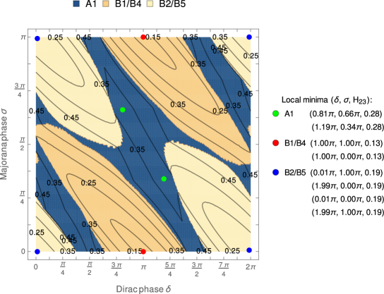
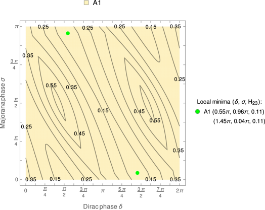
As explained in the previous section, an approximate [exact] two-zero texture in a given neutrino Yukawa matrix is characterized by a particularly small value [zero] of the hierarchy parameter $R_{23}\left(\delta,\sigma;z\right)$. For given values of the $CP$-violating phases $\delta$ and $\sigma$, we would, therefore, like to know how small a value $R_{23}$ can possibly take as a function of the rotation angle $z$. To answer this question, we are now going to study the minimized hierarchy parameter $H_{23}\left(\delta,\sigma\right)$,

$$H_{23}\left(\delta,\sigma\right)=\min_{z_{R}}\min_{z_{I}}R_{23}\left(\delta,\sigma;z\right)\,.$$ (34)

That is, for each pair of $\left(\delta,\sigma\right)$ values, we are going to minimize the ratio of sorted Yukawa couplings $R_{23}$ over the two real DOFs that are inaccessible at low energies in our model, $z_{R}$ and $z_{I}$. This eliminates the dependence of $R_{23}$ on the “unphysical” parameter $z$ and leaves us with a well-defined function in the $\left(\delta,\sigma\right)$ plane: At any given point in this plane, the function $H_{23}$ tells us how good a hierarchy in the neutrino Yukawa matrix one could, in principle, obtain. Without any extra assumptions, there is, of course, no reason why a certain value of $H_{23}$ should, indeed, be realized in Nature. It is always possible that, instead of the maximal Yukawa hierarchy for a particular pair of $\left(\delta,\sigma\right)$ values, only a weaker hierarchy is actually realized (which would then correspond to a point in the complex $z$ plane away from the global minimum of $R_{23}$). In this sense, our analysis will provide us with model-independent upper bounds on the quality of an approximate two-zero texture in dependence of $\delta$ and $\sigma$ that any UV completion has to satisfy. Here, note that a complete reconstruction of the entire neutrino Yukawa matrix from a measurement of $\delta$ and $\sigma$ is not feasible in our framework, anyway. The advantage of our approach, however, is that it will provide us with meaningful constraints on UV completions of the minimal seesaw model, no matter what the experimental outcome for $\delta$ and $\sigma$ will be.

It is straightforward to extend the philosophy behind our approach to other, more complicated neutrino mass models as well as to arbitrary textures. In the end, one always only has to follow the same three steps. (i) Express all high-energy Yukawa couplings in terms of two sets of parameters: low-energy observables on the one hand and “unphysical” parameters that are inaccessible at low energies on the other hand; (ii) define an appropriate ratio of (sorted) Yukawa couplings that is relevant to a certain texture; and (iii) marginalize this ratio over all unobservable parameters. This procedure should always results in phenomenological constraints on the Yukawa structures of interest in dependence of the available observables at low energies. Of course, the technical complexity of this algorithm grows with the number of inaccessible parameters. From this perspective, our analysis in this paper benefits from the fact that we are only dealing with two auxiliary parameters, $z_{R}$ and $z_{I}$. Or put differently: While our method appears to be applicable also in a more general context, we choose to illustrate our approach in the context of the minimal seesaw neutrino mass model because of its sheer simplicity.

A practical obstacle that one encounters when attempting to compute $H_{23}$ as a function of $\delta$ and $\sigma$ is that the hierarchy parameter $R_{23}$ is not a smooth function of the complex rotation angle $z$. Whenever the ordering among the sorted Yukawa couplings changes in consequence of a variation of $z$, $R_{23}$ experiences a “kink” at which it is longer differentiable. This observation leads us to forgo any further analytical calculations in the following. Instead, we shall search for the global minima of $R_{23}$ in the complex $z$ plane by means of a fully numerical analysis.

As discussed in Sec. 3, large values of $\left|z_{I}\right|$ lead to an alignment of the two columns in the neutrino Yukawa matrix, see Eq. (30). Physically, such a flavor alignment signals the presence of some kind of flavor symmetry at high energies, for which we do not have a proper justification from a low-energy perspective. On the other hand, we also cannot a priori exclude the possibility of flavor alignment. In the following, we are, therefore, going to explicitly distinguish between these two cases, i.e., between Yukawa matrices that do exhibit flavor alignment, $\left|z_{I}\right|\gg 1$, and those that do not, $\left|z_{I}\right|\sim\mathcal{O}(1)$. In this way, we will be able to track under which conditions certain textures arise and whether they rely on the assumption of flavor alignment or not.

Figure 4: Minimized hierarchy parameter $H_{23}$ as a function of the $CP$-violating phases $\delta$ and $\sigma$ for inverted mass ordering, see Eq. (34). The upper panel displays the results of minimizing $R_{23}$ only over values of $\left|z_{I}\right|$ of $\mathcal{O}(1)$ (no flavor alignment), while in the lower panel, we plot the asymptotic value $\min\left\{R_{23}^{-},R_{23}^{+}\right\}$ at $\left|z_{I}\right|\gg 1$ (flavor alignment), see Eq. (32). Contour lines, color shading, colored points, and plot legends as in Fig. 2.

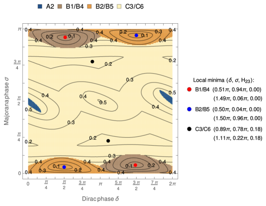
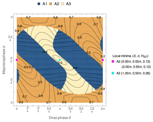
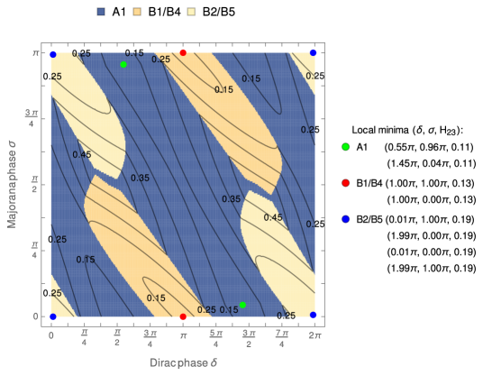
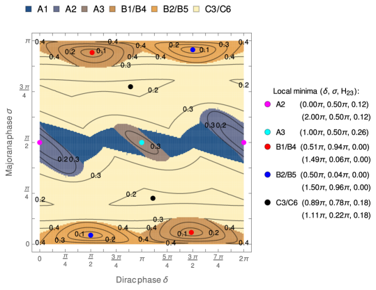
The outcome of our numerical scan is shown in Figs. 2, 3, 4, and 5. In Fig. 2, we present our results for $H_{23}$ as a function of $\delta$ and $\sigma$ after minimizing $R_{23}$ over the entire complex $z$ plane. The two panels of Fig. 2 correspond to NH and IH, respectively. Figs. 3 and 4 illustrate how these results decompose into contributions from “flavor-aligned” ($\left|z_{I}\right|\gg 1$) and “flavor-nonaligned” Yukawa matrices ($\left|z_{I}\right|\sim\mathcal{O}(1)$). Here, Fig. 3 summarizes our results for NH, while Fig. 4 summarizes our results for IH. The upper panels of Figs. 3 and 4 show our respective results for $H_{23}$ after minimizing $R_{23}$ over $z$ values not far from the real axis, $\left|z_{I}\right|\sim\mathcal{O}(1)$, whereas in the lower panels of Figs. 3 and 4, we plot the respective minimum of the two asymptotic values at large $\left|z_{I}\right|$, $\min\left\{R_{23}^{-},R_{23}^{+}\right\}$, see Eq. (32). In Fig. 5, we finally present a close-up of our results for $H_{23}$ in the vicinity of its exact zeros in the case of an inverted mass ordering. A summary of all local minima of the function $H_{23}$ in the $\left(\delta,\sigma\right)$ plane is given in Tab. 2.

Let us now comment on our numerical findings in more detail: As shown in Refs. [13, 24], the only exact two-zero textures that can be realized in the type-I seesaw model with two right-handed neutrinos are textures $B_{1,4}$ and $B_{2,5}$, and that only if one assumes an inverted hierarchy. In our scan, we readily recover these two exact textures as zeros of $H_{23}$ in the $\left(\delta,\sigma\right)$ plane. But in addition to that, our analysis has more to offer! The conventional top-down approach merely leads to precise predictions for $\delta$ and $\sigma$ under the assumption of exact texture zeros. If these predictions should turn out to be inconsistent with the experimental data at some point (which is maybe not unlikely), exact two-zero textures would be ruled out and the scenarios in Refs. [13, 24] would need to be declared unviable. In such a case, our analysis now shows how the assumption of exact texture zeros would need to be relaxed, so as still accommodate the experimental data. Fig. 5 indicates how strong a hierarchy in the neutrino Yukawa matrix we would at least have to assume, once $\delta$ and $\sigma$ should be measured at values that are slightly off the exact predictions in Eq. (19). Shifts in the values of $\delta$ and $\sigma$ by, say, $0.1\,\pi$ compared to the predictions in Eq. (19) would, e.g., require $\mathcal{O}\left(10\,\%\right)$ corrections to an exact two-zero texture. This generalization of the predictions in Eq. (19) is one of our main results in this paper. Our findings in Fig. 5 correspond to the theoretical error bars belonging to the “central values” in Eq. (19). In this sense, our study represents a crucial supplement to the analyses in Refs. [13, 24], which derive rather uncompromising predictions for specific and rigid theoretical assumptions.

Moreover, we find that, in addition to $B_{1,4}$ and $B_{2,5}$ textures, several other textures may be approximately realized in our neutrino mass model. In the NH case, we encounter matrices that belong to Yukawa structures $A_{1}$, $B_{1,4}$, and $B_{2,5}$; while in the IH case, we obtain structures of type $A_{1}$, $A_{2}$, $A_{3}$, $B_{1,4}$, $B_{2,5}$, and $C_{3,6}$. In certain regions in the $\left(\delta,\sigma\right)$ plane, i.e., in the vicinity of the local minima of $H_{23}$, these structures partially exhibit strong hierarchies, so that they may be regarded as approximate textures in the actual sense, see Tab. 2. Here, an interesting observation is that, also in the case of a normal mass ordering, the neutrino Yukawa matrix may exhibit a strong hierarchy. In the case of flavor alignment, we find, e.g., that at $\left(\delta,\sigma\right)\simeq\left(0.55,0.96\right)\pi$ as well as at $\left(\delta,\sigma\right)\simeq\left(1.45,0.04\right)\pi$ an approximate $A_{1}$ texture can be realized, with the smallest two entries in the neutrino Yukawa matrix being suppressed compared to the next-largest entry by roughly a factor of $10$. As soon as we relax the assumption of two exact texture zeros, the case of a normal mass hierarchy can, therefore, no longer be excluded. For sure, the type-I seesaw model with two right-handed neutrinos is still inconsistent with the assumption of an exact two-zero texture. This conclusion does not change. But a main result of our analysis is that also the NH case becomes feasible again, once we allow for small perturbations of $\mathcal{O}\left(10\,\%\right)$.

Figure 5: Minimized hierarchy parameter $H_{23}$ as a function of $\delta$ and $\sigma$ in the vicinity of its exact zeros (in the case of an inverted mass ordering), see Eq. (19). For both possible two-zero textures, $B_{1,4}$ and $B_{2,5}$, we respectively find two zeros in the $\left(\delta,\sigma\right)$ plane, which are related to each other via the reflection symmetry in Eq. (28).

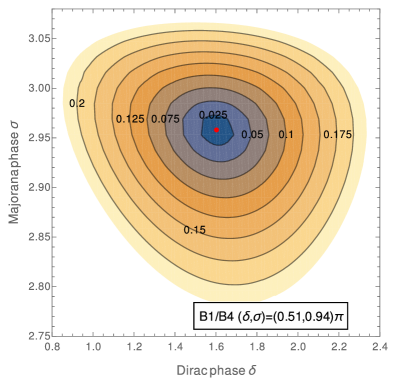
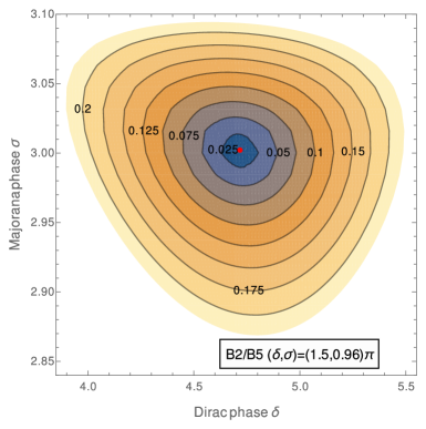
Another interesting observation is that the minimized hierarchy parameter $H_{23}$ turns out to have a preference for small function values close to points in the $\left(\delta,\sigma\right)$ plane that conserve $CP$ in the leptonic weak charged-current interactions (see the discussion in Ref. [1] for more details),

$$\frac{\left(\delta,\sigma\right)}{\pi}=\left(m,\frac{n}{2}\right)\,,\quad m,n\in\mathbb{Z}\quad\Rightarrow\quad\textrm{No $CP$ violation}\,.$$ (35)

This means that, out of the six “new” local minima of $H_{23}$ that we find in our analysis (NH-1, NH-2, NH-3, IH-1, IH-2, IH-5), three minima (NH-2, IH-1, IH-2) correspond to no $CP$ violation at all; in one minimum (NH-3), there is barely no $CP$ violation; and only two “new” minima (NH-1, IH-5) feature a sizable amount of $CP$ violation, see Tab. 2. If the recent experimental hints for a “maximal” $CP$-violating phase $\delta$ should be confirmed in upcoming experiments, the $CP$-conserving scenarios NH-2, NH-3, IH-1, and IH-2 would, therefore, need to be abandoned.

Last but not least, we comment on the interplay of “flavor-aligned” and “flavor-nonaligned” regions in Fig. 2. In the NH case, the effect of extending our search to large values of $\left|z_{I}\right|$ is that it (i) shrinks the region occupied by $B_{1,4}$ and $B_{2,5}$ textures and (ii) shifts (as well as deepens) the position of the local $A_{1}$ minima, see Fig. 3. In the IH case, “flavor-aligned” matrices are responsible for the horizontal band of $A_{1}$, $A_{2}$, and $A_{3}$ structures at $\sigma\sim\frac{\pi}{2}$. Here, regions, in which the structures $A_{2}$ and $A_{3}$ appear, exhibit local maxima in the nonaligned case, see Fig. 4.

5 Stability under variations of the experimental input data

In our numerical scan presented in Sec. 4, we always employ the best-fit values for all known experimental input values, see Tab. 1. Our numerical results are, thus, subject to small variations in case the “true” values for the light-neutrino masses and mixing angles should eventually be found to slightly deviate from the current best-fit values. To get a feeling for this dependence of our results on the experimental data, we are going to perform a naive $\chi^{2}$ analysis in the following. In doing so, we will neglect the detailed likelihood functions in Ref. [31] and simply treat all observables as if they were Gaussian. It is then straightforward to define $\chi^{2}$,

$$\chi^{2}\left(\left\{\mathcal{O}_{i}\right\}\right)=\sum_{i=1}^{5}\frac{\left(\mathcal{O}_{i}-\mathcal{O}_{i}^{\rm exp}\right)^{2}}{\left(\Delta\mathcal{O}_{i}^{\rm exp}\right)^{2}}\,,\quad\left\{\mathcal{O}_{i}\right\}=\left\{\delta m^{2},\Delta m^{2},\sin^{2}\theta_{12},\sin^{2}\theta_{13},\sin^{2}\theta_{23}\right\}\,.$$ (36)

Here, $\mathcal{O}_{i}^{\rm exp}$ stands for the respective best-fit values and $\Delta\mathcal{O}_{i}^{\rm exp}$ for the respective widths of the full $\pm 3\,\sigma$ ranges divided by six, see Tab. 1. For each choice of values for the five experimental input observables, $\left\{\mathcal{O}_{i}\right\}$, Eq. (36) provides us with a $\chi^{2}$ value that we can use as a likelihood measure. Under the assumption of Gaussian distributions and given the fact that we are working with, in total, five independent degrees of freedom, $\chi^{2}$ values of $\chi^{2}=\left(5,89,11.31,18.21\right)$ correspond to deviations from the global best-fit configuration at the $\left(1\sigma,2\sigma,3\sigma\right)$ confidence level, respectively.

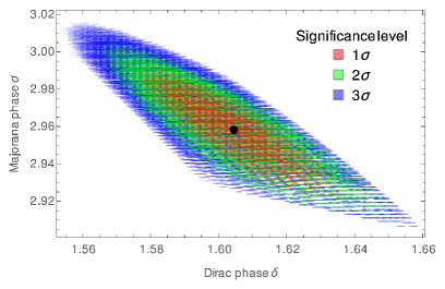
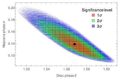
To give an example of how varying the experimental input data affects our results, we are now going to study the stability of the predictions in Eq. (19). We proceed in three steps: (i) First of all, we vary all five observables within their experimental $\pm 3\,\sigma$ ranges; (ii) for each set of input values, we then determine the predictions for $\delta$ and $\sigma$ according to Eq. (14), assuming either an exact $B_{1,4}$ or an exact $B_{2,5}$ texture; and (iii) finally, we associate these predictions with the corresponding value of $\chi^{2}$, calculated according to Eq. (36). This procedure yields $\chi^{2}$ as a function of $\delta$ and $\sigma$, for both an exact $B_{1,4}$ and an exact $B_{2,5}$ texture, which can, in turn, be translated into $1\,\sigma$, $2\,\sigma$, and $3\,\sigma$ confidence intervals in the $\left(\delta,\sigma\right)$ plane. The outcome of this analysis is shown in Fig. 6. As evident from this figure, the experimental uncertainty in the neutrino observables induces shifts in $\delta$ and $\sigma$ at the level of $\mathcal{O}\left(1\,\%\right)\pi$—and is, hence, nearly negligible. The requirement of exact texture zeros in the Yukawa matrix in combination with the current experimental errors determines $\delta$ and $\sigma$ to high precision. This leads us to conclude that all of our results in Sec. 4 ought to be stable under the variation of the input data within the current experimental limits. Any further quantitative statement beyond this qualitative conclusion would require a more sophisticated analysis, which is beyond the scope of this work.

Figure 6: Stability of the predictions for $\left(\delta,\sigma\right)$ under variation of the experimental input parameters $\delta m^{2}$, $\Delta m^{2}$, $\sin^{2}\theta_{12}$, $\sin^{2}\theta_{13}$, and $\sin^{2}\theta_{23}$ for an exact $B_{1,4}$ texture (left panel) and an exact $B_{2,5}$ texture (right panel). The black dots mark the predictions for $\left(\delta,\sigma\right)$ if all observables are set to their best-fit values, $\left(\delta,\sigma\right)=\left(0.51,0.94\right)\pi$ in the $B_{1,4}$ case and $\left(\delta,\sigma\right)=\left(0.50,0.04\right)\pi$ in the $B_{2,5}$ case, see Eq. (19). $\chi^{2}$ is calculated according to Eq. (36).

6 Conclusions

The type-I seesaw mechanism with only two right-handed neutrinos is a minimal neutrino mass model that manages to account for all observed mass-squared differences and mixing angles in the SM neutrino sector. Compared to the conventional three-right-handed-neutrino scenario, the minimal seesaw model comes with a smaller number of parameters that are inaccessible at low energies and is, thus, more predictive. In addition, it complies with the philosophy of Occam’s razor, which calls on us to always only make as few assumptions as necessary.

Figure 7: Complementarity between conventional model building and our approach in this paper. Top-down model building (right to left) typically makes non-injective predictions for the outcome of experimental measurements. Depending on the specific assumptions made when building UV flavor models, one may not have a fitting model at hand for each conceivable experimental result. Meanwhile, it is clear that the list of flavor models in the literature is not exhaustive and that there are still many models that await to be worked out. In our bottom-up approach (left to right), we remain, by contrast, agnostic as to what UV dynamics are exactly responsible for the form of the neutrino Yukawa matrix. By scanning the entire complex $z$ plane, we make sure to cover all UV completions of the minimal seesaw model, independently of whether each of these models (i.e., each of these points in the $z$ plane) has already been recognized as a particularly well motivated flavor structure or not. This provides us with a function, $H_{23}$, defined on the entire domain of conceivable experimental data (see Eq. (34)). No matter what values for $\delta$ and $\sigma$ future experiments will find, once we interpret the new data in the context of the minimal seesaw model, we will always learn something new about the underlying flavor structure at high energies.

In the context of this model, we have addressed the following question is this paper: Suppose leptonic $CP$ violation should be conclusively measured in the near future, what lessons could we possibly learn from such a measurement about the underlying Yukawa structure of the SM neutrino sector? In particular, we were interested in studying to what extent one would still be able to realize (approximate) textures zeros in the neutrino Yukawa matrix for given values of the $CP$-violating phases $\delta$ and $\sigma$. In order to answer this question, we introduced a novel hierarchy parameter, $R_{23}$ (see Eq. (22)), in terms of a ratio of ordered Yukawa couplings. Minimizing this hierarchy parameter over all “unphysical” parameters (i.e., all parameters that are inaccessible at low energies), we were then able to identify the respective maximal Yukawa hierarchies for each pair of hypothetical $\left(\delta,\sigma\right)$ values. This analysis led us to several interesting results:

• We recovered the exact two-zero textures $B_{1,4}$ and $B_{2,5}$ that can be realized in the IH case, see Figs. 2 and 4. In addition, we were able to quantify to what an extent the assumption of exact texture zeros would need to be relaxed, if the phases $\delta$ and $\sigma$ should eventually be measured at values slightly off the expected values in these two scenarios, see Fig. 5. Besides that, we stress on a more theoretical note that one can imagine many possibilities how, in the ultimate theory of flavor, texture zeros may end up being disturbed (e.g., via quantum or gravitational effects). Against this backdrop, our results in Fig. 5 should be regarded as the theoretical error bars belonging to the precise predictions in Eq. (19).

• We found that, allowing for perturbations of $\mathcal{O}\left(10\,\%\right)$, approximate two-zero textures may also be realized in the NH case; e.g., an approximate $A_{1}$ texture at $\left(\delta,\sigma\right)=\left(0.55,0.96\right)\pi$ or at $\left(\delta,\sigma\right)=\left(1.45,0.04\right)\pi$, see Figs. 2 and 3. This conclusion represents an important caveat to the conventional wisdom that the type-I seesaw mechanism involving only two right-handed neutrinos actually does not allow for two-zero textures in the NH case.

• We observed that the minimized hierarchy parameter $H_{23}$ (see Eq. (34)) tends to take particularly small values at $\left(\delta,\sigma\right)$ values that conserve $CP$. Our list of approximate two-zero textures in Tab. 2, therefore, splits into $CP$-preserving as well as $CP$-violating scenarios.

• We studied the interplay of “flavor-aligned” and “flavor-nonaligned” Yukawa matrices, see Figs. 3 and 4, arriving at the conclusion that the possibility of flavor alignment should not be neglected when searching for the global minima of the hierarchy parameter $R_{23}$.

• Finally, we checked the stability of our numerical results under variations of the experimental input data. We found that the experimental uncertainties in the low-energy observables shift our predictions for $\delta$ and $\sigma$ at the level of $\mathcal{O}\left(1\,\%\right)\pi$, see Fig. 6. This is safely negligible.

In closing, we emphasize that we performed a data-driven bottom-up analysis, see Fig. 7. Instead of starting from the high-energy perspective (i.e., choosing a particular UV flavor model and calculating the corresponding predictions for the low-energy observables), we based our analysis on the question as to what might be seen in neutrino experiments in the near future. This is a complementary approach, which allows to derive data-driven and model-independent constraints on all conceivable UV completions of the minimal seesaw model, irrespectively of whether these models can already be found in the literature or still need to be discovered.

Of course, all of our results heavily rely on the assumption of only two right-handed neutrinos and should only be interpreted in this context. If experiments should find that the lightest neutrino mass eigenstate has nonzero mass, $\textrm{min}\left\{m_{i}\right\}>0$, our numerical results would become obsolete. Our general strategy, on the other hand, appears to be useful also in the context of other models and with regard to other types of Yukawa structures. In the usual seesaw model with three right-handed neutrinos, one might, e.g., introduce a hierarchy parameter $R_{mn}=\left|\hat{\kappa}_{m}\right|/\left|\hat{\kappa}_{n}\right|$ as a measure for the gap between the $m^{\rm th}$ and the $n^{\rm th}$ entry in the list of ordered Yukawa couplings $\hat{\kappa}$ (see also Eq. (22)). Minimizing this parameter over the three complex phases in the Casas-Ibarra parametrization of the three-neutrino Yukawa matrix, $\omega_{12}$, $\omega_{13}$, and $\omega_{23}$,

$$H_{mn}\left(\delta,\sigma\right)=\min_{\omega_{12}}\min_{\omega_{13}}\min_{\omega_{23}}R_{mn}\left(\delta,\sigma;\omega_{12},\omega_{13},\omega_{23}\right)\,,$$ (37)

would then allow to study arbitrary textures in a very general context. Of course, the technical complexity of such an analysis would increase with the number of undetermined parameters. But we believe that, in principle, our method should be applicable in a broad class of models and for a large variety of Yukawa structures. In the end, extending our analysis to other neutrino mass models would serve as an important preparation for the anticipated data on $CP$ violation in the lepton sector. Only if top-down model building and bottom-up data analysis go hand in hand, we will be able to make progress in our understanding of the SM flavor structure.

Acknowledgements

T. R. would like to thank Moritz Platscher for helpful discussions. K. S. would like to thank Tsutomu T. Yanagida for inspiring comments at the early stages of this project.

References

- [1] K. A. Olive et al. [Particle Data Group Collaboration], Review of Particle Physics, Chin. Phys. C 38, 090001 (2014).
- [2] N. Cabibbo, Time Reversal Violation in Neutrino Oscillation, Phys. Lett. B 72, 333 (1978); for a review, see: G. C. Branco, R. G. Felipe and F. R. Joaquim, Leptonic CP Violation, Rev. Mod. Phys. 84, 515 (2012), arXiv:1111.5332 [hep-ph].
- [3] B. Pontecorvo, Inverse beta processes and nonconservation of lepton charge, Sov. Phys. JETP 7, 172 (1958), Zh. Eksp. Teor. Fiz. 34, 247 (1957); Z. Maki, M. Nakagawa and S. Sakata, Remarks on the unified model of elementary particles, Prog. Theor. Phys. 28, 870 (1962).
- [4] D. S. Ayres et al. [NOA Collaboration], NOA: Proposal to build a 30 kiloton off-axis detector to study oscillations in the NuMI beamline, hep-ex/0503053.
- [5] K. Abe et al. [T2K Collaboration], Indication of Electron Neutrino Appearance from an Accelerator-produced Off-axis Muon Neutrino Beam, Phys. Rev. Lett. 107, 041801 (2011), arXiv:1106.2822 [hep-ex].
- [6] P. Vahle [NOA Collaboration], New Results from NOA, presented at the “XXVII International Conference on Neutrino Physics and Astrophysics (Neutrino 2016)”, London, United Kingdom, July 4–9, 2016, NOVA-doc-15688-v15.
- [7] R. Acciarri et al. [DUNE Collaboration], Long-Baseline Neutrino Facility (LBNF) and Deep Underground Neutrino Experiment (DUNE): Volume 2: The Physics Program for DUNE at LBNF, arXiv:1512.06148 [physics.ins-det].
- [8] T. Yanagida, Horizontal Symmetry And Masses Of Neutrinos, in “Proceedings of the Workshop on the Unified Theory and the Baryon Number in the Universe”, Tsukuba, Japan, February 13–14, 1979, edited by O. Sawada and A. Sugamoto, KEK report KEK-79-18, Conf. Proc. C 7902131, 95 (1979); Prog. Theor. Phys. 64, 1103 (1980); M. Gell-Mann, P. Ramond and R. Slansky, Complex Spinors and Unified Theories, in “Supergravity”, North-Holland, Amsterdam (1979), edited by D. Z. Freedom and P. van Nieuwenhuizen, CERN report Print-80-0576, Conf. Proc. C 790927, 315 (1979), arXiv:1306.4669 [hep-th]; see also: P. Minkowski, at a Rate of One Out of Muon Decays?, Phys. Lett. B 67, 421 (1977).
- [9] M. Fukugita and T. Yanagida, Baryogenesis Without Grand Unification, Phys. Lett. B 174, 45 (1986).
- [10] For reviews, see: G. Altarelli and F. Feruglio, Discrete Flavor Symmetries and Models of Neutrino Mixing, Rev. Mod. Phys. 82, 2701 (2010), arXiv:1002.0211 [hep-ph]; S. F. King and C. Luhn, Neutrino Mass and Mixing with Discrete Symmetry, Rept. Prog. Phys. 76, 056201 (2013), arXiv:1301.1340 [hep-ph].
- [11] S. F. King, Atmospheric and solar neutrinos with a heavy singlet, Phys. Lett. B 439, 350 (1998), hep-ph/9806440; Atmospheric and solar neutrinos from single right-handed neutrino dominance and family symmetry, Nucl. Phys. B 562, 57 (1999), hep-ph/9904210; Large mixing angle MSW and atmospheric neutrinos from single right-handed neutrino dominance and family symmetry, Nucl. Phys. B 576, 85 (2000), hep-ph/9912492.
- [12] P. H. Frampton, S. L. Glashow and T. Yanagida, Cosmological sign of neutrino CP violation, Phys. Lett. B 548, 119 (2002), hep-ph/0208157.
- [13] K. Harigaya, M. Ibe and T. T. Yanagida, Seesaw Mechanism with Occam’s Razor, Phys. Rev. D 86, 013002 (2012), arXiv:1205.2198 [hep-ph].
- [14] T. Endoh, S. Kaneko, S. K. Kang, T. Morozumi and M. Tanimoto, CP violation in neutrino oscillation and leptogenesis, Phys. Rev. Lett. 89, 231601 (2002), hep-ph/0209020.
- [15] A. D. Sakharov, Violation of Invariance, Asymmetry, and Baryon Asymmetry of the Universe, Pisma Zh. Eksp. Teor. Fiz. 5, 32 (1967), JETP Lett. 5, 24 (1967), Sov. Phys. Usp. 34, 392 (1991), Usp. Fiz. Nauk 161, 61 (1991).
- [16] G. Bambhaniya, P. S. B. Dev, S. Goswami, S. Khan and W. Rodejohann, Naturalness, Vacuum Stability and Leptogenesis in the Minimal Seesaw Model, arXiv:1611.03827 [hep-ph].
- [17] M. Flanz, E. A. Paschos, U. Sarkar and J. Weiss, Baryogenesis through mixing of heavy Majorana neutrinos, Phys. Lett. B 389, 693 (1996), hep-ph/9607310; A. Pilaftsis, violation and baryogenesis due to heavy Majorana neutrinos, Phys. Rev. D 56, 5431 (1997), hep-ph/9707235; A. Pilaftsis and T. E. J. Underwood, Resonant leptogenesis, Nucl. Phys. B 692, 303 (2004), hep-ph/0309342.
- [18] F. Björkeroth, S. F. King, K. Schmitz and T. T. Yanagida, Leptogenesis after Chaotic Sneutrino Inflation and the Supersymmetry Breaking Scale, arXiv:1608.04911 [hep-ph].
- [19] M. Kobayashi and T. Maskawa, Violation in the Renormalizable Theory of Weak Interaction, Prog. Theor. Phys. 49, 652 (1973).
- [20] M. Agostini et al. [GERDA Collaboration], Results on Neutrinoless Double- Decay of 76Ge from Phase I of the GERDA Experiment, Phys. Rev. Lett. 111, 122503 (2013), arXiv:1307.4720 [nucl-ex].
- [21] A. Osipowicz et al. [KATRIN Collaboration], KATRIN: A Next generation tritium beta decay experiment with sub-eV sensitivity for the electron neutrino mass. Letter of intent, hep-ex/0109033.
- [22] M. Raidal and A. Strumia, Predictions of the most minimal seesaw model, Phys. Lett. B 553, 72 (2003), hep-ph/0210021; A. Ibarra and G. G. Ross, Neutrino phenomenology: The Case of two right-handed neutrinos, Phys. Lett. B 591, 285 (2004), hep-ph/0312138.
- [23] S. F. King, Minimal predictive see-saw model with normal neutrino mass hierarchy, JHEP 1307, 137 (2013), arXiv:1304.6264 [hep-ph].
- [24] J. Zhang and S. Zhou, A Further Study of the Frampton-Glashow-Yanagida Model for Neutrino Masses, Flavor Mixing and Baryon Number Asymmetry, JHEP 1509, 065 (2015), arXiv:1505.04858 [hep-ph].
- [25] S. Weinberg, The Problem of Mass, Trans. New York Acad. Sci. 38, 185 (1977).
- [26] S. Antusch and O. Fischer, Non-unitarity of the leptonic mixing matrix: Present bounds and future sensitivities, JHEP 1410, 094 (2014), arXiv:1407.6607 [hep-ph]; Testing sterile neutrino extensions of the Standard Model at future lepton colliders, JHEP 1505, 053 (2015), arXiv:1502.05915 [hep-ph].
- [27] J. A. Casas and A. Ibarra, Oscillating neutrinos and , Nucl. Phys. B 618, 171 (2001), hep-ph/0103065.
- [28] S. F. King, Predicting neutrino parameters from family symmetry and quark-lepton unification, JHEP 0508, 105 (2005), hep-ph/0506297.
- [29] F. Björkeroth, F. J. de Anda, I. de Medeiros Varzielas and S. F. King, Leptogenesis in minimal predictive seesaw models, JHEP 1510, 104 (2015), arXiv:1505.05504 [hep-ph].
- [30] D. V. Forero, M. Tortola and J. W. F. Valle, Neutrino oscillations refitted, Phys. Rev. D 90, 093006 (2014), arXiv:1405.7540 [hep-ph]; M. C. Gonzalez-Garcia, M. Maltoni and T. Schwetz, Global Analyses of Neutrino Oscillation Experiments, Nucl. Phys. B 908, 199 (2016), arXiv:1512.06856 [hep-ph].
- [31] F. Capozzi, E. Lisi, A. Marrone, D. Montanino and A. Palazzo, Neutrino masses and mixings: Status of known and unknown parameters, Nucl. Phys. B 908, 218 (2016), arXiv:1601.07777 [hep-ph].
- [32] T. Banks and N. Seiberg, Symmetries and Strings in Field Theory and Gravity, Phys. Rev. D 83, 084019 (2011), arXiv:1011.5120 [hep-th].
- [33] T. Rink, K. Schmitz and T. T. Yanagida, Minimal Seesaw Model with a Discrete Heavy-Neutrino Exchange Symmetry, arXiv:1612.08878 [hep-ph].
- [34] C. D. Froggatt and H. B. Nielsen, Hierarchy of Quark Masses, Cabibbo Angles and CP Violation, Nucl. Phys. B 147, 277 (1979).