Nonuniform dependence on initial data for compressible gas dynamics: The periodic Cauchy problem

Barbara L. Keyfitz and Feride TฤฑฤŸlay
Abstract

We start with the classic result that the Cauchy problem for ideal compressible gas dynamics is locally well posed in time in the sense of Hadamard; there is a unique solution that depends continuously on initial data in Sobolev space Hssuperscript๐ป๐‘ H^{s} for s>d/2+1๐‘ ๐‘‘21s>d/2+1 where $d$ is the space dimension. We prove that the data to solution map for periodic data in two dimensions although continuous is not uniformly continuous on any bounded subset of Sobolev class functions.

The compressible gas dynamics equations of ideal hydrodynamics are given by the system

$$\begin{split}\rho_{t}+\nabla\cdot(\rho{\bf u})&=0\\ (\rho{\bf u})_{t}+\nabla\left(\rho{\bf u}\times{\bf u}\right)+\nabla p&=0\\ (E\rho)_{t}+\nabla\cdot\left(E\rho{\bf u}+p{\bf u}\right)&=0\end{split}$$ (1)

with ${\displaystyle E=e+\frac{1}{2}|{\bf u}|^{2}}$ the total energy and ${\displaystyle e=\frac{p}{(\gamma-1)\rho}}$ the internal energy, expressed in terms of density $\rho$, pressure $p$ and velocity $\bf u$.

Classical solutions and well-posedness in Sobolev spaces (existence and uniqueness of solutions as well as continuous dependence of solutions on initial data) of the initial value problem for (1) have been studied extensively, see for instance [9], [14], [15] and [17]. Sobolev space results are all local in time. In one space dimension shock waves form in finite time for almost all data in Hssuperscript๐ป๐‘ H^{s}, and for later times only weak solutions exist. (The definition of weak solutions, and well-posedness theory in $BV_{\textrm{loc}}\cap L^{1}_{\textrm{loc}}$, which are not the subject of this paper, can be found in [2] and [3].) In higher dimensions there is as yet no existence theory for weak solutions, and classical (Sobolev space) solutions have a finite-time life span for almost all data [14, 17].

Our goal is to study continuity properties of the solution map for classical solutions; in this paper we prove that for periodic data the initial-data to solution map is not uniformly continuous in Sobolev spaces. In a companion paper, [8], we extend this result to Hssuperscript๐ป๐‘ H^{s} data in the plane. Throughout, we assume s๐‘ s to be large enough for classical results to hold.

We consider solutions $U=U({\bf x},t)$ that take values in a compact subset of the state space $G=\{U\equiv(\rho,{\bf u},p)\mid\rho,p>0\}$, defined as the region where the physical quantities $\rho$ and $e$ are positive, and the system is symmetrizable hyperbolic.

In two dimensions, since we are considering classical solutions, we can ignore conservation form and write system (1) as

$$\begin{split}\rho_{t}+u\rho_{x}+v\rho_{y}+\rho(u_{x}+v_{y})&=0\\ u_{t}+uu_{x}+vu_{y}+h_{x}+\frac{h}{\rho}\rho_{x}&=0\\ v_{t}+uv_{x}+vv_{y}+h_{y}+\frac{h}{\rho}\rho_{y}&=0\\ h_{t}+uh_{x}+vh_{y}+(\gamma-1)h(u_{x}+v_{y})&=0\,.\end{split}$$ (2)

The parameter $\gamma$ denotes the ratio of specific heats (typically $1<\gamma<3$) and $h=p/\rho=(\gamma-1)e$ is a multiple of the internal energy.

We study this system in Sobolev spaces on the two dimensional torus: Hsโ€‹(๐•‹2)superscript๐ป๐‘ superscript๐•‹2H^{s}(\mathbb{T}^{2}) where $\mathbb{T}=\mathbb{R}/2\pi\mathbb{Z}$. The Sobolev norm is given by

โ€–uโ€–s2=โŸจฮ›sโ€‹u,ฮ›sโ€‹uโŸฉ,superscriptsubscriptnorm๐‘ข๐‘ 2superscriptฮ›๐‘ ๐‘ขsuperscriptฮ›๐‘ ๐‘ข\|u\|_{s}^{2}=\langle\Lambda^{s}u,\Lambda^{s}u\rangle\,,

where ฮ›s=(1โˆ’ฮ”)s/2superscriptฮ›๐‘ superscript1ฮ”๐‘ 2\Lambda^{s}=(1-\Delta)^{s/2} and $\langle\ ,\ \rangle$ denotes the $L^{2}$ inner product. Defining $U=(\rho,u,v,h)$ and $U(t)=U(\cdot,t)$, our main result is

Theorem 1 (Nonuniform Dependence on Initial Data)

For s>2๐‘ 2s>2, the data to solution map $U(0)\to U(t)$ for the system (2) is not uniformly continuous from any bounded subset of (Hsโ€‹(๐•‹2))4superscriptsuperscript๐ป๐‘ superscript๐•‹24(H^{s}(\mathbb{T}^{2}))^{4} into Cโ€‹([0,T];(Hsโ€‹(๐•‹2))4)๐ถ0๐‘‡superscriptsuperscript๐ป๐‘ superscript๐•‹24C([0,T];(H^{s}(\mathbb{T}^{2}))^{4}).

We note the significance of s>2๐‘ 2s>2. The well-posedness theory for symmetrizable hyperbolic systems, which forms the basis for our analysis, is credited to Gรฅrding [4], Leray [12], Kato [9] and Lax [11]. Solutions for quasilinear systems in $d$ space dimensions exist in spaces Hssuperscript๐ป๐‘ H^{s} for s>d/2+1๐‘ ๐‘‘21s>d/2+1. Modern expositions of the theory can be found in Majda [13], Serre [15] or Taylor [16].

We give the proof of Theorem 1 in Section 3. Our proof uses a framework introduced to prove an analogous result for the incompressible Euler equations of ideal hydrodynamics in [7]. This framework has been used for other nonlinear PDE including the Benjamin-Ono equation in [10] and the Camassa-Holm equation on the real line and on the one dimensional torus in [5] and [6] respectively. Implementation of this framework for the periodic Cauchy problem for the incompressible two-dimensional Euler equations is carried out in [7] with minimal technicalities. In that case, two sequences of exact solutions $\{U_{-1,n}(t)\}$ and $\{U_{1,n}(t)\}$ in Hssuperscript๐ป๐‘ H^{s} are constructed such that as $n\rightarrow\infty$,

โ€–Uโˆ’1,nโ€‹(0)โˆ’U1,nโ€‹(0)โ€–sโ†’0โ€‹ย andย โ€‹โ€–Uโˆ’1,nโ€‹(t)โˆ’U1,nโ€‹(t)โ€–sโ‰ฅsinโกtโ€‹ย forย โ€‹t>0.โ†’subscriptnormsubscript๐‘ˆ1๐‘›0subscript๐‘ˆ1๐‘›0๐‘ 0ย andย subscriptnormsubscript๐‘ˆ1๐‘›๐‘กsubscript๐‘ˆ1๐‘›๐‘ก๐‘ ๐‘กย forย ๐‘ก0\|U_{-1,n}(0)-U_{1,n}(0)\|_{s}\rightarrow 0\mbox{ and }\|U_{-1,n}(t)-U_{1,n}(t)\|_{s}\geq\sin t\mbox{ for }t>0\,. (3)

Exact solutions with this property exist for the compressible system as well, as we show in Section 1.1, but they have the unsatisfactory feature of being almost trivial: They have constant density and pressure (they are thus also solutions of the incompressible equations). Our proof of Theorem 1 exhibits the phenomenon of nonuniform dependence in a situation where density and pressure also vary, by adapting the Himonas-Misioล‚ek construction in [7]. As exact solutions of (2) with non-constant density are not available, we use instead two sequences, similar to those constructed in [7], which we prove are approximate solutions. Section 1 sets up the background for the construction, and in Section 2 we prove the critical estimate that shows the approximate solutions are close enough to exact solutions to give the estimates (3) for actual solutions. The final section, Section 4, includes some comments on the examples and on the significance of the result.

1 Well-posedness and Lifespan

In this section, we present a suggestive example, and review some of the classical results, mentioned in the introduction, for system (1) or (2).

1.1 A Constant-Density Example

The following example presents a pair of sequences, somewhat simpler than the exact solutions of [7], that solve both the incompressible and the compressible gas dynamics system, and are easily seen to have the property (3). The functions

Vฯ‰,nโ€‹(x,y,t)=(ฯ,u,v,h)=(ฯ0,1nsโ€‹cosโก(nโ€‹yโˆ’ฯ‰โ€‹t),ฯ‰n,h0)subscript๐‘‰๐œ”๐‘›๐‘ฅ๐‘ฆ๐‘ก๐œŒ๐‘ข๐‘ฃโ„Žsubscript๐œŒ01superscript๐‘›๐‘ ๐‘›๐‘ฆ๐œ”๐‘ก๐œ”๐‘›subscriptโ„Ž0V_{\omega,n}(x,y,t)=(\rho,u,v,h)=\left(\rho_{0},\frac{1}{n^{s}}\cos(ny-\omega t),\frac{\omega}{n},h_{0}\right) (4)

for $\omega=\pm 1$ are exact solutions of (2). Each solution is divergence-free; in Section 4 we note that these sequences also satisfy the incompressible system, (53). (Solutions of this form may be known but it seems not to have been observed that they exhibit this property.) We carry out verification of (3), which is straightforward. For each $n$,

$$V_{1,n}(x,y,0)-V_{-1,n}(x,y,0)=\left(0,0,\frac{2}{n},0\right)\,,$$

and clearly this tends to 00 in $H^{\sigma}$ for any $\sigma\geq 0$. On the other hand,

V1,nโ€‹(x,y,t)โˆ’Vโˆ’1,nโ€‹(x,y,t)=(0,2nsโ€‹sinโกnโ€‹yโ€‹sinโกt,2n,0).subscript๐‘‰1๐‘›๐‘ฅ๐‘ฆ๐‘กsubscript๐‘‰1๐‘›๐‘ฅ๐‘ฆ๐‘ก02superscript๐‘›๐‘ ๐‘›๐‘ฆ๐‘ก2๐‘›0V_{1,n}(x,y,t)-V_{-1,n}(x,y,t)=\left(0,\frac{2}{n^{s}}\sin ny\sin t,\frac{2}{n},0\right)\,.

A straightforward calculation (see [7, Lemma 3.2]) gives the values

$$\|\cos nx\|_{\sigma}=\|\sin nx\|_{\sigma}=\pi\sqrt{2}(1+n^{2})^{\sigma/2}$$ (5)

for the one-dimensional $H^{\sigma}(\mathbb{T})$ norms for any $\sigma$, and so

โ€–V1,nโ€‹(โ‹…,t)โˆ’Vโˆ’1,nโ€‹(โ‹…,t)โ€–s=2โ€‹2โ€‹ฯ€nsโ€‹(1+n2)s/2โ€‹|sinโกt|+2nโ‰ณ|sinโกt|;subscriptnormsubscript๐‘‰1๐‘›โ‹…๐‘กsubscript๐‘‰1๐‘›โ‹…๐‘ก๐‘ 22๐œ‹superscript๐‘›๐‘ superscript1superscript๐‘›2๐‘ 2๐‘ก2๐‘›greater-than-or-equivalent-to๐‘ก\|V_{1,n}(\cdot,t)-V_{-1,n}(\cdot,t)\|_{s}=\frac{2\sqrt{2}\pi}{n^{s}}(1+n^{2})^{s/2}|\sin t|+\frac{2}{n}\gtrsim|\sin t|\,; (6)

that is, the difference in Hssuperscript๐ป๐‘ H^{s} between two solutions does not go to zero for tโ‰ 0๐‘ก0t\neq 0. (The notation $\lesssim$, $\gtrsim$ and $\simeq$ indicates that the relations hold up to constants independent of $n$.)

The approximate solutions we construct for our proof of Theorem 1 exhibit non-uniform dependence on data via the same mechanism. Their structure is similar to, but not quite the same as, the solutions (4). We emphasize that the actual solutions to (2) with the same initial data as the approximate solutions (10) below do not have constant density. In particular, they all develop shocks, but after a time that is bounded away from zero, uniformly in $n$.

This example, simple as it is, forms the basis for the demonstration of non-uniform dependence in Hsโ€‹(โ„2)superscript๐ป๐‘ superscriptโ„2H^{s}(\mathbb{R}^{2}), both for Himonas and Misioล‚ek in [7] and for our adaptation for the compressible equations (2) in a companion paper, [8]. When transforming periodic data to Hssuperscript๐ป๐‘ H^{s}-integrable data by introducing cut-off functions, one introduces perturbations to the density and pressure, so the full-plane variant of this example is not a constant-density solution.

1.2 Symmetrized System

The equations for compressible ideal gas dynamics (1) form a classical model from mathematical physics, one that indeed motivated the theory of symmetric and symmetrizable hyperbolic systems. We express system (2) in the form

$$U_{t}+A(U)U_{x}+B(U)U_{y}=0$$ (7)

with

$$U=\begin{pmatrix}\rho\\ u\\ v\\ h\end{pmatrix}\,,\qquad A(U)=\begin{pmatrix}u&\rho&0&0\\ h/\rho&u&0&1\\ 0&0&u&0\\ 0&(\gamma-1)h&0&u\end{pmatrix}\,,\qquad B(U)=\begin{pmatrix}v&0&\rho&0\\ 0&v&0&0\\ h/\rho&0&v&1\\ 0&0&(\gamma-1)h&v\end{pmatrix}\,,$$

and note that it is symmetrizable. If we let

$$A_{0}(U)=\begin{pmatrix}h/\rho&0&0&0\\ 0&\rho&0&0\\ 0&0&\rho&0\\ 0&0&0&\frac{\rho}{(\gamma-1)h}\end{pmatrix}\,,$$

then $A_{0}(U)$ is a positive definite symmetric matrix for $U\in G$ and we have the equivalent symmetric hyperbolic system

$$A_{0}U_{t}+A_{1}(U)U_{x}+B_{1}(U)U_{y}=0$$

with

$$A_{1}(U)=\begin{pmatrix}\frac{uh}{\rho}&h&0&0\\ h&\rho u&0&\rho\\ 0&0&\rho u&0\\ 0&\rho&0&\frac{\rho u}{(\gamma-1)h}\end{pmatrix}\,,\qquad B_{1}(U)=\begin{pmatrix}\frac{vh}{\rho}&0&h&0\\ 0&\rho v&0&0\\ h&0&\rho v&\rho\\ 0&0&\rho&\frac{\rho v}{(\gamma-1)h}\end{pmatrix}\,.$$

1.3 Lifespan and Solution Size Estimates

A standard approach in proving existence and uniqueness of solutions for Cauchy problems is to obtain a solution as a limit to a mollified system. This is the approach taken by Taylor, [16]. Let $U_{\epsilon}$ be a solution of

$$A_{0}(J_{\epsilon}U_{\epsilon})\partial_{t}U_{\epsilon}+A_{1}(J_{\epsilon}U_{\epsilon})\partial_{x}(J_{\epsilon}U_{\epsilon})+B_{1}(J_{\epsilon}U_{\epsilon})\partial_{y}(J_{\epsilon}U_{\epsilon})=0$$ (8)

where $J_{\epsilon},\ 0<\epsilon\leq 1$ is a Friedrichs mollifier, defined by a Fourier series representation

$$(J_{\epsilon}v)^{\wedge}(l)=\varphi(\epsilon l)\widehat{v}(l),\quad l\in\mathbb{Z}^{2}$$

with $\varphi\in C_{0}^{\infty}(\mathbb{R}^{2})$ real-valued and $\varphi(0)=1$. Then the existence and uniqueness of solutions follow from a general argument for symmetrizable hyperbolic systems. The proof uses an energy estimate (see Chapter 16 in [16] for instance, or estimate (2.50) in the statement of Theorem 2.2 in [13]) that leads to a solution size estimate

โ€–Uโ€‹(t)โ€–sโ‰คCโ€‹โ€–U0โ€–sfโ€‹oโ€‹rtโˆˆ[0,T]formulae-sequencesubscriptnorm๐‘ˆ๐‘ก๐‘ ๐ถsubscriptnormsubscript๐‘ˆ0๐‘ f๐‘œ๐‘Ÿ๐‘ก0๐‘‡\|U(t)\|_{s}\leq C\|U_{0}\|_{s}\quad{\mbox{f}or}\quad t\in[0,T] (9)

where $T$ depends on โ€–U0โ€–ssubscriptnormsubscript๐‘ˆ0๐‘ \|U_{0}\|_{s}.

Continuous dependence on initial data is shown by Kato [9, Theorem III(b)], who proves that there exist $d>0$ and $T^{\prime}\in(0,T]$ depending only on the Hssuperscript๐ป๐‘ H^{s} norm of the initial data $U_{0}$ such that if โ€–U0nโˆ’U0โ€–sโ‰คdsubscriptnormsuperscriptsubscript๐‘ˆ0๐‘›subscript๐‘ˆ0๐‘ ๐‘‘\|U_{0}^{n}-U_{0}\|_{s}\leq d and limnโ†’โˆžโ€–U0nโˆ’U0โ€–s=0subscriptโ†’๐‘›subscriptnormsuperscriptsubscript๐‘ˆ0๐‘›subscript๐‘ˆ0๐‘ 0\lim_{n\rightarrow\infty}\|U_{0}^{n}-U_{0}\|_{s}=0 then the solutions $U^{n}$ exist on a common interval $[0,T^{\prime}]$ and โ€–Unโ€‹(t)โˆ’Uโ€‹(t)โ€–sโ†’0โ†’subscriptnormsuperscript๐‘ˆ๐‘›๐‘ก๐‘ˆ๐‘ก๐‘ 0\|U^{n}(t)-U(t)\|_{s}\rightarrow 0 uniformly in $t$. The solution map $U_{0}\rightarrow U$ is not Hรถlder continuous in the Hssuperscript๐ป๐‘ H^{s} norm. The comparison between our result and Katoโ€™s is discussed in the final section of this paper.

2 Nonuniform Dependence

In this section we construct a set of approximate solutions, show that they are good approximations to a true solution, and prove a critical estimate, Theorem 5.

2.1 Approximate Solutions

Our strategy is to use two sequences $U^{\omega,n}=\left(\rho^{\omega,n},u^{\omega,n},v^{\omega,n},h^{\omega,n}\right)^{\intercal}$, with $\omega=\pm 1$, of approximate solutions:

ฯฯ‰,n=ฯ0uฯ‰,n=ฯ‰n+1nsโ€‹cosโก(nโ€‹yโˆ’ฯ‰โ€‹t)vฯ‰,n=ฯ‰n+1nsโ€‹cosโก(nโ€‹xโˆ’ฯ‰โ€‹t)hฯ‰,n=h0+1n2โ€‹sโ€‹sinโก(nโ€‹xโˆ’ฯ‰โ€‹t)โ€‹sinโก(nโ€‹yโˆ’ฯ‰โ€‹t)superscript๐œŒ๐œ”๐‘›subscript๐œŒ0superscript๐‘ข๐œ”๐‘›๐œ”๐‘›1superscript๐‘›๐‘ ๐‘›๐‘ฆ๐œ”๐‘กsuperscript๐‘ฃ๐œ”๐‘›๐œ”๐‘›1superscript๐‘›๐‘ ๐‘›๐‘ฅ๐œ”๐‘กsuperscriptโ„Ž๐œ”๐‘›subscriptโ„Ž01superscript๐‘›2๐‘ ๐‘›๐‘ฅ๐œ”๐‘ก๐‘›๐‘ฆ๐œ”๐‘ก\begin{split}\rho^{\omega,n}&=\rho_{0}\\ u^{\omega,n}&=\frac{\omega}{n}+\frac{1}{n^{s}}\cos(ny-\omega t)\\ v^{\omega,n}&=\frac{\omega}{n}+\frac{1}{n^{s}}\cos(nx-\omega t)\\ h^{\omega,n}&=h_{0}+\frac{1}{n^{2s}}\sin(nx-\omega t)\sin(ny-\omega t)\end{split} (10)

that are arbitrarily close at time zero but are separated at later times. The approximate solutions are in (Hs)4superscriptsuperscript๐ป๐‘ 4(H^{s})^{4} and their Hssuperscript๐ป๐‘ H^{s} norms are uniformly bounded in $n$.

Let $U\equiv U_{\omega,n}$ represent the actual solution to (7) with the same initial values as $U^{\omega,n}$:

Uฯ‰,nโ€‹(0)=Uฯ‰,nโ€‹(0)=(ฯ0,ฯ‰n+1nsโ€‹cosโกnโ€‹y,ฯ‰n+1nsโ€‹cosโกnโ€‹x,h0+1n2โ€‹sโ€‹sinโกnโ€‹xโ€‹sinโกnโ€‹y)โŠบ.subscript๐‘ˆ๐œ”๐‘›0superscript๐‘ˆ๐œ”๐‘›0superscriptsubscript๐œŒ0๐œ”๐‘›1superscript๐‘›๐‘ ๐‘›๐‘ฆ๐œ”๐‘›1superscript๐‘›๐‘ ๐‘›๐‘ฅsubscriptโ„Ž01superscript๐‘›2๐‘ ๐‘›๐‘ฅ๐‘›๐‘ฆโŠบU_{\omega,n}(0)=U^{\omega,n}(0)=\left(\rho_{0},\;\frac{\omega}{n}+\frac{1}{n^{s}}\cos ny,\;\frac{\omega}{n}+\frac{1}{n^{s}}\cos nx,\;h_{0}+\frac{1}{n^{2s}}\sin nx\sin ny\right)^{\intercal}\,. (11)

To estimate dependence of the solution size on $n$ we introduce the notation $\widetilde{U}\equiv(\tilde{\rho},u,v,\tilde{h})^{\intercal}=(\rho-\rho_{0},u,v,h-h_{0})^{\intercal}$, subtracting the stationary solution $(\rho_{0},0,0,h_{0})$ from both the approximate and the actual solutions.

From (5) we have, for any $\sigma\geq 0$,

โ€–U~ฯ‰,nโ€–ฯƒโ‰คCโ€‹nฯƒโˆ’s.subscriptnormsuperscript~๐‘ˆ๐œ”๐‘›๐œŽ๐ถsuperscript๐‘›๐œŽ๐‘ \|\widetilde{U}^{\omega,n}\|_{\sigma}\leq Cn^{\sigma-s}\,. (12)

The solution size estimate (9) also applies to functions $\widetilde{U}$ derived from the exact solutions to (7), since $\widetilde{U}$ satisfies (7) with modified but still symmetrizable coefficients, so the same estimates from [16] give us (9) and thence (12) for $\widetilde{U}_{\omega,n}=U_{\omega,n}-(\rho_{0},0,0,h_{0})$.

Another calculation shows that the approximate solutions satisfy the equation

$$U^{\omega,n}_{t}+A(U^{\omega,n})U^{\omega,n}_{x}+B(U^{\omega,n})U^{\omega,n}_{y}=(0,0,0,R_{4})^{\intercal}\,,$$

where the residue is given by

$\displaystyle R_{4}$ =1n3โ€‹sโˆ’1โ€‹cosโก(nโ€‹xโˆ’ฯ‰โ€‹t)โ€‹cosโก(nโ€‹yโˆ’ฯ‰โ€‹t)โ€‹(sinโก(nโ€‹xโˆ’ฯ‰โ€‹t)+sinโก(nโ€‹yโˆ’ฯ‰โ€‹t)).absent1superscript๐‘›3๐‘ 1๐‘›๐‘ฅ๐œ”๐‘ก๐‘›๐‘ฆ๐œ”๐‘ก๐‘›๐‘ฅ๐œ”๐‘ก๐‘›๐‘ฆ๐œ”๐‘ก\displaystyle=\frac{1}{n^{3s-1}}\cos(nx-\omega t)\cos(ny-\omega t)\big{(}\sin(nx-\omega t)+\sin(ny-\omega t)\big{)}.
=12โ€‹n3โ€‹sโˆ’1โ€‹(sinโก2โ€‹(nโ€‹xโˆ’ฯ‰โ€‹t)โ€‹cosโก(nโ€‹yโˆ’ฯ‰โ€‹t)+cosโก(nโ€‹xโˆ’ฯ‰โ€‹t)โ€‹sinโก2โ€‹(nโ€‹yโˆ’ฯ‰โ€‹t)).absent12superscript๐‘›3๐‘ 12๐‘›๐‘ฅ๐œ”๐‘ก๐‘›๐‘ฆ๐œ”๐‘ก๐‘›๐‘ฅ๐œ”๐‘ก2๐‘›๐‘ฆ๐œ”๐‘ก\displaystyle=\frac{1}{2n^{3s-1}}\big{(}\sin 2(nx-\omega t)\cos(ny-\omega t)+\cos(nx-\omega t)\sin 2(ny-\omega t)\big{)}\,.
Lemma 2 (Residue Estimate)

For $n\gg 1$, 1<ฯƒโ‰คsโˆ’11๐œŽ๐‘ 11<\sigma\leq s-1 and s>2๐‘ 2s>2 the residue satisfies

โ€–R4โ€–ฯƒโ‰คCโ€‹n2โ€‹ฯƒโˆ’3โ€‹s+1.subscriptnormsubscript๐‘…4๐œŽ๐ถsuperscript๐‘›2๐œŽ3๐‘ 1\|R_{4}\|_{\sigma}\leq Cn^{2\sigma-3s+1}.

Proof.โ€‰โ€‰The estimate follows from the one-dimensional norms, (5). $\Box$

2.2 Error Estimates

We fix $\omega$ and $n$ and let $U$ and $\widetilde{U}$ denote $U_{\omega,n}$ and $\widetilde{U}_{\omega,n}$. Our goal in this section is to calculate the error $\mathcal{E}=U-U^{\omega,n}\equiv(E,F,G,H)^{\intercal}$, the difference between actual and approximate solutions, and show that it goes to zero in the Hssuperscript๐ป๐‘ H^{s} norm as $n\rightarrow\infty$. The error $\mathcal{E}$ satisfies the system of equations

$$\mathcal{E}_{t}+A(U^{\omega,n})\mathcal{E}_{x}+B(U^{\omega,n})\mathcal{E}_{y}+C(U)\mathcal{E}+(0,0,0,R_{4})^{\intercal}=0\,,$$ (13)

where

$$C(U)=\begin{pmatrix}u_{x}+v_{y}&\rho_{x}&\rho_{y}&0\\ \\ -\frac{h^{\omega,n}\rho_{x}}{\rho\rho_{0}}&u_{x}&u_{y}&\frac{\rho_{x}}{\rho}\\ \\ -\frac{h^{\omega,n}\rho_{y}}{\rho\rho_{0}}&v_{x}&v_{y}&\frac{\rho_{y}}{\rho}\\ \\ 0&h_{x}&h_{y}&(\gamma-1)(u_{x}+v_{y})\end{pmatrix}\,.$$

To obtain the desired estimates, we work in a second Sobolev space, $H^{\sigma}$, with 1<ฯƒ<sโˆ’11๐œŽ๐‘ 11<\sigma<s-1. One of the tools we use is the following commutator estimate, which is a special case of Proposition 4.2 from [17]:

Lemma 3 (Commutator Lemma)

For $k>2$ and $1<\sigma\leq k$,

$$\|[\Lambda^{\sigma},f]u\|_{L^{2}}\leq C\|f\|_{k}\|u\|_{\sigma-1}\,,$$ (14)

where $[\Lambda^{\sigma},f]u=\Lambda^{\sigma}(fu)-f\Lambda^{\sigma}u$.

We also need the following lemma.

Lemma 4 (Reciprocal Lemma)

For s>1๐‘ 1s>1 and ฯƒโ‰คs๐œŽ๐‘ \sigma\leq s let $f\in H^{\sigma}(\mathbb{T}^{2})$ and suppose the density ฯโˆˆHsโ€‹(๐•‹2)๐œŒsuperscript๐ป๐‘ superscript๐•‹2\rho\in H^{s}(\mathbb{T}^{2}) is in a compact subset of the state space $G$. Then $f/\rho\in H^{\sigma}(\mathbb{T}^{2})$ and

โ€–fฯโ€–ฯƒโ‰คCโ€‹(1+โ€–ฯ~โ€–sฯƒ)โ€‹โ€–fโ€–ฯƒ.subscriptnorm๐‘“๐œŒ๐œŽ๐ถ1superscriptsubscriptnorm~๐œŒ๐‘ ๐œŽsubscriptnorm๐‘“๐œŽ\left\|\frac{f}{\rho}\right\|_{\sigma}\leq C\left(1+\|\tilde{\rho}\|_{s}^{\sigma}\right)\|f\|_{\sigma}. (15)

The proof of this lemma is given in [9] (Lemma 2.13 and the argument following) for integer values of s๐‘ s and $\sigma$. For the non-integer case, a proof is given in [8].

The approximate solutions exhibit non-uniform dependence via an argument, given in Section 3, similar to that presented in Section 1.1. Thus, the heart of the nonuniform dependence theorem, Theorem 1, is the demonstration that the approximations are indeed Hssuperscript๐ป๐‘ H^{s}-close to an actual solution. The crucial technical estimate is the following theorem. It is established in a Sobolev space with index strictly smaller than the space of interest. We will see that this suffices.

Theorem 5

The system (13) is symmetrizable and for s>2๐‘ 2s>2, 1<ฯƒ<sโˆ’11๐œŽ๐‘ 11<\sigma<s-1 and $n\gg 1$ the error $\mathcal{E}=U-U^{\omega,n}$ satisfies the estimate

$\displaystyle\|\mathcal{E}(t)\|_{\sigma}$ โ‰คnฮฒโ€‹(ecโ€‹tโˆ’1),whereฮฒ=maxโก{2โ€‹ฯƒโˆ’3โ€‹s+2,ฯƒโˆ’2โ€‹s},formulae-sequenceabsentsuperscript๐‘›๐›ฝsuperscript๐‘’๐‘๐‘ก1where๐›ฝ2๐œŽ3๐‘ 2๐œŽ2๐‘ \displaystyle\leq n^{\beta}\left(e^{ct}-1\right)\,,\quad\textrm{where}\quad\beta=\max\{2\sigma-3s+2,\sigma-2s\}\,, (16)

and $c$ depends on $\rho_{0}$, $h_{0}$ and $\gamma$ and decreases with $n$.

Proof.โ€‰โ€‰Upon multiplying the system (13) by the symmetric matrix $A_{0}(U^{\omega,n})$, the symmetrized system for the error is

$$A_{0}(U^{\omega,n})\mathcal{E}_{t}+A_{1}(U^{\omega,n})\mathcal{E}_{x}+B_{1}(U^{\omega,n})\mathcal{E}_{y}+C_{1}(U^{\omega,n},U)\mathcal{E}+A_{0}(U^{\omega,n})(0,0,0,R_{4})^{\intercal}=0\,,$$ (17)

where $C_{1}(U^{\omega,n},U)=A_{0}(U^{\omega,n})C(U)$.

We apply $\Lambda^{\sigma}$ to (17) and take the $L^{2}$ inner product with $\Lambda^{\sigma}\mathcal{E}$ to obtain

$\displaystyle\langle\Lambda^{\sigma}\mathcal{E},\Lambda^{\sigma}\left(A_{0}(U^{\omega,n})\mathcal{E}_{t}\right)\rangle=$ $\displaystyle-\langle\Lambda^{\sigma}\mathcal{E},\Lambda^{\sigma}\left(C_{1}(U^{\omega,n},U)\mathcal{E}\right)\rangle$ (18)
$\displaystyle-\langle\Lambda^{\sigma}\mathcal{E},\Lambda^{\sigma}\left(\mbox{diag}(A_{1}(U^{\omega,n}))\mathcal{E}_{x}+\mbox{diag}(B_{1}(U^{\omega,n}))\mathcal{E}_{y}\right)\rangle$ (19)
$\displaystyle-\langle\Lambda^{\sigma}\mathcal{E},\Lambda^{\sigma}\left(A_{R}(U^{\omega,n})\mathcal{E}_{x}+B_{R}(U^{\omega,n})\mathcal{E}_{y}\right)\rangle$ (20)
$\displaystyle-\left\langle\Lambda^{\sigma}H,\Lambda^{\sigma}\left(\frac{\rho_{0}}{(\gamma-1)h^{\omega,n}}R_{4}\right)\right\rangle\,,$ (21)

where $\mbox{diag}(A)$ denotes the diagonal part of a matrix $A$ and $A_{R}=A-\mbox{diag}(A)$.

The first step is to establish the estimate

|โŸจฮ›ฯƒโ€‹โ„ฐ,ฮ›ฯƒโ€‹(A0โ€‹(Uฯ‰,n)โ€‹โ„ฐt)โŸฉ|โ‰คCโ€‹[nmaxโก{โˆ’1,ฯƒโˆ’s+1}โ€‹โ€–โ„ฐโ€–ฯƒ2+n2โ€‹ฯƒโˆ’3โ€‹s+1โ€‹โ€–โ„ฐโ€–ฯƒ],superscriptฮ›๐œŽโ„ฐsuperscriptฮ›๐œŽsubscript๐ด0superscript๐‘ˆ๐œ”๐‘›subscriptโ„ฐ๐‘ก๐ถdelimited-[]superscript๐‘›1๐œŽ๐‘ 1superscriptsubscriptnormโ„ฐ๐œŽ2superscript๐‘›2๐œŽ3๐‘ 1subscriptnormโ„ฐ๐œŽ\big{|}\langle\Lambda^{\sigma}\mathcal{E},\Lambda^{\sigma}\big{(}A_{0}(U^{\omega,n})\mathcal{E}_{t}\big{)}\rangle\big{|}\leq C\big{[}n^{\max\{-1,\sigma-s+1\}}\|\mathcal{E}\|_{\sigma}^{2}+n^{2\sigma-3s+1}\|\mathcal{E}\|_{\sigma}\big{]}\,, (22)

where $C$ depends only on $\rho_{0}$, $\gamma$ and $h_{0}$.

With a change of sign, the first expression, (18), is

$$\left\langle\Lambda^{\sigma}E,\Lambda^{\sigma}\left(\frac{h^{\omega,n}}{\rho_{0}}(u_{x}+v_{y})E+\frac{h^{\omega,n}}{\rho_{0}}\rho_{x}F+\frac{h^{\omega,n}}{\rho_{0}}\rho_{y}G\right)\right\rangle\\ +\left\langle\Lambda^{\sigma}F,\Lambda^{\sigma}\left(-\frac{h^{\omega,n}\rho_{x}}{\rho}E+u_{x}\rho_{0}F+u_{y}\rho_{0}G+\frac{\rho_{0}\rho_{x}}{\rho}H\right)\right\rangle\\ +\left\langle\Lambda^{\sigma}G,\Lambda^{\sigma}\left(-\frac{h^{\omega,n}\rho_{y}}{\rho}E+\rho_{0}v_{x}F+\rho_{0}v_{y}G+\frac{\rho_{0}\rho_{y}}{\rho}H\right)\right\rangle\\ +\left\langle\Lambda^{\sigma}H,\Lambda^{\sigma}\left(\frac{\rho_{0}h_{x}}{(\gamma-1)h^{\omega,n}}F+\frac{\rho_{0}h_{y}}{(\gamma-1)h^{\omega,n}}G+\frac{\rho_{0}(u_{x}+v_{y})}{(\gamma-1)h^{\omega,n}}H\right)\right\rangle\,.$$ (23)

We use Cauchy-Schwarz on the first term in (23):

$$T_{1}\equiv\left|\left\langle\Lambda^{\sigma}E,\Lambda^{\sigma}\left(\frac{h^{\omega,n}}{\rho_{0}}(u_{x}+v_{y})E+\frac{h^{\omega,n}}{\rho_{0}}\rho_{x}F+\frac{h^{\omega,n}}{\rho_{0}}\rho_{y}G\right)\right\rangle\right|\\ \leq C\|E\|_{\sigma}\left\|(h_{0}+\tilde{h}^{\omega,n})\big{(}(u_{x}+v_{y})E+\rho_{x}F+\rho_{y}G\big{)}\right\|_{\sigma}\,,$$

where $C$ depends on $\rho_{0}$. From the algebra property of Sobolev spaces [1, page 106], valid for $\sigma>1$, we obtain

$$T_{1}\leq C\|\mathcal{E}\|_{\sigma}^{2}(\|\widetilde{U}^{\omega,n}\|_{\sigma}+1)\|\widetilde{U}\|_{\sigma+1}.$$

By the solution size estimate (9), and the bound (12) applied to the initial data, $\|\widetilde{U}\|_{\sigma+1}$ is bounded, up to a constant independent of $n$, by nฯƒ+1โˆ’ssuperscript๐‘›๐œŽ1๐‘ n^{\sigma+1-s}. Using the same bound (12) for $\|\widetilde{U}^{\omega,n}\|_{\sigma}$ and noting that 2โ€‹ฯƒโˆ’2โ€‹s+1<ฯƒโˆ’s+12๐œŽ2๐‘ 1๐œŽ๐‘ 12\sigma-2s+1<\sigma-s+1, we obtain

T1โ‰คCโ€‹nฯƒโˆ’s+1โ€‹โ€–โ„ฐโ€–ฯƒ2.subscript๐‘‡1๐ถsuperscript๐‘›๐œŽ๐‘ 1superscriptsubscriptnormโ„ฐ๐œŽ2T_{1}\leq Cn^{\sigma-s+1}\|\mathcal{E}\|_{\sigma}^{2}\,. (24)

To estimate the second term in (23) we use Cauchy-Schwarz and the algebra property of Sobolev spaces as above to obtain

$$T_{2}\equiv\left|\left\langle\Lambda^{\sigma}F,\Lambda^{\sigma}\left(-\frac{h^{\omega,n}\rho_{x}}{\rho}E+u_{x}\rho_{0}F+u_{y}\rho_{0}G+\frac{\rho_{0}\rho_{x}}{\rho}H\right)\right\rangle\right|\\ \leq C\|F\|_{\sigma}\left(\|h^{\omega,n}\|_{\sigma}\left\|\frac{\rho_{x}}{\rho}\right\|_{\sigma}\|E\|_{\sigma}+\|u_{x}\|_{\sigma}\|F\|_{\sigma}+\|u_{y}\|_{\sigma}\|G\|_{\sigma}+\left\|\frac{\rho_{x}}{\rho}\right\|_{\sigma}\|H\|_{\sigma}\right)\\ \leq C\|\mathcal{E}\|_{\sigma}^{2}\left((\|\widetilde{U}^{\omega,n}\|_{\sigma}+1)\left\|\frac{\rho_{x}}{\rho}\right\|_{\sigma}+\|\widetilde{U}\|_{\sigma+1}\right).$$

Using the Reciprocal Lemma, Lemma 4, with the solution size estimate (9), applied to the derived solution $\widetilde{U}$, and the bound (12) applied to the initial data leads to

T2โ‰คCโ€‹โ€–โ„ฐโ€–ฯƒ2โ€‹(1+โ€–U~ฯ‰,nโ€–ฯƒ)โ€‹(1+โ€–U~โ€–sฯƒ)โ€‹โ€–U~โ€–ฯƒ+1.subscript๐‘‡2๐ถsuperscriptsubscriptnormโ„ฐ๐œŽ21subscriptnormsuperscript~๐‘ˆ๐œ”๐‘›๐œŽ1superscriptsubscriptnorm~๐‘ˆ๐‘ ๐œŽsubscriptnorm~๐‘ˆ๐œŽ1T_{2}\leq C\|\mathcal{E}\|_{\sigma}^{2}\left(1+\|\widetilde{U}^{\omega,n}\|_{\sigma}\right)\left(1+\|\widetilde{U}\|_{s}^{\sigma}\right)\|\widetilde{U}\|_{\sigma+1}\,.

Since ฯƒโˆ’s<0๐œŽ๐‘ 0\sigma-s<0 and $n\gg 1$, the largest power of $n$ in this expression is $\sigma-n+1$; therefore

T2โ‰คCโ€‹nฯƒโˆ’s+1โ€‹โ€–โ„ฐโ€–ฯƒ2.subscript๐‘‡2๐ถsuperscript๐‘›๐œŽ๐‘ 1superscriptsubscriptnormโ„ฐ๐œŽ2T_{2}\leq Cn^{\sigma-s+1}\|\mathcal{E}\|_{\sigma}^{2}\,. (25)

The third term in (23) is estimated like the second term above and yields the same bound.

For the last term in (23) we have the following estimate by Cauchy-Schwarz and the algebra property of Sobolev spaces:

$$T_{3}\equiv\left|\left\langle\Lambda^{\sigma}H,\Lambda^{\sigma}\left(\frac{\rho_{0}h_{x}}{(\gamma-1)h^{\omega,n}}F+\frac{\rho_{0}h_{y}}{(\gamma-1)h^{\omega,n}}G+\frac{\rho_{0}(u_{x}+v_{y})}{(\gamma-1)h^{\omega,n}}H\right)\right\rangle\right|\\ \leq C\|H\|_{\sigma}\left(\left\|\frac{h_{x}}{h^{\omega,n}}\right\|_{\sigma}\|F\|_{\sigma}+\left\|\frac{h_{y}}{h^{\omega,n}}\right\|_{\sigma}\|G\|_{\sigma}+\left\|\frac{u_{x}+v_{y}}{h^{\omega,n}}\right\|_{\sigma}\|H\|_{\sigma}\right)$$

where $C$ depends on $\rho_{0}$ and $\gamma$. Using the Reciprocal Lemma 4 with the bound (12) applied to the initial data and the solution size estimate (9) leads to

T3โ‰คCโ€‹nฯƒโˆ’s+1โ€‹โ€–โ„ฐโ€–ฯƒ2.subscript๐‘‡3๐ถsuperscript๐‘›๐œŽ๐‘ 1superscriptsubscriptnormโ„ฐ๐œŽ2T_{3}\leq Cn^{\sigma-s+1}\|\mathcal{E}\|_{\sigma}^{2}. (26)

Combining the estimates (24) - (26) we obtain a bound for (18):

|โŸจฮ›ฯƒโ€‹โ„ฐ,ฮ›ฯƒโ€‹(C1โ€‹(Uฯ‰,n,U)โ€‹โ„ฐ)โŸฉ|โ‰คCโ€‹nฯƒโˆ’s+1โ€‹โ€–โ„ฐโ€–ฯƒ2.superscriptฮ›๐œŽโ„ฐsuperscriptฮ›๐œŽsubscript๐ถ1superscript๐‘ˆ๐œ”๐‘›๐‘ˆโ„ฐ๐ถsuperscript๐‘›๐œŽ๐‘ 1superscriptsubscriptnormโ„ฐ๐œŽ2\left|\langle\Lambda^{\sigma}\mathcal{E},\Lambda^{\sigma}\left(C_{1}(U^{\omega,n},U)\mathcal{E}\right)\rangle\right|\leq Cn^{\sigma-s+1}\|\mathcal{E}\|_{\sigma}^{2}. (27)

The expression (19), with a change of sign, is

$$\left\langle\Lambda^{\sigma}E,\Lambda^{\sigma}\left(\frac{h^{\omega,n}u^{\omega,n}}{\rho_{0}}E_{x}+\frac{h^{\omega,n}v^{\omega,n}}{\rho_{0}}E_{y}\right)\right\rangle+\langle\Lambda^{\sigma}F,\Lambda^{\sigma}\left(\rho_{0}u^{\omega,n}F_{x}+\rho_{0}v^{\omega,n}F_{y}\right)\rangle\\ +\langle\Lambda^{\sigma}G,\Lambda^{\sigma}\left(\rho_{0}u^{\omega,n}G_{x}+\rho_{0}v^{\omega,n}G_{y}\right)\rangle+\left\langle\Lambda^{\sigma}H,\Lambda^{\sigma}\left(\frac{\rho_{0}u^{\omega,n}}{(\gamma-1)h^{\omega,n}}H_{x}+\frac{\rho_{0}v^{\omega,n}}{(\gamma-1)h^{\omega,n}}H_{y}\right)\right\rangle\,.$$

All terms are estimated in the same way; we demonstrate the details of the first by writing $\langle\Lambda^{\sigma}E,\Lambda^{\sigma}\left(\frac{h^{\omega,n}u^{\omega,n}}{\rho_{0}}E_{x}\right)\rangle$ using commutators:

$\displaystyle\langle\Lambda^{\sigma}E,\Lambda^{\sigma}\left(\frac{h^{\omega,n}u^{\omega,n}}{\rho_{0}}E_{x}\right)\rangle=$ $\displaystyle\langle\Lambda^{\sigma}E,\left[\Lambda^{\sigma},\frac{h^{\omega,n}u^{\omega,n}}{\rho_{0}}\right]E_{x}\rangle$ (29)
$\displaystyle+\langle\Lambda^{\sigma}E,\frac{h^{\omega,n}u^{\omega,n}}{\rho_{0}}\Lambda^{\sigma}E_{x}\rangle$

Using the commutator estimate (14) with $k=\sigma+1$ in (29) and taking account of (12) we have

|โŸจฮ›ฯƒโ€‹E,[ฮ›ฯƒ,hฯ‰,nโ€‹uฯ‰,nฯ0]โ€‹ExโŸฉ|โ‰คCโ€‹โ€–(h0+h~ฯ‰,n)โ€‹uฯ‰,nโ€–ฯƒ+1โ€‹โ€–Eโ€–ฯƒ2โ‰คCโ€‹(1+โ€–U~ฯ‰,nโ€–ฯƒ+1)โ€‹โ€–U~ฯ‰,nโ€–ฯƒ+1โ€‹โ€–Eโ€–ฯƒ2โ‰คCโ€‹nmaxโก{2โ€‹(ฯƒโˆ’s+1),ฯƒโˆ’s+1}โ€‹โ€–Eโ€–ฯƒ2โ‰คCโ€‹nฯƒโˆ’s+1โ€‹โ€–Eโ€–ฯƒ2.superscriptฮ›๐œŽ๐ธsuperscriptฮ›๐œŽsuperscriptโ„Ž๐œ”๐‘›superscript๐‘ข๐œ”๐‘›subscript๐œŒ0subscript๐ธ๐‘ฅ๐ถsubscriptdelimited-โˆฅโˆฅsubscriptโ„Ž0superscript~โ„Ž๐œ”๐‘›superscript๐‘ข๐œ”๐‘›๐œŽ1superscriptsubscriptdelimited-โˆฅโˆฅ๐ธ๐œŽ2๐ถ1subscriptdelimited-โˆฅโˆฅsuperscript~๐‘ˆ๐œ”๐‘›๐œŽ1subscriptdelimited-โˆฅโˆฅsuperscript~๐‘ˆ๐œ”๐‘›๐œŽ1superscriptsubscriptdelimited-โˆฅโˆฅ๐ธ๐œŽ2๐ถsuperscript๐‘›2๐œŽ๐‘ 1๐œŽ๐‘ 1superscriptsubscriptdelimited-โˆฅโˆฅ๐ธ๐œŽ2๐ถsuperscript๐‘›๐œŽ๐‘ 1superscriptsubscriptdelimited-โˆฅโˆฅ๐ธ๐œŽ2\left|\langle\Lambda^{\sigma}E,\left[\Lambda^{\sigma},\frac{h^{\omega,n}u^{\omega,n}}{\rho_{0}}\right]E_{x}\rangle\right|\leq C\|(h_{0}+{\tilde{h}}^{\omega,n})u^{\omega,n}\|_{\sigma+1}\|E\|_{\sigma}^{2}\leq C(1+\|{\widetilde{U}}^{\omega,n}\|_{\sigma+1})\|\widetilde{U}^{\omega,n}\|_{\sigma+1}\|E\|_{\sigma}^{2}\\ \leq Cn^{\max\{2(\sigma-s+1),\sigma-s+1\}}\|E\|_{\sigma}^{2}\leq Cn^{\sigma-s+1}\|E\|_{\sigma}^{2}.

We treat the second term, (29), with an integration by parts:

$$\begin{split}\langle\Lambda^{\sigma}E,\frac{h^{\omega,n}u^{\omega,n}}{\rho_{0}}\Lambda^{\sigma}E_{x}\rangle=&\frac{1}{2\rho_{0}}\iint_{\mathbb{T}^{2}}\partial_{x}\big{(}h^{\omega,n}u^{\omega,n}(\Lambda^{\sigma}E)^{2}\big{)}\,dx\,dy\\ &-\frac{1}{2\rho_{0}}\iint_{\mathbb{T}^{2}}\partial_{x}\left(h^{\omega,n}u^{\omega,n}\right)(\Lambda^{\sigma}E)^{2}\,dx\,dy\\ =&-\frac{1}{2\rho_{0}}\iint_{\mathbb{T}^{2}}\left(h^{\omega,n}_{x}u^{\omega,n}+h^{\omega,n}u^{\omega,n}_{x}\right)(\Lambda^{\sigma}E)^{2}dx\,dy\end{split}$$

and now Cauchy-Schwarz and the Sobolev imbedding theorem yield

$$\left|\langle\Lambda^{\sigma}E,\frac{h^{\omega,n}u^{\omega,n}}{\rho_{0}}\Lambda^{\sigma}E_{x}\rangle\right|\leq Cn^{-1}\|E\|_{\sigma}^{2}\,,$$

where $C$ depends on $\rho_{0}$. Treating the remaining terms in (19) in the same way gives

|โŸจฮ›ฯƒโ€‹(diagโ€‹(A1โ€‹(Uฯ‰,n))โ€‹โ„ฐx+diagโ€‹(B1โ€‹(Uฯ‰,n))โ€‹โ„ฐy),ฮ›ฯƒโ€‹โ„ฐโŸฉ|โ‰คCโ€‹nmaxโก{โˆ’1,ฯƒโˆ’s+1}โ€‹โ€–โ„ฐโ€–ฯƒ2,superscriptฮ›๐œŽdiagsubscript๐ด1superscript๐‘ˆ๐œ”๐‘›subscriptโ„ฐ๐‘ฅdiagsubscript๐ต1superscript๐‘ˆ๐œ”๐‘›subscriptโ„ฐ๐‘ฆsuperscriptฮ›๐œŽโ„ฐ๐ถsuperscript๐‘›1๐œŽ๐‘ 1superscriptsubscriptnormโ„ฐ๐œŽ2\left|\langle\Lambda^{\sigma}\left(\mbox{diag}(A_{1}(U^{\omega,n}))\mathcal{E}_{x}+\mbox{diag}(B_{1}(U^{\omega,n}))\mathcal{E}_{y}\right),\Lambda^{\sigma}\mathcal{E}\rangle\right|\leq Cn^{\max\{-1,\sigma-s+1\}}\|\mathcal{E}\|_{\sigma}^{2}\,, (30)

where the constant $C$ depends only on $\rho_{0}$, $\gamma$ and $h_{0}$.

We group the terms in (20) to take advantage of the symmetry. With a change of sign we have

$$\langle\Lambda^{\sigma}E,\Lambda^{\sigma}(h^{\omega,n}F_{x})\rangle+\langle\Lambda^{\sigma}F,\Lambda^{\sigma}(h^{\omega,n}E_{x})\rangle\\ +\langle\Lambda^{\sigma}E,\Lambda^{\sigma}(h^{\omega,n}G_{y})\rangle+\langle\Lambda^{\sigma}G,\Lambda^{\sigma}(h^{\omega,n}E_{y})\rangle\\ +\langle\Lambda^{\sigma}F,\Lambda^{\sigma}(\rho_{0}H_{x})\rangle+\langle\Lambda^{\sigma}H,\Lambda^{\sigma}(\rho_{0}F_{x})\rangle\\ +\langle\Lambda^{\sigma}G,\Lambda^{\sigma}(\rho_{0}H_{y})\rangle+\langle\Lambda^{\sigma}H,\Lambda^{\sigma}(\rho_{0}G_{y})\rangle\,.$$

Since all the pairs are handled in the same way, we show only how to bound the first pair, which we rewrite using commutators as

$\displaystyle\langle\Lambda^{\sigma}E,\Lambda^{\sigma}(h^{\omega,n}F_{x})\rangle+\langle\Lambda^{\sigma}F,\Lambda^{\sigma}(h^{\omega,n}E_{x})\rangle$ $\displaystyle=\langle\Lambda^{\sigma}E,\left[\Lambda^{\sigma},h^{\omega,n}\right]F_{x}\rangle+\langle\Lambda^{\sigma}E,h^{\omega,n}\Lambda^{\sigma}F_{x}\rangle$ (31)
$\displaystyle+\langle\Lambda^{\sigma}F,\left[\Lambda^{\sigma},h^{\omega,n}\right]E_{x}\rangle+\langle\Lambda^{\sigma}F,h^{\omega,n}\Lambda^{\sigma}E_{x}\rangle$ (32)

The first terms on the right hand side in both (31) and (32) are bounded by โ€–h~ฯ‰,nโ€–sโ€‹โ€–Eโ€–ฯƒโ€‹โ€–Fโ€–ฯƒsubscriptnormsuperscript~โ„Ž๐œ”๐‘›๐‘ subscriptnorm๐ธ๐œŽsubscriptnorm๐น๐œŽ\|\tilde{h}^{\omega,n}\|_{s}\|E\|_{\sigma}\|F\|_{\sigma} from the commutator estimate (14). We combine the second terms in (31) and (32):

$\displaystyle\langle\Lambda^{\sigma}E,h^{\omega,n}\Lambda^{\sigma}F_{x}\rangle+\langle\Lambda^{\sigma}F,h^{\omega,n}\Lambda^{\sigma}E_{x}\rangle$ $\displaystyle=\iint_{\mathbb{T}^{2}}h^{\omega,n}\partial_{x}(\Lambda^{\sigma}E\Lambda^{\sigma}F)dx\,dy$ (33)
$\displaystyle=\iint_{\mathbb{T}^{2}}\partial_{x}(h^{\omega,n}\Lambda^{\sigma}E\Lambda^{\sigma}F)dx\,dy-\iint_{\mathbb{T}^{2}}h^{\omega,n}_{x}\Lambda^{\sigma}E\Lambda^{\sigma}Fdx\,dy\,.$ (34)

The first term in (34) vanishes and the second term is estimated by $\|\partial_{x}h^{\omega,n}\|_{\infty}\|E\|_{\sigma}\|F\|_{\sigma}$ using Cauchy-Schwarz. Since โ€–h~ฯ‰,nโ€–s=nโˆ’s<n1โˆ’2โ€‹s=โ€–โˆ‚xhฯ‰,nโ€–โˆžsubscriptnormsuperscript~โ„Ž๐œ”๐‘›๐‘ superscript๐‘›๐‘ superscript๐‘›12๐‘ subscriptnormsubscript๐‘ฅsuperscriptโ„Ž๐œ”๐‘›\|\tilde{h}^{\omega,n}\|_{s}=n^{-s}<n^{1-2s}=\|\partial_{x}h^{\omega,n}\|_{\infty}, then for (20) we have

|โŸจฮ›ฯƒโ€‹โ„ฐ,ฮ›ฯƒโ€‹(ARโ€‹(Uฯ‰,n)โ€‹โ„ฐx+BRโ€‹(Uฯ‰,n)โ€‹โ„ฐy)โŸฉ|โ‰คCโ€‹n1โˆ’2โ€‹sโ€‹โ€–โ„ฐโ€–ฯƒ2,superscriptฮ›๐œŽโ„ฐsuperscriptฮ›๐œŽsubscript๐ด๐‘…superscript๐‘ˆ๐œ”๐‘›subscriptโ„ฐ๐‘ฅsubscript๐ต๐‘…superscript๐‘ˆ๐œ”๐‘›subscriptโ„ฐ๐‘ฆ๐ถsuperscript๐‘›12๐‘ superscriptsubscriptnormโ„ฐ๐œŽ2\displaystyle\bigg{|}\langle\Lambda^{\sigma}\mathcal{E},\Lambda^{\sigma}\big{(}A_{R}(U^{\omega,n})\mathcal{E}_{x}+B_{R}(U^{\omega,n})\mathcal{E}_{y}\big{)}\rangle\bigg{|}\leq Cn^{1-2s}\|\mathcal{E}\|_{\sigma}^{2}\,, (35)

where $C$ depends only on $\rho_{0}$. Note that for $n\gg 1$, s>2๐‘ 2s>2 and 1<ฯƒ<sโˆ’11๐œŽ๐‘ 11<\sigma<s-1 we have nฯƒโˆ’s+1>n1โˆ’2โ€‹ssuperscript๐‘›๐œŽ๐‘ 1superscript๐‘›12๐‘ n^{\sigma-s+1}>n^{1-2s} and so this contribution is dominated by by the estimates (27) and (30) and can be ignored.

For (21) we use Cauchy-Schwarz and Lemma 2 to get

|โŸจฮ›ฯƒโ€‹H,ฮ›ฯƒโ€‹(ฯ0(ฮณโˆ’1)โ€‹hฯ‰,nโ€‹R4)โŸฉ|โ‰คCโ€‹โ€–R4โ€–ฯƒโ€‹โ€–Hโ€–ฯƒโ‰คCโ€‹n2โ€‹ฯƒโˆ’3โ€‹s+1โ€‹โ€–Hโ€–ฯƒ,superscriptฮ›๐œŽ๐ปsuperscriptฮ›๐œŽsubscript๐œŒ0๐›พ1superscriptโ„Ž๐œ”๐‘›subscript๐‘…4๐ถsubscriptnormsubscript๐‘…4๐œŽsubscriptnorm๐ป๐œŽ๐ถsuperscript๐‘›2๐œŽ3๐‘ 1subscriptnorm๐ป๐œŽ\left|\left\langle\Lambda^{\sigma}H,\Lambda^{\sigma}\left(\frac{\rho_{0}}{(\gamma-1)h^{\omega,n}}R_{4}\right)\right\rangle\right|\leq C\|R_{4}\|_{\sigma}\|H\|_{\sigma}\leq Cn^{2\sigma-3s+1}\|H\|_{\sigma}\,, (36)

where $C$ depends only on $\rho_{0}$, $\gamma$ and $h_{0}$.

Combining the estimates (27), (30) and (36) for (18) - (21), we obtain (22).

Next we use a standard treatment of symmetrizable hyperbolic systems: We replace the $L^{2}$ inner product by $\langle w,A_{0}(U^{\omega,n})w\rangle$; this defines an equivalent $L^{2}$-norm since $A_{0}(U^{\omega,n})$ is symmetric and, for large $n$, $A_{0}(U^{\omega,n})\geq\kappa I>0$ with

$$\kappa=\min\left\{\rho_{0},\frac{h_{0}}{2\rho_{0}},\frac{\rho_{0}}{2(\gamma-1)h_{0}}\right\}\,.$$

We have

$\displaystyle\frac{d}{dt}\|\mathcal{E}\|_{\sigma}^{2}$ $\displaystyle=\frac{d}{dt}\langle\Lambda^{\sigma}\mathcal{E},A_{0}(U^{\omega,n})\Lambda^{\sigma}\mathcal{E}\rangle$
$\displaystyle=2\langle\Lambda^{\sigma}\mathcal{E}_{t},A_{0}(U^{\omega,n})\Lambda^{\sigma}\mathcal{E}\rangle$ (37)
$\displaystyle\ \ +\langle\Lambda^{\sigma}\mathcal{E},\big{(}A_{0}(U^{\omega,n})\big{)}^{\prime}\Lambda^{\sigma}\mathcal{E}\rangle$ (38)

We write (37) using the symmetry of $A_{0}$ and a commutator as

$\displaystyle 2\langle\Lambda^{\sigma}\mathcal{E}_{t},A_{0}(U^{\omega,n})\Lambda^{\sigma}\mathcal{E}\rangle$ $\displaystyle=-2\langle\Lambda^{\sigma}\mathcal{E},[\Lambda^{\sigma},A_{0}(U^{\omega,n})]\mathcal{E}_{t}\rangle$ (39)
$\displaystyle\ +2\langle\Lambda^{\sigma}\mathcal{E},\Lambda^{\sigma}\big{(}A_{0}(U^{\omega,n})\mathcal{E}_{t}\big{)}\rangle$ (40)

The term (40) is estimated in (22). For (39), since $\rho_{0}$ is a constant and $h^{\omega,n}=h_{0}+\tilde{h}^{\omega,n}$, we have

$\displaystyle\langle\Lambda^{\sigma}\mathcal{E},[\Lambda^{\sigma},A_{0}(U^{\omega,n})]\mathcal{E}_{t}\rangle$ $\displaystyle=\frac{1}{\rho_{0}}\langle\Lambda^{\sigma}E,[\Lambda^{\sigma},\tilde{h}^{\omega,n}]E_{t}\rangle$ (41)
$\displaystyle\ +\frac{\rho_{0}}{\gamma-1}\langle\Lambda^{\sigma}H,[\Lambda^{\sigma},\frac{1}{h^{\omega,n}}]H_{t}\rangle$ (42)

By Cauchy-Schwarz and the commutator estimate (14), the right hand side of (41) is bounded by $\|\tilde{h}^{\omega,n}\|_{\sigma}\|E_{t}\|_{\sigma-1}\|E\|_{\sigma}$ up to a constant depending on $\rho_{0}$, and in the same way (42) is bounded by $\left\|\frac{1}{h^{\omega,n}}\right\|_{\sigma}\|H_{t}\|_{\sigma-1}\|H\|_{\sigma}$ up to a constant depending on $\gamma$ and $\rho_{0}$. From the equation for the error (13) we have

$$\begin{split}E_{t}&=-\left(u^{\omega,n}E_{x}+\rho_{0}F_{x}+v^{\omega,n}E_{y}+\rho_{0}G_{y}+(u_{x}+v_{y})E+\rho_{x}F+\rho_{y}G\right)\\ H_{t}&=-(\gamma-1)\left(h^{\omega,n}(F_{x}+G_{y})+(u_{x}+v_{y})H\right)-R_{4}-u^{\omega,n}H_{x}-v^{\omega,n}H_{y}-\tilde{h}_{x}F-\tilde{h}_{y}G\,.\end{split}$$ (43)

We cannot use the algebra property of Sobolev spaces here since $\sigma-1$ is not necessarily greater than $1$. Instead we use the following argument, which we detail here for $\|u^{\omega,n}E_{x}\|_{\sigma-1}$, on each term.

$\displaystyle\|u^{\omega,n}E_{x}\|_{\sigma-1}^{2}$ $\displaystyle=\|\Lambda^{\sigma-1}(u^{\omega,n}E_{x})\|_{L^{2}}^{2}=\|[\Lambda^{\sigma-1},u^{\omega,n}]E_{x}-u^{\omega,n}\Lambda^{\sigma-1}E_{x}\|_{L^{2}}^{2}$
$\displaystyle\leq\|[\Lambda^{\sigma-1},u^{\omega,n}]E_{x}\|_{L^{2}}^{2}+\|u^{\omega,n}\Lambda^{\sigma-1}E_{x}\|_{L^{2}}^{2}\,.$

Using the commutator estimate (14) and the Sobolev embedding theorem we have

โ€–uฯ‰,nโ€‹Exโ€–ฯƒโˆ’1โ‰คCโ€‹(โ€–uฯ‰,nโ€–ฯƒ+1โ€‹โ€–Eโ€–ฯƒ+โ€–uฯ‰,nโ€–sโˆ’1โ€‹โ€–Eโ€–ฯƒ).subscriptnormsuperscript๐‘ข๐œ”๐‘›subscript๐ธ๐‘ฅ๐œŽ1๐ถsubscriptnormsuperscript๐‘ข๐œ”๐‘›๐œŽ1subscriptnorm๐ธ๐œŽsubscriptnormsuperscript๐‘ข๐œ”๐‘›๐‘ 1subscriptnorm๐ธ๐œŽ\|u^{\omega,n}E_{x}\|_{\sigma-1}\leq C(\|u^{\omega,n}\|_{\sigma+1}\|E\|_{\sigma}+\|u^{\omega,n}\|_{s-1}\|E\|_{\sigma}). (44)

Then the solution size estimate (9) and the bound (12) on the approximate solutions give

โ€–uฯ‰,nโ€‹Exโ€–ฯƒโˆ’1โ‰คCโ€‹(nฯƒโˆ’s+1+nโˆ’1)โ€‹โ€–Eโ€–ฯƒโ‰คCโ€‹nmaxโก{โˆ’1,ฯƒโˆ’s+1}โ€‹โ€–Eโ€–ฯƒ.subscriptnormsuperscript๐‘ข๐œ”๐‘›subscript๐ธ๐‘ฅ๐œŽ1๐ถsuperscript๐‘›๐œŽ๐‘ 1superscript๐‘›1subscriptnorm๐ธ๐œŽ๐ถsuperscript๐‘›1๐œŽ๐‘ 1subscriptnorm๐ธ๐œŽ\|u^{\omega,n}E_{x}\|_{\sigma-1}\leq C(n^{\sigma-s+1}+n^{-1})\|E\|_{\sigma}\leq Cn^{\max\{-1,\sigma-s+1\}}\|E\|_{\sigma}. (45)

All the terms that arise in computing $\|E_{t}\|_{\sigma-1}$ and $\|H_{t}\|_{\sigma-1}$ from the right hand side of (43) are estimated in a similar way. In dealing with (42), in order to get an estimate that contains the correct order of decay with $n$ we must replace the expressions involving $h^{\omega,n}$ in (43) with expressions in $\tilde{h}^{\omega,n}$, and this can be done since we have

$$[\Lambda^{\sigma},\frac{1}{h^{\omega,n}}]\big{(}h^{\omega,n}(F_{x}+G_{y})\big{)}=\Lambda^{\sigma}(F_{x}+G_{y})-\frac{1}{h^{\omega,n}}\Lambda^{\sigma}\big{(}h^{\omega,n}(F_{x}+G_{y})\big{)}$$
$$=\Lambda^{\sigma}(F_{x}+G_{y})-\frac{h_{0}}{h^{\omega,n}}\Lambda^{\sigma}(F_{x}+G_{y})-\frac{1}{h^{\omega,n}}\Lambda^{\sigma}\big{(}\tilde{h}^{\omega,n}(F_{x}+G_{y})\big{)}$$
$$=\frac{\tilde{h}^{\omega,n}}{h^{\omega,n}}\Lambda^{\sigma}(F_{x}+G_{y})-\frac{1}{h^{\omega,n}}\Lambda^{\sigma}\big{(}\tilde{h}^{\omega,n}(F_{x}+G_{y})\big{)}\,.$$

Thus, from (41) and (42) we obtain the following estimate for the right hand side of (39):

|โŸจฮ›ฯƒโ€‹โ„ฐ,[ฮ›ฯƒ,A0โ€‹(Uฯ‰,n)]โ€‹โ„ฐtโŸฉ|โ‰คCโ€‹nmaxโก{โˆ’1,ฯƒโˆ’s+1}โ€‹โ€–โ„ฐโ€–ฯƒ2,superscriptฮ›๐œŽโ„ฐsuperscriptฮ›๐œŽsubscript๐ด0superscript๐‘ˆ๐œ”๐‘›subscriptโ„ฐ๐‘ก๐ถsuperscript๐‘›1๐œŽ๐‘ 1superscriptsubscriptnormโ„ฐ๐œŽ2\displaystyle\big{|}\langle\Lambda^{\sigma}\mathcal{E},[\Lambda^{\sigma},A_{0}(U^{\omega,n})]\mathcal{E}_{t}\rangle\big{|}\leq Cn^{\max\{-1,\sigma-s+1\}}\|\mathcal{E}\|_{\sigma}^{2}\,, (46)

where $C$ depends only on $\rho_{0}$, $h_{0}$ and $\gamma$.

For (38) we have

$\displaystyle\frac{d}{dt}A_{0}(U^{\omega,n})=\left(\begin{array}[]{cccc}\frac{h^{\omega,n}_{t}}{\rho_{0}}&0&0&0\\ 0&0&0&0\\ 0&0&0&0\\ 0&0&0&-\frac{\rho_{0}h^{\omega,n}_{t}}{(\gamma-1)(h^{\omega,n})^{2}}\\ \end{array}\right),$

hence

$\displaystyle\langle\Lambda^{\sigma}\mathcal{E},\big{(}A_{0}(U^{\omega,n})\big{)}^{\prime}\Lambda^{\sigma}\mathcal{E}\rangle=\langle\Lambda^{\sigma}E,\frac{1}{\rho_{0}}\tilde{h}^{\omega,n}_{t}\Lambda^{\sigma}E\rangle-\langle\Lambda^{\sigma}H,\frac{\rho_{0}\tilde{h}^{\omega,n}_{t}}{(\gamma-1)(h^{\omega,n})^{2}}\Lambda^{\sigma}H\rangle\,.$ (47)

By the definition of approximate solutions (10) we have โ€–htฯ‰,nโ€–sโ‰คCโ€‹nโˆ’ssubscriptnormsubscriptsuperscriptโ„Ž๐œ”๐‘›๐‘ก๐‘ ๐ถsuperscript๐‘›๐‘ \|h^{\omega,n}_{t}\|_{s}\leq Cn^{-s}, where $C$ is a constant. Using this last estimate in (47) gives

|โŸจฮ›ฯƒโ€‹โ„ฐ,(A0โ€‹(Uฯ‰,n))โ€ฒโ€‹ฮ›ฯƒโ€‹โ„ฐโŸฉ|โ‰คCโ€‹nโˆ’sโ€‹โ€–โ„ฐโ€–ฯƒ2superscriptฮ›๐œŽโ„ฐsuperscriptsubscript๐ด0superscript๐‘ˆ๐œ”๐‘›โ€ฒsuperscriptฮ›๐œŽโ„ฐ๐ถsuperscript๐‘›๐‘ superscriptsubscriptnormโ„ฐ๐œŽ2\displaystyle\big{|}\langle\Lambda^{\sigma}\mathcal{E},\big{(}A_{0}(U^{\omega,n})\big{)}^{\prime}\Lambda^{\sigma}\mathcal{E}\rangle\big{|}\leq Cn^{-s}\|\mathcal{E}\|_{\sigma}^{2} (48)

for (38), where the constant $C$ depends only on $\gamma$, $h_{0}$ and $\rho_{0}$.

Since โˆ’s<โˆ’s+ฯƒ+1๐‘ ๐‘ ๐œŽ1-s<-s+\sigma+1, the quantity in (38) is dominated by (37), which we have estimated in (22) and (46). Combining (22) and (48) with (46) we get the bound

$\displaystyle\frac{d}{dt}\|\mathcal{E}\|_{\sigma}^{2}$ โ‰คCโ€‹(nmaxโก{โˆ’1,ฯƒโˆ’s+1}โ€‹โ€–โ„ฐโ€–ฯƒ2+n2โ€‹ฯƒโˆ’3โ€‹s+1โ€‹โ€–โ„ฐโ€–ฯƒ)absent๐ถsuperscript๐‘›1๐œŽ๐‘ 1superscriptsubscriptnormโ„ฐ๐œŽ2superscript๐‘›2๐œŽ3๐‘ 1subscriptnormโ„ฐ๐œŽ\displaystyle\leq C\left(n^{\max\{-1,\sigma-s+1\}}\|\mathcal{E}\|_{\sigma}^{2}+n^{2\sigma-3s+1}\|\mathcal{E}\|_{\sigma}\right) (49)

where $C$ depends only on $\rho_{0}$, $h_{0}$ and $\gamma$. The estimate (16) now follows by Gronwallโ€™s inequality. $\Box$

3 Proof of Theorem 1

Let us now consider the two sequences of solutions $U_{1,n}(x,y,t)$ and $U_{-1,n}(x,y,t)$ for the initial data $U^{1,n}(x,y,0)$ and $U^{-1,n}(x,y,0)$ respectively. At time $t=0$ we have

โ€–U1,nโ€‹(0)โˆ’Uโˆ’1,nโ€‹(0)โ€–s=Cโ€‹nโˆ’1โ†’0โ€‹ย asย โ€‹nโ†’โˆž.subscriptnormsubscript๐‘ˆ1๐‘›0subscript๐‘ˆ1๐‘›0๐‘ ๐ถsuperscript๐‘›1โ†’0ย asย ๐‘›โ†’\displaystyle\|U_{1,n}(0)-U_{-1,n}(0)\|_{s}=Cn^{-1}\rightarrow 0\mbox{ as }n\rightarrow\infty. (50)

For $t>0$, by the triangle inequality we have

โ€–U1,nโ€‹(t)โˆ’Uโˆ’1,nโ€‹(t)โ€–sโ‰ฅโ€–U1,nโ€‹(t)โˆ’Uโˆ’1,nโ€‹(t)โ€–sโˆ’โ€–U1,nโ€‹(t)โˆ’U1,nโ€‹(t)โ€–sโˆ’โ€–Uโˆ’1,nโ€‹(t)โˆ’Uโˆ’1,nโ€‹(t)โ€–sโ‰ฅโ€–U1,nโ€‹(t)โˆ’Uโˆ’1,nโ€‹(t)โ€–sโˆ’Cโ€‹โ€–โ„ฐโ€–s.subscriptdelimited-โˆฅโˆฅsubscript๐‘ˆ1๐‘›๐‘กsubscript๐‘ˆ1๐‘›๐‘ก๐‘ subscriptdelimited-โˆฅโˆฅsuperscript๐‘ˆ1๐‘›๐‘กsuperscript๐‘ˆ1๐‘›๐‘ก๐‘ subscriptdelimited-โˆฅโˆฅsuperscript๐‘ˆ1๐‘›๐‘กsubscript๐‘ˆ1๐‘›๐‘ก๐‘ subscriptdelimited-โˆฅโˆฅsuperscript๐‘ˆ1๐‘›๐‘กsubscript๐‘ˆ1๐‘›๐‘ก๐‘ subscriptdelimited-โˆฅโˆฅsuperscript๐‘ˆ1๐‘›๐‘กsuperscript๐‘ˆ1๐‘›๐‘ก๐‘ ๐ถsubscriptdelimited-โˆฅโˆฅโ„ฐ๐‘ \begin{split}\|U_{1,n}(t)-U_{-1,n}(t)\|_{s}&\geq\|U^{1,n}(t)-U^{-1,n}(t)\|_{s}-\|U^{1,n}(t)-U_{1,n}(t)\|_{s}-\|U^{-1,n}(t)-U_{-1,n}(t)\|_{s}\\ &\geq\|U^{1,n}(t)-U^{-1,n}(t)\|_{s}-C\|\mathcal{E}\|_{s}.\end{split} (51)

To complete the proof, which proceeds by showing that โ€–โ„ฐโ€–sโ†’0โ†’subscriptnormโ„ฐ๐‘ 0\|\mathcal{E}\|_{s}\to 0 and so we can bound the difference in actual solutions by the difference in the approximate solutions, we need the following result.

Lemma 6

For ฯ„โˆˆ(s,โŒŠsโŒ‹+1]๐œ๐‘ ๐‘ 1\tau\in(s,\lfloor s\rfloor+1] and a constant $C$ that depends on $\tau$ but not on $n$, we have

โ€–Uฯ‰,nโ€‹(t)โ€–ฯ„โ‰คCโ€‹nฯ„โˆ’s,subscriptnormsubscript๐‘ˆ๐œ”๐‘›๐‘ก๐œ๐ถsuperscript๐‘›๐œ๐‘ \|U_{\omega,n}(t)\|_{\tau}\leq Cn^{\tau-s}\,,

for all $t\in[0,T]$.

Proof.โ€‰โ€‰The solution size estimate (9) gives $\|U(t)\|_{\tau}\leq C(\tau,d)\|U(0)\|_{\tau}$ for all data with $\|U(0)\|_{\tau}\leq d$, for any $\tau>2$ for which $\|U(0)\|_{\tau}$ is defined, and for all $t\in[0,T)$ where $T$ also depends on $d$ and on $\tau$. Furthermore (see Corollary 2 to Theorem 2.2 in Majda [13]), if $T$ is a maximum lifespan, then either $U$ leaves every compact subset of $G$ (the subset of phase space in which the system is symmetrizable hyperbolic) or $\|\nabla U(t)\|_{L^{\infty}}+\|U_{t}(t)\|_{L^{\infty}}\to\infty$ as $t\to T$. This means, for our solutions, since the data are in $H^{\tau}$ for all $\tau>0$ and we assume we have identified a $T<T_{\textrm{crit}}$, where $T_{\textrm{crit}}$ is the value beyond which a solution in Hssuperscript๐ป๐‘ H^{s} no longer exists, that the solution remains in $H^{\tau}$ for $t<T$ and any ฯ„>s๐œ๐‘ \tau>s. (Here we note that s>2๐‘ 2s>2 so $U$ and its first derivatives are bounded, both pointwise and in Hssuperscript๐ป๐‘ H^{s}, for $t\in[0,T]$.)

However, in the estimate on the solution size (9), the constant $C$ depends on $d=\|U(0)\|_{\tau}$, and this is bounded (by unity) only for ฯ„โ‰คs๐œ๐‘ \tau\leq s. If ฯ„>s๐œ๐‘ \tau>s, then $\|U(0)\|_{\tau}\to\infty$ with $n$. To use the interpolation result, (52) below, we need to apply (9), with a constant independent of $n$, for some value of ฯ„>s๐œ๐‘ \tau>s.

We obtain a bound for ฯ„=โŒŠsโŒ‹+1๐œ๐‘ 1\tau=\lfloor s\rfloor+1, where โŒŠsโŒ‹๐‘ \lfloor s\rfloor is the greatest integer in s๐‘ s, as follows. Let $\alpha$ with $|\alpha|=\tau$ be a multi-index corresponding to any $\tau^{\textrm{th}}$ order derivative. There are $\tau+1$ such derivatives; define $V_{i}=D^{(\tau+1-i,i-1)}U$. Differentiating (7) $|\alpha|$ times for all $\alpha$ with $|\alpha|=\tau$ leads to

$$(\partial_{t}+A(U)\partial_{x}+B(U)\partial_{y})V_{i}+\sum_{j=1}^{\tau+1}M_{j}V_{j}+f_{i}(D^{\beta}U;|\beta|\leq\tau-1)=0\quad\mbox{ for }\quad i=1,...,\tau+1\,,$$

where the $M_{j}$ are block diagonal matrices that depend only on $U$ and $DU=(U_{x},U_{y})$. Thus, $V=(V_{1},V_{2},...,V_{\tau+1})$ is the solution of a linear symmetrizable hyperbolic system with bounded coefficients. The secular term $f=(f_{1},f_{2},...,f_{\tau+1})$ is also bounded, so the usual energy estimates, applied to the symmetrized system, yield a bound for $V$ that depends on the value of $V(0)$ (and as usual on $\rho_{0}$, $h_{0}$ and $\gamma$, and our original choice for $T$, but on nothing else). From (11) and (12), a bound for $V(0)$ is Cโ€‹nฯ„โˆ’s๐ถsuperscript๐‘›๐œ๐‘ Cn^{\tau-s}. This gives the bound stated in the Lemma for the actual solution $U_{\omega,n}$, for any ฯ„โ‰คโŒŠsโŒ‹+1๐œ๐‘ 1\tau\leq\lfloor s\rfloor+1. $\Box$

Theorem 5 gives a bound for $\|\mathcal{E}\|_{\sigma}$, for 1<ฯƒ<sโˆ’11๐œŽ๐‘ 11<\sigma<s-1. We use interpolation (Theorem 5.2 in [1]) between $\sigma$ and ฯ„=โŒŠsโŒ‹+1๐œ๐‘ 1\tau=\lfloor s\rfloor+1 to obtain a bound for โ€–โ„ฐโ€–ssubscriptnormโ„ฐ๐‘ \|\mathcal{E}\|_{s}:

โ€–โ„ฐโ€–sโ‰คโ€–โ„ฐโ€–ฯƒฮฑโ€‹โ€–โ„ฐโ€–ฯ„ฮฒ,whereฮฑ=ฯ„โˆ’sฯ„โˆ’ฯƒ,ฮฒ=sโˆ’ฯƒฯ„โˆ’ฯƒ.formulae-sequencesubscriptnormโ„ฐ๐‘ superscriptsubscriptnormโ„ฐ๐œŽ๐›ผsuperscriptsubscriptnormโ„ฐ๐œ๐›ฝwhereformulae-sequence๐›ผ๐œ๐‘ ๐œ๐œŽ๐›ฝ๐‘ ๐œŽ๐œ๐œŽ\big{\|}\mathcal{E}\big{\|}_{{s}}\leq\big{\|}\mathcal{E}\big{\|}_{\sigma}^{\alpha}\big{\|}\mathcal{E}\big{\|}_{\tau}^{\beta},\quad\textrm{where}\quad\alpha=\frac{\tau-s}{\tau-\sigma}\,,\quad\beta=\frac{s-\sigma}{\tau-\sigma}\,. (52)

Now, assume we have fixed a compact set $G_{2}$ with $\rho\geq\rho_{0}/2$, say, and once $c$ in Theorem 5 is bounded then so is $ct$ for $t\leq T$, so $\|\mathcal{E}\|_{\sigma}\leq Cn^{\nu}$, where ฮฝ=maxโก{2โ€‹ฯƒโˆ’3โ€‹s+2,ฯƒโˆ’2โ€‹s}๐œˆ2๐œŽ3๐‘ 2๐œŽ2๐‘ \nu=\max\{2\sigma-3s+2,\sigma-2s\}, and thus the exponent of $n$ in โ€–โ„ฐโ€–ssubscriptnormโ„ฐ๐‘ \|\mathcal{E}\|_{s} is

ฮฑโ€‹ฮฝ+ฮฒโ€‹(ฯ„โˆ’s)=(ฯ„โˆ’s)โ€‹ฮฝฯ„โˆ’ฯƒ+(sโˆ’ฯƒ)โ€‹(ฯ„โˆ’s)ฯ„โˆ’ฯƒ=ฯ„โˆ’sฯ„โˆ’ฯƒโ€‹(maxโก{ฯƒโˆ’2โ€‹s+2,โˆ’s})๐›ผ๐œˆ๐›ฝ๐œ๐‘ ๐œ๐‘ ๐œˆ๐œ๐œŽ๐‘ ๐œŽ๐œ๐‘ ๐œ๐œŽ๐œ๐‘ ๐œ๐œŽ๐œŽ2๐‘ 2๐‘ \alpha\nu+\beta(\tau-s)=\frac{(\tau-s)\nu}{\tau-\sigma}+\frac{(s-\sigma)(\tau-s)}{\tau-\sigma}=\frac{\tau-s}{\tau-\sigma}\big{(}\max\{\sigma-2s+2,-s\}\big{)}

and this is negative since we have assumed ฯƒ<sโˆ’1๐œŽ๐‘ 1\sigma<s-1 and s>2๐‘ 2s>2. Thus, the Hssuperscript๐ป๐‘ H^{s} error in the approximate solutions tends to zero as $n\to\infty$, and we can estimate the difference between the actual solutions by the difference in the approximate solutions.

Using trigonometric identities, we have

U1,nโ€‹(t)โˆ’Uโˆ’1,nโ€‹(t)=(02n+1nsโ€‹(cosโก(nโ€‹yโˆ’t)โˆ’cosโก(nโ€‹y+t))2n+1nsโ€‹(cosโก(nโ€‹xโˆ’t)โˆ’cosโก(nโ€‹x+t))1n2โ€‹sโ€‹[sinโก(nโ€‹xโˆ’t)โ€‹sinโก(nโ€‹yโˆ’t)โˆ’sinโก(nโ€‹x+t)โ€‹cosโก(nโ€‹y+t)])=(02n+2nsโ€‹sinโกnโ€‹yโ€‹sinโกt2n+2nsโ€‹sinโกnโ€‹xโ€‹sinโกtโˆ’1n2โ€‹sโ€‹sinโก(nโ€‹x+nโ€‹y)โ€‹sinโก2โ€‹t).superscript๐‘ˆ1๐‘›๐‘กsuperscript๐‘ˆ1๐‘›๐‘กmatrix02๐‘›1superscript๐‘›๐‘ ๐‘›๐‘ฆ๐‘ก๐‘›๐‘ฆ๐‘กmissing-subexpression2๐‘›1superscript๐‘›๐‘ ๐‘›๐‘ฅ๐‘ก๐‘›๐‘ฅ๐‘กmissing-subexpression1superscript๐‘›2๐‘ delimited-[]๐‘›๐‘ฅ๐‘ก๐‘›๐‘ฆ๐‘ก๐‘›๐‘ฅ๐‘ก๐‘›๐‘ฆ๐‘กmatrix02๐‘›2superscript๐‘›๐‘ ๐‘›๐‘ฆ๐‘กmissing-subexpression2๐‘›2superscript๐‘›๐‘ ๐‘›๐‘ฅ๐‘กmissing-subexpression1superscript๐‘›2๐‘ ๐‘›๐‘ฅ๐‘›๐‘ฆ2๐‘กU^{1,n}(t)-U^{-1,n}(t)=\\ \begin{pmatrix}0\\ \displaystyle\frac{2}{n}+\frac{1}{n^{s}}(\cos(ny-t)-\cos(ny+t))\\ \\ \displaystyle\frac{2}{n}+\frac{1}{n^{s}}(\cos(nx-t)-\cos(nx+t))\\ \\ \displaystyle\frac{1}{n^{2s}}[\sin(nx-t)\sin(ny-t)-\sin(nx+t)\cos(ny+t)]\end{pmatrix}=\begin{pmatrix}0\\ \displaystyle\frac{2}{n}+\frac{2}{n^{s}}\sin ny\sin t\\ \\ \displaystyle\frac{2}{n}+\frac{2}{n^{s}}\sin nx\sin t\\ \\ \displaystyle-\frac{1}{n^{2s}}\sin(nx+ny)\sin 2t\end{pmatrix}\,.

Then the estimate (LABEL:eq:lower1) implies

lim infnโ†’โˆžโ€–U1,nโ€‹(t)โˆ’Uโˆ’1,nโ€‹(t)โ€–sโ‰ฅlim infnโ†’โˆžโ€–U1,nโ€‹(t)โˆ’Uโˆ’1,nโ€‹(t)โ€–sโ‰ฅCโ€‹sinโกt.subscriptlimit-infimumโ†’๐‘›subscriptnormsubscript๐‘ˆ1๐‘›๐‘กsubscript๐‘ˆ1๐‘›๐‘ก๐‘ subscriptlimit-infimumโ†’๐‘›subscriptnormsuperscript๐‘ˆ1๐‘›๐‘กsuperscript๐‘ˆ1๐‘›๐‘ก๐‘ ๐ถ๐‘ก\liminf_{n\rightarrow\infty}\|U_{1,n}(t)-U_{-1,n}(t)\|_{s}\geq\liminf_{n\rightarrow\infty}\|U^{1,n}(t)-U^{-1,n}(t)\|_{s}\geq C\sin t\,.

This completes the proof of nonuniform dependence.

4 Conclusions

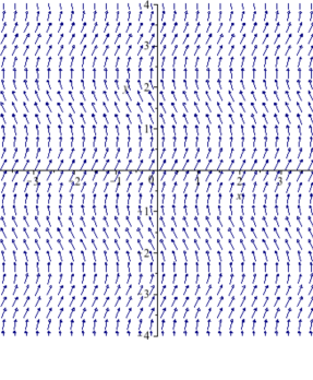
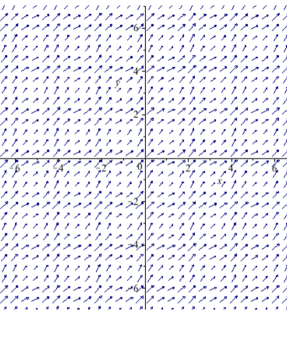
This paper shows that periodic solutions of the compressible gas dynamics equations in two space dimensions exhibit nonuniform dependence on initial conditions, by a mechanism very similar to that governing the incompressible system. Both the constant-density construction of Section 1.1 and the approximate solutions based on the Himonas-Misioล‚ek model take an initial condition consisting of a uniform motion with a smaller oscillatory motion superimposed on it. We sketch the initial velocity fields for typical members of each series in Figure 1. The constant-density and constant-pressure solution is not completely trivial. It is also a solution to the incompressible system, somewhat simpler than the one devised by Himonas and Misioล‚ek. It persists for all time, without the formation of shocks. There may be other families of solutions and approximate solutions with similar structure. The actual solutions corresponding to our approximation (10) do not have constant density or pressure.

Refer to caption
Refer to caption
Figure 1: Velocity Fields for the Constant Density (Left) and Approximate (Right) Solutions

The conclusions to be drawn from this demonstration are of two types. First, โ€œnonuniform dependence on dataโ€ in the sense of this paper can be contrasted to โ€œuniform dependenceโ€ in the sense of Katoโ€™s original well-posedness proof. Second, it is worth calling attention to the nature of the solutions we have constructed, as they are solutions of a hyperbolic system (compressible flow) that is closely related to a system that is not hyperbolic (incompressible flow).

We look at these separately.

4.1 The Meaning of Non-Uniform Dependence

The failure of uniform dependence on the data is instantaneous and is a property of classical solutions. It does not appear to tell us anything about properties of weak solutions (existence of which, for the multidimensional compressible Euler system, is an open problem). In his important paper [9, Theorem III(b)], Kato proves uniform dependence of solutions on the data in the situation where a limiting initial condition in Hssuperscript๐ป๐‘ H^{s} is approximated in Hssuperscript๐ป๐‘ H^{s} by a sequence of initial conditions $\{U_{0}^{n}\}$. That is not the case for our data. While the difference between corresponding terms in our sequences $U^{1,n}$ and $U^{-1,n}$ converges to zero in Hssuperscript๐ป๐‘ H^{s}, neither sequence alone converges in Hssuperscript๐ป๐‘ H^{s}. In verifying the error bounds claimed for the approximate solutions, one can see that the cancellation between the โ€œlow frequencyโ€ terms ($\pm 1/n$ in this case) and the high frequency oscillatory terms is a result of nonlinearities in the system. This creates the possibility of the nonuniformity demonstrated here. A similar type of cancellation, differing in detail, is used in our companion paper [8] to obtain a nonuniformity result for solutions defined on on the plane, rather than on a torus.

4.2 Linear and Nonlinear Behavior in Gas Dynamics

It is also interesting to compare the nonuniform sequences of solutions we have constructed here with the sequences Himonas and Misioล‚ek [7] used in their proof of nonuniform dependence for the incompressible system. That system takes the form of three equations, for velocity and pressure:

$$\nabla\cdot{\bf u}=0\,,\quad{\bf u}_{t}+\nabla\left({\bf u}\times{\bf u}\right)+\nabla p=0\,.$$ (53)

This system is not hyperbolic; to the extent that its characteristics can be compared to those of (1), one could say that the acoustic characteristics in (1) (those associated with the โ€œspeed of soundโ€, and also the pair that are genuinely nonlinear in the sense of conservation laws) have become infinite in (53). (This is more correctly stated in terms of the Mach number โ€“ the ratio of the fluid velocity to the characteristic speed. The system (53) represents a flow in which the Mach number has become zero.)

Our exhibition of nonuniform behavior in a hyperbolic system related to the incompressible system indicates that the nonuniform dependence is

  • (a)

    hyperbolic in nature, and

  • (b)

    based in the linear characteristics of the hyperbolic system, which are shared with the incompressible system โ€“ that is, the shear or entropy waves.

Finally, we observe that a simple adaptation of the constant-density example of Section 1.1 also proves nonuniform dependence on data for the isentropic gas dynamics system โ€“ the system formed from the first three equations of (1) by assuming that the pressure is a given function of the density. That system, of course, has only a single linear family, corresponding to shear waves.

References

  • [1] R.ย A. Adams and J.ย J.ย F. Fournier. Sobolev Spaces, volume 140 of Pure and Applied Mathematics. Elsevier/Academic Press, Amsterdam, 2003.
  • [2] A.ย Bressan. Hyperbolic Systems of Conservation Laws: The One-Dimensional Cauchy Problem. Oxford University Press, Oxford, 2000.
  • [3] C.ย M. Dafermos. Hyperbolic Conservation Laws in Continuum Physics. Springer, Berlin, 2000.
  • [4] L.ย Gรฅrding. Problรจme de Cauchy pour les systรจmes quasi-linรฉaires dโ€™ordre un strictement hyperboliques. In Les ร‰quations aux Dรฉrivรฉes Partielles, volume 117 of Colloques Internationaux du CNRS, pages 33โ€“40. ร‰ditions du Centre National de la Recherche Scientifique, Paris, 1963.
  • [5] A.ย A. Himonas and C.ย Kenig. Non-uniform dependence on initial data for the CH equation on the line. Differential Integral Equations, 22:201โ€“224, 2009.
  • [6] A.ย A. Himonas, C.ย Kenig, and G.ย Misioล‚ek. Non-uniform dependence for the periodic CH equation. Communications in Partial Differential Equations, 35:1145โ€“1162, 2010.
  • [7] A.ย A. Himonas and G.ย Misioล‚ek. Non-uniform dependence on initial data of solutions to the Euler equations of hydrodynamics. Communications in Mathematical Physics, 296:285โ€“301, 2010.
  • [8] J.ย Holmes, B.ย L. Keyfitz, and F.ย TฤฑฤŸlay. Nonuniform dependence on initial data for compressible gas dynamics: The Cauchy problem on ${\mathbb{R}}^{2}$. In preparation.
  • [9] T.ย Kato. The Cauchy problem for quasi-linear symmetric hyperbolic systems. Archive for Rational Mechanics and Analysis, 58:181โ€“205, 1975.
  • [10] H.ย Koch and N.ย Tzvetkov. Nonlinear wave interactions for the Benjamin-Ono equation. International Mathematics Research Notices, 30:1833โ€“1847, 2005.
  • [11] P.ย D. Lax. Hyperbolic Systems of Conservation Laws and the Mathematical Theory of Shock Waves. Society for Industrial and Applied Mathematics, Philadelphia, 1973.
  • [12] J.ย Leray and Y.ย Ohya. Equations et systรฉmes non-linรฉaires, hyperboliques non-stricts. Mathematische Annalen, 170:167โ€“205, 1967.
  • [13] A.ย Majda. Compressible Fluid Flow and Systems of Conservation Laws in Several Space Variables. Springer-Verlag, New York, 1984.
  • [14] A.ย Majda. Smooth solutions for the equations of compressible and incompressible fluid flow. In H.ย Beirรฃo da Veiga, editor, Fluid Dynamics, volume 1074 of Lecture Notes in Mathematics. Springer-Verlag, Berlin, 1984.
  • [15] D.ย Serre. Systems of Conservation Laws. 1: Hyperbolicity, Entropies, Shock Waves. Cambridge University Press, Cambridge, 1999. Translated from the French original by I.ย N.ย Sneddon.
  • [16] M.ย E. Taylor. Partial Differential Equations III: Nonlinear Equations. Springer, New York, 1996.
  • [17] M.ย E. Taylor. Commutator estimates. Proceedings of the American Mathematical Society, 131:1501โ€“1507, 2003.