Geometrical models for the study of astrophysical systems with spheroidal symmetry imbedded in a standard cosmology: The case of cosmic voids.

Abstract

We present a class of general prolate and oblate spheroidal spacetimes for the description of cosmic structures in the Universe. They are exact geometries which represent, in an appropriated way, the imbedding of spheroidal matter-energy distributions within a standard cosmological scenario, and therefore they allow for an improved description of a wider class of astrophysical systems from a more accurate point of view. These spacetimes can be used to describe overdensity or underdensity regions; in this work we consider the last case, that is, the description of cosmic voids. We introduce and study a model of void which is a generalization of a simpler one in spherical symmetry and we use it for the calculation of weak lensing optical scalars as a non-trivial and interesting application. In this particular example we show the rich observable features that can be found in such models.

1 Introduction

In the theoretical modelling of structures of the cosmic matter distribution, the use of spherically symmetric models has been the first natural option employed for the study of such systems. Notably, several astrophysical objects such as galaxy clusters and most cosmic voids are described using this option (See for example [1, 2]). In an standard cosmology, there exists a reason for considering spherically symmetric models; namely, that a priori, in a Robertson-Walker (R-W) background it is natural to expect to find structures with spherical shape since no preferred directions exist in such geometry. However, in our lumpy Universe a great variety of shapes are observed; this fact mainly concerns to the very relevant case of voids.

Cosmic voids are defined as underdensity regions with respect to the mean cosmic energy density $\bar{\varrho}$ of the Universe and they comprise one of the most interesting large scale objects due to its predominant presence in the Universe. Analysis of the 2dF Galaxy Redshift Survey and the Sloan Sky Digital Survey [3, 4] have shown that most part of the Universe is filled out with voids; and about the 40% of its total volume is occupied by voids with radius of the order of 15Mpc [3].

Although very often they do not present very well defined shapes, it have been suggested that a more appropriated characterization of the morphology of voids can be obtained by means of ellipsoids [5, 6, 7]; though in most works the algorithms that search for voids had assumed spherical symmetry.

Dealing with models containing deviations from spherical symmetry confronts the researcher with a considerable increasing of complexity in the description of the system; nevertheless there exists analytic studies[8] using these geometries. However, works found in the literature avoid the use of a detailed metric description for the spacetime of such ellipsoidal configurations inferred from observations. Such kind of models are necessary for several reasons; for example it would allow a more realistic characterization of voids and at the same time they offer the possibility of explore more general energy contents in terms of its whole energy-momentum tensor. This is very interesting taking into account that the nature of the dark sector is actually unknown and that most of the models rest on Newtonian descriptions. Additionally, having exact metrics that describe cosmic voids is relevant for the study of the dynamical aspects of underdensity regions in the problem of evolution and formation of structure in the Universe.

Unfortunately, there is a lack of suitable metrics at our disposal for describing ellipsoidal configurations and therefore the amount of work regarding most sophisticated modeling and its implications is not abundant within the literature.

This work is intended to be a contribution in these directions. Here we present a family of exact metrics in order to model spacetimes of large structures with prolate and oblate spheroidal symmetry imbedded in a standard Robertson-Walker (R-W) cosmology. This means that they are non-perturbative models, and furthermore, they possess two well distinguished regions, namely an inner region which describes a very general class of spheroidal distributions and an outer regions which is chosen to coincide appropriately with an exact isotropic and homogeneous metric. Therefore, they constitute a straightforward generalization of spherically symmetric models surrounded by a cosmological environment. The metrics presented in this article can be used to describe large scale structure as galaxy clusters and cosmic voids; however we will deal in this case with underdensity distributions.

In particular, we analyse below voids with a mass density profile which is an adapted version of a simple model[9] used in spherical symmetry for the study of the probability of detection of weak lensing in the presence of voids. Inspired by reference [9], we use this particular geometric model of a void in a weak lens calculation of the optical scalars in the regime of thin lenses in which we also present an application of the recently reported new expressions for the lens optical scalars in the cosmological context [10].

We have not found in the literature works that use exact spheroidal metrics in a cosmological context to describe voids. Although these geometries constitute a slight modification to spherically symmetric systems, they become quite sophisticated since, for example, the model also allows for non-vanishing spacelike components of the energy-momentum tensor. The reason behind considering this broader assumptions in the degrees of freedom of the matter content comes from the fact that there exist interesting suggestions[11] that such flexibility in the energy content is a valuable alternative to give new insight in the study of the matter content of cosmological and astrophysical systems. This, certainly concerns to voids which are supposed to be one of the typical candidates for the study of the distribution of the cosmic mass-energy content; see for example [12, 13].

Almost all of the information that we have gather for building our cosmological picture, comes from the present past null cone. That is, from each system we are seeing a snapshot. One of the objectives of this work is to communicate a very convenient way to build geometrical models for observed astrophysical system; since it can be shown that the choice of two functions can be used to model a variety of systems with spheroidal symmetry immersed in a cosmological scenario. We will not concentrate in the detailed physical sources of these geometries, but the functions can be chosen so that the usual energy conditions are satisfied[11].

This article is organized as follows. In the next section we recall some elementary geometric relations that will be used in the rest of the article. Section 3 presents the line element of the family of models with different spheroidal symmetry imbedded in a Robertson-Walker cosmology. In section 4 we apply this construction to the modeling of a cosmic void by presenting a metric that have the appropriate geometric behaviour. In section 5 we present the results of the calculation of the optical scalars of this spheroidal void model; which is considered inclined along the line of sight.

2 Geometric Preliminaries

2.1 Spheroids in Euclidean space

There are two natural classes of spheroidal coordinates systems, namely prolate and oblate, and they are generated from elliptic coordinates in the Cartesian plane $\mathbb{R}^{2}$ [14]. Spheroidal coordinates are normally chosen so that its radial coordinate describe a set of confocal spheroids. Prolate spheroidal coordinates are obtained by rotating the confocal ellipses level set along the axis that join the two foci; while that oblate coordinates systems are generated rotating the ellipses level set along an axis perpendicular to the confocal one; this means that after the rotation, the foci draw a ring in the space.

In order to fix the notation, below we introduce both coordinates systems in the usual way trough its relation with Cartesian coordinates $\left(\mathbf{x},\mathbf{y},\mathbf{z}\right)$ in Euclidean space $\mathbb{R}^{3}$.

2.1.1 Prolate spheroidal coordinates

We will denote by $\{r,\theta,\phi\}$ the prolate spheroidal coordinates which have the following domain of definition:

$$r \to[0,\infty),$$ (2.1)

$$\theta \to[0,\pi],$$ (2.2)

$$\phi \to[0,2\pi];$$ (2.3)

and are related to the usual Cartesian coordinates $\left(\mathbf{x},\mathbf{y},\mathbf{z}\right)$ by:

$$\mathbf{x} =r\sin(\theta)\cos(\phi),$$ (2.4)

$$\mathbf{y} =r\sin(\theta)\sin(\phi),$$ (2.5)

$$\mathbf{z} =\sqrt{r^{2}+r^{2}_{\mu}}\cos(\theta);$$ (2.6)

where the constant parameter $r_{\mu}$ has the meaning of the distance of the foci from the origin of the Cartesian coordinate system.

One can see also that surfaces $r=$constant are prolate spheroids with their foci along the $\mathbf{z}-$axis, and therefore satisfy:

$$\frac{\mathbf{z}^{2}}{r^{2}+r^{2}_{\mu}}+\frac{\mathbf{x}^{2}+\mathbf{y}^{2}}{r^{2}}=1;$$ (2.7)

where the value $r=constant$ correspond to the length of its minor radius and the size of its major radius is equal to $\sqrt{r^{2}+r^{2}_{\mu}}$.

In this coordinates system the line element of the flat Euclidean metric in $\mathbb{R}^{3}$ acquires the following expression:

$$ds^{2}=\left(r^{2}+r_{\mu}^{2}\sin(\theta)^{2}\right)\left(\frac{dr^{2}}{r^{2}+r_{\mu}^{2}}+d\theta^{2}\right)+r^{2}\sin(\theta)^{2}\;d\phi^{2}.$$ (2.8)

2.1.2 Oblate spheroidal coordinates

Oblate coordinates are usually labeled by the same set of symbols $\{r,\theta,\phi\}$ employed in the prolate case, and additionally the range of this coordinates is also given by (2.1), (2.2), (2.3).

These coordinates are defined in terms of Cartesian coordinates by

$$\mathbf{x} =\sqrt{r^{2}+r^{2}_{\mu}}\sin(\theta)\cos(\phi),$$ (2.9)

$$\mathbf{y} =\sqrt{r^{2}+r^{2}_{\mu}}\sin(\theta)\sin(\phi),$$ (2.10)

$$\mathbf{z} =r\cos(\theta).$$ (2.11)

The constant parameter $r_{\mu}$ in this case corresponds to the radius described by the foci of the ellipse generating the spheroid when it is rotated around the $\mathbf{z}$-axis.

Let us note that the surfaces $r=$constant describe oblate spheroids with the $\mathbf{z}$ symmetry axis; since one has:

$$\frac{\mathbf{z}^{2}}{r^{2}}+\frac{\mathbf{x}^{2}+\mathbf{y}^{2}}{r^{2}+r^{2}_{\mu}}=1;$$ (2.12)

and where $\sqrt{r^{2}+r^{2}_{\mu}}$ corresponds to the major radius and $r$ the minor one in completely analogy with the prolate case.

The expression of the line element of the flat Euclidean space $\mathbb{R}^{3}$ in terms of oblate coordinates becomes:

$$\begin{split}ds^{2}=\big{(}r^{2}+r_{\mu}^{2}\cos(\theta)^{2}\big{)}\left(\frac{dr^{2}}{r^{2}+r_{\mu}^{2}}+d\theta^{2}\right)+\big{(}r^{2}+r_{\mu}^{2}\big{)}\sin(\theta)^{2}d\phi^{2}.\end{split}$$ (2.13)

2.2 Homogeneous and isotropic spacetime in spheroidal coordinates systems

2.2.1 The standard R-W line element

Since the surrounding geometry of the spheroidal systems are required to be a standard R-W cosmology, before presenting our proposed geometric models we introduce here a description of the R-W metrics in terms of the spheroidal coordinates discussed previously. This form of the line element constitutes the base of the generalized models that we present below.

The line element of a Robertson-Walker Universe can be expressed by

$$ds^{2}=dt^{2}-A(t)^{2}dL_{k}^{2};$$ (2.14)

where $A(t)$ is the expansion parameter and $dL^{2}_{k}$ denotes the line element of an homogeneous and isotropic space with constant curvature; where as usually $k=1,0,-1$ refers to a positive curved, flat and hyperbolic spatial geometries respectively. Among the several equivalent expressions for the line element $dL^{2}_{k}$, we choose the following one which exhibits explicitly the fact that $dL^{2}_{k}$ is conformal to the Euclidean 3-dimensional flat metric

$$dL^{2}_{k}=\frac{1}{\left(1+\frac{k\bar{r}^{2}}{4}\right)^{2}}\left[d\bar{r}^{2}+\bar{r}^{2}\Big{(}d\bar{\theta}^{2}+\sin(\bar{\theta})^{2}d\bar{\phi}^{2}\Big{)}\right].$$ (2.15)

Other usual ways in which $dL^{2}_{k}$ is often expressed are:

$$dL^{2}_{k}= \frac{d\mathtt{r}^{2}}{1-k\mathtt{r}^{2}}+\mathtt{r}^{2}\Big{(}d\bar{\theta}^{2}+\sin(\bar{\theta})^{2}d\bar{\phi}^{2}\Big{)},$$ (2.16)

$$dL^{2}_{k}= d\chi^{2}+f_{k}(\chi)^{2}\Big{(}d\bar{\theta}^{2}+\sin(\bar{\theta})^{2}d\bar{\phi}^{2}\Big{)};$$ (2.17)

where in the last expression $f_{k}(\chi)$ is equal to $\sin(\chi)$ for $k=1$, $\chi$ for $k=0$ or $\sinh(\chi)$ for $k=-1$. However, we prefer to use equation (2.15) since we will exploit its conformal nature using prolate and oblate coordinate system for writing the flat metric inside of the brackets in order to describe spheroidal systems.

2.2.2 The R-W line element in prolate spheroidal coordinates

Using the line element (2.8) together with the relation

$$\bar{r}^{2}\equiv\mathbf{x}^{2}+\mathbf{y}^{2}+\mathbf{z}^{2}=r^{2}+r^{2}_{\mu}\cos(\theta)^{2};$$ (2.18)

which holds for prolate coordinates we obtain for the R-W line element (2.14)

$$\begin{split}ds^{2}=dt^{2}-\frac{A(t)^{2}}{\left[1+\frac{k}{4}\Big{(}r^{2}+r^{2}_{\mu}\cos(\theta)^{2}\Big{)}\right]^{2}}\bigg{[}\left(r^{2}+r_{\mu}^{2}\sin(\theta)^{2}\right)\left(\frac{dr^{2}}{r^{2}+r_{\mu}^{2}}+d\theta^{2}\right)+r^{2}\sin(\theta)^{2}\;d\phi^{2}\bigg{]}.\end{split}$$ (2.19)

2.2.3 The R-W line element in oblate spheroidal coordinates

In this case it is immediate to see that the following relation holds

$$\bar{r}^{2}\equiv\mathbf{x}^{2}+\mathbf{y}^{2}+\mathbf{z}^{2}=r^{2}+r^{2}_{\mu}\sin(\theta)^{2};$$ (2.20)

which together with the line element (2.13) implies

$$\begin{split}ds^{2}=dt^{2}-\frac{A(t)^{2}}{\left[1+\frac{k}{4}\Big{(}r^{2}+r^{2}_{\mu}\sin(\theta)^{2}\Big{)}\right]^{2}}\bigg{[}\left(r^{2}+r_{\mu}^{2}\cos(\theta)^{2}\right)\left(\frac{dr^{2}}{r^{2}+r_{\mu}^{2}}+d\theta^{2}\right)+\big{(}r^{2}+r^{2}_{\mu}\big{)}\sin(\theta)^{2}\;d\phi^{2}\bigg{]}.\end{split}$$ (2.21)

It is probably worthwhile to emphasize that the line elements (2.19) and (2.21) represent the same Robertson-Walker metric (homogeneous and isotropic) in the less conventional spheroidal coordinate systems.

3 Exact spacetime models for spheroidal systems in cosmology

Now, we are in condition to present our models for prolate and oblate spheroidal astrophysical systems imbedded in an standard R-W cosmology.

3.1 Geometry with prolate symmetry

It is possible to generalize the standard homogeneous and isotropic R-W spacetime to one describing a distribution of matter with spheroidal symmetry. This symmetry must be reflected in the geometry of the corresponding spacetime. We do this by introducing two new functions that alter the R-W line element, in a bounded region, but that conforms to the spheroidal symmetry.

For the case of the prolate spheroidal symmetry the proposed line element is:

$$\begin{split}ds^{2}=F(r)dt^{2}-\frac{A(t)^{2}}{\left[1+\frac{k}{4}\Big{(}r^{2}+r^{2}_{\mu}\cos(\theta)^{2}\Big{)}\right]^{2}}\Bigg{[}&\left(r^{2}+r^{2}_{\mu}\sin(\theta)^{2}\right)\Bigg{(}\frac{dr^{2}}{r^{2}-\frac{2M(r)}{r}\Big{(}r^{2}+r^{2}_{\mu}\sin(\theta)^{2}\Big{)}+r^{2}_{\mu}}+d\theta^{2}\Bigg{)}\\ &+r^{2}\sin(\theta)^{2}d\phi^{2}\Bigg{]}.\end{split}$$ (3.1)

3.2 Geometry with oblate symmetry

Applying the same methodology to the case of oblate spheroidal symmetry, we propose the line element:

$$\begin{split}ds^{2}=F(r)dt^{2}-\frac{A(t)^{2}}{\left[1+\frac{k}{4}\Big{(}r^{2}+r^{2}_{\mu}\sin(\theta)^{2}\Big{)}\right]^{2}}\Bigg{[}&\left(r^{2}+r^{2}_{\mu}\cos(\theta)^{2}\right)\Bigg{(}\frac{dr^{2}}{r^{2}-\frac{2M(r)}{r}\Big{(}r^{2}+r^{2}_{\mu}\cos(\theta)^{2}\Big{)}+r^{2}_{\mu}}+d\theta^{2}\Bigg{)}\\ &+\left(r^{2}+r^{2}_{\mu}\right)\sin(\theta)^{2}d\phi^{2}\Bigg{]}.\end{split}$$ (3.2)

One observes the presence of the radial function $M(r)$ in the component $g_{rr}$ of the metric, which we call the mass profile function due to its resemblance with the usual mass function in spherical symmetry, and the presence of the radial function, $F(r)$ which corresponds to the timelike component $g_{tt}$ of the metric. One can see that the spacetime is still foliated by spacelike sections ($t=\text{constant}$) with spheroidal symmetry. It is also clear that if we set $M(r)=0$ and $F(r)=1$ in a region specified by $r>r_{0}$ with $r_{0}=$constant, then, in this outer region, the solution coincides exactly with a R-W geometry, and therefore the dynamics of the scale factor $A(t)$ is determined by the field equations in this region. In the interior region one has a wide range of possible models with spheroidal symmetry which can be adjusted in order to describe several matter-energy distributions.

The mass profile function $M(r)$ is a natural generalization of the mass function in spherical symmetry; in particular it gives the mass content in the limit when $r_{\mu}\to 0$.

The function $F(r)$ is another degree of freedom that one can use to model the physical system. It can be used to introduce non-negligible peculiar spacelike components to the energy-momentum that have shown to be useful for the description of dark matter phenomena [11].

Therefore, the line elements (3.1) and (3.2) constitute a non-trivial class of geometries for the practical study of spheroidal distributions in a cosmological context. We will show their utility in the special case of cosmic under-density regions; in particular we will regard voids from the point of view of weak gravitational lenses and we will perform the computation of the corresponding optical scalars.

4 An exact geometrical model for spheroidal cosmological voids

In this section we present a simple and concrete model for spheroidal voids; that is, a geometry whose associated energy-momentum tensor (via Einstein equations) has a timelike component, namely $T_{t}^{\;\,t}$, which in a given region $r<r_{0}$, is lower than the mean cosmic energy-density in the exterior region $r\geqslant r_{0}$.

If we consider the simple choice $F(r)=1$, then the candidate mass profile function $M(r)$ that one can consider is the one taken from the work [9] which is specified by:

$$M(r)=\begin{cases}\frac{4\pi}{3}\varrho_{\text{int}}r^{3}&\text{for}\quad r<R\\ M(R)+\frac{4\pi}{3}\varrho_{\text{bor}}\left(r^{3}-R^{3}\right)&\text{for}\,R\leq r<R+d\\ 0&\text{for}\quad R+d\leq r;\end{cases}$$ (4.1)

where $\varrho_{\text{int}}$ and $\varrho_{bor}$ are related to the value of mean density outside of the void, namely $\rho_{0}$ and the size parameters $R$ and $d$ in the following way:

$$\varrho_{\text{int}} =-\rho_{0}\epsilon\qquad\qquad\qquad(\text{with}\quad\epsilon\leq 1),$$ (4.2)

$$\varrho_{\text{bor}} =\frac{\rho_{0}\epsilon}{\left(1+\frac{d}{R}\right)^{3}-1}\;\qquad(\text{with}\quad\epsilon\leq 1).$$ (4.3)

The parameter $R$ is associated to the ‘radius’ of the void while the parameter $d$ is related to the size of the wall, that is needed for the compensation. In spherically symmetric cases, this profile is such that the mass at the border compensates for the amount missing in the void and in this way one obtains a compensated void. The value of the density $\rho_{0}$ outside of the voids corresponds to the mean cosmic density which according to the Friedman equation satisfies:

$$\frac{3}{A(t)^{2}}\left[\left(\frac{dA}{dt}\right)^{2}+k\right]=8\pi\rho_{0}.$$ (4.4)

The explicit form of the components of the energy-momentum tensor are quite involved; so that instead of presenting the complicated analytical form of the energy momentum tensor, we show the graph of the energy density in figure 1. It can be seen that our simplified model provides with a a very good description of a region that can be interpreted as an under-density compensated region.

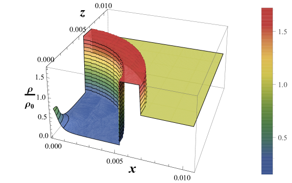
Figure 1: Graphs of the relative energy-density with respect to the mean cosmic density, for a compensated void with prolate spheroidal symmetry, imbedded in a Robertson-Walker spacetime; with symmetry axis along the $z$ direction. We have used the geometric parameters $d=0.3R$, $\epsilon=0.9$, $r_{\mu}=0.1R$, with a radius $R$ corresponding to a physical size of 22Mpc.

5 Weak gravitational lensing of spheroidal voids

5.1 General thin lens equations

In this section we present the numeric computation of the optical scalars when we regard the void as a weak thin lens.

Our calculations make use of the weak lensing formalism developed in [15, 10] where new expressions for the optical scalars describing the distortion of images by the weak gravitational field of a general distribution were reported. These expressions have the advantage of including the whole energy-momentum tensor in the description of the lens in contrast to the formalism usually employed which is based in the linear superposition of massive point like deflectors.

In the cosmological context the convergence $\kappa$ and shear components $\left(\gamma_{1},\gamma_{2}\right)$ of a thin lens are given by[10]

$$\kappa =\left(1-\kappa_{c}\right)\kappa_{L}+\kappa_{c},$$ (5.1)

$$\gamma_{1}+i\gamma_{2} =\left(1-\kappa_{c}\right)(\gamma_{1L}+i\gamma_{2L});$$ (5.2)

with

$$\kappa_{L} =\textbf{D}_{ls}\int_{\lambda_{l}}^{\lambda_{s}}\delta\Phi_{00}\,d\lambda,$$ (5.3)

$$\gamma_{1L}+i\gamma_{2L} =\textbf{D}_{ls}\int_{\lambda_{l}}^{\lambda_{s}}\delta\Psi_{0}\,d\lambda;$$ (5.4)

where $\delta\Phi_{00}$ and $\delta\Psi_{0}$ represent the departure of the components $\Phi_{00}$ and $\Psi_{0}$ of the Ricci tensor and the Weyl tensor from the R-W geometry; $\lambda$ denotes the affine parameter along the null geodesics and the cosmological convergence $\kappa_{c}$ together with the factor $\textbf{D}_{ls}$ are given by:

$$\kappa_{c}=1-\frac{D_{A}(\lambda)}{\lambda},$$ (5.5)

$$\textbf{D}_{ls}=\frac{1}{1+z_{l}}\frac{D_{A_{sl}}D_{A_{l}}}{D_{A_{s}}};$$ (5.6)

where $D_{A}$ denotes angular diameter distances and $z$ the cosmological redshift; the subindex $s$ and $l$ refer to the source and the lens respectively (For details we refer the reader to [10]).

5.2 Optical scalars for a prolate spheroidal void tilted with respect to the line of sight

In our calculation we take into account the possibility that the spheroidal geometry is tilted with respect to the line of sight by an angle $\iota$. We adopt the convention that the plane of the lens which is locate at the cosmological distance $\lambda_{l}$, correspond to the plane $y=0$ in the local reference system associated to the spheroid in which it is inclined with respect to the vertical $z$-axis as it is show in the figure 2.

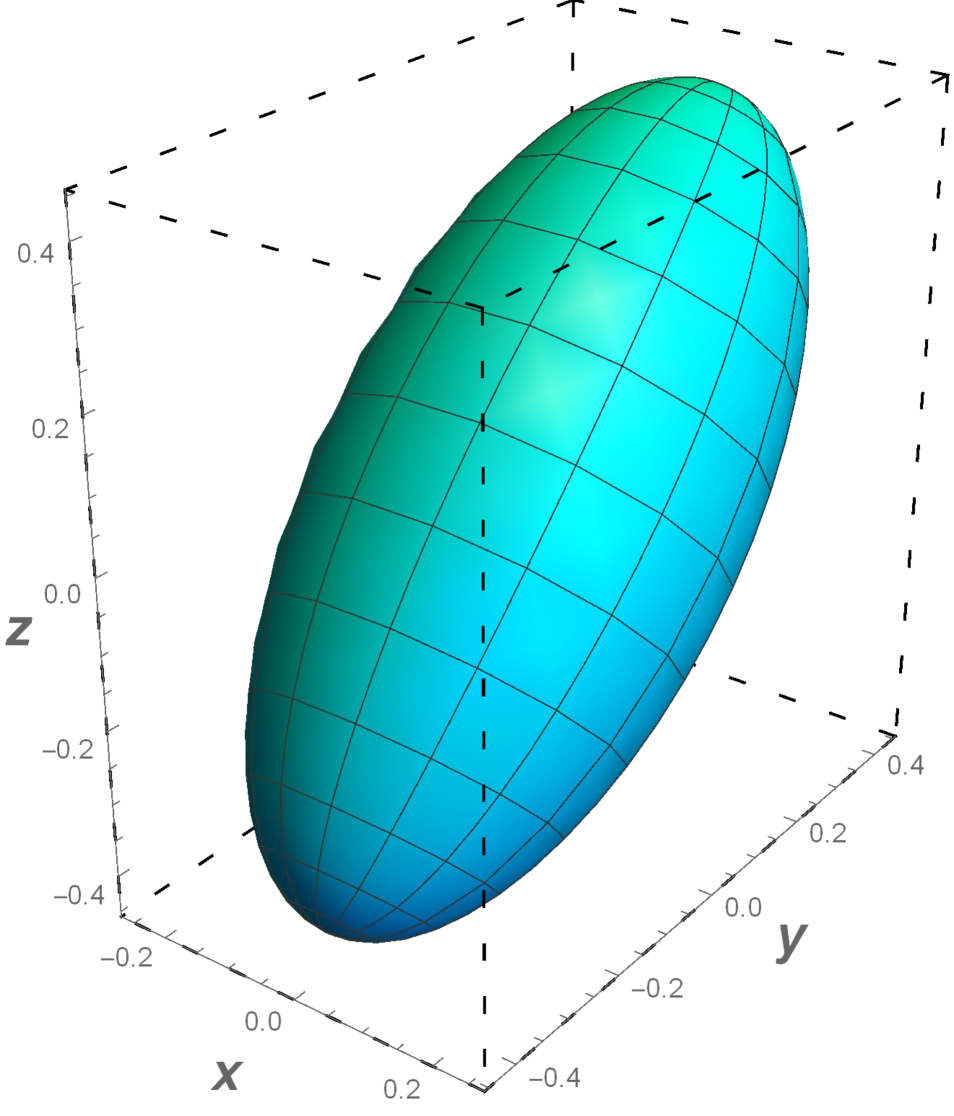
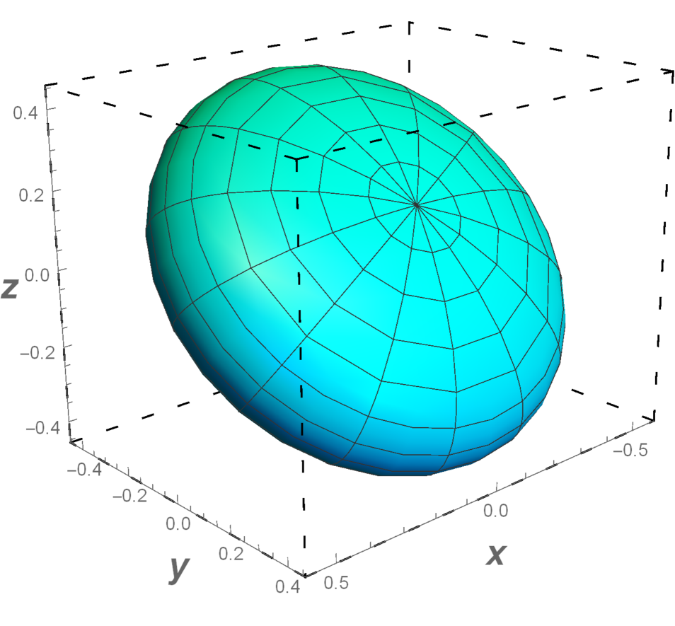
Figure 2: Tilted prolate and oblate spheroids. Photons travel approximately along the $y$ direction which is the line of sight of the observer.

Working in the thin lens approximation is consistent with the assumption that the time of flight of the photons, in the void, is negligible in comparison with the cosmological distance traveled in the R-W geometry; therefore, for all practical purposes one can consider the geometry of the spheroidal lens as static; in other words, we assume that while the photons travel along the void, the expansion parameter has the constant value $A_{\mathbf{v}}$.

In this section we will consider a timelike component of the metric $F(r)\neq 1$. The function $F(r)$ that we have chosen is an adapted version of the one appearing in the timelike component of a spherically symmetric peculiar geometry presented in the work [11]. Such functional form plays a key role in the description of many of the characteristic phenomenology observed in astrophysical system with dark matter[11]; and it is given by

$$F(r)=F_{0}\left[C+\ln\left(\frac{r}{r_{\mu}}+\sqrt{1+\frac{r^{2}}{r_{\mu}^{2}}}\right)\right]^{2};$$ (5.7)

where $F_{0}$ and $C$ are both constant parameters. The main feature that introduces this particular functional dependence is that the spacelike components of the energy-momentum tensor become non-negligible with respect to the timelike one and therefore it produces a significant contribution which is reflected in weak lensing calculations.

The following results correspond to a prolate spheroidal void which is tilted an angle $\iota=\frac{\pi}{4}$ with respect to the line of sight. It has a typical size such as those found in catalogs (as for example in [3]). Below we give the detailed values used in this numerical calculation. The parameter $R$ in equation (4.1) was chosen so that the void has a typical radius of about 20Mpc, the parameter $d$ controlling the width of the walls has been taken as $d=0.3R$, while $r_{\mu}$ corresponds to 3Mpc. The parameter $\epsilon$, also involved in equation (4.1) was taken equal to 0.9.

The selection of the constants $C$ in (5.7) was made ensuring that the component $T_{r}^{\;r}$ of the energy-momentum tensor remains of the same order as the mean density cosmic density $\rho_{0}$; in our case $C=10^{7}$.

The cosmology employed was a $\Lambda$CDM with cosmological parameters taken from the values reported by the Planck Collaboration [16] and the factor $\textbf{D}_{ls}$ was taken $\sim 220\text{Mpc}$.

Below we show the graphs of the optical scalar $\kappa_{L}$, the components $\gamma_{1L}$ and $\gamma_{2L}$ of the shear, and of its module $\gamma$ for a prolate spheroidal distribution. The relation among the components of the shear and its module is expressed by

$$\gamma_{1}+i\gamma_{2}\equiv-\gamma e^{i2\vartheta};$$ (5.8)

where the phase $\vartheta$ has the meaning of an angle in the plane $x-z$ of the lens.

In the case of spheroids the phase $\vartheta$ has a complicated relation in terms of the impact position in the lens plane which can be seen by inspection of the individual components $\left(\gamma_{1},\gamma_{2}\right)$.

Figure 3: Graphs of the optical scalars in terms of coordinates of the plane of the lens for a prolate spheroidal void tilted $\iota=\frac{\pi}{4}$ respect to the line of sight. Left: the optical scalar parameter $\kappa$. Right: the module of the shear $\gamma$.

Figure 4: It can be seen that both components of the shear show a rich structure, that obviously disappear outside the void. Left: Real component of the shear $\gamma_{1L}$. Right: Imaginary component of shear $\gamma_{2L}$.

One can see that the magnitude of the optical scalar functions for the case of typical voids imbedded in a cosmological scenario is very small in agreement with previous analysis [9].

It can be observed that the behaviour of the shear shows a rich structure, and that neither the component nor the norm follow an expected quasi elliptical shape, coming from a projected spheroidal symmetric distribution. Instead, when one looks at the behavior of the convergence $\kappa$, shown in figure (3), it can be seen a simpler behaviour.

6 Final comments

In this work on exact geometries with spheroidal symmetry which are suitable imbedded in a standard cosmological model, we have presented a very broad class of metrics useful for the description of over and underdensities matter distributions, namely equations (3.1) and (3.2). These geometries are characterized by two ‘radial’ functions which can be set appropriately to give a R-W geometry in the range $r\geqslant r_{0}$, for some prescribed fixed comoving radius $r_{0}$; while the internal region $r<r_{0}$ is interpreted to represent an spheroidal system which grow with the expansion factor $A(t)$. The two scalars have a direct physical interpretation; the function $M(r)$ which was chosen such that in th limit $r_{\mu}\to 0$ coincides with the usual mass in spherical symmetry, has also here a close relation with the energy density of the spheroidal distributions, as can be seen from inspection of figure 1. The function $F(r)$ has been used in the past to model peculiar spacelike components of the energy-momentum tensor; which are useful for the description of dark matter phenomena[11].

Using these exact geometries, we have presented a model of void which admits within its interior region ($r<r_{0}$) an energy-momentum tensor which posses non-trivial components in general. We have not found in the literature other presentations of exact metrics that represent a cosmic void imbedded in an homogeneous cosmological Universe with spheroidal symmetry. This model is at the same time an extension of a simple radial profile[9] employed for spherical voids. It has been shown that effectively it can be used as an appropriated model for representing underdensity distributions in a non-perturbative way.

As an interesting application we have taken the case of prolate spheroids for performing a weak lensing analysis in the usual thin lens approximation. Our calculation makes use of the techniques presented in [10] for computing the optical scalars of the lens. In this example we have seen that although the expected signal is rather low, some non-trivial features are displayed; for instance, the shear field does not recreate the expected quasi-elliptical geometry of a projected ellipsoid in the lens plane such as shown in section 5.

We expect that the geometries presented here will be very useful in the study of systems requiring a more sophisticated modeling than the usual spherical assumption; specially in the case of voids where the need for more general descriptions of their geometry seems very demanding.

In the future we plan to apply these type of models to the description of specific observations of astrophysical systems.

References

- [1] N. Hamaus, P. Sutter and B. D. Wandelt, A Universal Density Profile for Cosmic Voids, 1403.5499.
- [2] K. T. Inoue and J. Silk, Local Voids as the Origin of Large-angle Cosmic Microwave Background Anomalies: The Effect of a Cosmological Constant, Astrophys. J. 664 (2007) 650–659, [astro-ph/0612347].
- [3] F. Hoyle and M. S. Vogeley, Voids in the 2dF Galaxy Redshift Survey, Astrophys.J. 607 (2004) 751–764, [astro-ph/0312533].
- [4] D. C. Pan, M. S. Vogeley, F. Hoyle, Y.-Y. Choi and C. Park, Cosmic Voids in Sloan Digital Sky Survey Data Release 7, Mon.Not.Roy.Astron.Soc. 421 (2012) 926–934, [1103.4156].
- [5] C. Foster and L. A. Nelson, The Size, Shape and Orientation of Cosmological Voids in the Sloan Digital Sky Survey, Astrophys. J. 699 (2009) 1252–1260, [0904.4721].
- [6] A. V. Tikhonov and I. D. Karachentsev, Minivoids in the Local Volume, Astrophys.J. 653 (2006) 969–976, [astro-ph/0609109].
- [7] R. van de Weygaert and E. Platen, Cosmic Voids: structure, dynamics and galaxies, Int. J. Mod. Phys. Conf. Ser. 01 (2011) 41–66, [0912.2997].
- [8] D. Park and J. Lee, The Void Ellipticity Distribution as a Probe of Cosmology, Phys. Rev. Lett. 98 (2007) 081301, [astro-ph/0610520].
- [9] L. Amendola, J. A. Frieman and I. Waga, Weak Gravitational lensing by voids, Mon. Not. Roy. Astron. Soc. 309 (1999) 465, [astro-ph/9811458].
- [10] E. F. Boero and O. M. Moreschi, Gravitational lens optical scalars in terms of energy-momentum distributions in the cosmological framework, 1610.06032.
- [11] E. Gallo and O. Moreschi, Peculiar anisotropic stationary spherically symmetric solution of Einstein equations, Mod.Phys.Lett. A27 (2012) 1250044, [1111.0327].
- [12] S. Gottloeber, E. L. Lokas, A. Klypin and Y. Hoffman, The Structure of voids, Mon. Not. Roy. Astron. Soc. 344 (2003) 715, [astro-ph/0305393].
- [13] P. Melchior, P. M. Sutter, E. S. Sheldon, E. Krause and B. D. Wandelt, First measurement of gravitational lensing by cosmic voids in SDSS, Mon. Not. Roy. Astron. Soc. 440 (2014) 2922–2927, [1309.2045].
- [14] P. Moon and D. Spencer, Field theory handbook: including coordinate systems, differential equations, and their solutions. Springer-Verlag, 1988.
- [15] E. Gallo and O. M. Moreschi, Gravitational lens optical scalars in terms of energy- momentum distributions, Phys. Rev. D83 (2011) 083007, [1102.3886].
- [16] Planck collaboration, P. A. R. Ade et al., Planck 2015 results. XIII. Cosmological parameters, Astron. Astrophys. 594 (2016) A13, [1502.01589].