A CHEMICAL COMPOSITION SURVEY OF THE IRON–COMPLEX GLOBULAR CLUSTER NGC 6273 (M 19)

Abstract

Recent observations have shown that a growing number of the most massive Galactic globular clusters contain multiple populations of stars with different [Fe/H] and neutron–capture element abundances. NGC 6273 has only recently been recognized as a member of this “iron–complex” cluster class, and we provide here a chemical and kinematic analysis of $>$ 300 red giant branch (RGB) and asymptotic giant branch (AGB) member stars using high resolution spectra obtained with the Magellan–M2FS and VLT–FLAMES instruments. Multiple lines of evidence indicate that NGC 6273 possesses an intrinsic metallicity spread that ranges from about [Fe/H] = –2 to –1 dex, and may include at least three populations with different [Fe/H] values. The three populations identified here contain separate first (Na/Al–poor) and second (Na/Al–rich) generation stars, but a Mg–Al anti–correlation may only be present in stars with [Fe/H] $\gtrsim$ –1.65. The strong correlation between [La/Eu] and [Fe/H] suggests that the s–process must have dominated the heavy element enrichment at higher metallicities. A small group of stars with low [$\alpha$/Fe] is identified and may have been accreted from a former surrounding field star population. The cluster’s large abundance variations are coupled with a complex, extended, and multimodal blue horizontal branch (HB). The HB morphology and chemical abundances suggest that NGC 6273 may have an origin that is similar to $\omega$ Cen and M 54.

1. INTRODUCTION

Galactic globular clusters are no longer considered pure simple stellar populations. Although large and often (anti–)correlated star–to–star light element abundance variations have long been known to exist within individual globular clusters (e.g., Cohen 1978; Peterson 1980; Cottrell & Da Costa 1981; Sneden et al. 1991; Pilachowski et al. 1996a; Kraft et al. 1997; Shetrone & Keane 2000; Gratton et al. 2001; Ivans et al. 2001), the ubiquitous nature of their peculiar chemical compositions has only recently been recognized. Large sample spectroscopic surveys have revealed that all but perhaps the lowest mass clusters (Walker et al. 2011; Villanova et al. 2013; Salinas & Strader 2015) exhibit similar, but not identical, (anti–)correlations among elements ranging from carbon to aluminum (e.g., Carretta et al. 2009a, 2009b; Mészáros et al. 2015). In many cases, He enhancements coincide with increased abundances of N, Na, and Al and decreased abundances of C, O, and Mg (e.g., Bragaglia et al. 2010a, 2010b; Dupree et al. 2011; Pasquini et al. 2011; Villanova et al. 2012; Marino et al. 2014a; Mucciarelli et al. 2014). Except for CN variations due to in situ mixing, these interconnected light element abundance patterns may be unique to old ($\gtrsim$ 6 Gyr) globular cluster environments (e.g., Pilachowski et al. 1996b; Sneden et al. 2004; Mucciarelli et al. 2008; Bragaglia et al. 2014).

Large light element abundance variations can have a significant effect on a star’s structure and spectrum (e.g., see Piotto et al. 2015; their Figure 1), and recent near UV observations from the Hubble Space Telescope (HST) have exploited this property to reveal a further connection between chemical compositions and globular cluster formation. A key observational constraint for globular cluster formation scenarios is whether the range of light element abundances follows a continuous distribution or falls into discrete groups. Although some purely spectroscopic evidence supports clusters hosting discrete groups with unique light element chemistry (e.g., Carretta et al. 2009a, 2014; Johnson & Pilachowski 2010; Carretta 2014, 2015; Cordero et al. 2014; Roederer & Thompson 2015), HST photometry has been particularly efficient at showing that most or all Galactic globular clusters host multiple distinct populations rather than continuous distributions (e.g., Piotto et al. 2007, 2015; Bragaglia et al. 2010a; Milone et al. 2013, 2015a, 2015b; Marino et al. 2016). The combined data from spectroscopy and photometry provide strong evidence that globular clusters experienced multiple rounds of star formation. However, the detailed processes by which globular clusters form, and the nucleosynthetic origins of the light element abundance variations, remain unresolved issues (e.g., see recent discussions in Valcarce & Catelan 2011; Bastian et al. 2015; Bastian & Lardo 2015; Renzini et al. 2015; D’Antona et al. 2016)

Despite most globular clusters exhibiting large light element abundance variations, most systems do not display the same complexity for the heavier elements. The [Fe/H] and [X/Fe] ratios for most $\alpha$ and Fe–peak elements vary by $\sim$0.1 dex or less within an individual cluster (e.g., Carretta et al. 2009c), but intrinsic variations at the few percent level may be present for all elements (Yong et al. 2013). Some clusters exhibit primordial abundance variations for elements produced by the rapid neutron–capture process (r–process), but many do not (e.g., Roederer 2011). Most clusters also fail to show chemical signatures of extended star formation histories, such as elevated slow neutron–capture (s–process) abundances or low [$\alpha$/Fe] ratios. More metal–rich clusters tend to exhibit stronger s–process signatures (e.g., higher average [Ba/Eu] or [La/Eu] ratios) than their more metal–poor counterparts (e.g., Simmerer et al. 2003; Gratton et al. 2004; James et al. 2004; Cohen & Meléndez 2005; Carretta et al. 2007; D’Orazi et al. 2010; Worley & Cottrell 2010), but these differences are likely driven by the broader chemical enrichment of the Galaxy.

Interestingly, a growing number of clusters have been discovered that exhibit chemical and morphological characteristics consistent with extended star formation histories, and may represent a new class of objects. These “iron–complex” clusters are characterized as having: (1) broadened or multimodal [Fe/H] distribution functions with dispersions exceeding $\sim$0.1 dex when measured using high resolution spectra; (2) complex color–magnitude diagrams and split RGB sequences when observed with hk narrow band photometry (e.g., Lee 2015; Lim et al. 2015); (3) and correlated abundances of [Fe/H] and elements likely produced by the main s–process (e.g., Ba and La). To date, $\sim$10 iron–complex clusters have been discovered (e.g., see Da Costa 2016a, their Table 1; Marino et al. 2015, their Table 10). Many of these systems also have about the same metallicity ([Fe/H] $\sim$ –1.7), have very blue and extended horizontal branch (HB) morphologies, and are among the most massive clusters in the Galaxy (M_V $\lesssim$ –8). The iron–complex cluster M 54 may be the nuclear star cluster of the Sagittarius dwarf galaxy (e.g., Bellazzini et al. 2008), and the most massive iron–complex cluster omega Centauri ($\omega$ Cen) is strongly suspected to be a stripped dwarf galaxy nucleus as well (e.g., Bekki & Freeman 2003). Similarly, the iron–complex clusters NGC 1851 and M 2 may also be the stripped cores of former dwarf galaxies (e.g., Olszewski et al. 2009; Kuzma et al. 2016). Therefore, iron–complex clusters may be the relics of more massive systems, the remnants of previous Milky Way accretion events, and/or trace a particular time or accretion period in the Galaxy’s formation history.

Among the iron–complex cluster class, $\omega$ Cen, M 54 and the Sagittarius system, M 2, NGC 5286, and NGC 6273 (M 19) stand out as particularly interesting. These clusters exhibit broad metallicity distributions with discrete populations occurring near the same [Fe/H] values, and also host trace populations of metal–rich stars with peculiar chemical compositions (e.g., Pancino et al. 2002; Carretta et al. 2010a; Johnson & Pilachowski 2010; Marino et al. 2011a, 2015; McWilliam et al. 2013; Yong et al. 2014; Johnson et al. 2015a). In order to investigate this phenomenon further, we have obtained high resolution spectra of $>$ 800 red giant branch (RGB) and asymptotic giant branch (AGB) stars located near the massive bulge cluster NGC 6273. Following Johnson et al. (2015a), Han et al. (2015), and Yong et al. (2016), we aim to investigate the cluster’s metallicity distribution function and trace the cluster’s detailed chemical composition across its various stellar populations.

2. OBSERVATIONS AND DATA REDUCTION

2.1. Magellan Spectroscopic Data

In Johnson et al. (2015a), we identified an intrinsic metallicity spread in NGC 6273, and noted the existence of several stars redder than the formal RGB that could belong to an even more metal–rich component. Since the previous observations were restricted to the color range 0.7 $\leq$ J–K_S $\leq$ 1.0 on the upper RGB, we expanded the target selection criteria for the new observations to include stars in the color range 0.6 $\leq$ J–K_S $\leq$ 1.3. The new observations also span luminosities from the HB to the RGB–tip, and range from 0.53–13.98$\arcmin$ in projected distance from the cluster center (see Figure 1). However, stars closer to the cluster center were given higher priorities in the target ranking process. All coordinates and photometry for the target selection process were taken from the Two Micron All Sky Survey (2MASS; Skrutskie et al. 2006) database.

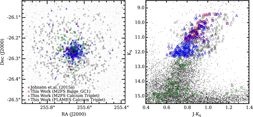
Figure 1.— Left: the sky coordinates of all targets observed for this work and Johnson et al. (2015a) are superimposed on a 2MASS (Skrutskie et al. 2006) J–band image centered on NGC 6273. The black, red, blue, and green symbols indicate stars that are radial velocity members, and the grey symbols indicate stars that are likely not cluster members. Right: a 2MASS J–K_S color–magnitude diagram is shown with the NGC 6273 member and non–member stars indicated using the same symbol and color designations as in the left panel.

In order to efficiently obtain a large number of high resolution spectra, we employed the Michigan/Magellan Fiber System (M2FS; Mateo et al. 2012) and MSpec multi–object spectrograph mounted on the Magellan–Clay 6.5m telescope. In single order mode, M2FS is capable of placing 256 1.2$\arcsec$ fibers on targets across a nearly 30$\arcmin$ field–of–view. However, additional orders can be observed simultaneously using a cross–disperser, at the expense of fewer targets. We utilized both options for this project. The first setup operated in single order mode and was optimized to observe the 8542 Å and 8662 Å near–infrared Calcium II Triplet (CaT) lines. These data provided radial velocities and CaT metallicities for 466 stars, and permitted an investigation into the full spatial, color, and metallicity extent of NGC 6273. The second setup (“Bulge$\_$GC1” filter) included 6 consecutive orders, spanned 6120–6720 Å, allowed for up to 48 fibers to be allocated per configuration, and was used to obtain radial velocities and detailed chemical abundances for 82 stars. As can be seen in Figure 1, both data sets spanned broad color and radial distance ranges, but the CaT data extended to fainter stars.

Both instrument setups utilized a four amplifier slow readout mode and were binned 2 $\times$ 1 (spatial $\times$ dispersion). The CaT and Bulge$\_$GC1 observations were taken with the 180$\mu$m (widest) and 125$\mu$m slits, respectively. However, both setups yielded approximately the same resolving power of R $\equiv$ $\lambda$/$\Delta$$\lambda$ $\approx$ 27,000, based on an examination of the ThAr wavelength calibration spectra. The two CaT fields were observed for a total of 10,200 seconds, and the two Bulge$\_$GC1 fields were observed for a total of 21,600 seconds. A summary of the observation dates, instrument configurations, and integration times is provided in Table 1.

For data reduction, we followed the procedures outlined in Johnson et al. (2015b; see their Section 2.3). Briefly, we used standard IRAF tasks to apply the bias correction, trim the overscan regions, correct for dark current, and combine the individual amplifier images from each CCD into single images. The IRAF dohydra task was used for aperture identification and tracing, flat–field correction, scattered light removal, wavelength calibration, cosmic ray removal, and spectrum extraction. For the CaT data, we did not apply any corrections for fringing beyond the flat–field correction. A master sky spectrum was created for each exposure by combining the individual sky fiber spectra. The target spectra were then sky corrected using the skysub routine. Finally, the individual extracted spectra for each star were co–added separately, normalized with the continuum routine, and corrected for telluric absorption lines using the telluric task. Typical signal–to–noise (S/N) ratios ranged from about 20–100 per pixel for the CaT data and 30–100 per pixel for the Bulge$\_$GC1 data.

2.2. Very Large Telescope Spectroscopic Data

We supplemented the M2FS CaT data set with additional observations of 300 RGB stars taken with the Very Large Telescope (VLT) FLAMES–GIRAFFE instrument. The data were downloaded from the European Southern Observatory (ESO) Science Archive Facility under request number 210062. The FLAMES observations spanned a broad range of magnitudes, but were generally fainter than the M2FS data. However, the spatial coverage between the two data sets was similar (see Figure 1). Note that we have only included stars for which we could identify a 2MASS source within 2$\arcsec$ of the coordinates provided in the image headers.

All of the FLAMES–GIRAFFE observations were obtained using the HR21 setup, which provides R $\approx$ 18,000 spectra from 8482–9000 Å. However, we only analyzed the region spanning 8500–8700 Å, which is similar to the M2FS–CaT data and includes the same 8542 Å and 8662 Å CaT features. The observations were taken via six configurations, each with an integration time of 2445 seconds. Most stars were observed in two configurations, but not always with the same fiber each time. A small number of stars were observed in three or more configurations, and a few were observed only once. A summary of the observation dates for each configuration is provided in Table 1.

The data were primarily reduced using the GIRAFFE Base–Line Data Reduction Software (girBLDRS) package. The girBLDRS suite was used to carry out basic CCD processing tasks (e.g., bias correction and overscan trimming) and also the more advanced multi–fiber tasks we performed with dohydra for the M2FS data (see Section 2.1). Similar to the M2FS CaT data, we did not apply any further corrections for fringing beyond the flat–field correction. The sky subtraction, continuum normalization, and spectrum combining were carried out with the same IRAF routines as used for the M2FS data. However, since the FLAMES data were obtained over the course of several weeks to months, we applied the heliocentric velocity corrections provided in the image headers before combining the multiple exposures. The final S/N values are comparable to those of the M2FS CaT data.

2.3. HST Imaging Data

NGC 6273 is known to have a broad RGB and a peculiar HB morphology that is similar to $\omega$ Cen (Piotto et al. 1999; Momany et al. 2004; Brown et al. 2010, 2016; Han et al. 2015). Therefore, in support of our spectroscopic observations we have obtained new HST Wide Field Camera 3 UVIS channel (WFC3/UVIS) data centered on NGC 6273 that includes the F336W, F438W, F555W, and F814W filters. The observations were split into a series of short and long exposures, taken over the course of 4 orbits, that ranged in duration from 10–685 seconds. A post–flash of 2.0–4.7 seconds was included for all exposures, and the BLADE = A option was set for all of the 10 second exposures to minimize shutter–induced vibration (see Section 6.11.4 of the WFC3 handbook). A summary of the filter choices, integration times, and observation dates is provided in Table 1.

The basic data reductions were carried out by the Space Telescope Science Institute’s WFC3 pipeline, but we only performed analyses on the CTE–corrected flc images. All photometry was obtained using the DOLPHOT (Dolphin 2000) package and its associated WFC3 module. The DOLPHOT parameters closely followed the values recommended by Williams et al. (2014) and provided by the DOLPHOT/WFC3 documentation for point sources in crowded fields. No special attempt was made to recover saturated stars; however, only a small number of the brightest stars, predominantly in the F814W filter, were lost due to saturation.

As noted by several previous authors (Racine 1973; Harris et al. 1976; Piotto et al. 1999; Davidge 2000; Valenti et al. 2007; Brown et al. 2010; Alonso–García et al. 2012), differential reddening is a significant concern along lines–of–sight near NGC 6273. Previous work estimated that the cluster has E(B–V) = 0.31–0.47 magnitudes and $\Delta$E(B–V) $\sim$ 0.2–0.3 magnitudes. We observe a similar reddening range of $\Delta$E(B–V) = 0.36 magnitudes using corrections kindly provided by A. Milone (2016, private communication; see also Milone et al. 2012 for an outline of the dereddening procedure) via the F336W and F814W data sets. Additionally, we find that adopting an absolute color excess of E(B–V) = 0.37 magnitudes places the coolest HB stars at approximately the correct F555W magnitude, assuming a distance of 9 kpc (Piotto et al. 1999). Further details regarding the photometric analysis, including the dereddening procedure, will be provided in a future publication. However, in Figure 2 we show the smoothed reddening map of the WFC3 field, and include several dereddened color–magnitude diagrams with the radial velocity members identified.

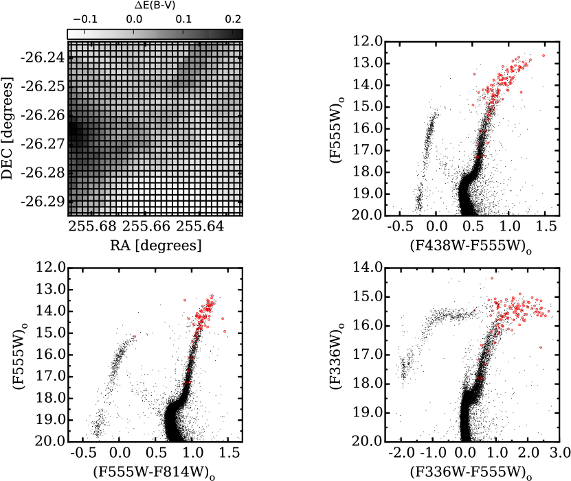
Figure 2.— The top left panel illustrates the spatial variations in differential reddening, $\Delta$E(B–V), across the WFC3 field of NGC 6273, and is in good agreement with the map provided by Alonso–García et al. (2012). Note that the high reddening region on the eastern side of the cluster core correlates with the known position of an interstellar cloud (e.g., Harris et al. 1976). The remaining panels show dereddened color–magnitude diagrams using combinations of the F336W, F438W, F555W, and F814W filters. The open red circles indicate stars from our sample and Johnson et al. (2015) that have radial velocities consistent with cluster membership. All WFC3 photometry is on the VEGAMAG system.

3. RADIAL VELOCITIES AND CLUSTER MEMBERSHIP

Radial velocities were measured for all M2FS and FLAMES spectra using the XCSAO (Kurtz & Mink 1998) cross–correlation code. The velocities were measured relative to a synthetic stellar spectrum of an evolved RGB star with [Fe/H] = –1.60, which is approximately the average metallicity of NGC 6273 (Johnson et al. 2015a). The template spectrum was smoothed and rebinned to match the resolution and sampling of the observed spectra. Heliocentric velocity corrections were calculated with IRAF’s rvcorrect utility for the M2FS data, and for the FLAMES data we used the corrections provided in the image headers. The heliocentric corrections were applied to all of the spectra before being measured with XCSAO.

For the Bulge$\_$GC1 spectra, we measured the velocities using the 6140–6270 Å window because it contains several lines suitable for cross–correlation but avoids very broad lines (e.g., H$\alpha$) and any residual telluric features. For the M2FS and FLAMES CaT data, we used the full spectral window from 8500–8700 Å, but avoided the strong CaT lines. A histogram of the heliocentric radial velocity (RV_helio.) distributions for each data set, including data from Johnson et al. (2015a), is shown in Figure 3. Using these data, we considered stars with RV_helio. between $+$120 and $+$170 km s^-1 to be cluster members. Therefore, the new Bulge$\_$GC1, M2FS CaT, and FLAMES CaT data provided average velocities and dispersions of $+$143.15 km s^-1 ($\sigma$ = 9.53 km s^-1), $+$144.74 km s^-1 ($\sigma$ = 8.79 km s^-1), and $+$145.76 km s^-1 ($\sigma$ = 7.12 km s^-1), respectively, for the cluster members. Similarly, the average RV_helio. value for the combined data sets is $+$144.71 km s^-1 ($\sigma$ = 8.57 km s^-1), which is in good agreement with recent measurements (Johnson et al. 2015a; Yong et al. 2016). For the non–member stars, we found the average velocity and dispersion to be –29.36 km s^-1 and $\sigma$ = 77.02 km s^-1. These values are in agreement with previous kinematic observations of similar off–axis bulge fields (e.g., Kunder et al. 2012; Ness et al. 2013a; Zoccali et al. 2014).

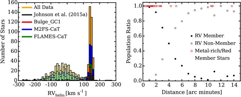
Figure 3.— Left: a radial velocity histogram is shown for all of the spectroscopic data sets used here. Stars with heliocentric radial velocities between $+$120 and $+$170 km s^-1 were considered cluster members, and are indicated by the dark colored histograms. The light colored histograms show the radial velocity distributions of the non–members. The data are sampled in 10 km s^-1 bins. Right: a plot of the member/non–member ratio as a function of the projected distance from the cluster center. Cluster membership was assigned using a star’s heliocentric radial velocity. The open red boxes indicate the projected radial distances for radial velocity member stars with [Fe/H] $>$ –1.35 and/or that lie redward of the dominant RGBs seen in Figures 1 and 2.

The average RV_helio. uncertainties are 0.31 km s^-1 ($\sigma$ = 0.27 km s^-1), 1.09 km s^-1 ($\sigma$ = 0.69 km s^-1), and 0.88 km s^-1 ($\sigma$ = 0.06 km s^-1) for the Bulge$\_$GC1, M2FS CaT, and FLAMES CaT data, respectively. These values represent the measurement uncertainties from the XCSAO cross–correlation routine. However, 57 stars were observed in at least two different setups, including the data from Johnson et al. (2015a), and we measured an average dispersion between repeat measurements of 1.31 km s^-1. If we ignore the four outliers with dispersions $>$ 5 km s^-1, the average dispersion decreases to 0.88 km s^-1. Therefore, we regard $\sim$1 km s^-1 as a reasonable estimate of the systematic uncertainty due to the use of different instruments, configurations, and wavelength regions.

As can be seen in Figure 3, the systemic cluster velocity is well separated from the broad field star distribution of the Galactic bulge. From the Bulge$\_$GC1, M2FS CaT, and FLAMES CaT data, we found 59/82 (72$\%$), 191/466 (41$\%$), and 83/300 (28$\%$) stars to have velocities consistent with cluster membership, respectively. The significantly higher membership rate for the Bulge$\_$GC1 data is due to the preferential placement of fibers on stars closer to the cluster core. Both CaT data sets also span a broader color and luminosity range than the Bulge$\_$GC1 observations (see Figure 1).

From the non–member distribution, we estimate that $\sim$0.5$\%$ of field stars will have a velocity between $+$120 and $+$170 km s^-1 for the lines–of–sight probed here. Since we have measured velocities for a total of 832 unique stars between the current data sets and Johnson et al. (2015a), we expect $\sim$5 field stars in the combined data to have velocities consistent with cluster membership. However, the field star contamination rate may be overestimated because the cluster and field stars do not share the same spatial and metallicity distributions.

Figures 1 and 3 show that a majority of stars having velocities consistent with cluster membership reside inside 4$\arcmin$ of the cluster center, but the obvious field stars are more uniformly distributed. Additionally, Johnson et al. (2015a) and Yong et al. (2016) have shown that most NGC 6273 stars have [Fe/H] $\lesssim$ –1.35, but such stars are relatively rare in the bulge field (e.g., Zoccali et al. 2008; Bensby et al. 2013; Johnson et al. 2013; Ness et al. 2013b). The most likely contaminators are therefore stars that lie $\gtrsim$ 4$\arcmin$ from the cluster center and have very red colors and/or [Fe/H] $>$ –1.35. Figure 3 indicates that 6 such stars exist in our data set. Of these, stars 2MASS 17030978–2608035 and 17030625–2603576 are the most likely to be field stars because both have [Fe/H] $>$ –0.8 and radial distances of $>$ 10$\arcmin$. Star 2MASS 17024153–2621081 has [Fe/H] = –1.53, a radial distance of 5.1$\arcmin$, and is likely a cluster member. The three remaining candidates (2MASS 17015056–2616256; 2MASS 17032450–2614557; 2MASS 17023960–2620224) have distances of 4.3–10.6$\arcmin$ but lack [Fe/H] measurements so their membership cannot yet be confirmed. Listings of star identifications, coordinates, photometry, and heliocentric radial velocities for member and non–member stars are provided in Tables 2 and 3, respectively.

Establishing membership near and beyond the tidal radius (14.57$\arcmin$; Alonso–García et al. 2012) will be important in searches for any extended halo populations associated with NGC 6273, similar to what is observed near clusters such as NGC 1851, M 2, NGC 5824, M 3, and M 13 (Grillmair et al. 1995; Olszewski et al. 2009; Marino et al. 2014b; Navin et al. 2015, 2016; Kuzma et al. 2016). Figure 1 shows a possibly interesting morphology such that stars near the edge of our observations, which are also close to the tidal radius, are more numerous on the eastern side of the cluster than the western side. However, more observations are needed to confirm that this asymmetry is real.

3.1. Cluster Rotation

Many globular clusters have been shown to rotate with amplitudes of order a few km s^-1 (e.g., Côté et al. 1995; Lane et al. 2009, 2010a; Bellazzini et al. 2012; Bianchini et al. 2013; Kacharov et al. 2014; Kimmig et al. 2015; Lardo et al. 2015). In Figure 4, we investigated net rotation in NGC 6273 by following a standard technique in which the average radial velocity is calculated for stars on either side of an imaginary line passing through the cluster center. The bisecting line is rotated east through west in 10$\arcdeg$ increments, and the velocity differences are plotted as a function of position angle. The resulting data can be fit with a sinusoidal function of the form:

$$\Delta\langle V_{r}\rangle=A_{rot.}sin(PA+\Phi),$$ (1)

where A_rot. is twice the actual projected rotation amplitude, $\Phi$ = 270$\arcdeg$ – PA_o, and PA_o is the angle of maximum rotation. Bellazzini et al. (2012) argue that the projected A_rot. value should be a reasonable estimate for the true maximum rotation amplitude, and we have adopted their interpretation here.

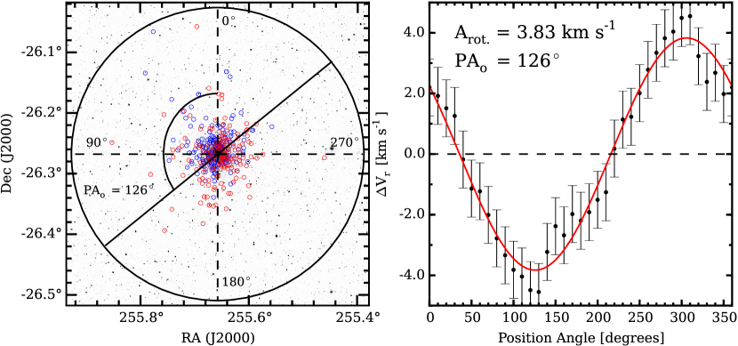
Figure 4.— Left: the sky coordinates of member stars with heliocentric radial velocities lower (blue) and higher (red) than the cluster average are superimposed on a 2MASS J–band image. The solid black line bisecting the cluster illustrates the position angle of the rotation axis (PA_o), which is measured by rotating the solid black line east through west and finding the maximum difference in heliocentric radial velocity on each side. Right: the average heliocentric radial velocity difference for position angles measured in 10$\arcdeg$ increments. The solid red line indicates the best–fit sinusoidal function to the data. See text for details.

For NGC 6273, we find a clear rotation signature with A_rot. = 3.83 $\pm$ 0.12 km s^-1 and PA_o = 126$\arcdeg$ $\pm$ 2$\arcdeg$. We calculated the rotation profile using various angular bin sizes and found that while A_rot. only varied by a few tenths of a km s^-1 the PA_o value could change by $\sim$15$\arcdeg$. Therefore, we follow Bellazzini et al. (2012) and have adopted the conservative 1$\sigma$ uncertainties of $\pm$0.5 km s^-1 for A_rot. and $\pm$30$\arcdeg$ for PA_o. Compared to the large globular cluster samples presented in Bellazzini et al. (2012), Kimmig et al. (2015), and Lardo et al. (2015), NGC 6273 exhibits relatively strong rotation. NGC 6273’s large A_rot. value is consistent with other clusters having similar metallicity and mass (e.g., $\omega$ Cen; see Figures 11 and 19 in Bellazzini et al. 2012 and Lardo et al. 2015, respectively).

In Figure 5, we also investigated the change in velocity dispersion as a function of the projected radial distance from the cluster center. As expected, we find that the velocity dispersion decreases from at least 10 km s^-1 inside 1$\arcmin$ to less than 5 km s^-1 outside 5$\arcmin$. We also estimated the cluster’s central velocity dispersion ($\sigma$_o) using simple Plummer models (Plummer 1911) of the form:

$$\sigma^{2}(r)=\frac{\sigma_{o}^{2}}{\sqrt{1+(\frac{r}{r_{h}})^{2}}},$$ (2)

where r_h is the Plummer scale radius. We fit two models: (1) one with both $\sigma$_o and r_h varied as free parameters and (2) one with $\sigma$_o varied as a free parameter and r_h held fixed. For the latter case, we assumed the half–light radius was approximately equal to the half–mass radius and adopted a half–light radius of 1.32$\arcmin$ (Harris 1996; 2010 revision). The resulting fit provided $\sigma$_o = 10.98 $\pm$ 0.40 km s^-1. For the former case, we found $\sigma$_o = 10.35 $\pm$ 0.69 km s^-1 and r_h = 1.67$\arcmin$ $\pm$ 0.41$\arcmin$.

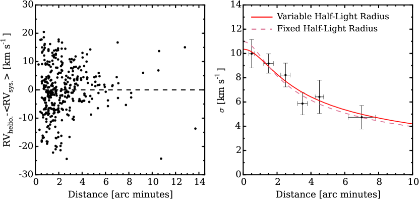
Figure 5.— Left: the radial velocity difference between each star and the cluster average is plotted as a function of the projected distance from the cluster center. Right: the velocity dispersion for various radial bins is plotted as a function of the projected distance from the cluster center. Inside 5$\arcmin$, the data are binned into 1$\arcmin$ bins, and the last bin includes all member stars with projected radial distances between 5–8.5$\arcmin$. The outer bin is shown for context but was not included in the fitting process. The solid red line shows the best–fit Plummer model when the central velocity dispersion and half–light radius are allowed to vary. The dashed light red line shows the best–fit Plummer model when the half–light radius is held fixed. See text for details.

However, we regard these values as lower limits of the true central velocity dispersion because the measured velocity dispersion for the bin closest to the cluster core is sensitive to the adopted bin size. For example, when the first bin contains stars with projected radial distances of 0.2–1.0$\arcmin$, as is done in Figure 5, the dispersion is $\sim$10 km s^-1, but if we change the range to 0.2–0.7$\arcmin$ then the dispersion increases to $\sim$12 km s^-1. Furthermore, a simple Plummer model assumes spherical symmetry, but NGC 6273 is relatively elliptical in shape (White & Shawl 1987; Chen & Chen 2010). Additional velocity measurements inside $\sim$0.2–0.5$\arcmin$ and the application of more sophisticated models are likely to find a true $\sigma$_o $>$ 12 km s^-1. We estimate that the cluster’s true A_rot./$\sigma$_o ratio is $\sim$0.30–0.35, which is typical for massive elliptical metal–poor globular clusters (e.g., see Bellazzini et al. 2012; Kacharov et al. 2014; Kimmig et al. 2015; Lardo et al. 2015).

4. SPECTROSCOPIC ANALYSIS

4.1. Model Atmospheres

The model atmosphere parameters effective temperature (T_eff), surface gravity (log(g)), metallicity ([Fe/H]), and microturbulence ($\xi$_mic.) were determined spectroscopically for all radial velocity member stars observed with the Bulge$\_$GC1 setup. A spectroscopic determination of especially T_eff and log(g) is preferred over photometric measurements for NGC 6273 because of the cluster’s large and variable reddening (see Section 2.3). We followed the general analysis procedures outlined in Johnson et al. (2015a), which includes use of the 1D local thermodynamic equilibrium (LTE) line analysis code MOOG (Sneden 1973; 2014 version). In particular, we solved for T_eff by enforcing excitation equilibrium with the Fe I lines and solved for surface gravity by adjusting log(g) until the Fe I and Fe II lines provided the same abundance. In the few instances where only Fe I could be measured, we assigned stars a log(g) value that was compatible with other cluster members of similar temperature and metallicity. Microturbulence was measured by adjusting $\xi$_mic. until the derived log $\epsilon$(Fe I) abundance was independent of line strength. Finally, the metallicity of each model was set as the average of [Fe I/H] and [Fe II/H].

In order to generate the models, we interpolated within the available grid of ATLAS9 model atmospheres (Castelli & Kurucz 2004). For most stars, we used the $\alpha$–enhanced models in order to compensate for the difference between [Fe/H] and [M/H]. However, a small number of stars in our sample have [$\alpha$/Fe] $\sim$ 0, and for those stars we used the scaled–solar models. For every star, we started with a base–line model of T_eff = 4500 K, log(g) = 1.20 cgs, [Fe/H] = –1.60 dex, and $\xi$_mic. = 1.70 km s^-1, and iteratively solved for all four parameters simultaneously.

Lind et al. (2012) showed that for some stars departures from LTE can have a significant impact on the model atmosphere parameters derived by spectroscopic methods. However, the impact on stars in the temperature, gravity, and metallicity regime probed here is likely to be small. Additionally, the relative effects due to departures from LTE should be mostly negligible within a small parameter space (e.g., Wang et al. 2016), and we have attempted to empirically cancel out large non–LTE and 3D model atmosphere deficiencies by performing a differential analysis relative to Arcturus. Therefore, we have not applied any non–LTE corrections to our data. We note also that Dupree et al. (2016) showed the addition of a chromosphere may alter the derived abundances for some elements. However, since we lack the spectral coverage necessary for constraining a chromospheric model, our model atmosphere parameters and abundances are based only on radiative/convective equilibrium models. The final model atmosphere parameters for all member stars derived from the Bulge$\_$GC1 data are provided in Table 4.

4.2. Equivalent Width and Spectrum Synthesis Measurements

The abundances of Si I, Ca I, Cr I, Fe I, Fe II, and Ni I were obtained by measuring the equivalent width (EW) of individual lines selected by Johnson et al. (2015a) to be relatively free of contamination from significant blends and residual telluric features. On average, the Si I, Ca I, Cr I, Fe I, Fe II, and Ni I abundances were based on the measurement of 2, 5, 2, 33, 4, and 4 absorption lines, respectively. However, we only measured the abundances of these elements from the Bulge$\_$GC1 spectra. We utilized the same EW measuring code, line list, and solar reference abundances described in Johnson et al. (2015a; see their Section 3.2 and their Table 2), and also used the same abfind driver in MOOG to calculate the final abundance ratios. The [Si I/Fe], [Ca I/Fe], [Cr I/Fe], [Fe I/H], [Fe II/H], and [Ni I/Fe] abundances for every cluster member observed in the Bulge$\_$GC1 setup are provided in Tables 5–6.

The abundances of Na I, Mg I, Al I, La II, and Eu II were obtained by using the synth driver in MOOG to fit synthetic spectra to the observations. The synthetic spectra were calculated using the line list developed for Johnson et al. (2015a), which is tuned to reproduce the Arcturus spectrum near the lines of interest and includes the updated CN line list from Sneden et al. (2014). We preferred to use spectrum synthesis rather than an EW analysis for these elements because their abundances are more sensitive to blending, contamination from other features, and/or broadening effects. For example, the Na and Al lines can have significant contamination from nearby atomic features and molecular CN, especially in the more metal–rich stars. Additionally, the Mg triplet near 6319 Å contains very weak lines, and the nearby continuum can be affected by a shallow but broad Ca I autoionization feature. The La and Eu lines are also relatively weak, but are further affected by hyperfine structure broadening. The Eu lines also contain a mixture of transitions from the ¹⁵¹Eu and ¹⁵³Eu isotopes, for which we assumed the ¹⁵¹Eu:¹⁵³Eu Solar System ratio of 47.8$\%$:52.2$\%$ (Lawler et al. 2001).

The final [Na/Fe], [Mg/Fe], [Al/Fe], [La/Fe], and [Eu/Fe] abundances derived for cluster members observed with the Bulge$\_$GC1 setup are provided in Tables 5–6. All atomic parameters and solar reference abundances are available in Johnson et al. (2015a; their Table 2).

4.3. Calcium Triplet Abundances

In addition to the [Fe/H] abundances derived from the EW measurements of individual Fe I and Fe II lines, we measured [Fe/H] in a larger sample of stars using the 8542 Å and 8662 Å CaT lines. These strong lines have been shown to be sensitive to a star’s metallicity and relatively insensitive to a star’s age or [$\alpha$/Fe] abundance, in a variety of environments (e.g., Armandroff & Da Costa 1991; Olszewski et al. 1991; Idiart et al. 1997; Rutledge et al. 1997; Cole et al. 2004; Carrera et al. 2007; Battaglia et al. 2008; Da Costa 2016b). Although several CaT–metallicity calibrations exist (e.g., Starkenburg et al. 2010; Saviane et al. 2012; Carrera et al. 2013; Vásquez et al. 2015), we followed the technique outlined in Yong et al. (2016) that utilizes the Mauro et al. (2014) calibration.

As noted by Yong et al. (2016), the Mauro et al. (2014) calibration has two significant advantages for NGC 6273: (1) the luminosity component of the calibration depends on a star’s K_S magnitude, rather than V magnitude, which is much less affected by differential reddening; and (2) the significantly flatter slope of the summed EW ($\Sigma$EW) versus K_S(HB)–K_S relation reduces the effects of photometric, distance, and reddening uncertainties on the derived [Fe/H] values. Additionally, we note that 2MASS provides uniform K_S photometry for our entire sample, but uniform V magnitudes are not yet available for all stars. However, since most CaT–metallicity relations may only be reliable down to the luminosity level of the HB (e.g., Da Costa et al. 2009), we did not determine CaT metallicities for stars fainter than the HB. This cut–off primarily affected the FLAMES CaT sample.

The Mauro et al. (2014) calibration requires a measurement of the summed 8542 Å and 8662 Å CaT EWs, defined as:

$$\Sigma EW=EW_{8542}+EW_{8662},$$ (3)

and the value K_S(HB)–K_S, where K_S(HB) is the magnitude of the horizontal branch. Following Yong et al. (2016), we have adopted K_S(HB) = 12.85 magnitudes (Valenti et al. 2007). The EWs for each line were fit using a function that is the sum, rather than the convolution, of a Gaussian and Lorentzian profile. Using Equation 7 and following Mauro et al. (2014), we adopted their relation,

$$\Sigma EW=-0.385[K_{S}(HB)-K_{S}]+W^{\prime},$$ (4)

to solve for the reduced equivalent width (W^′). The [Fe/H] values for each star were then determined using Equation 8 and the cubic calibration from Mauro et al. (2014) for the Carretta et al. (2009a) metallicity scale:

$$[Fe/H]=-4.61+1.842\langle{W}^{\prime}\rangle-0.4428\langle{W}^{\prime}\rangle^{2}+0.04517\langle{W}^{\prime}\rangle^{3}.$$ (5)

The individual EWs, $\Sigma$EW, and W^′ values for all NGC 6273 members are provided in Table 7.

A comparison between the observations of Yong et al. (2016) and our CaT data set revealed 27 stars in common. For this subset, the Yong et al. (2016) [Fe/H] values are on average 0.06 dex more metal–rich than ours, but the metallicities from both studies are well–correlated (see Figure 6). Similarly, we found 50 stars in our sample that were observed in both the CaT and Bulge$\_$GC1 setups, and a comparison of the derived [Fe/H] values is provided in Figure 6. The [Fe/H] measurements from both data sets are relatively well–correlated, but the CaT data are 0.12 dex more metal–rich, on average. Therefore, the final CaT–based [Fe/H] abundances provided in Table 7, and used throughout the rest of the paper, have been shifted by –0.12 dex in order to place the CaT and Bulge$\_$GC1 data sets on the same scale.

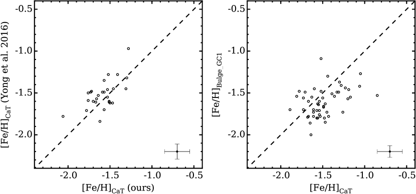
Figure 6.— Left: a comparison of the CaT [Fe/H] values derived in this work and Yong et al. (2016), for 27 stars in common. The dashed line indicates perfect agreement. Right: a comparison of the [Fe/H] values derived from the CaT and Bulge$\_$GC1 data sets of this work, for 50 stars in common. Note that in both panels our CaT [Fe/H] values are those derived from Equation 9 and have not yet been corrected to place the CaT [Fe/H] abundances on the Bulge$\_$GC1 [Fe/H] scale. Typical error bars are shown in the bottom right corner of each panel.

4.4. Internal Abundance Uncertainties

For the reasonably high S/N Bulge$\_$GC1 region spectra analyzed here, the dominant sources of internal abundance uncertainties are related to the line–to–line abundance scatter from uncertain log(gf) values, small profile fitting and/or continuum placement errors, and model atmosphere parameter uncertainties. The standard error of the mean provides a reasonable estimate of the abundance errors due to line list and profile fitting uncertainties, and for this data set we find a typical measurement uncertainty of 0.05 dex ($\sigma$ = 0.03 dex) in log $\epsilon$(X).

In order to estimate the uncertainties in T_eff and log(g), we provide a comparison of the spectroscopically derived parameters with those expected from Dartmouth isochrones (Dotter et al. 2008) with ages of 12 Gyr, [$\alpha$/Fe] = $+$0.4 dex, and [Fe/H] = –1.75, –1.50, and –1.20 dex in Figure 7. The isochrones with different [Fe/H] are included because of the metallicity spread detected in the cluster (Johnson et al. 2015a; Han et al. 2015; Yong et al. 2016; see also Section 5.1). Figure 7 shows that the derived temperature and surface gravity values are in good agreement with those predicted by the isochrones. Specifically, we find the average differences between the spectroscopic and isochrone temperature ($\Delta$T_eff) and surface gravity ($\Delta$log(g)) values to be –8 K and $+$0.01 cgs, respectively, and do not detect any significant trends as a function of temperature, gravity, or metallicity. The dispersions in $\Delta$T_eff and $\Delta$log(g) are found to be 92 K and 0.17 cgs, respectively. Therefore, we have adopted 100 K and 0.15 cgs as the typical model atmosphere uncertainties for T_eff and log(g). For the model atmosphere metallicity, we have adopted an uncertainty of 0.10 dex based on the combined measurement errors of [Fe I/H] and [Fe II/H]. Additionally, we estimate the typical $\xi$_mic. uncertainty to be 0.10 km s^-1 based on the scatter and fitting uncertainties present in plots of log $\epsilon$(Fe I) versus log(EW/$\lambda$).

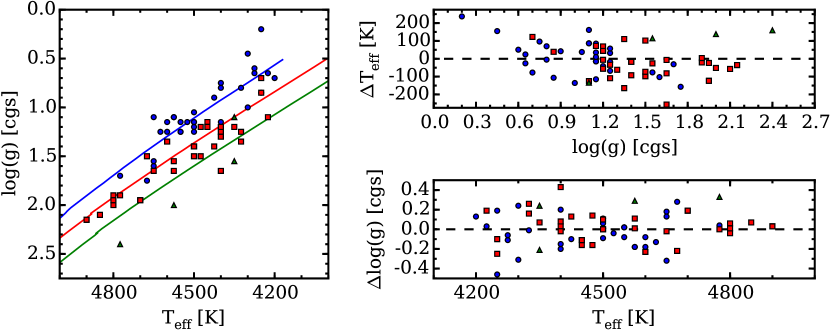
Figure 7.— The left panel shows the T_eff and log(g) values derived here and in Johnson et al. (2015) for the metal–poor ([Fe/H] $<$ –1.65; filled blue circles), metal–intermediate (–1.65 $<$ [Fe/H] $\leq$ –1.35; filled red boxes), and metal–rich ([Fe/H] $>$ –1.35; filled green triangles) populations, and compares the spectroscopic parameters with those predicted by Dartmouth isochrones (Dotter et al. 2008). The isochrones have an age of 12 Gyr, [$\alpha$/Fe] = 0.4 dex, and [Fe/H] = –1.75 (blue line), –1.50 (red line), and –1.20 dex (green line). The top right panel compares the differences between the spectroscopic and isochrone temperatures ($\Delta$T_eff) for a given surface gravity. Similarly, the bottom right panel compares the differences between the spectroscopic and isochrone surface gravities ($\Delta$log(g)) for a given temperature.

The abundance uncertainty values ($\Delta$[X/Fe] or $\Delta$[Fe/H]) were determined by rerunning MOOG and changing each model atmosphere parameter by the estimated uncertainties listed previously. Only one parameter was changed per run while the other values were held fixed. To speed up the analysis, we converted abundances to EWs for the elements measured by spectrum synthesis using the ewfind driver in MOOG. The total internal abundance uncertainties listed in Tables 5–6 were determined by adding the model atmosphere error terms, plus the random measurement uncertainties, in quadrature.

For the CaT data, we estimated the abundance uncertainties by analyzing the correlation between the 8542 Å and 8662 Å EWs. In other words, we used the strong correlation between EW₈₅₄₂ and EW₈₆₆₂ to predict the EW of each line based on the other one. The predicted EWs were then propagated through Equations 8–9, and the difference between these values and the [Fe/H] abundance given in Table 7 was taken as the measurement error. Using this method, we found an average $\Delta$[Fe/H] = 0.15 dex ($\sigma$ = 0.07 dex). We note that this value is similar to the fitting uncertainty of Equation 9 (Mauro et al. 2014). A typical [Fe/H] uncertainty of 0.15 dex is also similar to the 1$\sigma$ scatter (0.21 dex) between [Fe/H] values determined from the CaT and Bulge$\_$GC1 data.

5. RESULTS AND DISCUSSION

5.1. Metallicity Distribution

The color and CaT abundance spreads observed by Piotto et al. (1999) and Rutledge et al. (1997) provided some of the first evidence that NGC 6273 may host stars with different metallicities. More recently, high resolution spectroscopic measurements from Johnson et al. (2015a) showed that the cluster contains stars with [Fe/H] ranging from –1.80 to –1.30 dex, and also found that the cluster hosts at least two distinct populations separated in [Fe/H] by $\sim$0.25 dex. Similarly, Han et al. (2015) used narrow–band hk photometry to clearly show that the cluster’s sub–giant branch and RGB are split into two sequences with different compositions. Yong et al. (2016) also reported CaT metallicities ranging from [Fe/H] = –1.84 to –0.70 dex, further indicating the presence of a large metallicity spread in the cluster.

The Johnson et al. (2015a) and Yong et al. (2016) spectroscopic results are based on the analysis of only 18 and 44 RGB stars observed in the Bulge$\_$GC1 and CaT spectral regions, respectively. Therefore, we add here [Fe/H] measurements for 51 RGB members in the Bulge$\_$GC1 region and 191 RGB members in the CaT region (see Tables 4, 6, and 7). For the Bulge$\_$GC1 data, we find a full range of [Fe/H] = –2.00 to –1.09 dex, an average $\langle$[Fe/H]$\rangle$ = –1.61 dex, a dispersion ($\sigma$_[Fe/H]) of 0.18 dex, and an interquartile range (IQR) of 0.24 dex. Similarly, the CaT data exhibit a full range of [Fe/H] = –2.22 to –0.56 dex, an average $\langle$[Fe/H]$\rangle$ = –1.73 dex, $\sigma$_[Fe/H] = 0.24 dex, and an IQR of 0.27 dex. A comparison between the Bulge$\_$GC1 and CaT metallicity distributions is shown in Figure 8, and both data sets provide evidence that NGC 6273 harbors an intrinsic metallicity spread.

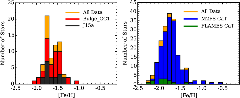
Figure 8.— The left and right panels compare the [Fe/H] distribution functions derived from data obtained with the Bulge$\_$GC1 and CaT spectrograph setups, respectively. For the left panel, the orange histogram represents the sum of the metallicities derived from this work and Johnson et al. (2015a). Similarly, in the right panel the orange histogram represents the sum of the M2FS and FLAMES CaT metallicities. All of the data are sampled with 0.10 dex [Fe/H] bins. Note the broad [Fe/H] range found in both data sets, and also the likely presence more than one distinct population in the Bulge$\_$GC1 data set. The [Fe/H] distributions in both panels only include stars that are radial velocity members.

Further examination of Figure 8 also indicates that NGC 6273 may host distinct populations with different [Fe/H], rather than just a broadened distribution. Specifically, Figure 8 suggests that at least three major components may exist: (1) a “metal–poor” population ([Fe/H] $\leq$ –1.65); (2) a “metal–intermediate” population (–1.65 $<$ [Fe/H] $\leq$ –1.35); and a “metal–rich” tail ([Fe/H] $>$ –1.35), and that these components constitute 46$\%$ $\pm$ 8$\%$, 48$\%$ $\pm$ 8$\%$, 6$\%$ $\pm$ 4$\%$ of our total Bulge$\_$GC1 data set, respectively. We find the average metallicities of the metal–poor, metal–intermediate, and metal–rich populations to be: $\langle$[Fe/H]$\rangle$ = –1.77 dex ($\sigma$ = 0.08 dex), $\langle$[Fe/H]$\rangle$ = –1.51 dex ($\sigma$ = 0.07 dex), and $\langle$[Fe/H]$\rangle$ = –1.22 dex ($\sigma$ = 0.09 dex), respectively. The clustering of stars near [Fe/H] = –1.75 and –1.50 is consistent with the [Fe/H] abundances and split RGB sequences derived by Johnson et al. (2015a) and Han et al. (2015), and the presence of a metal–rich tail extending up to at least [Fe/H] $\approx$ –1 matches the findings of Yong et al. (2016).

Figure 9 indicates that a radial metallicity gradient may exist in the cluster such that the metal–intermediate stars are more centrally concentrated than the metal–poor stars. Although the metal–rich stars observed with the Bulge$\_$GC1 setup all reside inside 3$\arcmin$ of the cluster center (see also Figure 3), the sample size is too small to draw any strong conclusions about this population’s radial distribution. For the two dominate populations, a difference in their radial distributions is only observed at projected distances $\gtrsim$ 1.5$\arcmin$ from the cluster center, and a two–sided Kolmogorov–Smirnov test indicates that we do not have enough evidence to reject the null hypothesis that the two data sets are drawn from the same radial distribution. However, we note that the radial range where the distributions may differ is within $\sim$1–3 half–mass radii, which is the region that Vesperini et al. (2013) estimate the local population mixtures may closely match the global ratios. Interestingly, if the radial segregation of stars with different metallicities is confirmed from larger sample sizes, then NGC 6273 would share a similar metallicity gradient morphology with $\omega$ Cen (e.g., Norris et al. 1996; Suntzeff & Kraft 1996; Rey et al. 2004; Bellini et al. 2009; Johnson & Pilachowski 2010). Such a gradient would contrast with NGC 1851 where Carretta et al. (2010b) found the metal–poor stars to be the most centrally concentrated.

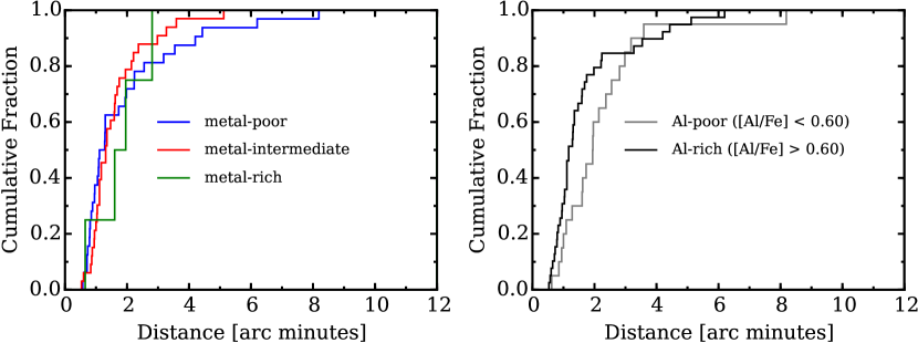
Figure 9.— Left: the cumulative distribution functions of the metal–poor (blue), metal–intermediate (red), and metal–rich (green) populations are shown as a function of the projected distance from the cluster center. Note the preferential central concentration of metal–intermediate, and possibly metal–rich, stars at distances $\gtrsim$ 1.5$\arcmin$. Right: a similar plot comparing the radial distributions of Al–poor (grey; “first generation”) and Al–rich (black; “second generation”) stars from all three major populations. Note the significant central concentration of Al–rich stars.

5.2. Additional Evidence of a Complex Metallicity Distribution

Spectroscopic observations have indicated that several clusters, including $\omega$ Cen (e.g., Norris & Da Costa 1995; Johnson & Pilachowski 2010; Marino et al. 2011a), NGC 5286 (Marino et al. 2015), M 2 (Yong et al. 2014), M 54 (Carretta et al. 2010a), Terzan 5 (Origlia et al. 2013; Massari et al. 2014), NGC 1851 (Yong & Grundahl 2008; Carretta et al. 2011; Lim et al. 2015), and M 22 (Pilachowski et al. 1982; Da Costa et al. 2009; Marino et al. 2009, 2011b), may host multiple populations with distinct [Fe/H] ratios. However, recent studies by Mucciarelli et al. (2015a) and Lardo et al. (2016) claim that at least some of these [Fe/H] spreads are spurious detections driven by a disparity between [Fe I/H] and [Fe II/H]. Similarly, Ivans et al. (2001), Lapenna et al. (2014), and Mucciarelli et al. (2015b) found that [Fe/H] determinations for RGB and AGB stars can differ systematically by $>$ 0.1 dex, and that mixing RGB and AGB stars in a sample can produce an artificial metallicity spread. A common thread connecting these issues is the method by which a star’s surface gravity is determined (spectroscopic versus photometric). Specifically, spectroscopic determinations may produce optimal log(g) values that correspond to masses which are systematically too low ($<$ 0.5 M_⊙ in many cases). Since we utilize a spectroscopic surface gravity method and find that NGC 6273 shares many chemical and morphological characteristics with clusters such as M 2 and M 22, for which intrinsic [Fe/H] spreads are contested, it is prudent to examine alternative lines of evidence that may support or refute NGC 6273 possessing an intrinsic metallicity spread.

Both spectroscopy and photometry unambiguously agree that $\omega$ Cen possesses discrete RGB populations with different [Fe/H], and in Figure 10 we directly compare the spectra of NGC 6273 and $\omega$ Cen stars that have physical parameters typical of those in the metal–poor, metal–intermediate, and metal–rich groups. The $\omega$ Cen temperature and gravity parameters were determined entirely from photometric methods (see Johnson & Pilachowski 2010), assuming masses of 0.8 M_⊙, and therefore should avoid the potential spectroscopic gravity problems noted above. As can be seen in Figure 10, the nearly identical Fe I and Fe II line profiles suggest that the NGC 6273 and $\omega$ Cen stars share similar compositions across a wide [Fe/H] range. We note also that the CaT [Fe/H] distribution shown in Figure 8 for NGC 6273 closely matches the extended metallicity distribution found in $\omega$ Cen (e.g., Norris et al. 1996; Suntzeff & Kraft 1996).

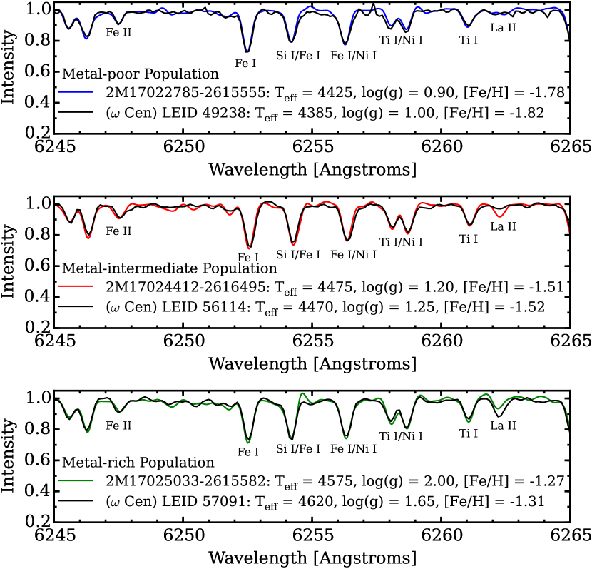
Figure 10.— This figure compares the spectra of stars in NGC 6273 and $\omega$ Cen (Johnson & Pilachowski 2010) that have similar T_eff, log(g), and [Fe/H]. The top, middle, and bottom panels show stars from the metal–poor, metal–intermediate, and metal–rich groups, respectively. In these panels, the colored spectra are from stars in NGC 6273 and the black spectra are from stars in $\omega$ Cen. The NGC 6273 M2FS spectra have been smoothed to match the resolution of the $\omega$ Cen Hydra spectra (R $\sim$ 18,000).

As shown in Figure 2, the broad color dispersion along the upper RGB provides some evidence that NGC 6273 may harbor an intrinsic metallicity spread. We investigate this further in Figure 11 by examining the upper RGB regions of the (F336W)_o versus (F336W–F555W)_o and (F555W)_o versus (F438W–F555W)_o color–magnitude diagrams and identifying the Bulge$\_$GC1 spectroscopic targets with different [Fe/H]. Both color–magnitude diagrams indicate that the two dominant metallicity groups tend to separate on the upper RGB. The (F336W)_o versus (F336W–F555W)_o plot in particular suggests that the brightest $\sim$ 0.5 magnitudes of the RGB–tip may split into at least two sequences with different [Fe/H], which is similar to the result found by Marino et al. (2015) for NGC 5286. However, the F336W and F438W filters, and by extension the F336W–F555W and F438W–F555W colors, can be sensitive to both a star’s overall metallicity and its C$+$N$+$O abundances. Therefore, the color–magnitude diagrams shown in Figure 11 are consistent with an intrinsic metallicity spread, but a detailed examination of the cluster’s CNO (and also He) abundances is required in order to fully confirm this result. Interestingly, the two metal–rich stars in Figure 11 are located at colors that are bluer than might be expected from their metallicities alone. We note that similar observations have been found for the equivalent “s–poor/Fe–rich” stars in NGC 5286 (Marino et al. 2015) and M 2 (Yong et al. 2014). The bluer colors for these stars may reflect lower atmospheric opacities driven by different light element compositions and perhaps lower [$\alpha$/Fe] ratios, at least for NGC 6273.

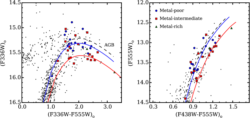
Figure 11.— The left and right panels compare the upper RGB and AGB regions of NGC 6273 using combinations of the dereddened F336W, F438W, and F555W bands. The Bulge$\_$GC1 observations that overlap with the WFC3 field–of–view are distinguished by metallicity using the same criteria, colors, and symbols as those in Figure 7. The two panels include Dartmouth isochrones with ages of 12 Gyr, [$\alpha$/Fe] = 0.4 dex, distances of 9 kpc, and [Fe/H] = –1.75 (blue lines) and –1.50 (red lines) dex, which correspond to the metallicities of the two dominant populations. The dashed black lines separate the RGB and AGB stars. The bluer colors of the most metal–rich stars (green triangles) suggest that these stars may have different He, C, N, and O abundances than the metal–intermediate population and/or may be higher metallicity AGB stars.

Figure 11 also shows that very few of our Bulge$\_$GC1 targets are on the AGB, indicating that the measured metallicity spread is not caused by systematic differences in the RGB and AGB abundance scales. In fact, the few AGB stars in our sample appear to belong to both the metal–poor and metal–intermediate populations, and the two metal–rich stars could also belong to a more metal–rich AGB sequence. Therefore, we regard the combined evidence of separate subgiant and RGB sequences observed by Han et al. (2015) with the hk filter, the RGB color dispersions seen in Figures 2 and 11 here, the large metallicity spreads detected previously by Johnson et al. (2015a) and Yong et al. (2016), and the spectroscopic data presented here as strong evidence that NGC 6273 possesses an intrinsic metallicity spread.

5.3. Light and Heavy Element Chemical Abundance Patterns

5.3.1 Alpha Element Abundances

The $\alpha$ elements Mg, Si, and Ca are largely produced during hydrostatic and explosive carbon, neon, and oxygen burning in massive stars (e.g., Woosley & Weaver 1995). In environments where chemical enrichment has been dominated by the products of core–collapse supernovae (SNe), one tends to find stars with [$\alpha$/Fe] abundances that are enhanced by about a factor of 2–3 over the solar ratio (e.g., see review by McWilliam 1997). In contrast, longer enrichment time scales may produce stars with lower [$\alpha$/Fe] ratios as Type Ia SNe begin to contribute larger amounts of Fe–peak elements than $\alpha$ elements (Tinsley 1979).

As can be clearly seen in Gratton et al. (2004; their Figure 4), nearly all Galactic globular clusters have [$\alpha$/Fe] $\sim$ 0.2–0.4 dex. Furthermore, the star–to–star scatter of [$\alpha$/Fe] within a given cluster is typically $<$ 0.1 dex, which suggests that the products of core–collapse SNe were well–mixed. Only a small number of clusters, such as Ruprecht 106, Terzan 7, and Palomar 12, are known to have abnormally low [$\alpha$/Fe] ratios (e.g., Pritzl et al. 2005), and all three of these clusters are thought to have extragalactic/accretion origins (e.g., Cohen 2004; Law & Majewski 2010; Villanova et al. 2013). Therefore, one does not normally expect to find stars with enhanced and depleted [$\alpha$/Fe] ratios within a single globular cluster, beyond the well–known proton–capture nucleosynthesis variations (see Section 5.3.2). In fact, only the massive iron–complex clusters $\omega$ Cen, NGC 6273, M 54, M 2, and Terzan 5 show any evidence of hosting stars with different [$\alpha$/Fe] ratios (Pancino et al. 2002; Origlia et al. 2003, 2011, 2013; Carretta et al. 2010a; Johnson & Pilachowski 2010; Yong et al. 2014; Johnson et al. 2015a).

Figure 12 and Table 8 show the [Mg/Fe], [Si/Fe], [Ca/Fe], and averaged [$\alpha$/Fe] patterns of NGC 6273’s various populations. In agreement with Johnson et al. (2015a), we find that most stars in NGC 6273 have elevated $\alpha$ element abundances, but that the average [Mg/Fe] and [Si/Fe] ratios may decrease slightly as a function of increasing metallicity. The [Si/Fe] abundances in particular may show additional substructure, and we find some evidence that the average [Si/Fe] abundances of the “$\alpha$–enhanced” metal–intermediate stars may be lower than those of the metal–poor and metal–rich groups. We note that a similar change in the [Si/Fe] abundances with [Fe/H] has been observed in $\omega$ Cen (Johnson & Pilachowski 2010), which suggests that this trend could be the signature of a particular self–enrichment mode in massive clusters. However, the [Ca/Fe] abundances show no significant trends as a function of [Fe/H], and the typical dispersion within each sub–population is $\sim$0.1 dex.

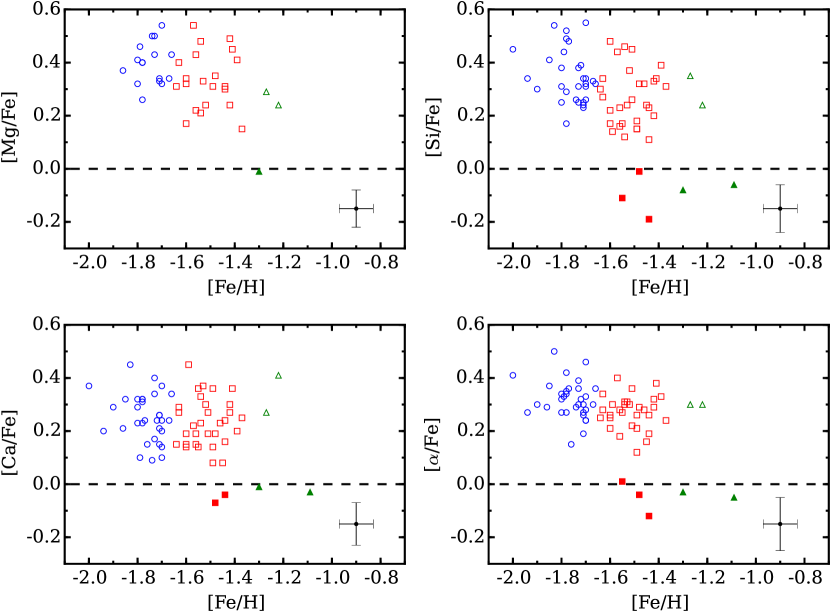
Figure 12.— The [Mg/Fe], [Si/Fe], [Ca/Fe], and [$\alpha$/Fe] ratios for NGC 6273 stars observed in this work and Johnson et al. (2015a) are plotted as a function of [Fe/H]. The open blue circles, red boxes, and green triangles designate stars belonging to the metal–poor, metal–intermediate, and metal–rich populations, respectively. The filled symbols indicate stars that have low [Mg/Fe], [Si/Fe], [Ca/Fe], and [$\alpha$/Fe] abundances. The dashed black lines indicate the solar [X/Fe] ratios, and the [$\alpha$/Fe] abundances represent the average values of [Mg/Fe], [Si/Fe], and [Ca/Fe] measured in each star. Typical error bars are included in the bottom right corner of each plot.

In a previous analysis, Johnson et al. (2015a) discovered that the most metal–rich star in their sample exhibited low [X/Fe] ratios for several species, including the $\alpha$ elements. The new data presented here indicate that not all metal–rich stars have low [$\alpha$/Fe], but we find at least five “low–$\alpha$” stars that have approximately solar [Mg/Fe], [Si/Fe], and [Ca/Fe] abundances. As can be seen in Figure 12, all five low–$\alpha$ stars have [Fe/H] $>$ –1.5 dex. Additionally, the specific frequency of low–$\alpha$ stars increases with metallicity such that these stars constitute 9$\%$ (3/33) of the metal–intermediate population and 50$\%$ (2/4) of the metal–rich population. However, we caution that the measured specific frequency values are likely affected by small number statistics and should be confirmed with additional observations.

Although we noted above that $\omega$ Cen, M 54, M 2, and Terzan 5 also contain stars with higher [Fe/H] and lower [$\alpha$/Fe], none of these clusters exactly matches the pattern of NGC 6273. For example, the $\alpha$–poor stars in M 2 and Terzan 5 are exclusively found in the most metal–rich populations, but neither cluster appears to contain $\alpha$–enhanced and $\alpha$–poor stars at the same metallicity. Although Johnson & Pilachowski (2010; see their Figure 10) found several stars with high and low [Si/Fe] and [Ca/Fe] abundances across a broad range of [Fe/H] in $\omega$ Cen, follow–up observations are required to confirm that this pattern matches what is found in NGC 6273.

Interestingly, the M 54 cluster and Sagittarius nuclear field star system may provide the closest example to what is observed in NGC 6273 (see Carretta et al. 2010a). In this system, the metal–poor cluster M 54 contains a metallicity spread but only $\alpha$–enhanced stars. In contrast, the surrounding galaxy field stars are generally more metal–rich and have lower [$\alpha$/Fe]. Therefore, if NGC 6273 formed in the core of a system similar to the Sagittarius dwarf galaxy, then the cluster may have been able to accrete a small number of metal–rich, $\alpha$–poor field stars from its progenitor population. Alternatively, the low–$\alpha$ stars in NGC 6273 may have been preferentially polluted by the ejecta of Type Ia SNe, perhaps in a scenario similar to that discussed in D’Antona et al. (2016). However, such a scenario would have to be able to produce low–$\alpha$ stars with different [Fe/H] but otherwise similar compositions (see Sections 5.3.2 and 5.3.3), and may even have to occur multiple times in clusters like NGC 6273.

5.3.2 Light Element Abundances

As mentioned in Section 1, globular clusters show clear light element abundance variations that extend beyond the effects of first dredge–up and are a result of high temperature ($>$ 40 MK; Langer et al. 1993, 1997; Prantzos et al. 2007) proton–capture burning. Since these effects are observed in main–sequence and evolved RGB stars (e.g., Gratton et al. 2001), we know that the gas from which present day cluster stars formed was polluted by a previous generation of more massive stars. Although the exact nucleosynthesis sources remain a mystery, the observed effects include anti–correlations among the element pairs C–N, O–N, O–Na, O–Al, and Mg–Al and correlations of C–O, N–Na, and Na–Al (e.g., Sneden et al. 2004). He enhancements are also likely found in stars with low O/Mg and high Na/Al (e.g., Bragaglia 2010a,b; Dupree et al. 2011). For this paper, we adopt the common nomenclature that “first generation” stars are those with compositions similar to metal–poor halo field stars (i.e., lower He, N, Na, and Al abundances; higher C, O, and Mg abundances) and “second generation” stars are those with enhanced He, N, Na, and Al abundances and depleted C, O, and possibly Mg abundances.

The Mg–Al anti–correlation is only found in a handful of the most massive clusters, but may be particularly useful for identifying discrete populations (e.g., Carretta 2014, 2015). Since the full Mg–Al cycle is activated at a higher temperature than the O–N and Ne–Na cycles, the presence (or not) of a Mg–Al anti–correlation provides important insight into the burning temperatures achieved by the pollution sources. Similarly, a few of the most massive clusters also exhibit abundance variations that extend to elements as heavy as Si, K, and Sc, which is likely a byproduct of even higher temperature proton–capture burning (Yong et al. 2005; Carretta et al. 2009b, 2013, 2014; Johnson & Pilachowski 2010; Cohen & Kirby 2012; Mucciarelli et al. 2012, 2015c; Ventura et al. 2012; Carretta 2015; Roederer & Thompson 2015). Notably, many of these clusters share similar properties with NGC 6273, such as extended blue HBs.

In Figure 13 and Table 8, we compare the [Na/Fe], [Mg/Fe], [Al/Fe], and [$\alpha$/Fe] abundances of the three different metallicity groups in NGC 6273. Similar to the results of Johnson et al. (2015a), we find that both [Na/Fe] and [Al/Fe] vary by about factors of 5 and 10, respectively, and that clear Na–Al correlations are independently present in the metal–poor, metal–intermediate, and metal–rich populations. Therefore, NGC 6273 shares a common feature observed in other iron–complex clusters: each population with a unique metallicity was able to generate its own independent spread of light element abundances that closely resembles the patterns exhibited by monometallic clusters.

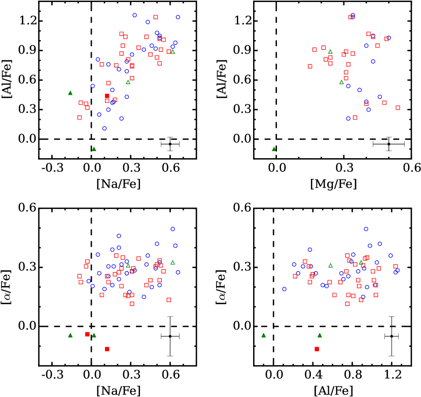
Figure 13.— Top: these panels show the NGC 6273 [Al/Fe] abundances from this work and Johnson et al. (2015a) plotted as a function of [Na/Fe] (left) and [Mg/Fe] (right). A clear Na–Al correlation exists for all three metallicity groups, but a Mg–Al anti–correlation may only be present in the metal–intermediate and metal–rich populations. The colors and symbols are the same as those in Figure 12. Bottom: these panels plot the [$\alpha$/Fe] ratios as a function of [Na/Fe] (left) and [Al/Fe] (right). Note that all of the “low–$\alpha$” stars have low [Na/Fe] and [Al/Fe] abundances.

The Na–Al correlation in Figure 13 shows a paucity of stars near [Al/Fe] $\sim$ 0.6 dex. If we adopt this cut–off as the discriminator between first and second generation stars, then we find that approximately two–thirds of the cluster stars can be classified as second generation stars. The metal–poor and metal–intermediate populations each favor second generation stars with first:second generation ratios of 35$\%$:65$\%$ and 28$\%$:72$\%$, respectively. On the other hand, the metal–rich population has a ratio of 75$\%$:25$\%$, but this measurement is based on only 4 stars. Therefore, the numerical dominance of second generation stars in NGC 6273 fits a common trend observed in many Galactic globular clusters (e.g., Carretta et al. 2009a, see their Figure 10). Similarly, Figure 9 shows that the second generation stars in NGC 6273 are more centrally concentrated than the first generation stars, which again matches a pattern observed in many iron–complex and monometallic clusters (e.g., Lardo et al. 2011). We note also that an additional paucity of stars may be present near [Na/Fe] $\sim$ 0.35 dex, which may further distinguish the most Na/Al–rich stars. These stars, which constitute $\sim$ 33$\%$ of our sample, are likely equivalent to the “extreme” population found by Carretta et al. (2009a) in several clusters, the “E” population of NGC 2808 (Milone et al. 2015b), and the faint sub–giant branch stars of 47 Tuc (Marino et al. 2016). We note that a similarly high fraction of very Na/Al–rich stars is also found in $\omega$ Cen (Johnson & Pilachowski 2010; Marino et al. 2011) and M 54 (Carretta et al. 2010a).

For [Mg/Fe] and [Al/Fe], Figure 13 shows that the behavior of the element pair may change for stars of different metallicity in NGC 6273. The metal–poor component shows no correlation between [Mg/Fe] and [Al/Fe], but the metal–intermediate population shows evidence of a Mg–Al anti–correlation for stars with [Al/Fe] $<$ 1.0 dex. A similar Mg–Al anti–correlation may also be present for the metal–rich stars, but the sample size (4 stars) is too small to draw any clear conclusions. Since ²⁴Mg is only significantly depleted at temperatures $\gtrsim$ 65 MK (e.g., see Prantzos et al. 2007; their Figure 2), the different Mg–Al relations for the metal–poor and metal–intermediate stars suggest that the gas from which each population’s second generation stars formed was processed at different temperatures. However, we did not find any residual correlations between Mg or Al and the heavier elements like Si, which indicates that the pollution source(s) responsible for the Mg–Al anti–correlation in NGC 6273 likely did not reach temperatures high enough to significantly activate the ²⁷Al(p,$\gamma$)²⁸Si reaction related to the Mg–Al chain.

An examination of Mg–Al trends in the iron–complex clusters $\omega$ Cen, M 54, M 2, M 22, NGC 1851, and NGC 5286 revealed that only $\omega$ Cen (Norris & Da Costa 1995; Smith et al. 2000; Da Costa et al. 2013), M 54 (Carretta et al. 2010a), and NGC 1851 (Carretta et al. 2011, 2012) exhibit evidence of Mg–Al anti–correlations. Unlike NGC 6273, none of these clusters show evidence that the presence of a Mg–Al anti–correlation depends on a population’s metallicity. However, we note that in $\omega$ Cen the metal–intermediate and metal–rich stars exhibit clear changes in their light element patterns (e.g., Norris & Da Costa 1995; Johnson & Pilachowski 2010; Marino et al. 2011). For example, the very O–poor/Na–rich stars that dominate by number at higher metallicity are not found at [Fe/H] $\lesssim$ –1.8, and O and Na are actually correlated in the most metal–rich stars. Additionally, for M 54 Carretta et al. (2010a) found that the light element variations are more extended for the metal–rich stars than the metal–poor population. Therefore, NGC 6273, $\omega$ Cen, and M 54 provide evidence that a cluster’s enrichment signature can change with time, and that multiple pollution sources may be able to produce chemical patterns that are similar for some element pairs (e.g., Na–Al) but not others (e.g., Mg–Al).

Interestingly, Figure 13 shows that the metal–intermediate stars with [Al/Fe] $>$ 1.0 dex have [Mg/Fe] $\sim$ 0.4 dex, rather than the [Mg/Fe] $\sim$ 0.0 dex abundances that might be expected. The reason for this discrepancy is not immediately clear, but we note that many similar metallicity clusters have stars with [Mg/Fe] $\sim$ 0.4 dex and [Al/Fe] $\sim$ 1.0 dex (e.g., Carretta et al. 2009b; see their Figure 6). Additionally, we note that Norris & Da Costa (1995) found that intermediate metallicity stars in $\omega$ Cen could have [Al/Fe] $>$ 1.0 dex but [Mg/Fe] could range from about 0.6 dex (no Mg–Al anti–correlation) to 0.0 dex (clear Mg–Al anti–correlation; see also Carretta et al. 2010a, their Figure 18). In this context, an examination of the ²⁴Mg, ²⁵Mg, and ²⁶Mg abundances in NGC 6273, similar to the analysis of Da Costa et al. (2013) in $\omega$ Cen, could be particularly illuminating. However, we also caution that the 6319 Å Mg I lines used here are relatively weak, especially in stars with intrinsically low [Mg/Fe], so the exact shape of the Mg–Al anti–correlation should be confirmed with additional analyses.

Finally, we note that all of the low–$\alpha$ stars have [Na/Fe] and [Al/Fe] compositions that are consistent with those of first generation stars. Although the sample size of low–$\alpha$ stars is small, a simulation of 10⁵ random draws from our $\alpha$–enhanced population indicated that there is only about a 0.05$\%$ chance that we would randomly draw 5 stars that have [Na/Fe] $<$ 0.25 dex and [Al/Fe] $<$ 0.50 dex. Therefore, we speculate that the low–$\alpha$ population may have been unable to form second generation stars. The pattern of low [Na/Fe] and [Al/Fe] abundances in the low–$\alpha$ stars of NGC 6273 mirrors the composition differences found by Carretta et al. (2010a) when comparing the M 54 cluster and Sagittarius galaxy field stars. The similar composition patterns of the low–$\alpha$ stars in NGC 6273 and the Sagittarius field stars strengthens the idea that NGC 6273 may have accreted its low–$\alpha$ stars from a surrounding field population that was once part of a now dispersed dwarf galaxy.

5.3.3 RGB versus AGB Abundance Patterns

As noted by Gratton et al. (2010) and many previous authors (e.g., Mallia 1978; Norris et al. 1981; Suntzeff 1981; Smith & Norris 1993; Pilachowski et al. 1996a; Ivans et al. 1999; Sneden et al. 2000), some globular clusters may contain RGB and AGB populations with different light element abundances. Specifically, RGB stars that evolve onto the HB with masses $\lesssim$ 0.55 M_⊙, presumably those with the highest He, N, Na, and Al abundances and lowest C, O, and Mg abundances, may not ascend the AGB and instead end their lives as AGB–manqué stars (e.g., Greggio & Renzini 1990). As a result, we expect to find that the light element abundance distributions of AGB stars should exhibit a paucity of second generation stars when compared to the RGB ratios.

Renewed interest in this field has produced somewhat conflicting results with the missing second generation fraction ranging from 100$\%$ (Campbell et al. 2013; MacLean et al. 2016) to only a few percent (Johnson & Pilachowski 2012; García–Hernández et al. 2015; Johnson et al. 2015b; Lapenna et al. 2016; Wang et al. 2016). However, the growing consensus is that only the most extreme second generation stars probably fail to ascend the AGB.

Since Figure 14 shows that NGC 6273 contains a very extended blue HB, and that $\sim$30$\%$ of the cluster’s HB stars have masses $\lesssim$ 0.55 M_⊙, we investigate here whether any second generation stars may have failed to ascend the AGB. We restrict the comparison to only the targets shown in Figure 11 since these are the only stars in our sample that can be reliably assigned to either the RGB or AGB sequences. Although the sample sizes are small (9 AGB; 28 RGB), we find similar first:second generation ratios of 24$\%$:76$\%$ and 14$\%$:86$\%$ for the RGB and AGB samples, respectively. However, further inspection of the [Na/Fe] and [Al/Fe] distributions in Figure 15 reveals that the AGB sample does not contain stars with [Na/Fe] $>$ 0.5 dex nor [Al/Fe] $>$ 1.0 dex. In other words, only the most Na/Al–rich, and presumably He–enhanced, stars may have failed to ascend the AGB.

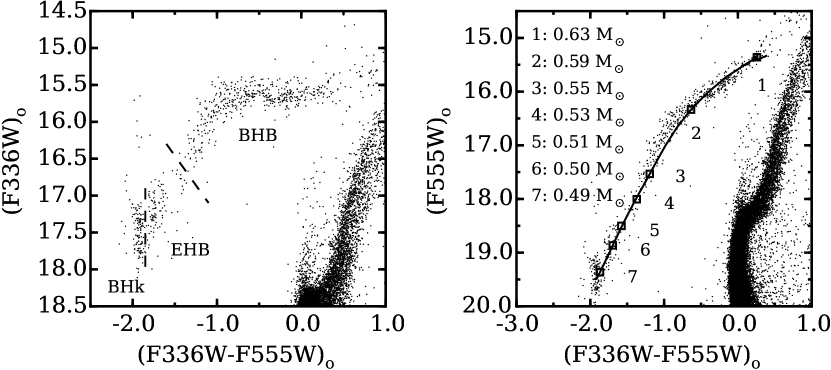
Figure 14.— left: an (F336W)_o versus (F336W–F555W)_o color–magnitude diagram is shown for the HB region. The black dashed lines approximately separate the blue HB (BHB), extreme HB (EHB), and blue hook (BHk) stellar populations. Note that the EHB may be composed of at least three subgroups that each span $\sim$0.5 magnitudes in (F336W)_o but $\lesssim$ 0.05–0.10 magnitudes in (F336W–F555W)_o color. A similarly small color spread is exhibited by the BHk stars as well. The small color ranges suggest mass ranges of $\lesssim$ 0.01 M_⊙ (e.g., see also Sosin et al. 1997; Momany et al. 2004). right: a similar (F555W)_o versus (F336W–F555W)_o color–magnitude diagram is shown that includes a 12 Gyr, $\alpha$–enhanced BASTI (Pietrinferni et al. 2006) isochrone of [Fe/H] = –1.62 (solid black line). The isochrone assumes a cluster distance of 9 kpc and has been shifted by –0.12 magnitudes in color in order to fit the red end of the blue HB. The open black boxes labeled 1–7 correspond to temperatures of 8,000 K, 11,500 K, 16,675 K, 20,000 K, 22,500 K, 25,800 K, and 32,000 K, respectively.

It is possible that the paucity of extreme Na/Al–rich AGB stars is a product of our small sample size. To investigate this, we performed 10⁵ random draws of an equivalent AGB sample from the RGB distribution, and we found about a 7$\%$ chance that the missing Na/Al–rich AGB stars could be due to the small sample size. Interestingly, the missing Na/Al–rich AGB stars account for $\sim$30$\%$ of the RGB sample, which is comparable to the fraction of extreme HB and blue hook stars found on the HB (see Figure 14 and Section 5.4). Therefore, we conclude that the NGC 6273 RGB stars with [Na/Fe] $>$ 0.5 dex and [Al/Fe] $>$ 1.0 dex likely evolve to become extreme HB or blue hook stars and fail to ascend the AGB.

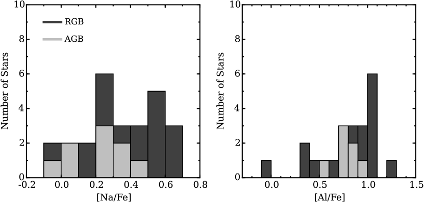
Figure 15.— The left and right panels compare the [Na/Fe] and [Al/Fe] distributions of the RGB (dark grey) and AGB (light grey) populations seen in Figure 11. Note that the AGB stars span a smaller range in both [Na/Fe] and [Al/Fe], and that no AGB stars were observed to have [Na/Fe] $>$ 0.50 dex and [Al/Fe] $>$ 1.0 dex.

5.3.4 Fe–Peak Element Abundances

The Fe–peak elements Cr and Ni are largely produced in the late burning stages of massive stars, but include some production by Type Ia SNe as well (e.g., Timmes et al. 1995). Within a single globular cluster, the star–to–star scatter in [Ni/Fe] and [Cr/Fe] is typically $\lesssim$ 0.1 dex (e.g., Gratton et al. 2004; see their Figure 2). Similarly, the average [Cr/Fe] and [Ni/Fe] ratios are about solar across the entire metallicity range spanned by clusters in the Galaxy.

In Figure 16 and Table 8, we show the abundance patterns of [Cr/Fe] and [Ni/Fe] for NGC 6273. Overall, we find $\langle$[Cr/Fe]$\rangle$ = 0.01 dex ($\sigma$ = 0.12 dex) and $\langle$[Ni/Fe]$\rangle$ = –0.05 dex ($\sigma$ = 0.11 dex), which is in agreement with Johnson et al. (2015a). An examination of Figure 16 shows that the metal–poor, metal–intermediate, and metal–rich stars all exhibit nearly identical [Cr/Fe] and [Ni/Fe] abundances and dispersions. However, we note that several (but not all) of the low–$\alpha$ stars have [Cr,Ni/Fe] $\lesssim$ –0.2 dex, similar to what is found in some clusters associated with the Sagittarius dwarf galaxy. A detailed examination of key Fe–peak elements that are sensitive to nucleosynthesis processes operating in different environments, such as Mn, Co, Zn, and Cu (e.g., Nomoto et al. 2006), may provide additional insight into whether the stars with low [$\alpha$/Fe], [Cr/Fe], and [Ni/Fe] have similar origins.

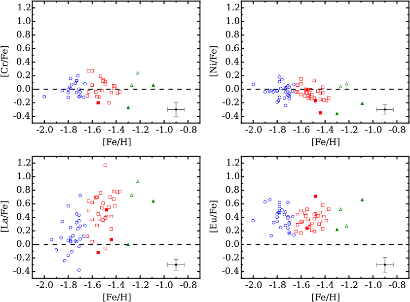
Figure 16.— The [Cr/Fe], [Ni/Fe], [La/Fe], and [Eu/Fe] abundances are plotted as a function of [Fe/H] for all three major populations in NGC 6273. The colors and symbols are the same as those in Figure 12.

5.3.5 Neutron–Capture Element Abundances

Most of the stable isotopes heavier than the Fe–peak are produced either by the r–process over short time scales or by the s–process over much longer time scales (e.g., see review by Sneden et al. 2008). As a result, old globular clusters tend to have heavy element compositions that are dominated by r–process nucleosynthesis, which is evidenced by their characteristically low [La/Eu] ratios (e.g., see Gratton et al. 2004; their Figure 6). Although the Galactic globular cluster system exhibits a trend of increasing s–process contributions at higher [Fe/H] (e.g., James et al. 2004), a small number of clusters, such as M4 (e.g., Ivans et al. 1999), deviate from this trend and exhibit significantly higher [La/Eu] ratios. In these clusters, the gas from which their stars formed likely experienced additional, but uniform, pollution from a previous generation of $\sim$1.5–4 M_⊙ AGB stars (e.g., Busso et al. 1999).

As mentioned in Section 1, one of the “chemical tags” of iron–complex clusters is that they exhibit clear correlations between [Fe/H] and the products of s–process enrichment. All iron–complex clusters for which the heavy elements have been measured contain populations of Fe/s–poor and Fe/s–rich stars with similar Ba and La enhancements (Marino et al. 2015; Johnson et al. 2015a). As a result, merger scenarios seem unlikely for every case because each cluster would have had to form from the coalescence of populations with nearly identical Fe/s–poor and Fe/s–rich compositions (but see also Gavagnin et al. 2016). Instead, we regard the combination of [Fe/H] and s–process enhancements as a sign that iron–complex clusters were able to sustain extended star formation and self–enrichment, and that the time frame was long enough for low and intermediate mass AGB stars to contribute to the composition of the more metal–rich stars.

Figure 16 and Table 8 show a clear increase in [La/Fe] with [Fe/H] for NGC 6273, in agreement with the results of Johnson et al. (2015a). Therefore, we confirm that NGC 6273 possesses the same s–process enrichment profiles as other iron–complex clusters. We also find for Eu that the cluster average is about [Eu/Fe] = 0.4 dex, regardless of a star’s metallicity. This suggests that massive stars were largely responsible for the increase in [Fe/H] within the cluster, and that the production rate of Fe and Eu was approximately constant. In Figure 17, we update the analysis of Johnson et al. (2015a) with a sample size that is $\sim$3$\times$ larger and confirm that the rise in [La/Fe], and thus the [La/Eu] ratio, with metallicity is due to almost pure s–process enrichment. In fact, if we assume that the most La–poor stars represent the initial pure r–process composition of the cluster, a simple dilution model shows that nearly all of the stars can be accounted for by adding $\sim$90$\%$ s–process material and $\sim$10$\%$ r–process material to the initial r–process composition. The constant r–process contribution is qualitatively in agreement with the [Eu/Fe] observations of Figure 16 because some level of r–process enrichment is required to maintain the cluster’s overall Eu enhancement at higher [Fe/H].

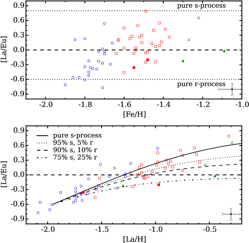
Figure 17.— Top: this panel shows the correlation between [La/Eu] and [Fe/H] for all NGC 6273 stars observed in this work and Johnson et al. (2015a). The colors and symbols are the same as in Figure 12. The dotted lines indicate the pure r–process and pure s–process [La/Eu] abundances from Kappeler et al. (1989) and Bisterzo et al. (2010), respectively. Bottom: similar to Figure 10 in Johnson et al. (2015a) and following McWilliam et al. (2013), this panel plots [La/Eu] as a function of [La/H]. The solid black line indicates the expected change in [La/Eu] as a function of [La/H] when pure s–process material is added to an initial composition of pure r–process material. The dotted, dashed, and dot–dashed dilution curves represent constant mixtures of 95$\%$(s)/5$\%$(r), 90$\%$(s)/10$\%$(r), and 75$\%$(s)/25$\%$(r) material added to an initial r–process composition. Note that the “low–$\alpha$” stars tend to have low [La/Eu] ratios compared to stars with similar [La/H] or [Fe/H].

Interestingly, the low–$\alpha$ stars in Figure 16 either have [La/Fe] $\sim$ 0.6 dex and [Eu/Fe] $\sim$ 0.7 dex or [La/Fe] $\sim$ 0.0 dex and [Eu/Fe] $\sim$ 0.2 dex. Although the origin of these stars is not clear, it is tempting to speculate that two different formation channels may exist (e.g., in situ versus accretion). We note in particular that low–$\alpha$ stars with high [La/Fe] and [Eu/Fe] are found in the Sagittarius field (e.g., McWilliam et al. 2013), albeit at higher [Fe/H]. The existence of these stars further strengthens the idea that at least some of the low–$\alpha$ stars in NGC 6273 could have been accreted from a surrounding field population. The low–$\alpha$ stars with lower [La/Fe] and [Eu/Fe] are perhaps a bigger puzzle, but they could have been formed in situ and preferentially enriched by Type Ia SNe or massive stars with peculiar enrichment signatures. However, Figure 17 shows that all of the low–$\alpha$ stars have about the same [La/Eu] ratios, and may even fall on a separate enrichment sequence. In any case, the simple dilution model shown in Figure 17 suggests that the low–$\alpha$ stars experienced significant r–process enrichment compared to a majority of the $\alpha$–enhanced metal–intermediate and metal–rich cluster stars.

5.4. A Connection Between Blue Hook Stars and Cluster Formation?

NGC 6273 has long been known to exhibit a peculiar HB morphology that includes a very extended blue HB, a clear gap near temperatures of $\sim$20,000 K, and a large population of blue hook stars (Piotto et al. 1999; Brown et al. 2001, 2010; Momany et al. 2004). We confirm these features with new HST color–magnitude diagrams in Figure 14, and find that NGC 6273’s HB includes several distinct groups. Although a detailed examination of each HB group is beyond the scope of this paper, we draw attention to NGC 6273’s large blue hook population in the context of its complex formation history.

Blue hook stars are among the hottest core He burning stars in old globular clusters, and are thought to form when stars reach the RGB–tip with masses low enough to delay the core He flash until after a star reaches the white dwarf cooling sequence (e.g., D’Cruz et al. 1996; Moehler et al. 2000; Brown et al. 2010). The presence of blue hook stars is known to correlate with cluster mass (Rosenberg et al. 2004; Dieball et al. 2009; Brown et al. 2010, 2016), which we illustrate in Figure 18 by showing that both the ratio of blue hook to canonical HB stars ($\frac{N_{BHk}}{N_{HB}}$) and the raw number of blue hook stars (N_BHk) is higher in the more massive clusters. However, He enhancement is also likely tied to blue hook formation (e.g., D’Antona et al. 2002; Tailo et al. 2015).

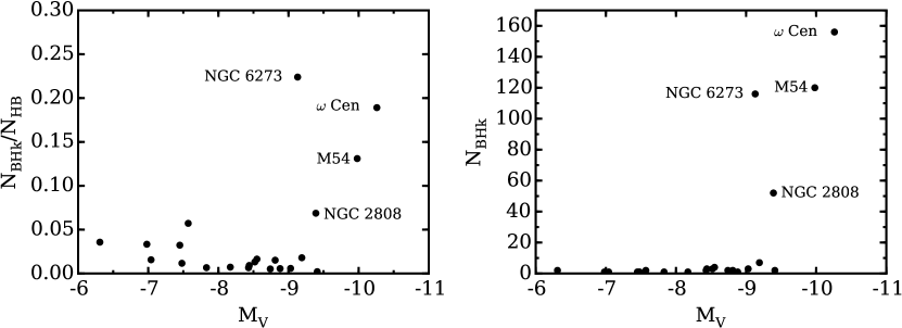
Figure 18.— Left: the ratio of blue hook (BHk) to total HB stars for several Galactic globular clusters is plotted as a function of absolute magnitude (M_V). Except for NGC 6273, the data are taken from Table 1 of Brown et al. (2016). Note that NGC 2419 is not shown, but is known to host a large number of BHk stars as well (e.g., Dieball et al. 2009). Right: the raw number of detected BHk stars is plotted as a function of absolute magnitude for the same cluster sample. Both panels indicate that high masses and large populations of BHk stars distinguish NGC 6273, $\omega$ Cen, M 54, and NGC 2808 from most clusters in the Galaxy.

Although present day cluster mass and the level of He–enrichment strongly correlate with the presence of blue hook stars, neither parameter nor a combination of the two parameters seems adequate to completely predict blue hook formation. For example, He enrichment scenarios (e.g., D’Antona et al. 2010) are presently unable to explain the significant carbon enhancements that are found in He–enhanced blue hook stars (Moehler et al. 2007, 2011; Latour et al. 2014), and Figure 18 shows that clusters with similar absolute magnitudes (proxies for masses) can have vastly different blue hook populations. To illustrate this point, we note that the iron–complex clusters NGC 6273 and M 2 differ by only 0.1 magnitudes in M_V, have similarly extended blue HB morphologies, exhibit comparable light and heavy element abundance variations, have similar average metallicities and ages, and have total HB counts that agree to within 0.5$\%$, but M 2 has a $\frac{N_{BHk}}{N_{HB}}$ ratio of 0.006 (3 blue hook stars) whereas NGC 6273 has $\frac{N_{BHk}}{N_{HB}}$ = 0.224 ($\sim$ 120 blue hook stars). Furthermore, dynamical and binary star evolutionary processes may be ruled out as explanations because the blue hook stars in clusters with large $\frac{N_{BHk}}{N_{HB}}$ ratios, including NGC 6273, do not exhibit radial gradients (e.g., Bedin et al. 2000; Brown et al. 2010). Therefore, additional parameters must play a role in producing blue hook stars.

Interestingly, the three objects in Figure 18 that contain $>$ 100 blue hook stars and have $\frac{N_{BHk}}{N_{HB}}$ $>$ 0.10 are the iron–complex clusters NGC 6273, M 54, and $\omega$ Cen. All three clusters have about the same average metallicity, have large metallicity spreads, and exhibit extreme variations in light element, heavy element, and (most likely) He abundances. However, at least $\omega$ Cen and M 54 are particularly noteworthy because these clusters are strongly suspected to have extragalactic origins (e.g., Bekki & Freeman 2003; Mackey & van den Bergh 2005). The similar chemical pattern and HB morphology that NGC 6273 shares with $\omega$ Cen and M 54 suggest that NGC 6273 may have also been accreted by the Milky Way. If these clusters are all remnants of dwarf galaxy systems, then it is reasonable to assume that each cluster has experienced significant mass loss. Therefore, a cluster’s formation environment and initial mass may play critical roles in forming large populations of blue hook stars, and the different blue hook populations of NGC 6273 and M 2 could be explained if NGC 6273 was initially much more massive than M 2 and/or formed in a different environment. In this context, we note that NGC 2419 and NGC 2808 would also be candidates that may have formed with much larger initial masses, and their higher and lower $\frac{N_{BHk}}{N_{HB}}$ ratios compared to NGC 6273 could be driven by their lower and higher respective metallicities. At least for NGC 2419, there are also some indications that the cluster may have an extragalactic origin (Mackey & van den Bergh 2005).

6. SUMMARY

We have measured detailed abundances, CaT metallicities, and/or radial velocities for $>$ 800 RGB stars ($>$ 300 members) near the massive bulge globular cluster NGC 6273. The abundances and velocities are based on an analysis of high resolution (R $\approx$ 27,000) spectra obtained with the Magellan–M2FS multi–fiber instrument, and includes additional metallicity and velocity measurements of R $\approx$ 18,000 archival VLT–FLAMES CaT spectra. The new data extend the spectroscopic work of Johnson et al. (2015a) and Yong et al. (2016) and span a broad range in luminosity and color. These data are complemented by photometric measurements of new HST–WFC3/UVIS data in the F336W, F438W, F555W, and F814W bands that extend from the RGB–tip down to at least 2 magnitudes below the main–sequence turn–off.

A simple kinematic analysis indicates that $\sim$40$\%$ of our spectroscopic targets are cluster members and have heliocentric radial velocities between $+$120 and $+$170 km s^-1. We find a cluster average velocity of $+$144.71 km s^-1 and a dispersion of 8.57 km s^-1. The cluster exhibits net rotation with a mean projected amplitude of 3.83 km s^-1. A Plummer model fit to the projected radial velocity dispersion profile suggests that NGC 6273 has a central velocity dispersion of at least 10–12 km s^-1 and an A_rot./$\sigma$_o ratio of $\sim$0.30–0.35.

The [Fe/H] abundances presented here follow the results of Johnson et al. (2015a), Han et al. (2015), and Yong et al. (2016) that suggest an intrinsic metallicity spread exists in NGC 6273. Using EW measurements of individual Fe I and Fe II lines, we find evidence that at least three stellar populations with different [Fe/H] may exist: (1) a metal–poor group with [Fe/H] $\leq$ –1.65; (2) a metal–intermediate group with –1.65 $<$ [Fe/H] $\leq$ –1.35; and (3) a metal–rich group with [Fe/H] $>$ –1.35. The metal–poor and metal–intermediate populations may be associated with different giant branches, and both populations may contain roughly equivalent numbers of stars. In contrast, the metal–rich population only constitutes 6$\%$ of our sample. The metal–intermediate stars may also be more centrally concentrated than the metal–poor stars, but the radial distribution differences are only observed at projected distances $\gtrsim$1.5$\arcmin$ from the cluster center. Similar to Yong et al. (2016), our CaT measurements extend the metal–rich tail to at least [Fe/H] = –1.0 to –0.5 dex, but it is possible that some (or all) of these comparatively very metal–rich stars could be bulge field stars with velocities in the membership range.

The cluster’s chemical abundance patterns indicate that all three major populations contain distinct sets of first (Na/Al–poor) and second (Na/Al–rich) generation stars. All three populations exhibit similar Na–Al correlations, but the [Mg/Fe] and [Al/Fe] distributions suggest a complex enrichment scenario. For example, [Al/Fe] spans about a factor of 10 in abundance for the metal–poor and metal–intermediate populations, but only the metal–intermediate stars show evidence of a Mg–Al anti–correlation. The metal–rich stars may also exhibit a Mg–Al anti–correlation, but the sample size is too small to draw any strong conclusions. In confirmed, a change in the Mg–Al distribution as a function of metallicity may suggest that the gas from which the metal–intermediate and metal–rich second generation stars formed was processed at higher temperatures than the gas from which the metal–poor second generation stars formed. Notably, we did not observe any significant correlations between Mg/Al and Si that would have indicated burning temperatures significantly higher than $\sim$65–70 MK, as is the case in several other massive clusters. Interestingly, the metal–intermediate and metal–rich stars with [Al/Fe] $>$ 1.0 dex have higher than expected [Mg/Fe] abundances, which could indicate that the gas from which these stars formed was polluted by a different class or mass range of objects.

Further examination of the light element abundances indicates that the RGB and AGB stars may not have identical [Na/Fe] and [Al/Fe] distributions. In particular, we did not find any AGB stars with [Na/Fe] $>$ 0.5 dex or [Al/Fe] $>$ 1.0 dex. The “missing” AGB stars account for $\sim$30$\%$ of the RGB sample, which is close to the fraction of extreme HB and blue hook stars relative to the total HB population. We speculate that the RGB stars with the highest [Na/Fe] and [Al/Fe] abundances likely evolve to become extreme HB or blue hook stars and do not ascend the AGB.

The overall [$\alpha$/Fe] ratios may slowly decline with increasing metallicity, but most stars have [$\alpha$/Fe] $\sim$ 0.3 dex. Additionally, the Fe–peak elements exhibit solar [X/Fe] ratios, regardless of metallicity, and the star–to–star dispersion is $\sim$0.1 dex in all three populations. In contrast, the heavy s–process element La exhibits a correlated increase with metallicity that ranges from [La/Fe] $\sim$ –0.2 dex at the lowest metallicities to [La/Fe] $\sim$ 0.8 dex at the highest metallicities. However, the r–process element Eu maintains a constant abundance of [Eu/Fe] $\sim$ 0.4 dex across the full [Fe/H] range. In agreement with Johnson et al. (2015a), we find that the correlated increase in [La/Eu] with metallicity is consistent with a nearly pure s–process enrichment pattern. Constant r–process production is required to maintain the flat [Eu/Fe] abundance distribution, but the r–process contribution likely does not significantly exceed $\sim$10$\%$. Therefore, we confirm that NGC 6273 shares an almost identical s–process enrichment pattern with other iron–complex clusters such as $\omega$ Cen, M 2, M 22, and NGC 5286.

We have also identified a population of at least 5 peculiar “low–$\alpha$” stars that have [$\alpha$/Fe] $\sim$ 0.0 dex, low [Na/Fe] and [Al/Fe] abundances (all are first generation stars), and low [La/Eu] ratios. Many, but not all, of the low–$\alpha$ stars also exhibit low [Cr/Fe] and [Ni/Fe] abundances. Although the metal–poor population does not contain any low–$\alpha$ stars, the specific frequency of low–$\alpha$ stars increases from 9$\%$ in the metal–intermediate population to 50$\%$ in the metal–rich population. However, the ratios of low–$\alpha$ stars in each population should be confirmed with future large sample observations. Interestingly, the combination of $\alpha$–enhanced and $\alpha$–poor stars in NGC 6273 closely resembles the M 54 and Sagittarius field star system, and we speculate that some or all of the low–$\alpha$ stars may have been accreted from a former field population that surrounded the NGC 6273 core but had different chemistry. We note that similar populations may also be present in at least $\omega$ Cen, M 2, and NGC 5286.

An examination of NGC 6273’s HB revealed a particularly complex morphology. We find that the HB is composed of several distinct groups of stars with different masses, and that the mass range within each of the extreme HB and blue hook populations varies by $\lesssim$ 0.01 M_⊙. Interestingly, the HST data show that NGC 6273 may have one of the largest blue hook populations in the Galaxy. In particular, the ratio of blue hook to canonical HB stars is $\sim$0.22, which is a trait shared only by $\omega$ Cen, M 54, NGC 2419, and NGC 2808. Since all of these clusters are very massive, and at least $\omega$ Cen, M 54, and NGC 2419 are suspected to have extragalactic origins, we speculate that a cluster’s initial mass and formation environment are likely critical factors in the production of blue hook stars, at least in large numbers.

Table 1Observing Log

Field	Telescope/Instrument	Setup	UT Date	Exposure
				(s)
Spectroscopy
1a	VLT$-$FLAMES	HR21	2014 April 13	1 $\times$ 2445
1b	VLT$-$FLAMES	HR21	2014 May 7	1 $\times$ 2445
2a	VLT$-$FLAMES	HR21	2014 July 13	1 $\times$ 2445
2b	VLT$-$FLAMES	HR21	2014 August 2	1 $\times$ 2445
3a	VLT$-$FLAMES	HR21	2014 July 21	1 $\times$ 2445
3b	VLT$-$FLAMES	HR21	2014 August 13	1 $\times$ 2445
4	Magellan$-$M2FS	CaT	2015 July 17	4 $\times$ 1200
5	Magellan$-$M2FS	CaT	2015 July 20	3 $\times$ 1800
6	Magellan$-$M2FS	Bulge$\_$GC1	2015 July 21	6 $\times$ 1800
7	Magellan$-$M2FS	Bulge$\_$GC1	2015 July 22	6 $\times$ 1800
Photometry
1	HST$-$WFC3/UVIS	F336W	2016 March 13	4 $\times$ 350
$\cdots$	HST$-$WFC3/UVIS	F336W	2016 March 13	1 $\times$ 566, 659, 674, 685
$\cdots$	HST$-$WFC3/UVIS	F438W	2016 March 13	2 $\times$ 10
$\cdots$	HST$-$WFC3/UVIS	F438W	2016 March 13	4 $\times$ 350
$\cdots$	HST$-$WFC3/UVIS	F555W	2016 March 13	4 $\times$ 10
$\cdots$	HST$-$WFC3/UVIS	F555W	2016 March 13	4 $\times$ 350
$\cdots$	HST$-$WFC3/UVIS	F814W	2016 March 13	2 $\times$ 10
$\cdots$	HST$-$WFC3/UVIS	F814W	2016 March 13	4 $\times$ 350

Table 2Star Identifiers, Coordinates, Photometry, and Radial Velocities for NGC 6273 Members

Star Name	RA	DEC	J	KS	RVhelio.	RV Error
(2MASS)	(degrees)	(degrees)	(mag.)	(mag.)	(km s-1)	(km s-1)
Bulge$\_$GC1 Members
17022227$-$2613433	255.592801	$-$26.228718	10.882	9.920	142.87	0.16
17022817$-$2616426	255.617398	$-$26.278500	11.893	11.102	156.50	0.23
17022912$-$2617443	255.621349	$-$26.295652	11.153	10.218	143.61	0.18
17023087$-$2618515	255.628646	$-$26.314312	11.891	11.103	149.94	0.27
17023192$-$2614177	255.633037	$-$26.238272	10.451	9.434	125.82	0.21
17023225$-$2614521	255.634399	$-$26.247812	11.764	10.896	123.72	0.19
17023338$-$2617104	255.639093	$-$26.286234	12.075	11.262	143.75	0.37
17023342$-$2616165	255.639279	$-$26.271273	11.484	10.628	125.67	0.27
17023346$-$2616375	255.639422	$-$26.277109	12.050	11.225	158.46	0.25
17023388$-$2607556	255.641177	$-$26.132128	12.063	11.254	142.01	0.21
17023394$-$2616196	255.641453	$-$26.272135	10.444	9.470	140.13	0.24
17023435$-$2616386	255.643127	$-$26.277416	10.450	9.492	139.07	0.16
17023459$-$2615560	255.644129	$-$26.265577	11.003	10.038	145.69	0.18
17023460$-$2616038	255.644175	$-$26.267748	11.581	10.699	158.87	0.23
17023517$-$2616130	255.646543	$-$26.270304	11.198	10.275	158.23	0.20
17023523$-$2617058	255.646802	$-$26.284969	11.228	10.286	145.64	0.21
17023529$-$2613089	255.647075	$-$26.219151	11.479	10.644	146.24	0.18
17023551$-$2616175	255.647962	$-$26.271542	11.843	10.955	146.99	0.42
17023583$-$2616444	255.649297	$-$26.279018	12.021	11.207	160.90	0.26
17023589$-$2615218	255.649556	$-$26.256058	12.151	11.162	147.53	0.25
17023595$-$2615342	255.649809	$-$26.259501	10.513	9.418	135.85	0.34
17023618$-$2616576	255.650765	$-$26.282686	11.889	11.035	143.86	0.24
17023685$-$2616454	255.653554	$-$26.279297	11.996	11.213	127.85	0.24
17023694$-$2615130	255.653936	$-$26.253637	11.818	11.030	136.24	0.28
17023720$-$2614581	255.655012	$-$26.249496	12.071	11.277	148.74	0.26
17023723$-$2617063	255.655138	$-$26.285105	10.929	10.020	153.73	0.15
17023728$-$2617024	255.655371	$-$26.284014	11.666	10.795	126.49	0.24
17023744$-$2615306	255.656031	$-$26.258522	11.703	10.886	157.83	0.31
17023783$-$2615095	255.657643	$-$26.252665	11.869	10.960	136.62	0.52
17023898$-$2618010	255.662443	$-$26.300289	11.941	11.122	128.05	0.25
17023916$-$2616500	255.663203	$-$26.280567	10.917	9.957	141.22	0.22
17023938$-$2619361	255.664089	$-$26.326698	11.913	11.098	148.66	0.26
17023943$-$2615343	255.664313	$-$26.259535	10.995	10.094	127.67	0.23
17023946$-$2615017	255.664417	$-$26.250486	11.848	10.998	137.08	0.29
17023956$-$2617202	255.664850	$-$26.288948	12.018	11.083	142.02	0.27
17023984$-$2617360	255.666020	$-$26.293348	11.535	10.647	156.17	0.27
17023993$-$2616370	255.666382	$-$26.276957	10.896	9.953	165.14	0.45
17024016$-$2615588	255.667372	$-$26.266354	11.462	10.566	136.51	0.56
17024032$-$2617400	255.668040	$-$26.294472	11.451	10.618	133.88	0.22
17024041$-$2617149	255.668397	$-$26.287489	11.241	10.052	143.46	0.25
17024104$-$2616507	255.671004	$-$26.280752	11.803	10.990	142.50	0.25
17024128$-$2616015	255.672018	$-$26.267092	11.963	11.068	155.21	1.03
17024132$-$2613517	255.672190	$-$26.231030	11.706	10.876	137.65	0.29
17024153$-$2621081	255.673077	$-$26.352268	10.462	9.473	147.53	0.22
17024165$-$2617033	255.673565	$-$26.284258	11.239	10.359	148.00	0.31
17024173$-$2616245	255.673916	$-$26.273491	10.895	9.846	133.46	0.19
17024226$-$2615137	255.676124	$-$26.253811	12.179	11.297	152.85	0.30
17024242$-$2615557	255.676779	$-$26.265476	10.955	9.960	147.05	0.16
17024289$-$2615274	255.678722	$-$26.257622	11.501	10.652	135.21	0.30
17024371$-$2620183	255.682141	$-$26.338444	11.811	10.980	148.99	0.35
17024377$-$2615526	255.682380	$-$26.264633	11.366	10.361	144.50	0.28
17024412$-$2616495	255.683863	$-$26.280443	11.736	10.802	139.54	0.19
17024416$-$2615177	255.684021	$-$26.254919	11.384	10.502	136.71	0.29
17024472$-$2615190	255.686341	$-$26.255291	12.247	11.286	143.96	0.28
17024566$-$2615124	255.690259	$-$26.253452	11.160	10.221	139.12	0.26
17024625$-$2610100	255.692748	$-$26.169458	11.834	11.051	138.95	0.21
17024627$-$2614484	255.692832	$-$26.246792	10.832	9.900	142.65	0.38
17024838$-$2615546	255.701584	$-$26.265182	10.519	9.441	140.39	0.37
17025033$-$2615582	255.709727	$-$26.266191	11.667	10.714	142.70	0.24
M2FS Calcium Triplet Members
17015056$-$2616256	255.460689	$-$26.273787	13.115	12.200	158.39	0.79
17021380$-$2613223	255.557535	$-$26.222864	12.771	12.166	144.01	1.03
17021778$-$2616058	255.574110	$-$26.268282	12.586	11.894	147.14	1.55
17022040$-$2616289	255.585022	$-$26.274719	11.532	10.744	151.61	0.57
17022227$-$2613433	255.592801	$-$26.228718	10.882	9.920	143.37	0.41
17022395$-$2614538	255.599796	$-$26.248289	11.721	10.898	148.00	0.55
17022413$-$2619124	255.600561	$-$26.320137	12.688	11.994	154.67	1.01
17022442$-$2616495	255.601752	$-$26.280430	10.439	9.516	143.67	0.48
17022511$-$2617141	255.604652	$-$26.287275	12.857	12.099	154.45	1.70
17022611$-$2614059	255.608832	$-$26.234976	12.182	11.347	144.28	0.52
17022652$-$2616283	255.610513	$-$26.274536	13.010	12.288	159.21	1.50
17022653$-$2616064	255.610553	$-$26.268448	11.198	10.422	140.49	0.62
17022656$-$2615506	255.610675	$-$26.264078	13.196	12.293	142.32	5.00
17022685$-$2615055	255.611910	$-$26.251530	12.699	11.872	149.65	1.55
17022743$-$2611593	255.614321	$-$26.199825	12.759	12.054	142.53	1.09
17022766$-$2617054	255.615261	$-$26.284859	12.163	11.372	147.18	0.62
17022785$-$2615555	255.616065	$-$26.265430	11.692	10.792	144.98	0.89
17022817$-$2616426	255.617398	$-$26.278500	11.893	11.102	159.24	0.73
17022822$-$2615181	255.617601	$-$26.255043	12.709	11.934	149.11	2.08
17022862$-$2615368	255.619277	$-$26.260242	12.802	11.982	140.06	0.80
17022878$-$2614320	255.619947	$-$26.242231	11.304	10.393	146.63	0.51
17022899$-$2614057	255.620825	$-$26.234924	12.846	12.130	149.05	2.14
17022912$-$2617443	255.621349	$-$26.295652	11.153	10.218	145.24	0.56
17022918$-$2616135	255.621616	$-$26.270433	13.080	12.293	155.43	0.83
17022948$-$2616533	255.622852	$-$26.281483	12.638	11.906	136.96	0.66
17023046$-$2616292	255.626919	$-$26.274801	12.375	11.591	147.27	0.68
17023059$-$2617449	255.627478	$-$26.295811	12.787	12.106	154.20	0.95
17023059$-$2613524	255.627493	$-$26.231232	13.001	12.226	136.00	1.12
17023078$-$2615183	255.628290	$-$26.255096	11.631	10.737	158.75	1.08
17023087$-$2618515	255.628646	$-$26.314312	11.891	11.103	152.23	0.64
17023090$-$2616159	255.628753	$-$26.271109	12.512	11.736	136.34	0.91
17023104$-$2615040	255.629374	$-$26.251123	12.446	11.628	124.56	2.40
17023155$-$2616336	255.631499	$-$26.276005	12.744	11.971	147.07	0.64
17023158$-$2617259	255.631607	$-$26.290541	11.412	10.550	159.34	0.44
17023188$-$2613529	255.632858	$-$26.231380	12.679	11.902	143.87	1.09
17023192$-$2614177	255.633037	$-$26.238272	10.451	9.434	128.45	0.80
17023203$-$2617557	255.633462	$-$26.298817	12.830	12.113	138.00	0.71
17023225$-$2614521	255.634399	$-$26.247812	11.764	10.896	124.86	0.60
17023227$-$2608256	255.634478	$-$26.140467	12.530	11.847	139.35	2.62
17023254$-$2615142	255.635623	$-$26.253952	12.630	11.886	154.99	1.57
17023282$-$2614423	255.636763	$-$26.245098	12.769	12.006	152.55	1.22
17023286$-$2616339	255.636945	$-$26.276089	12.568	11.781	154.58	0.68
17023286$-$2616475	255.636949	$-$26.279886	11.258	10.410	133.39	0.77
17023289$-$2615535	255.637042	$-$26.264864	11.103	10.181	159.02	0.87
17023293$-$2616127	255.637211	$-$26.270214	11.801	10.988	143.15	1.14
17023295$-$2619582	255.637305	$-$26.332838	12.792	12.074	156.12	1.13
17023301$-$2615360	255.637556	$-$26.260017	11.211	10.264	141.91	1.22
17023337$-$2617312	255.639045	$-$26.292023	12.302	11.592	157.05	0.74
17023338$-$2617104	255.639093	$-$26.286234	12.075	11.262	146.05	0.53
17023365$-$2613419	255.640223	$-$26.228317	12.101	11.344	144.79	0.91
17023384$-$2616416	255.641002	$-$26.278240	11.785	10.952	143.13	1.12
17023385$-$2616533	255.641050	$-$26.281485	12.463	11.684	130.99	1.14
17023388$-$2607556	255.641177	$-$26.132128	12.063	11.254	143.60	0.82
17023402$-$2614410	255.641780	$-$26.244724	12.851	12.070	145.30	1.47
17023403$-$2616245	255.641831	$-$26.273497	12.904	12.244	146.19	1.80
17023424$-$2615437	255.642703	$-$26.262144	10.977	10.000	154.03	0.42
17023443$-$2614277	255.643479	$-$26.241035	12.187	11.339	144.51	0.93
17023447$-$2616155	255.643650	$-$26.270983	12.214	11.324	160.44	0.79
17023448$-$2614097	255.643669	$-$26.236055	12.233	11.611	141.06	2.38
17023454$-$2616292	255.643934	$-$26.274790	10.760	9.771	141.81	0.39
17023455$-$2614515	255.643993	$-$26.247656	12.321	11.563	146.70	1.75
17023456$-$2612318	255.644008	$-$26.208836	12.647	11.928	146.27	1.37
17023459$-$2614235	255.644126	$-$26.239876	12.539	11.724	158.56	2.09
17023459$-$2615560	255.644129	$-$26.265577	11.003	10.038	146.30	0.49
17023471$-$2617228	255.644647	$-$26.289673	12.511	11.723	156.79	0.64
17023472$-$2616381	255.644670	$-$26.277250	12.956	12.105	148.51	1.76
17023481$-$2617152	255.645044	$-$26.287563	11.415	10.535	148.21	1.03
17023502$-$2616017	255.645941	$-$26.267157	12.710	12.075	128.49	2.21
17023506$-$2615148	255.646085	$-$26.254122	12.770	11.964	131.51	1.53
17023509$-$2616406	255.646228	$-$26.277952	11.098	10.182	145.66	0.51
17023516$-$2619262	255.646540	$-$26.323950	12.414	11.644	146.81	0.63
17023518$-$2613595	255.646621	$-$26.233206	13.091	12.287	150.73	1.52
17023529$-$2613089	255.647075	$-$26.219151	11.479	10.644	148.75	0.50
17023544$-$2613120	255.647679	$-$26.220001	12.318	11.615	137.42	1.51
17023548$-$2616113	255.647873	$-$26.269812	11.906	10.946	162.46	1.31
17023558$-$2615298	255.648291	$-$26.258282	12.487	11.689	141.03	2.60
17023564$-$2617078	255.648536	$-$26.285519	12.644	11.914	136.31	0.63
17023568$-$2614537	255.648673	$-$26.248266	12.829	12.146	144.07	1.31
17023572$-$2614154	255.648862	$-$26.237619	12.924	12.181	152.51	1.68
17023589$-$2615218	255.649556	$-$26.256058	12.151	11.162	148.39	1.47
17023589$-$2610118	255.649574	$-$26.169950	12.554	11.780	146.50	1.22
17023595$-$2615342	255.649809	$-$26.259501	10.513	9.418	134.97	1.30
17023595$-$2616260	255.649826	$-$26.273914	12.495	11.723	149.15	1.08
17023618$-$2616576	255.650765	$-$26.282686	11.889	11.035	129.80	0.53
17023647$-$2614434	255.651984	$-$26.245413	12.466	11.744	151.46	2.43
17023658$-$2617338	255.652419	$-$26.292744	12.363	11.538	153.78	0.67
17023670$-$2613247	255.652938	$-$26.223528	12.750	12.009	120.29	1.80
17023670$-$2615336	255.652952	$-$26.259346	12.982	11.971	153.79	1.88
17023678$-$2615189	255.653270	$-$26.255266	12.652	11.822	136.01	1.92
17023685$-$2616454	255.653554	$-$26.279297	11.996	11.213	145.07	0.43
17023686$-$2616559	255.653599	$-$26.282219	13.042	12.068	153.61	0.97
17023689$-$2614208	255.653720	$-$26.239138	12.760	11.998	144.47	2.15
17023694$-$2615130	255.653936	$-$26.253637	11.818	11.030	137.88	0.96
17023715$-$2614342	255.654797	$-$26.242859	12.907	12.174	144.78	2.58
17023720$-$2614581	255.655012	$-$26.249496	12.071	11.277	149.65	1.36
17023723$-$2617063	255.655138	$-$26.285105	10.929	10.020	154.70	0.70
17023744$-$2615306	255.656031	$-$26.258522	11.703	10.886	159.69	0.94
17023765$-$2618162	255.656899	$-$26.304520	12.123	11.377	153.06	0.66
17023781$-$2616375	255.657547	$-$26.277088	10.541	9.651	141.94	0.54
17023783$-$2615095	255.657643	$-$26.252665	11.869	10.960	139.24	5.51
17023783$-$2614577	255.657657	$-$26.249386	12.682	11.833	143.52	1.60
17023799$-$2615204	255.658324	$-$26.255690	12.690	12.013	146.26	1.53
17023810$-$2618176	255.658780	$-$26.304892	12.839	12.180	154.70	0.75
17023811$-$2617392	255.658832	$-$26.294239	11.678	10.890	137.44	0.86
17023856$-$2617209	255.660695	$-$26.289145	10.980	10.134	143.98	1.09
17023868$-$2616516	255.661183	$-$26.281012	11.323	10.400	138.09	1.11
17023874$-$2612434	255.661456	$-$26.212059	11.396	10.542	145.28	0.75
17023883$-$2617141	255.661802	$-$26.287258	12.996	12.172	144.08	0.81
17023898$-$2615168	255.662422	$-$26.254679	12.692	12.049	140.17	2.83
17023898$-$2618010	255.662443	$-$26.300289	11.941	11.122	129.60	0.86
17023907$-$2614332	255.662799	$-$26.242571	12.683	11.981	137.89	2.15
17023916$-$2619223	255.663204	$-$26.322882	12.836	12.104	152.74	0.72
17023935$-$2617492	255.663974	$-$26.297014	12.765	12.004	144.24	0.98
17023946$-$2615017	255.664417	$-$26.250486	11.848	10.998	137.86	0.96
17023949$-$2614427	255.664579	$-$26.245205	12.270	11.263	143.95	1.37
17023955$-$2614223	255.664816	$-$26.239548	12.695	11.995	127.70	1.88
17023956$-$2617202	255.664850	$-$26.288948	12.018	11.083	144.06	0.69
17023968$-$2618186	255.665352	$-$26.305193	12.859	12.153	133.95	0.87
17023984$-$2617360	255.666020	$-$26.293348	11.535	10.647	156.30	0.73
17023990$-$2614560	255.666270	$-$26.248898	12.964	12.175	142.62	2.32
17023991$-$2615483	255.666307	$-$26.263420	12.469	11.777	149.34	1.41
17023993$-$2616370	255.666382	$-$26.276957	10.896	9.953	163.24	0.91
17023993$-$2617269	255.666411	$-$26.290812	12.358	11.707	157.78	0.69
17024014$-$2613327	255.667265	$-$26.225773	10.621	9.737	148.25	0.47
17024016$-$2616096	255.667344	$-$26.269346	11.416	10.451	126.81	0.53
17024023$-$2613150	255.667652	$-$26.220848	12.638	11.922	142.33	1.25
17024041$-$2617149	255.668397	$-$26.287489	11.241	10.052	143.85	0.92
17024045$-$2616145	255.668555	$-$26.270721	12.433	11.690	147.88	1.04
17024054$-$2616363	255.668932	$-$26.276772	12.664	11.781	141.11	0.65
17024062$-$2615215	255.669285	$-$26.255985	12.979	12.128	147.54	1.07
17024082$-$2617217	255.670123	$-$26.289385	12.674	11.916	143.00	0.73
17024107$-$2614455	255.671132	$-$26.245989	12.253	11.436	122.53	1.37
17024114$-$2616396	255.671447	$-$26.277679	11.466	10.521	149.24	0.44
17024116$-$2613328	255.671538	$-$26.225796	12.744	12.049	146.74	1.69
17024119$-$2614325	255.671644	$-$26.242380	12.450	11.687	137.55	1.63
17024128$-$2616015	255.672018	$-$26.267092	11.963	11.068	148.19	0.47
17024132$-$2613517	255.672190	$-$26.231030	11.706	10.876	137.67	0.64
17024139$-$2616441	255.672491	$-$26.278927	12.971	12.295	144.23	0.94
17024148$-$2614569	255.672851	$-$26.249151	12.467	11.676	137.96	2.01
17024149$-$2615400	255.672905	$-$26.261124	12.295	11.500	138.61	1.01
17024153$-$2621081	255.673077	$-$26.352268	10.462	9.473	147.55	0.79
17024156$-$2616535	255.673172	$-$26.281544	12.042	11.193	138.23	1.02
17024173$-$2616245	255.673916	$-$26.273491	10.895	9.846	134.37	0.40
17024177$-$2619095	255.674057	$-$26.319324	12.900	12.095	151.29	0.68
17024182$-$2616157	255.674276	$-$26.271055	12.953	12.174	147.55	1.32
17024203$-$2616300	255.675134	$-$26.275007	12.713	11.890	126.37	0.76
17024205$-$2616025	255.675249	$-$26.267378	12.467	11.575	136.57	0.70
17024272$-$2615570	255.678003	$-$26.265837	12.281	11.427	145.59	0.91
17024272$-$2616411	255.678020	$-$26.278093	12.180	11.216	160.88	0.60
17024289$-$2615274	255.678722	$-$26.257622	11.501	10.652	138.15	0.76
17024298$-$2616421	255.679095	$-$26.278376	13.083	12.135	143.38	0.71
17024325$-$2618436	255.680249	$-$26.312134	12.429	11.619	128.06	0.71
17024326$-$2617504	255.680281	$-$26.297361	11.864	10.982	124.88	1.15
17024371$-$2620183	255.682141	$-$26.338444	11.811	10.980	149.07	1.09
17024377$-$2615526	255.682380	$-$26.264633	11.366	10.361	146.20	0.95
17024403$-$2616575	255.683469	$-$26.282656	12.303	11.506	139.89	0.70
17024412$-$2616495	255.683863	$-$26.280443	11.736	10.802	139.26	0.57
17024427$-$2615464	255.684480	$-$26.262892	13.053	12.248	133.83	1.19
17024453$-$2618589	255.685572	$-$26.316368	12.827	11.978	155.13	0.62
17024453$-$2616377	255.685573	$-$26.277155	11.288	10.307	142.93	0.37
17024468$-$2614354	255.686186	$-$26.243177	12.206	11.433	142.67	0.80
17024472$-$2615190	255.686341	$-$26.255291	12.247	11.286	145.33	0.82
17024510$-$2617163	255.687955	$-$26.287874	12.652	11.828	150.74	0.84
17024533$-$2616536	255.688884	$-$26.281574	12.883	12.097	149.04	0.72
17024538$-$2613360	255.689091	$-$26.226677	12.174	11.344	146.43	0.75
17024566$-$2615124	255.690259	$-$26.253452	11.160	10.221	138.19	0.70
17024575$-$2616148	255.690665	$-$26.270800	12.464	11.597	127.61	0.87
17024618$-$2615261	255.692427	$-$26.257250	11.284	10.322	161.80	0.74
17024625$-$2610100	255.692748	$-$26.169458	11.834	11.051	140.97	1.54
17024627$-$2614484	255.692832	$-$26.246792	10.832	9.900	142.82	0.72
17024700$-$2603270	255.695862	$-$26.057510	12.596	11.792	159.72	0.67
17024705$-$2616254	255.696052	$-$26.273733	12.515	11.622	141.87	0.87
17024711$-$2617365	255.696295	$-$26.293499	12.983	12.135	148.29	0.72
17024717$-$2615107	255.696559	$-$26.252991	11.566	10.676	153.60	0.97
17024759$-$2615347	255.698309	$-$26.259642	12.507	11.646	139.87	1.67
17024838$-$2615546	255.701584	$-$26.265182	10.519	9.441	140.71	1.09
17024915$-$2617017	255.704820	$-$26.283813	12.734	11.828	143.96	0.61
17024937$-$2616484	255.705737	$-$26.280121	11.208	10.171	144.15	1.67
17024979$-$2613193	255.707474	$-$26.222040	12.971	12.195	140.81	0.83
17025033$-$2615582	255.709727	$-$26.266191	11.667	10.714	143.84	0.86
17025055$-$2616417	255.710665	$-$26.278254	12.934	12.170	155.50	1.07
17025121$-$2617230	255.713406	$-$26.289745	11.079	10.104	135.16	1.47
17025221$-$2614307	255.717545	$-$26.241865	11.807	10.972	148.20	0.49
17025747$-$2616225	255.739472	$-$26.272921	12.978	12.251	157.24	1.08
17025805$-$2621321	255.741895	$-$26.358932	12.219	11.413	147.03	2.39
17025927$-$2616423	255.746968	$-$26.278431	12.817	12.021	141.54	1.16
17030131$-$2623385	255.755462	$-$26.394039	12.575	11.841	150.70	0.73
17030625$-$2603576	255.776051	$-$26.066021	12.699	12.012	131.00	0.97
17030750$-$2618050	255.781290	$-$26.301416	12.831	11.975	149.18	0.82
17030978$-$2608035	255.790766	$-$26.134314	10.499	9.373	120.39	0.50
17032450$-$2614557	255.852104	$-$26.248827	10.792	9.512	151.56	0.94
FLAMES Calcium Triplet Members
17022072$-$2613068	255.586348	$-$26.218561	15.870	15.356	146.49	0.85
17022290$-$2615030	255.595451	$-$26.250839	15.485	14.906	146.86	0.88
17022299$-$2616208	255.595804	$-$26.272467	16.025	15.444	155.37	0.79
17022356$-$2620214	255.598180	$-$26.339283	16.025	15.888	146.34	0.82
17022468$-$2614174	255.602869	$-$26.238173	16.051	15.258	156.49	0.63
17022476$-$2613395	255.603199	$-$26.227661	15.048	14.450	152.88	0.93
17022496$-$2613038	255.604030	$-$26.217739	15.250	14.627	153.10	0.88
17022511$-$2613452	255.604664	$-$26.229237	15.571	15.288	152.28	0.88
17022616$-$2614422	255.609004	$-$26.245073	14.875	14.212	138.40	0.91
17022618$-$2618223	255.609095	$-$26.306217	15.344	14.591	152.83	0.87
17022631$-$2615278	255.609640	$-$26.257738	15.649	15.115	137.70	0.77
17022814$-$2616200	255.617280	$-$26.272230	15.058	14.242	144.32	0.81
17022954$-$2618278	255.623111	$-$26.307735	15.176	14.468	154.66	0.87
17023007$-$2615408	255.625333	$-$26.261353	15.527	14.884	145.73	0.91
17023077$-$2616496	255.628223	$-$26.280451	13.563	12.845	155.97	0.88
17023103$-$2612162	255.629320	$-$26.204500	15.595	14.889	140.82	0.71
17023159$-$2612342	255.631642	$-$26.209511	15.534	15.099	141.42	0.76
17023203$-$2619026	255.633469	$-$26.317402	15.525	14.846	140.81	0.88
17023213$-$2619593	255.633908	$-$26.333143	15.224	14.581	149.16	0.88
17023242$-$2613157	255.635114	$-$26.221052	13.595	12.842	152.39	0.90
17023247$-$2617087	255.635311	$-$26.285761	16.011	15.224	158.55	0.88
17023334$-$2615265	255.638926	$-$26.257368	14.806	14.123	153.41	0.90
17023356$-$2614520	255.639862	$-$26.247795	16.021	14.835	133.89	0.88
17023402$-$2621297	255.641751	$-$26.358276	16.008	13.633	146.46	0.88
17023443$-$2614277	255.643479	$-$26.241035	12.187	11.339	143.41	0.93
17023554$-$2613408	255.648085	$-$26.228025	14.482	13.830	140.54	0.92
17023558$-$2615076	255.648269	$-$26.252123	13.167	12.439	145.52	0.91
17023595$-$2616260	255.649826	$-$26.273914	12.495	11.723	147.64	0.90
17023596$-$2615284	255.649849	$-$26.257910	13.895	13.130	137.80	0.92
17023597$-$2610360	255.649897	$-$26.176682	15.301	14.804	149.50	0.90
17023617$-$2615033	255.650716	$-$26.250921	14.800	14.464	135.85	0.91
17023617$-$2618590	255.650745	$-$26.316404	13.739	13.077	145.31	0.93
17023689$-$2614407	255.653712	$-$26.244640	13.556	12.731	140.04	0.91
17023720$-$2614581	255.655012	$-$26.249496	12.071	11.277	137.44	0.91
17023722$-$2613508	255.655119	$-$26.230783	14.744	14.134	151.69	0.90
17023741$-$2610082	255.655897	$-$26.168961	15.692	14.756	145.75	0.89
17023772$-$2613141	255.657169	$-$26.220608	15.745	14.689	135.68	0.89
17023814$-$2614538	255.658921	$-$26.248301	14.149	13.497	149.23	0.92
17023840$-$2615171	255.660040	$-$26.254765	13.506	13.470	159.52	0.89
17023854$-$2614384	255.660597	$-$26.244015	14.817	14.546	139.36	0.90
17023860$-$2621071	255.660842	$-$26.351995	15.875	14.174	149.15	0.86
17023885$-$2616121	255.661880	$-$26.270037	12.768	11.869	153.65	0.91
17023887$-$2614410	255.661975	$-$26.244740	14.094	13.246	135.41	0.92
17023921$-$2618458	255.663379	$-$26.312729	14.554	13.957	141.96	0.91
17023960$-$2620224	255.665035	$-$26.339567	13.651	12.861	142.37	0.92
17023962$-$2621147	255.665104	$-$26.354101	15.643	14.852	149.40	0.86
17023963$-$2616118	255.665157	$-$26.269972	10.642	9.691	136.94	0.92
17024038$-$2614182	255.668263	$-$26.238403	15.651	15.066	137.71	0.89
17024079$-$2616001	255.669999	$-$26.266697	14.019	13.778	141.58	0.89
17024167$-$2609335	255.673666	$-$26.159330	15.825	14.925	146.03	0.77
17024173$-$2618413	255.673906	$-$26.311478	15.347	14.546	147.48	0.78
17024175$-$2615474	255.673986	$-$26.263186	13.382	12.455	144.06	0.92
17024214$-$2616091	255.675608	$-$26.269211	15.857	15.299	144.18	0.87
17024215$-$2614395	255.675629	$-$26.244328	14.795	14.147	135.03	0.90
17024240$-$2620190	255.676705	$-$26.338614	15.388	14.691	150.96	0.90
17024297$-$2612310	255.679072	$-$26.208635	15.818	15.128	140.72	0.91
17024312$-$2617355	255.679705	$-$26.293217	13.181	12.448	150.36	0.89
17024374$-$2617194	255.682286	$-$26.288733	13.668	12.898	142.68	0.91
17024376$-$2615017	255.682337	$-$26.250488	13.725	12.954	131.65	0.92
17024407$-$2617519	255.683661	$-$26.297777	15.017	14.308	161.38	0.90
17024428$-$2622577	255.684517	$-$26.382700	15.366	14.806	161.42	0.91
17024447$-$2618301	255.685312	$-$26.308376	15.889	14.612	151.06	0.88
17024463$-$2617156	255.685991	$-$26.287680	13.307	12.600	136.76	0.92
17024487$-$2613188	255.686976	$-$26.221893	15.965	16.429	141.52	0.87
17024531$-$2620552	255.688802	$-$26.348677	15.368	14.843	146.00	0.89
17024578$-$2618372	255.690769	$-$26.310350	14.863	14.194	155.56	0.90
17024678$-$2618022	255.694942	$-$26.300625	15.329	14.729	142.39	0.86
17024840$-$2612384	255.701701	$-$26.210686	15.188	14.876	140.84	0.90
17024946$-$2611248	255.706112	$-$26.190235	15.797	14.931	138.21	0.87
17025002$-$2612160	255.708452	$-$26.204456	15.439	14.642	158.95	0.86
17025097$-$2614525	255.712399	$-$26.247923	15.161	14.534	134.43	0.90
17025154$-$2615150	255.714773	$-$26.254189	13.169	12.436	143.69	0.91
17025188$-$2612311	255.716186	$-$26.208647	15.416	13.423	135.95	0.88
17025267$-$2611494	255.719465	$-$26.197083	15.537	14.299	143.58	0.79
17025309$-$2618115	255.721233	$-$26.303209	15.733	14.406	157.74	0.84
17025317$-$2611538	255.721579	$-$26.198296	14.772	14.130	150.65	0.89
17025354$-$2615160	255.723101	$-$26.254448	14.179	13.461	149.39	0.91
17025499$-$2615305	255.729155	$-$26.258488	15.327	14.847	148.77	0.86
17025542$-$2615413	255.730924	$-$26.261494	15.520	14.822	140.46	0.88
17025743$-$2614418	255.739320	$-$26.244970	14.623	13.898	140.43	0.90
17025758$-$2615408	255.739944	$-$26.261354	15.841	15.314	148.96	0.88
17025809$-$2610399	255.742078	$-$26.177757	15.606	15.141	141.81	0.84
17030155$-$2612100	255.756473	$-$26.202789	15.410	14.930	146.31	0.88

Table 3Star Identifiers, Coordinates, Photometry, and Radial Velocities for Non–Members

Star Name	RA	DEC	J	KS	RVhelio.	RV Error
(2MASS)	(degrees)	(degrees)	(mag.)	(mag.)	(km s-1)	(km s-1)
Bulge$\_$GC1 Non–Members
17020064$-$2611478	255.502696	$-$26.196625	11.317	10.483	87.50	0.15
17020290$-$2612561	255.512110	$-$26.215591	11.410	10.543	$-$69.71	0.17
17020445$-$2612074	255.518548	$-$26.202074	10.501	9.434	5.64	0.32
17020743$-$2611048	255.530968	$-$26.184685	10.423	9.362	94.73	0.32
17021345$-$2620018	255.556074	$-$26.333847	10.539	9.579	$-$23.62	0.27
17021419$-$2615558	255.559142	$-$26.265518	11.537	10.704	$-$14.01	0.17
17021609$-$2622447	255.567065	$-$26.379099	11.789	10.937	65.75	0.34
17021744$-$2615041	255.572691	$-$26.251162	12.029	11.174	42.82	0.33
17021910$-$2613596	255.579605	$-$26.233248	11.578	10.583	32.19	0.32
17022405$-$2618468	255.600248	$-$26.313002	10.781	9.739	$-$46.85	0.30
17022837$-$2610311	255.618242	$-$26.175316	11.201	10.292	$-$13.20	0.32
17022867$-$2614181	255.619487	$-$26.238373	10.385	9.366	$-$72.51	0.37
17023569$-$2619481	255.648723	$-$26.330044	12.007	11.135	$-$31.91	0.35
17023789$-$2622055	255.657903	$-$26.368217	11.470	10.607	$-$1.85	0.24
17024156$-$2615163	255.673194	$-$26.254555	11.264	10.396	$-$350.39	2.50
17024504$-$2616296	255.687667	$-$26.274908	12.201	11.252	$-$95.63	0.32
17024513$-$2616398	255.688082	$-$26.277737	11.799	10.712	58.41	0.22
17024982$-$2619059	255.707590	$-$26.318331	11.968	11.143	$-$269.25	0.36
17025515$-$2609375	255.729812	$-$26.160427	11.345	10.381	$-$126.64	0.52
17025612$-$2618314	255.733852	$-$26.308731	11.985	11.107	$-$63.26	0.31
17030450$-$2608134	255.768783	$-$26.137081	11.439	10.437	$-$49.82	0.35
17030477$-$2614344	255.769879	$-$26.242903	11.710	10.869	14.96	0.30
17031683$-$2612369	255.820146	$-$26.210257	10.780	9.858	$-$34.19	0.24
M2FS Calcium Triplet Non–Members
17013652$-$2618395	255.402171	$-$26.310978	12.885	12.247	108.63	1.22
17013730$-$2613359	255.405433	$-$26.226645	13.010	12.093	$-$6.93	4.60
17013855$-$2613172	255.410632	$-$26.221472	12.870	12.109	9.89	0.58
17013952$-$2614437	255.414707	$-$26.245478	12.759	11.811	$-$34.86	0.98
17014187$-$2617290	255.424486	$-$26.291410	12.459	11.732	$-$6.89	4.03
17014300$-$2612260	255.429195	$-$26.207241	12.768	11.912	$-$68.54	1.02
17014965$-$2617485	255.456888	$-$26.296808	12.813	11.996	$-$86.99	1.51
17014979$-$2611424	255.457486	$-$26.195114	12.909	12.227	$-$6.65	0.81
17015018$-$2609309	255.459100	$-$26.158587	12.718	11.928	45.24	0.70
17015208$-$2619575	255.467033	$-$26.332655	12.306	11.486	$-$75.52	0.65
17015215$-$2615562	255.467305	$-$26.265638	12.492	11.786	16.14	0.53
17015362$-$2609369	255.473438	$-$26.160254	12.296	11.517	$-$49.59	1.12
17015540$-$2621021	255.480851	$-$26.350611	12.695	11.925	8.66	0.81
17015746$-$2618320	255.489428	$-$26.308905	12.315	11.569	$-$4.49	1.29
17015754$-$2614546	255.489756	$-$26.248505	13.067	12.199	$-$61.25	0.55
17015766$-$2619282	255.490290	$-$26.324526	12.791	11.992	$-$58.67	0.50
17015773$-$2605496	255.490561	$-$26.097132	13.017	12.244	$-$95.25	0.83
17015817$-$2621384	255.492410	$-$26.360689	12.186	11.273	$-$2.89	0.77
17015841$-$2621098	255.493415	$-$26.352749	11.275	10.313	$-$42.63	0.66
17015889$-$2612417	255.495406	$-$26.211584	12.608	11.721	$-$204.92	0.96
17015908$-$2614127	255.496195	$-$26.236883	12.611	11.753	$-$95.49	0.76
17015919$-$2620163	255.496637	$-$26.337864	12.686	11.616	$-$14.16	0.93
17015930$-$2607126	255.497112	$-$26.120186	12.992	12.251	45.51	1.37
17015931$-$2615035	255.497146	$-$26.250982	12.837	12.228	$-$32.02	0.83
17015958$-$2614333	255.498286	$-$26.242611	12.925	12.017	$-$27.62	0.81
17020056$-$2611385	255.502369	$-$26.194033	12.693	11.936	72.27	0.43
17020129$-$2619527	255.505401	$-$26.331322	13.100	12.153	$-$14.71	1.29
17020136$-$2621305	255.505669	$-$26.358488	12.326	11.371	$-$50.59	1.34
17020268$-$2617231	255.511169	$-$26.289755	12.730	12.009	$-$14.05	0.51
17020276$-$2606370	255.511503	$-$26.110302	12.778	12.046	$-$26.51	0.51
17020305$-$2610441	255.512738	$-$26.178917	12.671	12.037	30.05	0.90
17020362$-$2617342	255.515109	$-$26.292837	11.376	10.237	$-$31.39	1.10
17020407$-$2617305	255.516997	$-$26.291815	12.832	12.030	$-$29.61	0.59
17020455$-$2604478	255.518997	$-$26.079967	13.052	12.165	$-$8.24	1.45
17020456$-$2622043	255.519040	$-$26.367870	12.822	11.897	$-$87.88	0.68
17020512$-$2616268	255.521354	$-$26.274118	13.163	12.239	$-$145.09	1.04
17020526$-$2605154	255.521942	$-$26.087616	12.651	12.001	10.97	0.79
17020586$-$2622092	255.524422	$-$26.369232	12.596	11.626	$-$21.71	1.54
17020609$-$2624304	255.525409	$-$26.408461	10.900	9.742	$-$11.13	1.25
17020658$-$2605038	255.527454	$-$26.084400	12.539	11.550	$-$104.18	1.00
17020697$-$2619431	255.529045	$-$26.328640	11.120	10.349	$-$7.99	1.00
17020698$-$2611159	255.529119	$-$26.187756	12.389	11.674	6.09	0.54
17020837$-$2619299	255.534912	$-$26.324986	12.852	11.900	$-$4.45	0.88
17020852$-$2620089	255.535528	$-$26.335827	12.262	11.396	86.92	0.91
17020957$-$2606273	255.539876	$-$26.107592	12.956	12.275	5.03	1.23
17020959$-$2620485	255.539959	$-$26.346823	12.847	12.072	$-$69.55	0.52
17020966$-$2613521	255.540253	$-$26.231140	10.857	9.777	97.45	0.63
17021052$-$2617336	255.543867	$-$26.292688	12.983	12.099	12.73	0.82
17021079$-$2622114	255.544992	$-$26.369852	11.136	10.494	72.85	0.49
17021131$-$2619436	255.547157	$-$26.328779	11.584	10.830	32.98	0.46
17021132$-$2605506	255.547192	$-$26.097403	12.827	12.011	$-$27.63	3.39
17021327$-$2621119	255.555309	$-$26.353321	12.258	11.109	8.77	0.90
17021345$-$2620018	255.556074	$-$26.333847	10.539	9.579	$-$20.84	0.74
17021419$-$2615558	255.559142	$-$26.265518	11.537	10.704	$-$11.69	0.46
17021517$-$2610346	255.563239	$-$26.176285	12.733	12.029	$-$97.61	1.05
17021600$-$2613597	255.566692	$-$26.233265	12.173	11.244	$-$83.78	0.75
17021602$-$2623583	255.566773	$-$26.399551	11.212	9.983	$-$73.21	0.89
17021609$-$2622447	255.567065	$-$26.379099	11.789	10.937	66.80	0.71
17021649$-$2621520	255.568724	$-$26.364464	11.092	9.846	$-$1.74	0.89
17021744$-$2615041	255.572691	$-$26.251162	12.029	11.174	45.74	1.12
17021824$-$2619079	255.576033	$-$26.318880	12.764	11.817	$-$50.32	0.75
17021846$-$2614030	255.576955	$-$26.234179	12.950	12.267	$-$3.51	1.72
17021875$-$2605322	255.578130	$-$26.092300	13.063	12.129	$-$80.06	0.81
17021885$-$2617590	255.578563	$-$26.299736	12.478	11.511	$-$3.93	0.89
17021910$-$2613596	255.579605	$-$26.233248	11.578	10.583	35.08	1.01
17021916$-$2609506	255.579866	$-$26.164061	12.895	12.226	$-$97.07	0.72
17021968$-$2623277	255.582013	$-$26.391047	12.800	12.053	$-$81.01	0.51
17021969$-$2612236	255.582069	$-$26.206577	12.636	11.896	15.09	1.83
17021994$-$2624060	255.583120	$-$26.401686	13.026	12.186	$-$53.89	0.87
17021999$-$2618269	255.583321	$-$26.307493	11.848	10.774	$-$5.17	0.73
17022071$-$2619035	255.586296	$-$26.317656	12.390	11.532	66.42	0.48
17022072$-$2614114	255.586335	$-$26.236513	12.716	11.986	$-$68.51	2.47
17022083$-$2618476	255.586809	$-$26.313236	11.455	10.390	14.84	0.51
17022184$-$2622044	255.591034	$-$26.367895	11.935	11.063	$-$13.84	0.97
17022204$-$2624592	255.591839	$-$26.416471	11.224	10.452	$-$94.66	0.68
17022206$-$2623293	255.591917	$-$26.391481	12.942	12.166	$-$55.32	0.85
17022210$-$2616306	255.592119	$-$26.275183	10.615	9.435	235.16	0.80
17022279$-$2604575	255.594979	$-$26.082642	12.830	11.757	$-$0.09	0.90
17022292$-$2617266	255.595526	$-$26.290726	11.334	10.661	$-$46.91	0.49
17022328$-$2619041	255.597012	$-$26.317833	10.949	9.791	$-$17.19	1.11
17022363$-$2607459	255.598494	$-$26.129427	12.847	11.912	$-$102.94	1.08
17022366$-$2622497	255.598619	$-$26.380484	10.656	9.486	$-$116.12	0.87
17022405$-$2618468	255.600248	$-$26.313002	10.781	9.739	$-$45.24	0.76
17022456$-$2611594	255.602362	$-$26.199854	11.898	11.028	$-$32.73	0.45
17022468$-$2616537	255.602865	$-$26.281597	12.456	11.574	$-$94.71	1.33
17022494$-$2603286	255.603958	$-$26.057947	12.652	11.994	66.18	0.60
17022495$-$2619494	255.603960	$-$26.330412	12.209	11.177	$-$199.86	0.67
17022505$-$2608582	255.604385	$-$26.149506	11.664	10.925	$-$70.49	0.49
17022515$-$2624049	255.604803	$-$26.401386	12.384	11.300	$-$130.29	0.71
17022522$-$2613216	255.605085	$-$26.222673	13.058	12.257	$-$46.30	1.22
17022545$-$2623429	255.606068	$-$26.395277	12.883	12.041	$-$7.77	1.44
17022634$-$2623207	255.609767	$-$26.389091	12.717	11.981	$-$38.14	0.75
17022687$-$2611402	255.611960	$-$26.194515	11.294	10.185	$-$66.31	1.29
17022712$-$2622487	255.613009	$-$26.380215	12.347	11.517	$-$22.38	0.77
17022750$-$2609165	255.614590	$-$26.154585	13.097	12.285	9.75	0.76
17022787$-$2613578	255.616158	$-$26.232725	12.853	12.034	30.99	1.02
17022821$-$2616085	255.617551	$-$26.269032	12.377	11.654	32.86	2.23
17022836$-$2618343	255.618179	$-$26.309546	12.902	12.105	$-$78.54	1.16
17022837$-$2610311	255.618242	$-$26.175316	11.201	10.292	$-$12.89	1.06
17022867$-$2614181	255.619487	$-$26.238373	10.385	9.366	$-$70.80	1.31
17022890$-$2619232	255.620431	$-$26.323114	12.859	11.790	39.47	2.01
17022899$-$2614256	255.620817	$-$26.240450	12.505	11.503	$-$68.50	2.21
17022938$-$2611058	255.622429	$-$26.184969	11.376	10.154	$-$43.30	0.95
17022978$-$2618150	255.624116	$-$26.304169	12.921	12.148	$-$31.04	1.66
17022983$-$2622598	255.624309	$-$26.383284	12.834	12.028	$-$70.47	0.75
17023022$-$2622470	255.625929	$-$26.379732	11.934	10.891	2.45	0.98
17023036$-$2606215	255.626503	$-$26.105999	12.627	11.663	82.28	0.84
17023044$-$2625006	255.626847	$-$26.416834	12.954	12.163	$-$133.23	1.33
17023124$-$2623137	255.630205	$-$26.387148	11.509	10.694	27.72	0.44
17023173$-$2624003	255.632218	$-$26.400097	12.717	12.017	$-$95.27	0.79
17023201$-$2620376	255.633388	$-$26.343784	12.454	11.450	$-$6.85	2.86
17023211$-$2609485	255.633833	$-$26.163494	12.501	11.708	$-$15.93	0.65
17023228$-$2612259	255.634522	$-$26.207199	12.844	12.036	$-$47.48	1.83
17023290$-$2607300	255.637118	$-$26.125006	12.056	11.055	$-$54.20	0.61
17023325$-$2611064	255.638547	$-$26.185118	12.622	11.880	$-$14.08	0.96
17023445$-$2620201	255.643557	$-$26.338942	12.949	12.154	23.35	0.64
17023513$-$2619400	255.646393	$-$26.327795	11.613	10.501	$-$54.09	0.80
17023531$-$2624565	255.647135	$-$26.415707	11.205	10.387	11.11	1.29
17023577$-$2620287	255.649066	$-$26.341309	12.142	11.041	33.77	1.61
17023584$-$2607212	255.649345	$-$26.122574	12.670	12.003	$-$154.63	1.24
17023604$-$2606145	255.650205	$-$26.104042	12.910	12.239	16.16	1.09
17023638$-$2623347	255.651586	$-$26.392984	13.102	12.264	$-$91.62	1.14
17023650$-$2623030	255.652088	$-$26.384178	11.872	11.120	$-$28.94	0.67
17023703$-$2624193	255.654302	$-$26.405367	12.387	11.412	$-$101.48	1.63
17023737$-$2613438	255.655720	$-$26.228849	11.873	10.830	$-$86.25	1.12
17023740$-$2619093	255.655860	$-$26.319275	11.484	10.442	$-$93.84	1.34
17023789$-$2622055	255.657903	$-$26.368217	11.470	10.607	$-$0.72	0.51
17023833$-$2606469	255.659729	$-$26.113028	11.603	10.901	$-$50.97	1.35
17023873$-$2623198	255.661376	$-$26.388840	12.790	11.857	$-$80.02	1.12
17023908$-$2624586	255.662871	$-$26.416281	12.096	11.141	$-$128.77	1.62
17023921$-$2615290	255.663406	$-$26.258059	12.055	10.904	264.83	5.69
17023927$-$2618528	255.663661	$-$26.314688	12.174	11.387	11.33	0.37
17023990$-$2619303	255.666259	$-$26.325098	12.056	11.431	18.88	0.75
17024093$-$2620182	255.670556	$-$26.338413	11.462	10.622	15.28	0.49
17024116$-$2609043	255.671507	$-$26.151220	12.266	11.484	97.84	0.62
17024124$-$2621573	255.671854	$-$26.365934	11.235	10.487	$-$5.73	1.16
17024127$-$2612055	255.671965	$-$26.201530	12.989	12.236	$-$84.90	1.55
17024147$-$2610291	255.672826	$-$26.174774	10.825	9.633	$-$36.60	0.99
17024186$-$2621035	255.674432	$-$26.350985	12.944	12.118	27.92	0.90
17024292$-$2609354	255.678856	$-$26.159859	11.682	10.715	103.94	0.59
17024301$-$2609406	255.679212	$-$26.161278	12.390	11.619	65.15	0.66
17024310$-$2620395	255.679596	$-$26.344311	11.602	10.551	$-$60.25	0.88
17024365$-$2617526	255.681895	$-$26.297951	12.587	11.773	30.39	2.46
17024379$-$2615132	255.682460	$-$26.253677	12.856	12.135	21.02	1.39
17024379$-$2619228	255.682476	$-$26.323013	12.527	11.583	$-$82.54	0.77
17024398$-$2616362	255.683265	$-$26.276747	13.296	12.278	$-$91.96	0.75
17024420$-$2616245	255.684176	$-$26.273491	11.890	10.902	$-$23.37	0.75
17024438$-$2616092	255.684938	$-$26.269241	13.144	12.131	$-$39.70	1.44
17024479$-$2622488	255.686657	$-$26.380230	11.581	10.711	29.48	0.89
17024490$-$2607205	255.687109	$-$26.122387	10.837	9.674	62.34	0.85
17024517$-$2612553	255.688242	$-$26.215376	12.746	11.894	64.66	1.18
17024659$-$2611379	255.694161	$-$26.193884	12.433	11.652	$-$27.94	0.78
17024660$-$2621518	255.694193	$-$26.364416	12.934	12.108	$-$35.48	0.53
17024690$-$2616504	255.695427	$-$26.280687	11.877	10.804	$-$41.85	1.43
17024726$-$2614385	255.696917	$-$26.244053	10.950	10.155	$-$73.74	1.28
17024730$-$2607529	255.697109	$-$26.131374	12.455	11.649	40.16	0.60
17024782$-$2624547	255.699283	$-$26.415216	11.481	10.777	$-$28.78	1.36
17024807$-$2618487	255.700313	$-$26.313530	12.950	12.193	$-$191.92	0.88
17024808$-$2622338	255.700345	$-$26.376081	12.616	11.609	$-$44.31	0.61
17024823$-$2616408	255.700963	$-$26.278009	12.230	11.269	$-$31.14	0.80
17024861$-$2613367	255.702576	$-$26.226871	12.841	11.949	$-$141.96	1.40
17024877$-$2619048	255.703245	$-$26.318003	10.818	9.985	11.36	1.40
17024914$-$2623247	255.704768	$-$26.390219	12.839	12.032	$-$23.29	0.73
17024921$-$2609252	255.705064	$-$26.157009	12.249	11.468	31.29	0.76
17024973$-$2605559	255.707238	$-$26.098867	12.834	11.791	$-$7.81	0.92
17024982$-$2619059	255.707590	$-$26.318331	11.968	11.143	$-$268.49	2.70
17025011$-$2622529	255.708819	$-$26.381388	11.038	9.856	53.96	1.14
17025025$-$2609053	255.709377	$-$26.151495	11.554	10.791	$-$66.10	0.90
17025026$-$2624348	255.709451	$-$26.409687	12.001	11.121	$-$24.00	0.39
17025043$-$2623171	255.710139	$-$26.388084	12.173	11.075	$-$49.31	0.89
17025045$-$2615126	255.710214	$-$26.253510	12.383	11.378	77.39	0.69
17025053$-$2607131	255.710583	$-$26.120331	11.986	11.070	$-$110.01	2.69
17025073$-$2606375	255.711382	$-$26.110435	12.156	11.288	95.84	3.84
17025193$-$2620222	255.716390	$-$26.339504	11.918	11.003	110.46	1.65
17025205$-$2607442	255.716909	$-$26.128958	10.662	9.545	171.08	0.67
17025255$-$2607190	255.718983	$-$26.121958	11.925	10.967	109.29	2.51
17025305$-$2618502	255.721050	$-$26.313953	12.393	11.768	$-$85.82	1.32
17025404$-$2615320	255.725172	$-$26.258911	12.210	11.438	$-$128.44	0.84
17025421$-$2614037	255.725882	$-$26.234381	12.190	11.223	$-$41.44	0.48
17025432$-$2617222	255.726334	$-$26.289503	12.388	11.668	$-$20.66	1.27
17025442$-$2605596	255.726784	$-$26.099892	12.168	11.515	$-$57.58	0.76
17025470$-$2615530	255.727921	$-$26.264748	10.937	9.689	$-$74.87	1.16
17025475$-$2614596	255.728129	$-$26.249916	12.564	11.573	$-$110.54	1.24
17025494$-$2603342	255.728919	$-$26.059505	12.897	12.206	44.40	0.45
17025515$-$2609375	255.729812	$-$26.160427	11.345	10.381	$-$123.54	0.89
17025527$-$2622062	255.730295	$-$26.368414	12.233	11.442	$-$11.48	1.21
17025612$-$2618314	255.733852	$-$26.308731	11.985	11.107	$-$61.28	1.77
17025709$-$2602472	255.737877	$-$26.046457	12.633	11.681	176.36	0.60
17025714$-$2607428	255.738089	$-$26.128572	12.028	11.261	1.83	0.66
17025718$-$2620097	255.738289	$-$26.336037	11.541	10.458	$-$174.02	1.82
17025724$-$2612059	255.738514	$-$26.201645	12.829	12.063	$-$246.37	0.92
17025794$-$2611368	255.741454	$-$26.193567	12.945	12.176	$-$88.06	0.92
17025845$-$2609551	255.743577	$-$26.165319	12.105	11.144	$-$64.97	1.06
17025883$-$2615300	255.745139	$-$26.258350	11.801	10.724	57.33	0.71
17025900$-$2607023	255.745861	$-$26.117306	12.696	11.870	48.12	0.93
17025948$-$2619574	255.747864	$-$26.332613	12.232	11.407	$-$79.13	1.46
17025993$-$2615117	255.749714	$-$26.253269	12.799	11.761	$-$118.76	0.68
17025997$-$2620459	255.749892	$-$26.346085	13.104	12.227	36.61	0.40
17030006$-$2623164	255.750271	$-$26.387901	11.381	10.300	$-$59.16	1.18
17030017$-$2605341	255.750732	$-$26.092808	13.011	12.103	$-$10.42	1.50
17030038$-$2616204	255.751611	$-$26.272343	11.737	10.926	$-$27.75	0.95
17030223$-$2620422	255.759329	$-$26.345066	11.907	10.864	50.91	1.69
17030265$-$2610352	255.761047	$-$26.176472	12.243	11.333	43.99	0.45
17030274$-$2617429	255.761424	$-$26.295254	13.057	12.226	$-$64.03	0.53
17030371$-$2616055	255.765467	$-$26.268213	12.600	11.689	101.06	0.52
17030436$-$2615041	255.768186	$-$26.251150	12.122	11.045	$-$55.12	1.27
17030450$-$2608134	255.768783	$-$26.137081	11.439	10.437	$-$48.65	0.50
17030464$-$2611399	255.769361	$-$26.194427	12.453	11.447	98.56	0.75
17030468$-$2608243	255.769500	$-$26.140093	12.734	11.668	$-$14.24	1.40
17030477$-$2614344	255.769879	$-$26.242903	11.710	10.869	17.28	0.52
17030493$-$2608569	255.770574	$-$26.149166	10.680	9.561	$-$64.05	0.88
17030501$-$2622158	255.770912	$-$26.371077	12.731	12.031	$-$70.14	1.03
17030533$-$2621109	255.772216	$-$26.353045	12.175	11.299	65.37	1.26
17030539$-$2623082	255.772496	$-$26.385632	12.273	11.262	$-$18.19	1.52
17030565$-$2616142	255.773564	$-$26.270626	12.173	11.119	$-$28.25	0.68
17030574$-$2610109	255.773923	$-$26.169710	12.733	11.863	$-$57.04	0.99
17030587$-$2613230	255.774474	$-$26.223063	10.645	9.946	$-$30.11	1.02
17030592$-$2609274	255.774678	$-$26.157621	11.480	10.623	$-$86.00	1.38
17030598$-$2609498	255.774943	$-$26.163860	12.297	11.325	$-$4.02	0.67
17030637$-$2621402	255.776557	$-$26.361185	11.069	9.975	$-$37.53	2.17
17030646$-$2619093	255.776957	$-$26.319256	12.569	11.882	$-$93.73	0.71
17030658$-$2606510	255.777429	$-$26.114172	13.135	12.269	$-$173.48	0.80
17030676$-$2609589	255.778180	$-$26.166376	12.741	11.795	$-$127.76	0.87
17030676$-$2619318	255.778180	$-$26.325523	13.093	12.014	$-$56.14	0.88
17030689$-$2622408	255.778711	$-$26.378019	11.651	10.628	38.92	1.07
17030750$-$2617549	255.781287	$-$26.298599	11.826	10.951	$-$46.78	1.97
17030813$-$2619165	255.783877	$-$26.321274	12.877	12.191	$-$18.86	1.27
17030820$-$2606386	255.784168	$-$26.110743	11.932	11.102	$-$77.17	1.83
17030866$-$2610254	255.786111	$-$26.173748	12.636	11.822	45.23	0.72
17030872$-$2617294	255.786369	$-$26.291504	12.447	11.525	107.15	0.66
17030876$-$2610430	255.786528	$-$26.178637	11.417	10.327	$-$37.15	0.59
17030879$-$2607457	255.786640	$-$26.129385	12.902	12.222	$-$4.99	1.17
17030931$-$2613368	255.788822	$-$26.226915	10.538	9.667	$-$143.14	0.93
17030970$-$2613482	255.790425	$-$26.230062	12.099	11.207	80.60	0.82
17031030$-$2604541	255.792933	$-$26.081713	12.917	12.101	$-$6.54	1.00
17031086$-$2605416	255.795280	$-$26.094896	12.796	11.725	10.47	1.05
17031097$-$2622062	255.795721	$-$26.368395	12.635	11.614	$-$97.93	1.04
17031132$-$2610504	255.797187	$-$26.180679	12.858	11.990	$-$123.44	0.74
17031168$-$2607387	255.798669	$-$26.127419	12.659	11.593	14.17	0.79
17031182$-$2616108	255.799258	$-$26.269667	11.516	10.381	50.38	1.26
17031191$-$2619264	255.799663	$-$26.324001	11.822	10.897	$-$85.17	1.42
17031192$-$2611159	255.799682	$-$26.187775	12.305	11.344	$-$5.72	2.03
17031222$-$2615493	255.800928	$-$26.263702	10.590	9.426	$-$139.00	1.04
17031278$-$2620118	255.803251	$-$26.336622	12.789	11.888	$-$128.45	0.66
17031328$-$2616549	255.805342	$-$26.281939	11.496	10.589	13.97	1.58
17031373$-$2610086	255.807234	$-$26.169081	12.959	11.923	13.70	0.53
17031604$-$2608301	255.816837	$-$26.141712	10.350	9.462	$-$100.54	0.72
17031683$-$2612369	255.820146	$-$26.210257	10.780	9.858	$-$32.48	0.57
17031735$-$2607505	255.822306	$-$26.130701	13.083	12.161	$-$1.46	1.11
17031795$-$2609122	255.824804	$-$26.153393	12.386	11.246	$-$22.37	5.46
17031802$-$2614470	255.825094	$-$26.246412	12.658	11.671	$-$134.28	0.77
17031823$-$2617173	255.825985	$-$26.288141	10.668	9.987	$-$53.86	1.17
17031834$-$2609516	255.826431	$-$26.164358	11.954	10.925	$-$78.14	2.58
17031857$-$2615090	255.827384	$-$26.252501	11.739	10.875	305.52	0.40
17031870$-$2606044	255.827930	$-$26.101242	10.858	9.960	$-$21.97	1.26
17031989$-$2610358	255.832883	$-$26.176628	12.395	11.285	$-$59.96	1.07
17031994$-$2614366	255.833096	$-$26.243500	12.666	11.666	$-$38.85	0.72
17031994$-$2619192	255.833098	$-$26.322002	10.735	9.632	109.99	0.76
17032003$-$2609225	255.833472	$-$26.156250	13.233	12.281	$-$52.34	2.00
17032038$-$2610060	255.834939	$-$26.168356	12.039	10.935	$-$34.56	0.61
17032066$-$2612505	255.836107	$-$26.214035	12.535	11.491	$-$20.01	0.63
17032162$-$2611080	255.840098	$-$26.185574	12.892	11.865	$-$154.91	0.73
17032233$-$2608399	255.843046	$-$26.144440	12.912	11.938	56.13	0.70
17032245$-$2613002	255.843566	$-$26.216742	12.484	11.552	$-$158.43	1.03
17032305$-$2616107	255.846057	$-$26.269665	12.435	11.566	85.79	0.66
17032644$-$2610216	255.860171	$-$26.172682	12.923	11.881	$-$131.03	0.82
17032696$-$2614057	255.862348	$-$26.234928	12.318	11.369	34.95	0.89
17032705$-$2609521	255.862748	$-$26.164488	12.641	11.626	4.50	0.53
17032835$-$2608423	255.868162	$-$26.145090	11.619	10.536	11.44	0.37
17032838$-$2612457	255.868290	$-$26.212698	13.051	12.033	$-$38.55	1.60
17032845$-$2616100	255.868548	$-$26.269451	12.076	11.054	$-$12.71	0.90
17032866$-$2612571	255.869425	$-$26.215876	12.172	11.447	$-$24.76	0.86
17032890$-$2611533	255.870449	$-$26.198164	11.896	11.033	16.59	0.89
17032893$-$2614415	255.870563	$-$26.244867	12.570	11.488	$-$56.71	1.39
17032949$-$2615176	255.872885	$-$26.254913	12.682	11.672	$-$16.42	0.62
FLAMES Calcium Triplet Non–Members
17015561$-$2618476	255.481727	$-$26.313225	15.415	14.807	$-$145.33	0.92
17015956$-$2619449	255.498196	$-$26.329142	15.430	14.819	52.73	0.91
17020020$-$2612040	255.500862	$-$26.201120	15.882	15.372	48.28	0.92
17020405$-$2610105	255.516910	$-$26.169592	15.394	14.733	64.22	0.85
17020459$-$2618318	255.519148	$-$26.308851	14.426	13.636	75.77	0.93
17020657$-$2611426	255.527394	$-$26.195177	15.561	14.862	$-$205.43	0.90
17020662$-$2620167	255.527615	$-$26.337978	14.747	14.025	22.08	0.94
17020832$-$2615063	255.534708	$-$26.251768	15.200	14.498	$-$109.22	0.92
17020855$-$2617058	255.535642	$-$26.284946	13.234	12.364	$-$116.45	0.92
17020895$-$2614467	255.537322	$-$26.246317	15.814	15.368	$-$67.92	0.86
17020959$-$2620397	255.539962	$-$26.344374	16.172	15.258	24.11	0.88
17020959$-$2615301	255.539991	$-$26.258371	16.154	15.156	$-$76.73	0.87
17020974$-$2621059	255.540616	$-$26.351645	14.228	13.550	$-$53.30	0.92
17020981$-$2610144	255.540905	$-$26.170673	15.674	15.035	36.15	0.74
17021025$-$2612587	255.542713	$-$26.216333	14.481	13.871	13.84	0.91
17021051$-$2626423	255.543820	$-$26.445097	15.048	14.430	$-$78.81	0.89
17021096$-$2612080	255.545673	$-$26.202229	15.377	14.835	4.71	0.93
17021152$-$2613542	255.548019	$-$26.231747	14.482	13.837	$-$253.72	0.89
17021169$-$2626331	255.548743	$-$26.442535	14.720	14.048	$-$27.01	0.92
17021235$-$2625576	255.551473	$-$26.432692	14.415	13.634	$-$87.00	0.86
17021309$-$2625012	255.554568	$-$26.417025	14.783	14.086	$-$98.87	0.93
17021343$-$2616334	255.555983	$-$26.275957	14.804	14.174	$-$67.88	0.93
17021404$-$2616170	255.558514	$-$26.271404	15.782	14.983	6.36	0.90
17021507$-$2619526	255.562799	$-$26.331280	15.137	14.512	$-$29.10	0.90
17021538$-$2612471	255.564104	$-$26.213085	15.096	14.364	$-$29.00	0.94
17021569$-$2614088	255.565407	$-$26.235785	14.293	13.629	$-$199.14	0.91
17021658$-$2623597	255.569108	$-$26.399923	13.639	12.899	92.87	0.94
17021715$-$2614239	255.571459	$-$26.239979	15.114	14.376	$-$8.20	0.92
17021724$-$2609082	255.571866	$-$26.152285	15.784	15.116	15.20	0.88
17021733$-$2611523	255.572244	$-$26.197880	15.722	14.972	$-$45.62	0.87
17021753$-$2624330	255.573073	$-$26.409187	15.841	15.125	$-$59.49	0.88
17021759$-$2608075	255.573314	$-$26.135443	15.743	15.064	$-$61.57	0.85
17021761$-$2612464	255.573401	$-$26.212906	15.270	14.543	$-$49.97	0.93
17021795$-$2618392	255.574798	$-$26.310909	13.748	13.018	$-$74.66	0.93
17021825$-$2619449	255.576045	$-$26.329157	15.967	15.346	$-$49.86	0.88
17021854$-$2626288	255.577271	$-$26.441343	15.130	14.483	$-$35.72	0.90
17021896$-$2619314	255.579040	$-$26.325413	15.172	14.493	$-$2.87	0.88
17021929$-$2615573	255.580407	$-$26.265944	15.808	15.127	91.38	0.89
17021935$-$2624249	255.580652	$-$26.406921	14.699	14.047	43.65	0.91
17021953$-$2615144	255.581404	$-$26.254004	15.760	15.072	21.69	0.87
17022021$-$2619580	255.584224	$-$26.332794	15.461	14.863	$-$1.06	0.75
17022102$-$2615233	255.587611	$-$26.256475	15.405	14.773	$-$65.85	0.90
17022139$-$2615373	255.589158	$-$26.260374	14.900	14.100	74.78	0.93
17022141$-$2618044	255.589210	$-$26.301228	15.640	14.989	$-$91.91	0.91
17022162$-$2617463	255.590103	$-$26.296207	15.526	14.976	2.09	0.87
17022216$-$2625182	255.592353	$-$26.421728	13.788	13.032	$-$74.74	0.90
17022232$-$2623033	255.593018	$-$26.384260	14.744	14.061	$-$157.89	0.90
17022248$-$2614021	255.593680	$-$26.233917	14.126	13.369	$-$86.75	0.93
17022294$-$2617214	255.595606	$-$26.289303	14.626	13.986	$-$106.84	0.92
17022346$-$2619092	255.597778	$-$26.319237	14.963	11.735	$-$83.26	0.89
17022373$-$2618132	255.598890	$-$26.303669	15.750	14.914	$-$60.90	0.88
17022398$-$2622355	255.599923	$-$26.376535	14.106	13.443	$-$149.83	0.91
17022473$-$2605185	255.603042	$-$26.088478	15.185	14.707	19.01	0.87
17022498$-$2608064	255.604109	$-$26.135118	13.402	12.605	$-$29.55	0.94
17022554$-$2616225	255.606426	$-$26.272928	14.144	13.428	65.58	0.89
17022594$-$2623050	255.608088	$-$26.384726	14.671	13.925	$-$131.63	0.82
17022639$-$2616577	255.609978	$-$26.282711	15.211	14.505	$-$122.75	0.91
17022678$-$2620374	255.611585	$-$26.343739	13.646	12.877	52.40	0.94
17022684$-$2614599	255.611863	$-$26.249983	14.861	14.116	$-$69.23	0.90
17022708$-$2625150	255.612839	$-$26.420849	15.556	14.966	36.35	0.83
17022742$-$2615533	255.614290	$-$26.264812	15.548	13.580	$-$108.79	0.70
17022764$-$2618030	255.615181	$-$26.300856	15.604	14.953	$-$67.42	0.88
17022768$-$2622419	255.615339	$-$26.378328	15.748	15.422	36.74	0.78
17022784$-$2620013	255.616030	$-$26.333719	15.723	15.189	50.48	0.91
17022789$-$2610196	255.616246	$-$26.172112	15.415	14.180	$-$62.75	0.90
17022804$-$2619199	255.616838	$-$26.322203	15.862	14.630	$-$66.41	0.84
17022804$-$2614033	255.616871	$-$26.234268	14.670	14.187	2.38	0.89
17022811$-$2612260	255.617149	$-$26.207245	14.520	13.968	$-$0.45	0.92
17022938$-$2614416	255.622433	$-$26.244900	15.769	14.815	$-$23.11	0.88
17022946$-$2617073	255.622759	$-$26.285372	15.801	14.719	$-$14.11	0.91
17022964$-$2624291	255.623532	$-$26.408092	15.092	14.378	$-$130.27	0.92
17022980$-$2616052	255.624194	$-$26.268112	13.014	12.423	30.65	0.92
17023004$-$2620495	255.625191	$-$26.347095	15.834	15.183	80.09	0.87
17023061$-$2619011	255.627548	$-$26.316992	15.823	15.461	$-$62.59	0.91
17023067$-$2614032	255.627808	$-$26.234245	16.080	15.819	$-$51.35	0.85
17023071$-$2611494	255.627987	$-$26.197077	15.022	14.361	$-$94.70	0.85
17023073$-$2610309	255.628062	$-$26.175268	14.704	14.228	114.54	0.91
17023096$-$2619333	255.629011	$-$26.325943	14.111	13.414	11.45	0.88
17023119$-$2608420	255.629965	$-$26.145020	15.734	15.132	$-$26.96	0.80
17023125$-$2621127	255.630237	$-$26.353535	15.593	15.017	4.67	0.87
17023178$-$2612227	255.632442	$-$26.206324	15.994	13.980	66.24	0.88
17023212$-$2614288	255.633835	$-$26.241358	13.486	13.640	346.55	0.93
17023344$-$2622384	255.639344	$-$26.377342	15.824	15.380	$-$107.78	0.90
17023372$-$2625354	255.640527	$-$26.426514	16.027	15.142	61.65	0.89
17023421$-$2611395	255.642580	$-$26.194330	15.677	14.942	14.41	0.90
17023435$-$2613349	255.643134	$-$26.226366	14.150	13.485	11.72	0.90
17023464$-$2624287	255.644365	$-$26.407991	14.577	13.908	7.24	0.84
17023499$-$2621250	255.645825	$-$26.356968	15.316	14.563	$-$102.08	0.88
17023524$-$2624014	255.646864	$-$26.400406	15.420	14.887	$-$15.56	0.88
17023565$-$2622542	255.648545	$-$26.381729	14.951	14.227	$-$22.88	0.92
17023589$-$2621445	255.649580	$-$26.362368	13.468	12.756	65.69	0.94
17023593$-$2623580	255.649717	$-$26.399460	15.396	14.572	$-$160.99	0.88
17023596$-$2625216	255.649871	$-$26.422672	14.891	14.493	5.29	0.73
17023615$-$2612444	255.650663	$-$26.212336	13.872	13.152	118.30	0.94
17023641$-$2621115	255.651744	$-$26.353210	14.988	14.203	$-$56.53	0.92
17023667$-$2611233	255.652806	$-$26.189827	14.133	13.327	$-$119.80	0.93
17023678$-$2605124	255.653253	$-$26.086784	15.862	14.967	$-$42.32	0.81
17023706$-$2623269	255.654436	$-$26.390812	13.831	13.071	$-$23.41	0.94
17023734$-$2622397	255.655587	$-$26.377708	15.170	14.501	$-$97.78	0.87
17023758$-$2613193	255.656586	$-$26.222031	15.280	14.661	12.68	0.90
17023808$-$2620492	255.658708	$-$26.347012	14.043	13.265	$-$125.48	0.93
17023906$-$2610394	255.662788	$-$26.177620	15.859	15.018	$-$145.30	0.89
17023960$-$2607044	255.665006	$-$26.117908	15.615	14.988	$-$67.48	0.91
17023971$-$2622304	255.665472	$-$26.375120	16.015	15.655	$-$8.57	0.86
17024017$-$2618488	255.667383	$-$26.313560	15.625	15.020	$-$131.38	0.87
17024041$-$2625403	255.668409	$-$26.427885	15.742	15.008	$-$123.47	0.88
17024110$-$2621237	255.671288	$-$26.356588	15.063	14.516	$-$115.50	0.91
17024223$-$2607365	255.675972	$-$26.126808	13.989	13.236	$-$61.12	0.92
17024269$-$2612126	255.677912	$-$26.203512	15.564	14.774	$-$30.72	0.91
17024272$-$2615570	255.678003	$-$26.265837	12.281	11.427	$-$48.70	0.87
17024303$-$2619361	255.679309	$-$26.326696	13.730	12.977	$-$33.17	0.88
17024381$-$2623245	255.682579	$-$26.390156	15.432	14.697	$-$91.57	0.92
17024392$-$2622015	255.683033	$-$26.367090	14.344	13.627	$-$184.15	0.90
17024477$-$2608570	255.686574	$-$26.149176	15.297	14.955	267.09	0.81
17024524$-$2615100	255.688500	$-$26.252796	14.704	14.033	$-$67.69	0.89
17024532$-$2621245	255.688858	$-$26.356825	15.810	15.112	24.69	0.89
17024572$-$2615018	255.690525	$-$26.250507	15.121	14.531	9.39	0.89
17024576$-$2616310	255.690687	$-$26.275291	14.406	13.780	$-$69.24	0.90
17024578$-$2623122	255.690762	$-$26.386742	14.925	14.306	$-$243.81	0.89
17024613$-$2610189	255.692219	$-$26.171932	15.992	15.052	$-$0.10	0.75
17024615$-$2620046	255.692304	$-$26.334629	15.628	15.113	4.82	0.82
17024658$-$2616393	255.694085	$-$26.277601	13.813	13.098	15.32	0.80
17024664$-$2619401	255.694340	$-$26.327833	13.879	13.165	$-$183.68	0.92
17024669$-$2623068	255.694560	$-$26.385241	15.845	15.322	$-$32.35	0.85
17024695$-$2608241	255.695640	$-$26.140049	14.921	14.309	36.84	0.88
17024700$-$2609462	255.695858	$-$26.162851	15.736	14.877	1.40	0.92
17024720$-$2622501	255.696671	$-$26.380606	14.823	14.168	$-$18.54	0.88
17024758$-$2617297	255.698272	$-$26.291601	15.540	15.032	$-$55.22	0.90
17024816$-$2624083	255.700689	$-$26.402309	14.051	13.277	$-$44.36	0.93
17024862$-$2611270	255.702605	$-$26.190853	14.384	13.646	19.63	0.93
17024870$-$2613271	255.702928	$-$26.224201	16.123	15.608	$-$66.66	0.88
17024882$-$2611077	255.703428	$-$26.185486	15.690	15.176	$-$70.17	0.69
17024928$-$2618218	255.705347	$-$26.306076	15.895	15.277	$-$12.35	0.87
17024988$-$2609535	255.707850	$-$26.164865	15.193	14.540	$-$146.76	0.89
17024996$-$2622081	255.708169	$-$26.368940	15.107	14.440	$-$53.79	0.92
17025040$-$2610598	255.710008	$-$26.183298	13.956	13.219	42.43	0.94
17025044$-$2615225	255.710180	$-$26.256256	15.028	14.496	$-$61.54	0.90
17025097$-$2619004	255.712377	$-$26.316786	15.717	15.106	63.15	0.87
17025139$-$2612040	255.714166	$-$26.201136	15.052	14.340	$-$30.09	0.92
17025164$-$2614206	255.715206	$-$26.239069	14.161	13.590	$-$141.98	0.92
17025193$-$2620222	255.716390	$-$26.339504	11.918	11.003	109.94	0.94
17025347$-$2617125	255.722826	$-$26.286823	13.368	12.675	34.63	0.88
17025350$-$2622224	255.722940	$-$26.372892	14.303	13.586	10.41	0.94
17025374$-$2612400	255.723924	$-$26.211134	15.515	14.948	$-$55.26	0.89
17025378$-$2611004	255.724122	$-$26.183470	14.682	13.922	$-$260.81	0.91
17025404$-$2615320	255.725172	$-$26.258911	12.210	11.438	$-$128.74	0.91
17025460$-$2613531	255.727513	$-$26.231441	14.469	13.862	$-$63.74	0.88
17025494$-$2613564	255.728931	$-$26.232344	14.476	13.823	$-$47.19	0.91
17025519$-$2615130	255.729980	$-$26.253620	15.841	14.861	$-$25.22	0.88
17025524$-$2614335	255.730192	$-$26.242662	15.698	15.108	$-$36.51	0.89
17025528$-$2608022	255.730338	$-$26.133955	14.748	14.059	$-$114.90	0.90
17025551$-$2618292	255.731304	$-$26.308132	15.804	13.967	$-$42.09	0.90
17025593$-$2617573	255.733058	$-$26.299253	14.306	13.649	$-$114.74	0.91
17025656$-$2615455	255.735670	$-$26.262659	15.701	14.303	$-$32.69	0.76
17025665$-$2611485	255.736045	$-$26.196825	15.925	15.115	$-$178.61	0.90
17025687$-$2614553	255.736977	$-$26.248697	15.754	15.055	$-$233.23	0.89
17025716$-$2621096	255.738200	$-$26.352667	15.456	14.784	$-$81.30	0.87
17025768$-$2608371	255.740354	$-$26.143642	14.006	13.332	$-$25.89	0.91
17025769$-$2625183	255.740408	$-$26.421764	15.985	14.789	$-$57.19	0.83
17025794$-$2617487	255.741453	$-$26.296865	15.530	15.017	63.71	0.90
17025821$-$2625416	255.742576	$-$26.428246	15.654	15.028	$-$49.39	0.91
17025840$-$2622373	255.743354	$-$26.377045	15.754	15.196	$-$26.93	0.87
17025855$-$2613517	255.743986	$-$26.231043	15.605	14.215	$-$55.59	0.88
17025874$-$2619397	255.744790	$-$26.327703	15.270	14.647	$-$72.90	0.84
17025909$-$2616230	255.746225	$-$26.273071	14.029	13.289	$-$87.47	0.93
17025926$-$2621512	255.746919	$-$26.364229	15.339	14.861	$-$15.13	0.86
17025950$-$2620462	255.747921	$-$26.346186	15.639	14.979	$-$7.63	0.90
17030058$-$2616301	255.752458	$-$26.275034	15.738	15.307	$-$63.89	0.87
17030095$-$2612498	255.753969	$-$26.213858	15.659	15.285	$-$15.23	0.73
17030112$-$2611280	255.754699	$-$26.191113	15.435	14.844	16.33	0.92
17030159$-$2616577	255.756648	$-$26.282713	15.951	15.521	$-$46.49	0.91
17030170$-$2618009	255.757092	$-$26.300270	13.263	12.548	25.99	0.90
17030172$-$2624046	255.757197	$-$26.401281	15.190	14.558	$-$80.25	0.92
17030199$-$2619058	255.758315	$-$26.318296	14.085	13.227	$-$2.37	0.89
17030209$-$2617194	255.758709	$-$26.288738	14.919	14.370	$-$82.47	0.84
17030252$-$2618024	255.760513	$-$26.300669	15.245	14.459	$-$101.15	0.88
17030329$-$2620016	255.763739	$-$26.333794	15.840	15.282	35.56	0.90
17030382$-$2617533	255.765947	$-$26.298166	14.870	14.228	19.73	0.89
17030418$-$2619140	255.767431	$-$26.320559	13.332	12.579	$-$56.51	0.94
17030442$-$2607470	255.768451	$-$26.129732	14.765	14.061	13.23	0.92
17030501$-$2623487	255.770911	$-$26.396881	14.409	13.941	30.23	0.91
17030504$-$2622288	255.771001	$-$26.374693	15.986	15.274	$-$22.45	0.90
17030505$-$2617116	255.771063	$-$26.286577	15.043	14.447	12.24	0.91
17030535$-$2620048	255.772320	$-$26.334682	15.405	14.790	1.97	0.92
17030626$-$2612041	255.776110	$-$26.201157	15.586	14.913	41.79	0.89
17030654$-$2612561	255.777274	$-$26.215584	13.462	12.795	$-$6.90	0.93
17030870$-$2611272	255.786285	$-$26.190907	13.500	12.685	36.71	0.47
17030952$-$2611391	255.789680	$-$26.194199	15.345	14.968	$-$35.19	0.91
17030955$-$2612225	255.789799	$-$26.206251	14.829	14.239	$-$57.06	0.89
17030978$-$2619180	255.790775	$-$26.321676	16.014	15.253	5.40	0.80
17031004$-$2620487	255.791835	$-$26.346876	14.839	14.117	$-$50.91	0.93
17031068$-$2618328	255.794513	$-$26.309122	14.727	13.997	$-$105.59	0.90
17031071$-$2620143	255.794635	$-$26.337330	15.715	14.986	48.92	0.90
17031074$-$2624533	255.794775	$-$26.414810	14.119	13.445	$-$55.27	0.90
17031179$-$2617082	255.799153	$-$26.285625	15.703	15.475	$-$28.20	0.88
17031243$-$2613315	255.801817	$-$26.225422	15.717	15.333	$-$66.21	0.68
17031264$-$2616000	255.802669	$-$26.266672	15.597	15.169	$-$0.19	0.90
17031466$-$2617483	255.811109	$-$26.296776	15.486	15.017	$-$35.29	0.74
17031523$-$2619530	255.813485	$-$26.331411	13.771	13.025	$-$19.64	0.93
17031577$-$2619124	255.815731	$-$26.320116	14.898	14.098	32.10	0.92
17031593$-$2619394	255.816413	$-$26.327633	15.348	14.738	$-$95.14	0.90
17031713$-$2618589	255.821414	$-$26.316380	15.988	15.183	24.35	0.89
17031860$-$2613247	255.827505	$-$26.223537	15.524	14.883	$-$6.67	0.90
17031936$-$2615237	255.830699	$-$26.256607	15.582	15.098	$-$63.43	0.90
17032001$-$2616537	255.833384	$-$26.281584	15.780	15.016	4.05	0.87
17032027$-$2619072	255.834466	$-$26.318693	14.812	14.264	91.69	0.93
17032137$-$2622597	255.839079	$-$26.383268	15.905	15.338	$-$60.22	0.90
17032141$-$2615466	255.839209	$-$26.262966	15.650	15.297	50.03	0.89
17032262$-$2621585	255.844291	$-$26.366274	15.819	15.312	$-$28.31	0.85
17032471$-$2619224	255.852969	$-$26.322899	15.920	15.311	$-$154.89	0.81
17032512$-$2618552	255.854667	$-$26.315351	15.333	14.869	$-$18.19	0.87
17032594$-$2613334	255.858098	$-$26.225952	15.543	15.023	$-$49.18	0.90
17032696$-$2620391	255.862373	$-$26.344200	15.431	14.733	$-$15.24	0.88
17032765$-$2619533	255.865224	$-$26.331478	15.751	15.079	$-$14.32	0.80
17032994$-$2621054	255.874754	$-$26.351515	14.316	13.625	$-$103.43	0.64
17033078$-$2614454	255.878250	$-$26.245951	15.454	14.790	$-$3.36	0.92
17033095$-$2614245	255.878968	$-$26.240162	14.665	14.040	$-$51.84	0.91

Table 4Model Atmosphere Parameters for NGC 6273 Members

Star Name	Teff	log(g)	[Fe/H]	$\xi$mic.
(2MASS)	(K)	(cgs)	(dex)	(km s-1)
17022227$-$2613433	4400	1.15	$-$1.67	1.90
17022817$-$2616426	4675	1.75	$-$1.66	1.95
17022912$-$2617443	4325	0.80	$-$1.80	1.80
17023087$-$2618515	4575	1.10	$-$1.86	1.95
17023192$-$2614177	4325	1.35	$-$1.49	2.10
17023225$-$2614521	4500	1.15	$-$1.71	1.85
17023338$-$2617104	4675	1.50	$-$1.63	1.85
17023342$-$2616165	4575	1.65	$-$1.51	1.75
17023346$-$2616375	4700	1.95	$-$1.42	1.80
17023388$-$2607556	4600	1.15	$-$1.78	2.05
17023394$-$2616196	4250	0.20	$-$1.94	2.05
17023435$-$2616386	4200	0.70	$-$1.77	1.90
17023459$-$2615560	4250	0.85	$-$1.85	1.90
17023460$-$2616038	4625	1.25	$-$1.72	1.90
17023517$-$2616130	4400	1.30	$-$1.39	1.65
17023523$-$2617058	4350	1.20	$-$1.52	1.70
17023529$-$2613089	4500	1.40	$-$1.63	1.95
17023551$-$2616175	$\cdots$	$\cdots$	$\cdots$	$\cdots$
17023583$-$2616444	4775	1.70	$-$1.70	1.80
17023589$-$2615218	4775	1.90	$-$1.56	1.85
17023595$-$2615342	4350	1.55	$-$1.22	2.30
17023618$-$2616576	4800	1.90	$-$1.55	1.70
17023685$-$2616454	4650	1.60	$-$1.78	1.90
17023694$-$2615130	4900	2.15	$-$1.48	1.70
17023720$-$2614581	4900	2.15	$-$1.54	1.70
17023723$-$2617063	4400	1.25	$-$1.64	1.80
17023728$-$2617024	4500	1.05	$-$1.83	1.75
17023744$-$2615306	4650	1.55	$-$1.78	1.35
17023783$-$2615095	$\cdots$	$\cdots$	$\cdots$	$\cdots$
17023898$-$2618010	4650	1.65	$-$1.48	1.50
17023916$-$2616500	4300	1.00	$-$1.71	1.70
17023938$-$2619361	4550	1.15	$-$1.71	1.90
17023943$-$2615343	4575	1.10	$-$1.70	1.95
17023946$-$2615017	4800	2.00	$-$1.49	1.50
17023956$-$2617202	4850	2.10	$-$1.45	1.80
17023984$-$2617360	4500	1.50	$-$1.41	1.80
17023993$-$2616370	$\cdots$	$\cdots$	$\cdots$	$\cdots$
17024016$-$2615588	$\cdots$	$\cdots$	$\cdots$	$\cdots$
17024032$-$2617400	4700	1.95	$-$1.44	1.80
17024041$-$2617149	4550	1.25	$-$1.70	1.80
17024104$-$2616507	4600	1.25	$-$1.74	1.65
17024128$-$2616015	$\cdots$	$\cdots$	$\cdots$	$\cdots$
17024132$-$2613517	$\cdots$	$\cdots$	$\cdots$	$\cdots$
17024153$-$2621081	4250	0.85	$-$1.53	2.10
17024165$-$2617033	4550	1.25	$-$1.90	1.75
17024173$-$2616245	4225	1.10	$-$1.57	1.95
17024226$-$2615137	4500	1.40	$-$1.59	2.10
17024242$-$2615557	4425	1.40	$-$1.60	1.85
17024289$-$2615274	4650	1.10	$-$1.70	1.85
17024371$-$2620183	4500	1.20	$-$1.73	1.70
17024377$-$2615526	4475	1.50	$-$1.42	1.90
17024412$-$2616495	4475	1.20	$-$1.51	1.90
17024416$-$2615177	4800	1.95	$-$1.44	2.00
17024472$-$2615190	$\cdots$	$\cdots$	$\cdots$	$\cdots$
17024566$-$2615124	4775	2.40	$-$1.09	2.00
17024625$-$2610100	4400	0.75	$-$2.00	1.90
17024627$-$2614484	$\cdots$	$\cdots$	$\cdots$	$\cdots$
17024838$-$2615546	4250	0.70	$-$1.54	2.00
17025033$-$2615582	4575	2.00	$-$1.27	1.80

Table 5Chemical Abundances for NGC 6273 Members: Na$-$Cr

Star Name	[Na I/Fe]	$\Delta$[Na I/Fe]	[Mg I/Fe]	$\Delta$[Mg I/Fe]	[Al I/Fe]	$\Delta$[Al I/Fe]	[Si I/Fe]	$\Delta$[Si I/Fe]	[Ca I/Fe]	$\Delta$[Ca I/Fe]	[Cr I/Fe]	$\Delta$[Cr I/Fe]
(2MASS)	(dex)	(dex)	(dex)	(dex)	(dex)	(dex)	(dex)	(dex)	(dex)	(dex)	(dex)	(dex)
17022227$-$2613433	0.33	0.11	0.34	0.07	1.26	0.05	0.33	0.09	0.24	0.07	$-$0.12	0.13
17022817$-$2616426	0.27	0.06	0.43	0.07	0.79	0.07	0.32	0.14	0.34	0.07	0.08	0.06
17022912$-$2617443	0.23	0.06	0.32	0.07	0.21	0.09	0.31	0.04	0.32	0.08	$-$0.05	0.09
17023087$-$2618515	0.16	0.06	0.37	0.07	0.50	0.07	$\cdots$	$\cdots$	0.21	0.09	$\cdots$	$\cdots$
17023192$-$2614177	0.31	0.06	0.31	0.07	0.62	0.10	0.18	0.09	0.14	0.08	0.11	0.09
17023225$-$2614521	0.10	0.05	$\cdots$	$\cdots$	0.11	0.07	0.23	0.13	0.15	0.07	$-$0.11	0.09
17023338$-$2617104	0.55	0.05	$\cdots$	$\cdots$	1.01	0.07	0.27	0.10	0.29	0.08	0.27	0.09
17023342$-$2616165	0.13	0.04	$\cdots$	$\cdots$	0.57	0.07	0.26	0.10	0.19	0.09	0.14	0.05
17023346$-$2616375	0.52	0.07	0.49	0.07	1.02	0.07	0.20	0.09	0.27	0.08	0.01	0.09
17023388$-$2607556	0.17	0.06	0.40	0.07	0.38	0.07	0.29	0.06	0.32	0.07	0.16	0.09
17023394$-$2616196	0.27	0.06	$\cdots$	$\cdots$	0.69	0.07	0.34	0.10	0.20	0.10	$\cdots$	$\cdots$
17023435$-$2616386	0.43	0.06	$\cdots$	$\cdots$	1.19	0.06	0.48	0.04	0.24	0.08	0.07	0.12
17023459$-$2615560	0.05	0.08	$\cdots$	$\cdots$	0.81	0.07	0.41	0.01	0.32	0.07	$-$0.02	0.06
17023460$-$2616038	0.42	0.06	$\cdots$	$\cdots$	$\cdots$	$\cdots$	0.39	0.09	0.24	0.07	0.20	0.06
17023517$-$2616130	0.23	0.06	0.41	0.07	1.07	0.05	0.39	0.06	0.20	0.09	$-$0.06	0.12
17023523$-$2617058	0.52	0.05	0.24	0.07	0.77	0.07	0.37	0.07	0.30	0.08	$-$0.02	0.06
17023529$-$2613089	$-$0.04	0.06	0.40	0.07	0.36	0.07	0.34	0.04	0.27	0.07	$-$0.04	0.09
17023551$-$2616175	$\cdots$	$\cdots$	$\cdots$	$\cdots$	$\cdots$	$\cdots$	$\cdots$	$\cdots$	$\cdots$	$\cdots$	$\cdots$	$\cdots$
17023583$-$2616444	0.31	0.09	$\cdots$	$\cdots$	0.86	0.07	0.32	0.09	0.24	0.07	$\cdots$	$\cdots$
17023589$-$2615218	0.42	0.11	0.43	0.07	1.04	0.05	0.23	0.04	0.19	0.08	$\cdots$	$\cdots$
17023595$-$2615342	0.62	0.05	0.24	0.07	0.89	0.07	0.24	0.10	0.41	0.09	0.24	0.05
17023618$-$2616576	$\cdots$	$\cdots$	$\cdots$	$\cdots$	$\cdots$	$\cdots$	$-$0.11	0.01	0.14	0.09	$-$0.20	0.09
17023685$-$2616454	0.50	0.06	$\cdots$	$\cdots$	1.08	0.07	0.52	0.10	0.32	0.07	$\cdots$	$\cdots$
17023694$-$2615130	$-$0.03	0.06	$\cdots$	$\cdots$	$\cdots$	$\cdots$	$-$0.01	0.10	$-$0.07	0.08	$\cdots$	$\cdots$
17023720$-$2614581	0.36	0.04	0.21	0.07	0.93	0.07	0.46	0.09	0.23	0.09	$\cdots$	$\cdots$
17023723$-$2617063	$\cdots$	$\cdots$	0.31	0.07	0.68	0.07	0.30	0.07	0.15	0.07	$-$0.10	0.14
17023728$-$2617024	0.62	0.06	$\cdots$	$\cdots$	0.94	0.05	0.54	0.02	0.45	0.11	$\cdots$	$\cdots$
17023744$-$2615306	0.46	0.06	0.40	0.07	0.95	0.12	0.17	0.11	0.23	0.07	0.01	0.09
17023783$-$2615095	$\cdots$	$\cdots$	$\cdots$	$\cdots$	$\cdots$	$\cdots$	$\cdots$	$\cdots$	$\cdots$	$\cdots$	$\cdots$	$\cdots$
17023898$-$2618010	$-$0.09	0.06	0.35	0.07	0.22	0.07	0.32	0.12	0.19	0.09	$\cdots$	$\cdots$
17023916$-$2616500	$\cdots$	$\cdots$	0.33	0.07	$\cdots$	$\cdots$	0.24	0.10	0.26	0.08	0.00	0.10
17023938$-$2619361	0.13	0.06	$\cdots$	$\cdots$	0.76	0.07	0.25	0.18	0.26	0.08	$\cdots$	$\cdots$
17023943$-$2615343	0.01	0.06	0.32	0.07	0.54	0.07	0.31	0.10	0.10	0.11	$\cdots$	$\cdots$
17023946$-$2615017	0.31	0.04	$\cdots$	$\cdots$	0.75	0.07	0.15	0.04	0.08	0.08	0.08	0.09
17023956$-$2617202	0.26	0.06	$\cdots$	$\cdots$	1.04	0.07	0.24	0.09	0.08	0.10	$\cdots$	$\cdots$
17023984$-$2617360	0.24	0.04	0.45	0.07	0.95	0.06	0.34	0.08	0.36	0.11	0.04	0.10
17023993$-$2616370	$\cdots$	$\cdots$	$\cdots$	$\cdots$	$\cdots$	$\cdots$	$\cdots$	$\cdots$	$\cdots$	$\cdots$	$\cdots$	$\cdots$
17024016$-$2615588	$\cdots$	$\cdots$	$\cdots$	$\cdots$	$\cdots$	$\cdots$	$\cdots$	$\cdots$	$\cdots$	$\cdots$	$\cdots$	$\cdots$
17024032$-$2617400	0.59	0.06	0.31	0.07	0.89	0.05	0.11	0.18	0.16	0.09	$\cdots$	$\cdots$
17024041$-$2617149	0.21	0.06	$\cdots$	$\cdots$	$\cdots$	$\cdots$	0.55	0.10	0.37	0.09	$-$0.04	0.09
17024104$-$2616507	0.29	0.06	0.50	0.07	$\cdots$	$\cdots$	0.26	0.08	0.09	0.08	0.09	0.09
17024128$-$2616015	$\cdots$	$\cdots$	$\cdots$	$\cdots$	$\cdots$	$\cdots$	$\cdots$	$\cdots$	$\cdots$	$\cdots$	$\cdots$	$\cdots$
17024132$-$2613517	$\cdots$	$\cdots$	$\cdots$	$\cdots$	$\cdots$	$\cdots$	$\cdots$	$\cdots$	$\cdots$	$\cdots$	$\cdots$	$\cdots$
17024153$-$2621081	0.49	0.05	0.33	0.07	1.24	0.05	0.24	0.09	0.37	0.08	0.19	0.07
17024165$-$2617033	0.49	0.06	$\cdots$	$\cdots$	0.92	0.07	0.30	0.09	0.29	0.06	$\cdots$	$\cdots$
17024173$-$2616245	$-$0.03	0.06	0.54	0.07	0.32	0.07	0.44	0.14	0.22	0.07	$-$0.04	0.16
17024226$-$2615137	0.32	0.06	$\cdots$	$\cdots$	$\cdots$	$\cdots$	0.14	0.09	0.45	0.10	$\cdots$	$\cdots$
17024242$-$2615557	0.08	0.08	0.32	0.07	0.76	0.07	0.17	0.06	0.15	0.07	0.06	0.09
17024289$-$2615274	0.21	0.04	$\cdots$	$\cdots$	0.71	0.07	0.34	0.06	0.14	0.08	$\cdots$	$\cdots$
17024371$-$2620183	0.52	0.12	0.50	0.07	1.03	0.07	0.25	0.13	0.17	0.07	$-$0.05	0.09
17024377$-$2615526	0.50	0.06	0.24	0.07	0.83	0.05	0.33	0.15	0.30	0.08	0.05	0.09
17024412$-$2616495	0.19	0.11	$\cdots$	$\cdots$	0.75	0.07	0.45	0.10	0.27	0.09	0.12	0.05
17024416$-$2615177	0.12	0.06	$\cdots$	$\cdots$	0.44	0.06	$-$0.19	0.10	$-$0.04	0.09	$\cdots$	$\cdots$
17024472$-$2615190	$\cdots$	$\cdots$	$\cdots$	$\cdots$	$\cdots$	$\cdots$	$\cdots$	$\cdots$	$\cdots$	$\cdots$	$\cdots$	$\cdots$
17024566$-$2615124	$-$0.16	0.06	$\cdots$	$\cdots$	0.47	0.07	$-$0.06	0.10	$-$0.03	0.11	0.06	0.09
17024625$-$2610100	0.64	0.06	$\cdots$	$\cdots$	0.98	0.07	0.45	0.05	0.37	0.07	$-$0.11	0.09
17024627$-$2614484	$\cdots$	$\cdots$	$\cdots$	$\cdots$	$\cdots$	$\cdots$	$\cdots$	$\cdots$	$\cdots$	$\cdots$	$\cdots$	$\cdots$
17024838$-$2615546	$-$0.08	0.05	0.48	0.07	0.37	0.07	0.12	0.09	0.33	0.09	$-$0.12	0.13
17025033$-$2615582	0.28	0.09	0.29	0.07	0.58	0.07	0.35	0.06	0.27	0.09	0.06	0.06

Table 6Chemical Abundances for NGC 6273 Members: Fe$-$Eu

Star Name	[Fe I/H]	$\Delta$[Fe I/H]	[Fe II/H]	$\Delta$[Fe II/H]	[Ni I/Fe]	$\Delta$[Ni I/Fe]	[La II/Fe]	$\Delta$[La II/Fe]	[Eu II/Fe]	$\Delta$[Eu II/Fe]
(2MASS)	(dex)	(dex)	(dex)	(dex)	(dex)	(dex)	(dex)	(dex)	(dex)	(dex)
17022227$-$2613433	$-$1.67	0.07	$-$1.67	0.08	$-$0.03	0.07	0.12	0.08	0.41	0.07
17022817$-$2616426	$-$1.66	0.07	$-$1.66	0.08	0.07	0.07	0.28	0.08	0.14	0.10
17022912$-$2617443	$-$1.80	0.07	$-$1.80	0.08	$-$0.02	0.08	0.57	0.06	0.34	0.10
17023087$-$2618515	$-$1.85	0.07	$-$1.86	0.06	$-$0.03	0.07	0.10	0.08	0.66	0.10
17023192$-$2614177	$-$1.48	0.07	$-$1.49	0.08	$-$0.13	0.08	1.17	0.13	0.38	0.10
17023225$-$2614521	$-$1.71	0.07	$-$1.71	0.07	$-$0.09	0.07	0.35	0.08	0.62	0.10
17023338$-$2617104	$-$1.63	0.07	$-$1.63	0.09	0.06	0.07	0.64	0.06	0.44	0.10
17023342$-$2616165	$-$1.51	0.07	$-$1.50	0.08	$-$0.135	0.06	0.36	0.08	0.21	0.10
17023346$-$2616375	$-$1.42	0.07	$-$1.41	0.10	$-$0.05	0.07	0.67	0.06	0.58	0.09
17023388$-$2607556	$-$1.78	0.07	$-$1.78	0.07	$-$0.12	0.09	0.04	0.08	0.56	0.10
17023394$-$2616196	$-$1.94	0.07	$-$1.93	0.07	$\cdots$	$\cdots$	0.07	0.08	$\cdots$	$\cdots$
17023435$-$2616386	$-$1.77	0.07	$-$1.77	0.07	0.01	0.06	$-$0.11	0.08	0.25	0.07
17023459$-$2615560	$-$1.85	0.07	$-$1.85	0.08	$-$0.02	0.07	0.34	0.08	0.13	0.10
17023460$-$2616038	$-$1.72	0.07	$-$1.72	0.09	0.03	0.08	0.23	0.08	$\cdots$	$\cdots$
17023517$-$2616130	$-$1.39	0.07	$-$1.39	0.09	$-$0.17	0.10	0.77	0.08	0.35	0.10
17023523$-$2617058	$-$1.52	0.07	$-$1.52	0.09	$-$0.01	0.07	0.54	0.08	0.28	0.10
17023529$-$2613089	$-$1.63	0.07	$-$1.63	0.08	$-$0.04	0.06	0.50	0.08	0.29	0.10
17023551$-$2616175	$\cdots$	$\cdots$	$\cdots$	$\cdots$	$\cdots$	$\cdots$	$\cdots$	$\cdots$	$\cdots$	$\cdots$
17023583$-$2616444	$-$1.70	0.08	$-$1.70	0.10	$-$0.10	0.15	$\cdots$	$\cdots$	$\cdots$	$\cdots$
17023589$-$2615218	$-$1.55	0.07	$-$1.57	0.10	0.00	0.07	0.70	0.08	0.42	0.10
17023595$-$2615342	$-$1.22	0.07	$-$1.22	0.09	0.08	0.09	0.93	0.08	0.27	0.10
17023618$-$2616576	$-$1.55	0.07	$-$1.55	0.07	$-$0.01	0.09	$-$0.12	0.18	0.24	0.10
17023685$-$2616454	$-$1.77	0.07	$-$1.79	0.08	0.18	0.06	0.25	0.07	0.47	0.10
17023694$-$2615130	$-$1.48	0.08	$\cdots$	$\cdots$	$-$0.17	0.07	0.51	0.08	0.71	0.10
17023720$-$2614581	$-$1.53	0.08	$-$1.54	0.08	$-$0.10	0.07	0.37	0.08	0.37	0.10
17023723$-$2617063	$-$1.64	0.07	$-$1.63	0.09	$-$0.05	0.06	0.12	0.06	0.19	0.10
17023728$-$2617024	$-$1.83	0.07	$\cdots$	$\cdots$	$-$0.04	0.07	$-$0.24	0.08	0.32	0.07
17023744$-$2615306	$-$1.78	0.08	$-$1.78	0.10	0.11	0.07	0.10	0.08	0.62	0.10
17023783$-$2615095	$\cdots$	$\cdots$	$\cdots$	$\cdots$	$\cdots$	$\cdots$	$\cdots$	$\cdots$	$\cdots$	$\cdots$
17023898$-$2618010	$-$1.47	0.07	$-$1.49	0.10	$\cdots$	$\cdots$	0.41	0.08	0.45	0.10
17023916$-$2616500	$-$1.70	0.07	$-$1.71	0.08	$-$0.09	0.06	$-$0.03	0.08	0.24	0.10
17023938$-$2619361	$-$1.71	0.07	$-$1.71	0.08	$-$0.04	0.14	$-$0.38	0.08	0.39	0.10
17023943$-$2615343	$-$1.69	0.08	$-$1.70	0.08	$-$0.14	0.07	0.08	0.08	0.16	0.10
17023946$-$2615017	$-$1.48	0.07	$-$1.49	0.08	0.13	0.05	$-$0.06	0.08	0.19	0.10
17023956$-$2617202	$-$1.45	0.07	$-$1.44	0.13	$\cdots$	$\cdots$	0.70	0.08	0.30	0.10
17023984$-$2617360	$-$1.40	0.07	$-$1.42	0.09	$-$0.16	0.06	0.57	0.12	0.41	0.10
17023993$-$2616370	$\cdots$	$\cdots$	$\cdots$	$\cdots$	$\cdots$	$\cdots$	$\cdots$	$\cdots$	$\cdots$	$\cdots$
17024016$-$2615588	$\cdots$	$\cdots$	$\cdots$	$\cdots$	$\cdots$	$\cdots$	$\cdots$	$\cdots$	$\cdots$	$\cdots$
17024032$-$2617400	$-$1.43	0.07	$-$1.44	0.08	$-$0.15	0.06	0.23	0.08	0.47	0.11
17024041$-$2617149	$-$1.70	0.07	$-$1.70	0.12	0.03	0.10	0.72	0.07	0.18	0.10
17024104$-$2616507	$-$1.74	0.07	$-$1.73	0.09	$-$0.13	0.06	0.05	0.08	0.44	0.10
17024128$-$2616015	$\cdots$	$\cdots$	$\cdots$	$\cdots$	$\cdots$	$\cdots$	$\cdots$	$\cdots$	$\cdots$	$\cdots$
17024132$-$2613517	$\cdots$	$\cdots$	$\cdots$	$\cdots$	$\cdots$	$\cdots$	$\cdots$	$\cdots$	$\cdots$	$\cdots$
17024153$-$2621081	$-$1.53	0.07	$-$1.52	0.09	$-$0.08	0.08	0.76	0.08	0.26	0.10
17024165$-$2617033	$-$1.90	0.08	$-$1.90	0.07	$-$0.04	0.08	$-$0.08	0.08	0.63	0.10
17024173$-$2616245	$-$1.58	0.07	$-$1.56	0.08	$-$0.10	0.09	0.69	0.08	0.46	0.08
17024226$-$2615137	$-$1.59	0.08	$\cdots$	$\cdots$	$\cdots$	$\cdots$	$\cdots$	$\cdots$	0.34	0.10
17024242$-$2615557	$-$1.59	0.07	$-$1.60	0.08	$-$0.09	0.07	0.04	0.08	0.50	0.10
17024289$-$2615274	$-$1.71	0.08	$-$1.68	0.12	$-$0.07	0.10	$\cdots$	$\cdots$	0.32	0.10
17024371$-$2620183	$-$1.73	0.07	$-$1.72	0.09	$-$0.24	0.08	0.32	0.08	$\cdots$	$\cdots$
17024377$-$2615526	$-$1.42	0.07	$-$1.42	0.14	0.03	0.08	0.78	0.07	0.23	0.08
17024412$-$2616495	$-$1.52	0.07	$-$1.50	0.07	$-$0.08	0.10	0.61	0.06	0.31	0.10
17024416$-$2615177	$-$1.43	0.08	$-$1.45	0.07	$-$0.35	0.07	0.07	0.10	$\cdots$	$\cdots$
17024472$-$2615190	$\cdots$	$\cdots$	$\cdots$	$\cdots$	$\cdots$	$\cdots$	$\cdots$	$\cdots$	$\cdots$	$\cdots$
17024566$-$2615124	$-$1.08	0.08	$-$1.10	0.08	$-$0.21	0.07	0.64	0.08	0.66	0.10
17024625$-$2610100	$-$2.01	0.07	$-$1.99	0.07	0.07	0.08	$\cdots$	$\cdots$	0.35	0.10
17024627$-$2614484	$\cdots$	$\cdots$	$\cdots$	$\cdots$	$\cdots$	$\cdots$	$\cdots$	$\cdots$	$\cdots$	$\cdots$
17024838$-$2615546	$-$1.53	0.07	$-$1.54	0.09	$-$0.13	0.07	0.41	0.08	0.37	0.10
17025033$-$2615582	$-$1.26	0.07	$-$1.27	0.08	0.04	0.07	0.73	0.08	0.52	0.10

Table 7Calcium Triplet Metallicity Data

Star Name	EW8542	EW8662	$\sum$EW	W′	[Fe/H]	$\Delta$[Fe/H]
(2MASS)	(Å)	(Å)	(Å)	(Å)	(dex)	(dex)
M2FS Calcium Triplet Members
17015056$-$2616256	$\cdots$	$\cdots$	$\cdots$	$\cdots$	$\cdots$	$\cdots$
17021380$-$2613223	1.99	1.45	3.44	3.17	$-$2.01	0.10
17021778$-$2616058	2.11	1.47	3.58	3.21	$-$1.99	0.12
17022040$-$2616289	2.54	1.77	4.31	3.50	$-$1.89	0.13
17022227$-$2613433	3.04	2.32	5.36	4.24	$-$1.61	0.11
17022395$-$2614538	2.63	2.02	4.65	3.90	$-$1.74	0.11
17022413$-$2619124	2.37	1.73	4.10	3.77	$-$1.79	0.10
17022442$-$2616495	3.29	2.46	5.75	4.47	$-$1.51	0.10
17022511$-$2617141	2.12	1.42	3.53	3.25	$-$1.98	0.15
17022611$-$2614059	2.92	2.14	5.06	4.49	$-$1.50	0.11
17022652$-$2616283	2.05	1.57	3.62	3.40	$-$1.92	0.11
17022653$-$2616064	2.74	1.94	4.67	3.74	$-$1.80	0.13
17022656$-$2615506	$\cdots$	$\cdots$	$\cdots$	$\cdots$	$\cdots$	$\cdots$
17022685$-$2615055	2.75	1.67	4.42	4.05	$-$1.68	0.34
17022743$-$2611593	2.14	1.58	3.73	3.42	$-$1.91	0.10
17022766$-$2617054	2.58	1.91	4.49	3.92	$-$1.73	0.10
17022785$-$2615555	2.81	2.12	4.93	4.14	$-$1.65	0.10
17022817$-$2616426	2.78	2.12	4.90	4.23	$-$1.61	0.11
17022822$-$2615181	2.52	1.75	4.27	3.92	$-$1.73	0.14
17022862$-$2615368	2.39	1.65	4.05	3.71	$-$1.81	0.14
17022878$-$2614320	2.96	2.28	5.23	4.29	$-$1.59	0.12
17022899$-$2614057	1.58	1.60	3.18	2.90	$-$2.11	0.42
17022912$-$2617443	3.05	2.22	5.27	4.26	$-$1.60	0.11
17022918$-$2616135	2.83	1.95	4.78	4.57	$-$1.46	0.19
17022948$-$2616533	2.29	1.51	3.81	3.44	$-$1.91	0.17
17023046$-$2616292	2.39	1.79	4.18	3.70	$-$1.81	0.10
17023059$-$2617449	1.88	1.55	3.43	3.14	$-$2.02	0.18
17023059$-$2613524	2.26	2.00	4.26	4.02	$-$1.69	0.30
17023078$-$2615183	2.85	2.07	4.92	4.11	$-$1.66	0.11
17023087$-$2618515	2.58	1.90	4.48	3.81	$-$1.77	0.10
17023090$-$2616159	2.56	1.78	4.34	3.91	$-$1.74	0.14
17023104$-$2615040	2.67	2.17	4.84	4.37	$-$1.55	0.20
17023155$-$2616336	2.37	1.68	4.05	3.71	$-$1.81	0.11
17023158$-$2617259	2.75	2.17	4.92	4.04	$-$1.69	0.14
17023188$-$2613529	2.47	1.57	4.04	3.68	$-$1.82	0.23
17023192$-$2614177	3.52	2.43	5.96	4.64	$-$1.43	0.24
17023203$-$2617557	2.08	1.68	3.76	3.48	$-$1.89	0.15
17023225$-$2614521	2.76	2.02	4.78	4.03	$-$1.69	0.10
17023227$-$2608256	$\cdots$	$\cdots$	$\cdots$	$\cdots$	$\cdots$	$\cdots$
17023254$-$2615142	1.57	1.46	3.03	2.66	$-$2.22	0.33
17023282$-$2614423	2.53	1.73	4.26	3.93	$-$1.73	0.15
17023286$-$2616339	2.33	1.72	4.05	3.64	$-$1.83	0.10
17023286$-$2616475	2.72	1.97	4.69	3.75	$-$1.79	0.11
17023289$-$2615535	2.89	2.05	4.95	3.92	$-$1.73	0.13
17023293$-$2616127	2.51	1.95	4.46	3.74	$-$1.80	0.12
17023295$-$2619582	2.42	1.60	4.02	3.72	$-$1.80	0.18
17023301$-$2615360	3.28	2.37	5.65	4.66	$-$1.42	0.14
17023337$-$2617312	2.46	1.82	4.28	3.80	$-$1.78	0.10
17023338$-$2617104	2.66	2.01	4.67	4.06	$-$1.68	0.10
17023365$-$2613419	2.37	1.89	4.26	3.68	$-$1.82	0.15
17023384$-$2616416	2.59	2.06	4.65	3.92	$-$1.73	0.15
17023385$-$2616533	2.23	1.73	3.96	3.51	$-$1.88	0.12
17023388$-$2607556	2.85	2.14	4.99	4.38	$-$1.55	0.10
17023402$-$2614410	2.74	1.73	4.47	4.17	$-$1.64	0.28
17023403$-$2616245	1.86	1.34	3.20	2.97	$-$2.09	0.10
17023424$-$2615437	3.40	2.57	5.96	4.87	$-$1.31	0.10
17023443$-$2614277	2.62	1.94	4.55	3.97	$-$1.71	0.10
17023447$-$2616155	3.19	2.27	5.46	4.87	$-$1.31	0.17
17023448$-$2614097	2.29	1.66	3.95	3.48	$-$1.89	0.10
17023454$-$2616292	2.99	2.27	5.26	4.07	$-$1.67	0.10
17023455$-$2614515	2.83	1.56	4.39	3.90	$-$1.74	0.47
17023456$-$2612318	2.19	1.55	3.73	3.38	$-$1.93	0.11
17023459$-$2614235	2.87	1.86	4.73	4.30	$-$1.58	0.27
17023459$-$2615560	3.08	2.28	5.36	4.28	$-$1.59	0.10
17023471$-$2617228	2.53	1.76	4.29	3.86	$-$1.76	0.14
17023472$-$2616381	1.99	1.35	3.34	3.05	$-$2.05	0.13
17023481$-$2617152	3.17	2.52	5.69	4.80	$-$1.35	0.18
17023502$-$2616017	1.74	1.20	2.94	2.65	$-$2.22	0.12
17023506$-$2615148	2.54	1.28	3.82	3.48	$-$1.89	0.51
17023509$-$2616406	3.28	2.48	5.76	4.73	$-$1.38	0.10
17023516$-$2619262	2.31	1.74	4.05	3.58	$-$1.86	0.10
17023518$-$2613595	2.36	1.66	4.02	3.80	$-$1.78	0.12
17023529$-$2613089	2.98	2.15	5.13	4.28	$-$1.59	0.12
17023544$-$2613120	2.69	1.99	4.68	4.20	$-$1.62	0.10
17023548$-$2616113	2.21	1.52	3.73	3.00	$-$2.07	0.13
17023558$-$2615298	1.83	1.36	3.19	2.74	$-$2.18	0.11
17023564$-$2617078	2.32	1.72	4.04	3.68	$-$1.82	0.10
17023568$-$2614537	2.07	1.56	3.63	3.36	$-$1.94	0.10
17023572$-$2614154	2.60	1.79	4.39	4.13	$-$1.65	0.16
17023589$-$2615218	2.42	1.83	4.25	3.60	$-$1.85	0.10
17023589$-$2610118	2.47	2.00	4.47	4.06	$-$1.68	0.17
17023595$-$2615342	$\cdots$	$\cdots$	$\cdots$	$\cdots$	$\cdots$	$\cdots$
17023595$-$2616260	2.06	1.43	3.49	3.06	$-$2.05	0.12
17023618$-$2616576	2.59	1.97	4.56	3.86	$-$1.75	0.11
17023647$-$2614434	1.94	1.76	3.70	3.27	$-$1.97	0.29
17023658$-$2617338	3.04	2.25	5.29	4.78	$-$1.36	0.11
17023670$-$2613247	$\cdots$	$\cdots$	$\cdots$	$\cdots$	$\cdots$	$\cdots$
17023670$-$2615336	2.12	1.61	3.74	3.40	$-$1.92	0.11
17023678$-$2615189	2.67	2.00	4.67	4.27	$-$1.59	0.10
17023685$-$2616454	2.59	1.95	4.55	3.92	$-$1.73	0.10
17023686$-$2616559	1.69	1.35	3.05	2.74	$-$2.18	0.16
17023689$-$2614208	2.57	1.89	4.47	4.14	$-$1.65	0.10
17023694$-$2615130	2.32	1.85	4.17	3.47	$-$1.90	0.15
17023715$-$2614342	2.27	1.77	4.04	3.78	$-$1.78	0.12
17023720$-$2614581	2.24	1.75	3.99	3.38	$-$1.93	0.13
17023723$-$2617063	2.89	2.29	5.18	4.09	$-$1.67	0.15
17023744$-$2615306	2.54	1.97	4.51	3.75	$-$1.79	0.12
17023765$-$2618162	2.18	1.72	3.90	3.34	$-$1.95	0.14
17023781$-$2616375	2.95	2.06	5.01	3.78	$-$1.78	0.15
17023783$-$2615095	2.74	2.08	4.82	4.09	$-$1.67	0.11
17023783$-$2614577	2.44	1.91	4.36	3.96	$-$1.71	0.13
17023799$-$2615204	2.06	1.47	3.54	3.21	$-$1.99	0.10
17023810$-$2618176	2.02	1.60	3.62	3.36	$-$1.94	0.14
17023811$-$2617392	2.89	2.08	4.97	4.21	$-$1.62	0.12
17023856$-$2617209	2.87	2.23	5.10	4.06	$-$1.68	0.13
17023868$-$2616516	2.88	2.16	5.04	4.10	$-$1.66	0.10
17023874$-$2612434	2.66	2.02	4.69	3.80	$-$1.78	0.11
17023883$-$2617141	2.28	1.85	4.14	3.88	$-$1.75	0.17
17023898$-$2615168	2.01	1.45	3.46	3.15	$-$2.01	0.10
17023898$-$2618010	2.67	2.15	4.81	4.15	$-$1.64	0.18
17023907$-$2614332	2.51	1.86	4.37	4.03	$-$1.69	0.10
17023916$-$2619223	2.08	1.54	3.62	3.33	$-$1.95	0.10
17023935$-$2617492	2.73	2.01	4.75	4.42	$-$1.53	0.10
17023946$-$2615017	2.43	1.95	4.37	3.66	$-$1.83	0.16
17023949$-$2614427	$\cdots$	$\cdots$	$\cdots$	$\cdots$	$\cdots$	$\cdots$
17023955$-$2614223	2.59	1.77	4.35	4.02	$-$1.69	0.16
17023956$-$2617202	2.60	2.03	4.63	3.95	$-$1.72	0.13
17023968$-$2618186	$\cdots$	$\cdots$	$\cdots$	$\cdots$	$\cdots$	$\cdots$
17023984$-$2617360	3.23	2.32	5.55	4.70	$-$1.40	0.15
17023990$-$2614560	2.21	1.55	3.77	3.51	$-$1.88	0.12
17023991$-$2615483	1.97	1.49	3.47	3.06	$-$2.05	0.11
17023993$-$2616370	2.80	1.87	4.67	3.56	$-$1.86	0.20
17023993$-$2617269	2.03	1.41	3.43	2.99	$-$2.08	0.12
17024014$-$2613327	2.96	2.32	5.28	4.08	$-$1.67	0.13
17024016$-$2616096	2.70	1.99	4.69	3.76	$-$1.79	0.10
17024023$-$2613150	2.02	1.52	3.54	3.18	$-$2.00	0.11
17024041$-$2617149	2.44	1.79	4.23	3.15	$-$2.01	0.10
17024045$-$2616145	$\cdots$	$\cdots$	$\cdots$	$\cdots$	$\cdots$	$\cdots$
17024054$-$2616363	2.16	1.53	3.69	3.28	$-$1.97	0.11
17024062$-$2615215	1.97	1.63	3.60	3.32	$-$1.95	0.18
17024082$-$2617217	2.19	1.56	3.75	3.39	$-$1.93	0.11
17024107$-$2614455	2.38	1.77	4.16	3.61	$-$1.84	0.10
17024114$-$2616396	2.84	2.49	5.33	4.43	$-$1.52	0.38
17024116$-$2613328	2.77	1.99	4.76	4.45	$-$1.52	0.12
17024119$-$2614325	2.66	2.05	4.70	4.25	$-$1.60	0.12
17024128$-$2616015	2.75	2.04	4.79	4.11	$-$1.66	0.10
17024132$-$2613517	2.78	2.16	4.95	4.19	$-$1.63	0.13
17024139$-$2616441	$\cdots$	$\cdots$	$\cdots$	$\cdots$	$\cdots$	$\cdots$
17024148$-$2614569	2.67	1.99	4.66	4.21	$-$1.62	0.10
17024149$-$2615400	2.43	1.53	3.97	3.45	$-$1.90	0.24
17024153$-$2621081	3.92	2.79	6.71	5.41	$-$0.97	0.28
17024156$-$2616535	2.70	2.05	4.76	4.12	$-$1.66	0.11
17024173$-$2616245	3.47	2.53	6.00	4.84	$-$1.32	0.13
17024177$-$2619095	2.32	1.63	3.94	3.65	$-$1.83	0.12
17024182$-$2616157	$\cdots$	$\cdots$	$\cdots$	$\cdots$	$\cdots$	$\cdots$
17024203$-$2616300	2.08	1.76	3.84	3.47	$-$1.90	0.21
17024205$-$2616025	2.53	1.93	4.46	3.97	$-$1.71	0.11
17024272$-$2615570	2.30	1.78	4.07	3.53	$-$1.88	0.12
17024272$-$2616411	2.69	1.87	4.57	3.94	$-$1.73	0.14
17024289$-$2615274	2.50	1.93	4.43	3.58	$-$1.85	0.12
17024298$-$2616421	3.30	2.38	5.67	5.40	$-$0.98	0.18
17024325$-$2618436	2.39	1.92	4.31	3.84	$-$1.76	0.16
17024326$-$2617504	3.15	2.48	5.63	4.91	$-$1.29	0.17
17024371$-$2620183	2.89	2.15	5.04	4.32	$-$1.57	0.10
17024377$-$2615526	3.49	2.57	6.06	5.10	$-$1.18	0.13
17024403$-$2616575	2.50	1.94	4.44	3.92	$-$1.73	0.13
17024412$-$2616495	3.25	2.41	5.66	4.87	$-$1.31	0.10
17024427$-$2615464	2.07	1.75	3.81	3.58	$-$1.86	0.21
17024453$-$2618589	2.49	1.71	4.20	3.86	$-$1.75	0.15
17024453$-$2616377	2.94	2.38	5.32	4.34	$-$1.56	0.19
17024468$-$2614354	2.29	1.78	4.07	3.52	$-$1.88	0.12
17024472$-$2615190	2.38	1.75	4.13	3.53	$-$1.88	0.10
17024510$-$2617163	2.44	1.81	4.26	3.86	$-$1.75	0.10
17024533$-$2616536	2.87	2.10	4.97	4.68	$-$1.41	0.11
17024538$-$2613360	2.78	2.15	4.93	4.35	$-$1.56	0.12
17024566$-$2615124	2.88	2.28	5.16	4.15	$-$1.64	0.16
17024575$-$2616148	2.49	2.11	4.60	4.12	$-$1.65	0.25
17024618$-$2615261	2.91	2.16	5.07	4.10	$-$1.66	0.10
17024625$-$2610100	2.54	1.99	4.53	3.83	$-$1.76	0.13
17024627$-$2614484	3.10	2.25	5.35	4.22	$-$1.62	0.12
17024700$-$2603270	$\cdots$	$\cdots$	$\cdots$	$\cdots$	$\cdots$	$\cdots$
17024705$-$2616254	2.88	2.24	5.13	4.65	$-$1.42	0.14
17024711$-$2617365	2.55	1.64	4.19	3.91	$-$1.73	0.23
17024717$-$2615107	2.60	2.09	4.69	3.85	$-$1.76	0.17
17024759$-$2615347	2.20	1.89	4.09	3.62	$-$1.84	0.24
17024838$-$2615546	3.25	2.59	5.84	4.53	$-$1.48	0.18
17024915$-$2617017	2.52	1.86	4.37	3.98	$-$1.71	0.10
17024937$-$2616484	3.36	2.42	5.78	4.75	$-$1.37	0.15
17024979$-$2613193	2.16	1.57	3.73	3.48	$-$1.89	0.10
17025033$-$2615582	3.39	2.55	5.94	5.12	$-$1.17	0.10
17025055$-$2616417	2.80	1.75	4.54	4.28	$-$1.59	0.32
17025121$-$2617230	3.02	2.24	5.26	4.20	$-$1.62	0.10
17025221$-$2614307	3.05	2.28	5.33	4.60	$-$1.45	0.10
17025747$-$2616225	$\cdots$	$\cdots$	$\cdots$	$\cdots$	$\cdots$	$\cdots$
17025805$-$2621321	2.58	1.81	4.39	3.83	$-$1.76	0.13
17025927$-$2616423	2.07	1.39	3.46	3.14	$-$2.02	0.15
17030131$-$2623385	2.16	1.58	3.75	3.36	$-$1.94	0.10
17030625$-$2603576	3.49	2.74	6.23	5.91	$-$0.56	0.24
17030750$-$2618050	2.38	1.72	4.10	3.77	$-$1.79	0.10
17030978$-$2608035	3.99	3.00	7.00	5.66	$-$0.78	0.10
17032450$-$2614557	$\cdots$	$\cdots$	$\cdots$	$\cdots$	$\cdots$	$\cdots$
FLAMES Calcium Triplet Members
17022072$-$2613068	$\cdots$	$\cdots$	$\cdots$	$\cdots$	$\cdots$	$\cdots$
17022290$-$2615030	$\cdots$	$\cdots$	$\cdots$	$\cdots$	$\cdots$	$\cdots$
17022299$-$2616208	$\cdots$	$\cdots$	$\cdots$	$\cdots$	$\cdots$	$\cdots$
17022356$-$2620214	$\cdots$	$\cdots$	$\cdots$	$\cdots$	$\cdots$	$\cdots$
17022468$-$2614174	$\cdots$	$\cdots$	$\cdots$	$\cdots$	$\cdots$	$\cdots$
17022476$-$2613395	$\cdots$	$\cdots$	$\cdots$	$\cdots$	$\cdots$	$\cdots$
17022496$-$2613038	$\cdots$	$\cdots$	$\cdots$	$\cdots$	$\cdots$	$\cdots$
17022511$-$2613452	$\cdots$	$\cdots$	$\cdots$	$\cdots$	$\cdots$	$\cdots$
17022616$-$2614422	$\cdots$	$\cdots$	$\cdots$	$\cdots$	$\cdots$	$\cdots$
17022618$-$2618223	$\cdots$	$\cdots$	$\cdots$	$\cdots$	$\cdots$	$\cdots$
17022631$-$2615278	$\cdots$	$\cdots$	$\cdots$	$\cdots$	$\cdots$	$\cdots$
17022814$-$2616200	$\cdots$	$\cdots$	$\cdots$	$\cdots$	$\cdots$	$\cdots$
17022954$-$2618278	$\cdots$	$\cdots$	$\cdots$	$\cdots$	$\cdots$	$\cdots$
17023007$-$2615408	$\cdots$	$\cdots$	$\cdots$	$\cdots$	$\cdots$	$\cdots$
17023077$-$2616496	1.88	1.74	3.62	3.62	$-$1.84	0.31
17023103$-$2612162	$\cdots$	$\cdots$	$\cdots$	$\cdots$	$\cdots$	$\cdots$
17023159$-$2612342	$\cdots$	$\cdots$	$\cdots$	$\cdots$	$\cdots$	$\cdots$
17023203$-$2619026	$\cdots$	$\cdots$	$\cdots$	$\cdots$	$\cdots$	$\cdots$
17023213$-$2619593	$\cdots$	$\cdots$	$\cdots$	$\cdots$	$\cdots$	$\cdots$
17023242$-$2613157	1.97	1.58	3.55	3.55	$-$1.87	0.15
17023247$-$2617087	$\cdots$	$\cdots$	$\cdots$	$\cdots$	$\cdots$	$\cdots$
17023334$-$2615265	$\cdots$	$\cdots$	$\cdots$	$\cdots$	$\cdots$	$\cdots$
17023356$-$2614520	$\cdots$	$\cdots$	$\cdots$	$\cdots$	$\cdots$	$\cdots$
17023402$-$2621297	$\cdots$	$\cdots$	$\cdots$	$\cdots$	$\cdots$	$\cdots$
17023443$-$2614277	2.51	1.97	4.48	3.90	$-$1.74	0.14
17023554$-$2613408	$\cdots$	$\cdots$	$\cdots$	$\cdots$	$\cdots$	$\cdots$
17023558$-$2615076	2.10	1.59	3.69	3.53	$-$1.87	0.11
17023595$-$2616260	1.70	1.47	3.17	2.73	$-$2.18	0.25
17023596$-$2615284	$\cdots$	$\cdots$	$\cdots$	$\cdots$	$\cdots$	$\cdots$
17023597$-$2610360	$\cdots$	$\cdots$	$\cdots$	$\cdots$	$\cdots$	$\cdots$
17023617$-$2615033	$\cdots$	$\cdots$	$\cdots$	$\cdots$	$\cdots$	$\cdots$
17023617$-$2618590	$\cdots$	$\cdots$	$\cdots$	$\cdots$	$\cdots$	$\cdots$
17023689$-$2614407	2.37	1.76	4.13	4.08	$-$1.67	0.10
17023720$-$2614581	2.15	1.80	3.95	3.34	$-$1.94	0.20
17023722$-$2613508	$\cdots$	$\cdots$	$\cdots$	$\cdots$	$\cdots$	$\cdots$
17023741$-$2610082	$\cdots$	$\cdots$	$\cdots$	$\cdots$	$\cdots$	$\cdots$
17023772$-$2613141	$\cdots$	$\cdots$	$\cdots$	$\cdots$	$\cdots$	$\cdots$
17023814$-$2614538	$\cdots$	$\cdots$	$\cdots$	$\cdots$	$\cdots$	$\cdots$
17023840$-$2615171	$\cdots$	$\cdots$	$\cdots$	$\cdots$	$\cdots$	$\cdots$
17023854$-$2614384	$\cdots$	$\cdots$	$\cdots$	$\cdots$	$\cdots$	$\cdots$
17023860$-$2621071	$\cdots$	$\cdots$	$\cdots$	$\cdots$	$\cdots$	$\cdots$
17023885$-$2616121	1.74	1.45	3.20	2.82	$-$2.15	0.20
17023887$-$2614410	$\cdots$	$\cdots$	$\cdots$	$\cdots$	$\cdots$	$\cdots$
17023921$-$2618458	$\cdots$	$\cdots$	$\cdots$	$\cdots$	$\cdots$	$\cdots$
17023960$-$2620224	$\cdots$	$\cdots$	$\cdots$	$\cdots$	$\cdots$	$\cdots$
17023962$-$2621147	$\cdots$	$\cdots$	$\cdots$	$\cdots$	$\cdots$	$\cdots$
17023963$-$2616118	2.15	1.75	3.90	2.68	$-$2.21	0.19
17024038$-$2614182	$\cdots$	$\cdots$	$\cdots$	$\cdots$	$\cdots$	$\cdots$
17024079$-$2616001	$\cdots$	$\cdots$	$\cdots$	$\cdots$	$\cdots$	$\cdots$
17024167$-$2609335	$\cdots$	$\cdots$	$\cdots$	$\cdots$	$\cdots$	$\cdots$
17024173$-$2618413	$\cdots$	$\cdots$	$\cdots$	$\cdots$	$\cdots$	$\cdots$
17024175$-$2615474	2.01	1.59	3.60	3.45	$-$1.90	0.13
17024214$-$2616091	$\cdots$	$\cdots$	$\cdots$	$\cdots$	$\cdots$	$\cdots$
17024215$-$2614395	$\cdots$	$\cdots$	$\cdots$	$\cdots$	$\cdots$	$\cdots$
17024240$-$2620190	$\cdots$	$\cdots$	$\cdots$	$\cdots$	$\cdots$	$\cdots$
17024297$-$2612310	$\cdots$	$\cdots$	$\cdots$	$\cdots$	$\cdots$	$\cdots$
17024312$-$2617355	2.29	1.68	3.97	3.82	$-$1.77	0.10
17024374$-$2617194	$\cdots$	$\cdots$	$\cdots$	$\cdots$	$\cdots$	$\cdots$
17024376$-$2615017	$\cdots$	$\cdots$	$\cdots$	$\cdots$	$\cdots$	$\cdots$
17024407$-$2617519	$\cdots$	$\cdots$	$\cdots$	$\cdots$	$\cdots$	$\cdots$
17024428$-$2622577	$\cdots$	$\cdots$	$\cdots$	$\cdots$	$\cdots$	$\cdots$
17024447$-$2618301	$\cdots$	$\cdots$	$\cdots$	$\cdots$	$\cdots$	$\cdots$
17024463$-$2617156	1.93	1.58	3.52	3.42	$-$1.91	0.17
17024487$-$2613188	$\cdots$	$\cdots$	$\cdots$	$\cdots$	$\cdots$	$\cdots$
17024531$-$2620552	$\cdots$	$\cdots$	$\cdots$	$\cdots$	$\cdots$	$\cdots$
17024578$-$2618372	$\cdots$	$\cdots$	$\cdots$	$\cdots$	$\cdots$	$\cdots$
17024678$-$2618022	$\cdots$	$\cdots$	$\cdots$	$\cdots$	$\cdots$	$\cdots$
17024840$-$2612384	$\cdots$	$\cdots$	$\cdots$	$\cdots$	$\cdots$	$\cdots$
17024946$-$2611248	$\cdots$	$\cdots$	$\cdots$	$\cdots$	$\cdots$	$\cdots$
17025002$-$2612160	$\cdots$	$\cdots$	$\cdots$	$\cdots$	$\cdots$	$\cdots$
17025097$-$2614525	$\cdots$	$\cdots$	$\cdots$	$\cdots$	$\cdots$	$\cdots$
17025154$-$2615150	2.78	2.14	4.91	4.75	$-$1.37	0.12
17025188$-$2612311	$\cdots$	$\cdots$	$\cdots$	$\cdots$	$\cdots$	$\cdots$
17025267$-$2611494	$\cdots$	$\cdots$	$\cdots$	$\cdots$	$\cdots$	$\cdots$
17025309$-$2618115	$\cdots$	$\cdots$	$\cdots$	$\cdots$	$\cdots$	$\cdots$
17025317$-$2611538	$\cdots$	$\cdots$	$\cdots$	$\cdots$	$\cdots$	$\cdots$
17025354$-$2615160	$\cdots$	$\cdots$	$\cdots$	$\cdots$	$\cdots$	$\cdots$
17025499$-$2615305	$\cdots$	$\cdots$	$\cdots$	$\cdots$	$\cdots$	$\cdots$
17025542$-$2615413	$\cdots$	$\cdots$	$\cdots$	$\cdots$	$\cdots$	$\cdots$
17025743$-$2614418	$\cdots$	$\cdots$	$\cdots$	$\cdots$	$\cdots$	$\cdots$
17025758$-$2615408	$\cdots$	$\cdots$	$\cdots$	$\cdots$	$\cdots$	$\cdots$
17025809$-$2610399	$\cdots$	$\cdots$	$\cdots$	$\cdots$	$\cdots$	$\cdots$
17030155$-$2612100	$\cdots$	$\cdots$	$\cdots$	$\cdots$	$\cdots$	$\cdots$

Table 8Mean Composition Properties

Statistic	[Fe/H]	[Na/Fe]	[Mg/Fe]	[Al/Fe]	[Si/Fe]	[Ca/Fe]	[Cr/Fe]	[Ni/Fe]	[La/Fe]	[Eu/Fe]
	(dex)	(dex)	(dex)	(dex)	(dex)	(dex)	(dex)	(dex)	(dex)	(dex)
Metal$-$Poor Population
Average	$-$1.77	0.30	0.40	0.74	0.35	0.25	0.00	$-$0.03	0.15	0.39
$\sigma$	0.08	0.19	0.08	0.34	0.10	0.09	0.10	0.10	0.24	0.15
Metal$-$Intermediate Population
Average	$-$1.51	0.26	0.34	0.75	0.23	0.22	0.02	$-$0.06	0.47	0.36
$\sigma$	0.07	0.20	0.10	0.27	0.15	0.11	0.13	0.10	0.28	0.12
Metal$-$Rich Population
Average	$-$1.22	0.19	0.17	0.46	0.11	0.16	0.02	$-$0.11	0.57	0.42
$\sigma$	0.09	0.34	0.16	0.41	0.21	0.21	0.21	0.21	0.40	0.21

References

- Alonso-García et al. (2012) Alonso-García, J., Mateo, M., Sen, B., et al. 2012, AJ, 143, 70
- Armandroff & Da Costa (1991) Armandroff, T. E., & Da Costa, G. S. 1991, AJ, 101, 1329
- Bastian et al. (2015) Bastian, N., Cabrera-Ziri, I., & Salaris, M. 2015, MNRAS, 449, 3333
- Bastian & Lardo (2015) Bastian, N., & Lardo, C. 2015, MNRAS, 453, 357
- Battaglia et al. (2008) Battaglia, G., Irwin, M., Tolstoy, E., et al. 2008, MNRAS, 383, 183
- Bedin et al. (2000) Bedin, L. R., Piotto, G., Zoccali, M., et al. 2000, A&A, 363, 159
- Bekki & Freeman (2003) Bekki, K., & Freeman, K. C. 2003, MNRAS, 346, L11
- Bellazzini et al. (2008) Bellazzini, M., Ibata, R. A., Chapman, S. C., et al. 2008, AJ, 136, 1147
- Bellazzini et al. (2012) Bellazzini, M., Bragaglia, A., Carretta, E., et al. 2012, A&A, 538, A18
- Bellini et al. (2009) Bellini, A., Piotto, G., Bedin, L. R., et al. 2009, A&A, 507, 1393
- Bensby et al. (2013) Bensby, T., Yee, J. C., Feltzing, S., et al. 2013, A&A, 549, A147
- Bianchini et al. (2013) Bianchini, P., Varri, A. L., Bertin, G., & Zocchi, A. 2013, ApJ, 772, 67
- Bisterzo et al. (2010) Bisterzo, S., Gallino, R., Straniero, O., Cristallo, S., Kappeler, F. 2010, MNRAS, 404, 1529
- Bragaglia et al. (2010a) Bragaglia, A., Carretta, E., Gratton, R. G., et al. 2010a, ApJ, 720, L41
- Bragaglia et al. (2010b) Bragaglia, A., Carretta, E., Gratton, R., et al. 2010b, A&A, 519, A60
- Bragaglia et al. (2014) Bragaglia, A., Sneden, C., Carretta, E., et al. 2014, ApJ, 796, 68
- Brown et al. (2001) Brown, T. M., Sweigart, A. V., Lanz, T., Landsman, W. B., & Hubeny, I. 2001, ApJ, 562, 368
- Brown et al. (2010) Brown, T. M., Sweigart, A. V., Lanz, T., et al. 2010, ApJ, 718, 1332
- Brown et al. (2016) Brown, T. M., Cassisi, S., D’Antona, F., et al. 2016, ApJ, 822, 44
- Busso et al. (1999) Busso, M., Gallino, R., & Wasserburg, G. J. 1999, ARA&A, 37, 239
- Campbell et al. (2013) Campbell, S. W., D’Orazi, V., Yong, D., et al. 2013, Nature, 498, 198
- Carrera et al. (2007) Carrera, R., Gallart, C., Pancino, E., & Zinn, R. 2007, AJ, 134, 1298
- Carrera et al. (2013) Carrera, R., Pancino, E., Gallart, C., & del Pino, A. 2013, MNRAS, 434, 1681
- Carretta et al. (2007) Carretta, E., Bragaglia, A., Gratton, R. G., et al. 2007, A&A, 464, 967
- Carretta et al. (2009a) Carretta, E., Bragaglia, A., Gratton, R. G., et al. 2009a, A&A, 505, 117
- Carretta et al. (2009b) Carretta, E., Bragaglia, A., Gratton, R., & Lucatello, S. 2009b, A&A, 505, 139
- Carretta et al. (2009c) Carretta, E., Bragaglia, A., Gratton, R., D’Orazi, V., & Lucatello, S. 2009c, A&A, 508, 695
- Carretta et al. (2010a) Carretta, E., Bragaglia, A., Gratton, R. G., et al. 2010a, A&A, 520, A95
- Carretta et al. (2010b) Carretta, E., Gratton, R. G., Lucatello, S., et al. 2010b, ApJ, 722, L1
- Carretta et al. (2011) Carretta, E., Lucatello, S., Gratton, R. G., Bragaglia, A., & D’Orazi, V. 2011, A&A, 533, A69
- Carretta et al. (2012) Carretta, E., D’Orazi, V., Gratton, R. G., & Lucatello, S. 2012, A&A, 543, A117
- Carretta et al. (2013) Carretta, E., Gratton, R. G., Bragaglia, A., et al. 2013, ApJ, 769, 40
- Carretta et al. (2014) Carretta, E., Bragaglia, A., Gratton, R. G., et al. 2014, A&A, 564, A60
- Carretta (2014) Carretta, E. 2014, ApJ, 795, L28
- Carretta (2015) Carretta, E. 2015, ApJ, 810, 148
- Castelli & Kurucz (2004) Castelli, F., & Kurucz, R. L. 2004, arXiv:astro-ph/0405087
- Chen & Chen (2010) Chen, C. W., & Chen, W. P. 2010, ApJ, 721, 1790
- Cohen (1978) Cohen, J. G. 1978, ApJ, 223, 487
- Cohen (2004) Cohen, J. G. 2004, AJ, 127, 1545
- Cohen & Meléndez (2005) Cohen, J. G., & Meléndez, J. 2005, AJ, 129, 303
- Cohen & Kirby (2012) Cohen, J. G., & Kirby, E. N. 2012, ApJ, 760, 86
- Cole et al. (2004) Cole, A. A., Smecker-Hane, T. A., Tolstoy, E., Bosler, T. L., & Gallagher, J. S. 2004, MNRAS, 347, 367
- Cordero et al. (2014) Cordero, M. J., Pilachowski, C. A., Johnson, C. I., et al. 2014, ApJ, 780, 94
- Côté et al. (1995) Côté, P., Welch, D. L., Fischer, P., & Gebhardt, K. 1995, ApJ, 454, 788
- Cottrell & Da Costa (1981) Cottrell, P. L., & Da Costa, G. S. 1981, ApJ, 245, L79
- D’Antona et al. (2002) D’Antona, F., Caloi, V., Montalbán, J., Ventura, P., & Gratton, R. 2002, A&A, 395, 69
- D’Antona et al. (2010) D’Antona, F., Caloi, V., & Ventura, P. 2010, MNRAS, 405, 2295
- D’Antona et al. (2016) D’Antona, F., Vesperini, E., D’Ercole, A., et al. 2016, MNRAS, 458, 2122
- D’Cruz et al. (1996) D’Cruz, N. L., Dorman, B., Rood, R. T., & O’Connell, R. W. 1996, ApJ, 466, 359
- D’Orazi et al. (2010) D’Orazi, V., Gratton, R., Lucatello, S., et al. 2010, ApJ, 719, L213
- Da Costa et al. (2009) Da Costa, G. S., Held, E. V., Saviane, I., & Gullieuszik, M. 2009, ApJ, 705, 1481
- Da Costa et al. (2013) Da Costa, G. S., Norris, J. E., & Yong, D. 2013, ApJ, 769, 8
- Da Costa (2016a) Da Costa, G. S. 2016a, The General Assembly of Galaxy Halos: Structure, Origin and Evolution, 317, 110
- Da Costa (2016b) Da Costa, G. S. 2016b, MNRAS, 455, 199
- Davidge (2000) Davidge, T. J. 2000, AJ, 120, 1853
- Davies (2015) Davies, M. B. 2015, Ecology of Blue Straggler Stars, 203
- Dieball et al. (2009) Dieball, A., Knigge, C., Maccarone, T. J., et al. 2009, MNRAS, 394, L56
- Dolphin (2000) Dolphin, A. E. 2000, PASP, 112, 1383
- Dotter et al. (2008) Dotter, A., Chaboyer, B., Jevremović, D., et al. 2008, ApJS, 178, 89-101
- Dupree et al. (2011) Dupree, A. K., Strader, J., & Smith, G. H. 2011, ApJ, 728, 155
- Dupree et al. (2016) Dupree, A. K., Avrett, E. H., & Kurucz, R. L. 2016, ApJ, 821, L7
- Ferraro et al. (2009) Ferraro, F. R., Dalessandro, E., Mucciarelli, A., et al. 2009, Nature, 462, 483
- García-Hernández et al. (2015) García-Hernández, D. A., Mészáros, S., Monelli, M., et al. 2015, ApJ, 815, L4
- Gavagnin et al. (2016) Gavagnin, E., Mapelli, M., & Lake, G. 2016, MNRAS, 461, 1276
- Girardi et al. (2008) Girardi, L., Dalcanton, J., Williams, B., et al. 2008, PASP, 120, 583
- Gosling et al. (2009) Gosling, A. J., Bandyopadhyay, R. M., & Blundell, K. M. 2009, MNRAS, 394, 2247
- Gratton et al. (2001) Gratton, R. G., Bonifacio, P., Bragaglia, A., et al. 2001, A&A, 369, 87
- Gratton et al. (2004) Gratton, R., Sneden, C., & Carretta, E. 2004, ARA&A, 42, 385
- Gratton et al. (2010) Gratton, R. G., D’Orazi, V., Bragaglia, A., Carretta, E., & Lucatello, S. 2010, A&A, 522, A77
- Greggio & Renzini (1990) Greggio, L., & Renzini, A. 1990, ApJ, 364, 35
- Grillmair et al. (1995) Grillmair, C. J., Freeman, K. C., Irwin, M., & Quinn, P. J. 1995, AJ, 109, 2553
- Grundahl et al. (1998) Grundahl, F., VandenBerg, D. A., & Andersen, M. I. 1998, ApJ, 500, L179
- Grundahl et al. (1999) Grundahl, F., Catelan, M., Landsman, W. B., Stetson, P. B., & Andersen, M. I. 1999, ApJ, 524, 242
- Han et al. (2015) Han, S.-I., Lim, D., Seo, H., & Lee, Y.-W. 2015, ApJ, 813, L43
- Harris et al. (1976) Harris, W. E., Racine, R., & de Roux, J. 1976, ApJS, 31, 13
- Harris (1996) Harris, W. E. 1996, AJ, 112, 1487
- Idiart et al. (1997) Idiart, T. P., Thevenin, F., & de Freitas Pacheco, J. A. 1997, AJ, 113, 1066
- Ivans et al. (1999) Ivans, I. I., Sneden, C., Kraft, R. P., et al. 1999, AJ, 118, 1273
- Ivans et al. (2001) Ivans, I. I., Kraft, R. P., Sneden, C., et al. 2001, AJ, 122, 1438
- James et al. (2004) James, G., François, P., Bonifacio, P., et al. 2004, A&A, 427, 825
- Johnson & Pilachowski (2010) Johnson, C. I., & Pilachowski, C. A. 2010, ApJ, 722, 1373
- Johnson & Pilachowski (2012) Johnson, C. I., & Pilachowski, C. A. 2012, ApJ, 754, L38
- Johnson et al. (2013) Johnson, C. I., Rich, R. M., Kobayashi, C., et al. 2013, ApJ, 765, 157
- Johnson et al. (2015a) Johnson, C. I., Rich, R. M., Pilachowski, C. A., et al. 2015a, AJ, 150, 63
- Johnson et al. (2015b) Johnson, C. I., McDonald, I., Pilachowski, C. A., et al. 2015b, AJ, 149, 71
- Kacharov et al. (2014) Kacharov, N., Bianchini, P., Koch, A., et al. 2014, A&A, 567, A69
- Kappeler et al. (1989) Kappeler, F., Beer, H., & Wisshak, K. 1989, Reports on Progress in Physics, 52, 945
- Kimmig et al. (2015) Kimmig, B., Seth, A., Ivans, I. I., et al. 2015, AJ, 149, 53
- Kraft et al. (1997) Kraft, R. P., Sneden, C., Smith, G. H., et al. 1997, AJ, 113, 279
- Kunder et al. (2012) Kunder, A., Koch, A., Rich, R. M., et al. 2012, AJ, 143, 57
- Kurtz & Mink (1998) Kurtz, M. J., & Mink, D. J. 1998, PASP, 110, 934
- Kuzma et al. (2016) Kuzma, P. B., Da Costa, G. S., Mackey, A. D., & Roderick, T. A. 2016, MNRAS, 461, 3639
- Lane et al. (2009) Lane, R. R., Kiss, L. L., Lewis, G. F., et al. 2009, MNRAS, 400, 917
- Lane et al. (2010a) Lane, R. R., Kiss, L. L., Lewis, G. F., et al. 2010a, MNRAS, 401, 2521
- Lane et al. (2010b) Lane, R. R., Kiss, L. L., Lewis, G. F., et al. 2010b, MNRAS, 406, 2732
- Langer et al. (1993) Langer, G. E., Hoffman, R., & Sneden, C. 1993, PASP, 105, 301
- Langer et al. (1997) Langer, G. E., Hoffman, R. E., & Zaidins, C. S. 1997, PASP, 109, 244
- Lapenna et al. (2014) Lapenna, E., Mucciarelli, A., Lanzoni, B., et al. 2014, ApJ, 797, 124
- Lapenna et al. (2016) Lapenna, E., Lardo, C., Mucciarelli, A., et al. 2016, ApJ, 826, L1
- Lardo et al. (2011) Lardo, C., Bellazzini, M., Pancino, E., et al. 2011, A&A, 525, A114
- Lardo et al. (2015) Lardo, C., Pancino, E., Bellazzini, M., et al. 2015, A&A, 573, A115
- Lardo et al. (2016) Lardo, C., Mucciarelli, A., & Bastian, N. 2016, MNRAS, 457, 51
- Latour et al. (2014) Latour, M., Randall, S. K., Fontaine, G., et al. 2014, ApJ, 795, 106
- Law & Majewski (2010) Law, D. R., & Majewski, S. R. 2010, ApJ, 718, 1128
- Lawler et al. (2001) Lawler, J. E., Wickliffe, M. E., den Hartog, E. A., & Sneden, C. 2001, ApJ, 563, 1075
- Lee (2015) Lee, J.-W. 2015, ApJS, 219, 7
- Lee (2016) Lee, J.-W. 2016, arXiv:1608.08297
- Lim et al. (2015) Lim, D., Han, S.-I., Lee, Y.-W., et al. 2015, ApJS, 216, 19
- Lind et al. (2012) Lind, K., Bergemann, M., & Asplund, M. 2012, MNRAS, 427, 50
- Mackey & van den Bergh (2005) Mackey, A. D., & van den Bergh, S. 2005, MNRAS, 360, 631
- MacLean et al. (2016) MacLean, B. T., Campbell, S. W., De Silva, G. M., et al. 2016, MNRAS, 460, L69
- Mallia (1978) Mallia, E. A. 1978, A&A, 70, 115
- Marino et al. (2009) Marino, A. F., Milone, A. P., Piotto, G., et al. 2009, A&A, 505, 1099
- Marino et al. (2011a) Marino, A. F., Milone, A. P., Piotto, G., et al. 2011a, ApJ, 731, 64
- Marino et al. (2011b) Marino, A. F., Sneden, C., Kraft, R. P., et al. 2011b, A&A, 532, A8
- Marino et al. (2014a) Marino, A. F., Milone, A. P., Przybilla, N., et al. 2014a, MNRAS, 437, 1609
- Marino et al. (2014b) Marino, A. F., Milone, A. P., Yong, D., et al. 2014b, MNRAS, 442, 3044
- Marino et al. (2015) Marino, A. F., Milone, A. P., Karakas, A. I., et al. 2015, MNRAS, 450, 815
- Marino et al. (2016) Marino, A. F., Milone, A. P., Casagrande, L., et al. 2016, MNRAS, 459, 610
- Massari et al. (2014) Massari, D., Mucciarelli, A., Ferraro, F. R., et al. 2014, ApJ, 795, 22
- Mateo et al. (2012) Mateo, M., Bailey, J. I., Crane, J., et al. 2012, Proc. SPIE, 8446, 84464Y
- Mauro et al. (2014) Mauro, F., Moni Bidin, C., Geisler, D., et al. 2014, A&A, 563, A76
- McWilliam (1997) McWilliam, A. 1997, ARA&A, 35, 503
- McWilliam et al. (2013) McWilliam, A., Wallerstein, G., & Mottini, M. 2013, ApJ, 778, 149
- Mészáros et al. (2015) Mészáros, S., Martell, S. L., Shetrone, M., et al. 2015, AJ, 149, 153
- Milone et al. (2012) Milone, A. P., Piotto, G., Bedin, L. R., et al. 2012, A&A, 540, A16
- Milone et al. (2013) Milone, A. P., Marino, A. F., Piotto, G., et al. 2013, ApJ, 767, 120
- Milone et al. (2015a) Milone, A. P., Marino, A. F., Piotto, G., et al. 2015a, MNRAS, 447, 927
- Milone et al. (2015b) Milone, A. P., Marino, A. F., Piotto, G., et al. 2015b, ApJ, 808, 51
- Moehler et al. (2000) Moehler, S., Sweigart, A. V., Landsman, W. B., & Heber, U. 2000, A&A, 360, 120
- Moehler et al. (2007) Moehler, S., Dreizler, S., Lanz, T., et al. 2007, A&A, 475, L5
- Moehler et al. (2011) Moehler, S., Dreizler, S., Lanz, T., et al. 2011, A&A, 526, A136
- Momany et al. (2002) Momany, Y., Piotto, G., Recio-Blanco, A., et al. 2002, ApJ, 576, L65
- Momany et al. (2004) Momany, Y., Bedin, L. R., Cassisi, S., et al. 2004, A&A, 420, 605
- Mucciarelli et al. (2008) Mucciarelli, A., Carretta, E., Origlia, L., & Ferraro, F. R. 2008, AJ, 136, 375
- Mucciarelli et al. (2012) Mucciarelli, A., Bellazzini, M., Ibata, R., et al. 2012, MNRAS, 426, 2889
- Mucciarelli et al. (2014) Mucciarelli, A., Lovisi, L., Lanzoni, B., & Ferraro, F. R. 2014, ApJ, 786, 14
- Mucciarelli et al. (2015a) Mucciarelli, A., Lapenna, E., Massari, D., et al. 2015a, ApJ, 809, 128
- Mucciarelli et al. (2015b) Mucciarelli, A., Lapenna, E., Massari, D., Ferraro, F. R., & Lanzoni, B. 2015b, ApJ, 801, 69
- Mucciarelli et al. (2015c) Mucciarelli, A., Bellazzini, M., Merle, T., et al. 2015c, ApJ, 801, 68
- Nataf et al. (2013) Nataf, D. M., Gould, A., Fouqué, P., et al. 2013, ApJ, 769, 88
- Nataf et al. (2016) Nataf, D. M., Gonzalez, O. A., Casagrande, L., et al. 2016, MNRAS, 456, 2692
- Navin et al. (2015) Navin, C. A., Martell, S. L., & Zucker, D. B. 2015, MNRAS, 453, 531
- Navin et al. (2016) Navin, C. A., Martell, S. L., & Zucker, D. B. 2016, arXiv:1606.06430
- Ness et al. (2013a) Ness, M., Freeman, K., Athanassoula, E., et al. 2013a, MNRAS, 432, 2092
- Ness et al. (2013b) Ness, M., Freeman, K., Athanassoula, E., et al. 2013b, MNRAS, 430, 836
- Nomoto et al. (2006) Nomoto, K., Tominaga, N., Umeda, H., Kobayashi, C., & Maeda, K. 2006, Nuclear Physics A, 777, 424
- Norris et al. (1981) Norris, J., Cottrell, P. L., Freeman, K. C., & Da Costa, G. S. 1981, ApJ, 244, 205
- Norris & Da Costa (1995) Norris, J. E., & Da Costa, G. S. 1995, ApJ, 447, 680
- Norris et al. (1996) Norris, J. E., Freeman, K. C., & Mighell, K. J. 1996, ApJ, 462, 241
- Olszewski et al. (1991) Olszewski, E. W., Schommer, R. A., Suntzeff, N. B., & Harris, H. C. 1991, AJ, 101, 515
- Olszewski et al. (2009) Olszewski, E. W., Saha, A., Knezek, P., et al. 2009, AJ, 138, 1570
- Origlia et al. (2003) Origlia, L., Ferraro, F. R., Bellazzini, M., & Pancino, E. 2003, ApJ, 591, 916
- Origlia et al. (2011) Origlia, L., Rich, R. M., Ferraro, F. R., et al. 2011, ApJ, 726, L20
- Origlia et al. (2013) Origlia, L., Massari, D., Rich, R. M., et al. 2013, ApJ, 779, L5
- Pancino et al. (2002) Pancino, E., Pasquini, L., Hill, V., Ferraro, F. R., & Bellazzini, M. 2002, ApJ, 568, L101
- Pasquini et al. (2011) Pasquini, L., Mauas, P., Käufl, H. U., & Cacciari, C. 2011, A&A, 531, A35
- Peterson (1980) Peterson, R. C. 1980, ApJ, 237, L87
- Pietrinferni et al. (2006) Pietrinferni, A., Cassisi, S., Salaris, M., & Castelli, F. 2006, ApJ, 642, 797
- Pilachowski et al. (1982) Pilachowski, C., Leep, E. M., Wallerstein, G., & Peterson, R. C. 1982, ApJ, 263, 187
- Pilachowski et al. (1996a) Pilachowski, C. A., Sneden, C., Kraft, R. P., & Langer, G. E. 1996a, AJ, 112, 545
- Pilachowski et al. (1996b) Pilachowski, C. A., Sneden, C., & Kraft, R. P. 1996b, AJ, 111, 1689
- Piotto et al. (1999) Piotto, G., Zoccali, M., King, I. R., et al. 1999, AJ, 118, 1727
- Piotto et al. (2007) Piotto, G., Bedin, L. R., Anderson, J., et al. 2007, ApJ, 661, L53
- Piotto et al. (2015) Piotto, G., Milone, A. P., Bedin, L. R., et al. 2015, AJ, 149, 91
- Plummer (1911) Plummer, H. C. 1911, MNRAS, 71, 460
- Prantzos et al. (2007) Prantzos, N., Charbonnel, C., & Iliadis, C. 2007, A&A, 470, 179
- Pritzl et al. (2005) Pritzl, B. J., Venn, K. A., & Irwin, M. 2005, AJ, 130, 2140
- Racine (1973) Racine, R. 1973, AJ, 78, 180
- Renzini et al. (2015) Renzini, A., D’Antona, F., Cassisi, S., et al. 2015, MNRAS, 454, 4197
- Rey et al. (2004) Rey, S.-C., Lee, Y.-W., Ree, C. H., et al. 2004, AJ, 127, 958
- Roederer (2011) Roederer, I. U. 2011, ApJ, 732, L17
- Roederer & Thompson (2015) Roederer, I. U., & Thompson, I. B. 2015, MNRAS, 449, 3889
- Rosenberg et al. (2004) Rosenberg, A., Recio-Blanco, A., & García-Marín, M. 2004, ApJ, 603, 135
- Rutledge et al. (1997) Rutledge, G. A., Hesser, J. E., Stetson, P. B., et al. 1997, PASP, 109, 883
- Salinas & Strader (2015) Salinas, R., & Strader, J. 2015, ApJ, 809, 169
- Saviane et al. (2012) Saviane, I., da Costa, G. S., Held, E. V., et al. 2012, A&A, 540, A27
- Shetrone & Keane (2000) Shetrone, M. D., & Keane, M. J. 2000, AJ, 119, 840
- Simmerer et al. (2003) Simmerer, J., Sneden, C., Ivans, I. I., et al. 2003, AJ, 125, 2018
- Skrutskie et al. (2006) Skrutskie, M. F., Cutri, R. M., Stiening, R., et al. 2006, AJ, 131, 1163
- Smith & Norris (1993) Smith, G. H., & Norris, J. E. 1993, AJ, 105, 173
- Smith et al. (2000) Smith, V. V., Suntzeff, N. B., Cunha, K., et al. 2000, AJ, 119, 1239
- Sneden (1973) Sneden, C. 1973, ApJ, 184, 839
- Sneden et al. (1991) Sneden, C., Kraft, R. P., Prosser, C. F., & Langer, G. E. 1991, AJ, 102, 2001
- Sneden et al. (2000) Sneden, C., Ivans, I. I., & Kraft, R. P. 2000, Mem. Soc. Astron. Italiana, 71, 657
- Sneden et al. (2004) Sneden, C., Kraft, R. P., Guhathakurta, P., Peterson, R. C., & Fulbright, J. P. 2004, AJ, 127, 2162
- Sneden et al. (2008) Sneden, C., Cowan, J. J., & Gallino, R. 2008, ARA&A, 46, 241
- Sneden et al. (2014) Sneden, C., Lucatello, S., Ram, R. S., Brooke, J. S. A., & Bernath, P. 2014, ApJS, 214, 26
- Sosin et al. (1997) Sosin, C., Dorman, B., Djorgovski, S. G., et al. 1997, ApJ, 480, L35
- Starkenburg et al. (2010) Starkenburg, E., Hill, V., Tolstoy, E., et al. 2010, A&A, 513, A34
- Suntzeff (1981) Suntzeff, N. B. 1981, ApJS, 47, 1
- Suntzeff & Kraft (1996) Suntzeff, N. B., & Kraft, R. P. 1996, AJ, 111, 1913
- Tailo et al. (2015) Tailo, M., D’Antona, F., Vesperini, E., et al. 2015, Nature, 523, 318
- Timmes et al. (1995) Timmes, F. X., Woosley, S. E., & Weaver, T. A. 1995, ApJS, 98, 617
- Tinsley (1979) Tinsley, B. M. 1979, ApJ, 229, 1046
- Udalski (2003) Udalski, A. 2003, ApJ, 590, 284
- Valcarce & Catelan (2011) Valcarce, A. A. R., & Catelan, M. 2011, A&A, 533, A120
- Valenti et al. (2007) Valenti, E., Ferraro, F. R., & Origlia, L. 2007, AJ, 133, 1287
- Vásquez et al. (2015) Vásquez, S., Zoccali, M., Hill, V., et al. 2015, A&A, 580, A121
- Ventura et al. (2012) Ventura, P., D’Antona, F., Di Criscienzo, M., et al. 2012, ApJ, 761, L30
- Vesperini et al. (2013) Vesperini, E., McMillan, S. L. W., D’Antona, F., & D’Ercole, A. 2013, MNRAS, 429, 1913
- Villanova et al. (2012) Villanova, S., Geisler, D., Piotto, G., & Gratton, R. G. 2012, ApJ, 748, 62
- Villanova et al. (2013) Villanova, S., Geisler, D., Carraro, G., Moni Bidin, C., & Muñoz, C. 2013, ApJ, 778, 186
- Walker et al. (2011) Walker, A. R., Kunder, A. M., Andreuzzi, G., et al. 2011, MNRAS, 415, 643
- Wang et al. (2016) Wang, Y., Primas, F., Charbonnel, C., et al. 2016, A&A, 592, A66
- White & Shawl (1987) White, R. E., & Shawl, S. J. 1987, ApJ, 317, 246
- Williams et al. (2014) Williams, B. F., Lang, D., Dalcanton, J. J., et al. 2014, ApJS, 215, 9
- Woosley & Weaver (1995) Woosley, S. E., & Weaver, T. A. 1995, ApJS, 101, 181
- Worley & Cottrell (2010) Worley, C. C., & Cottrell, P. L. 2010, MNRAS, 406, 2504
- Yong et al. (2005) Yong, D., Grundahl, F., Nissen, P. E., Jensen, H. R., & Lambert, D. L. 2005, A&A, 438, 875
- Yong & Grundahl (2008) Yong, D., & Grundahl, F. 2008, ApJ, 672, L29
- Yong et al. (2013) Yong, D., Meléndez, J., Grundahl, F., et al. 2013, MNRAS, 434, 3542
- Yong et al. (2014) Yong, D., Roederer, I. U., Grundahl, F., et al. 2014, MNRAS, 441, 3396
- Yong et al. (2016) Yong, D., Da Costa, G. S., & Norris, J. E. 2016, MNRAS, 460, 1846
- Zoccali et al. (2008) Zoccali, M., Hill, V., Lecureur, A., et al. 2008, A&A, 486, 177
- Zoccali et al. (2014) Zoccali, M., Gonzalez, O. A., Vasquez, S., et al. 2014, A&A, 562, A66