Abstract

Training deep neural networks for solving machine learning problems is one great challenge in the field, mainly due to its associated optimisation problem being highly non-convex. Recent developments have suggested that many training algorithms do not suffer from undesired local minima under certain scenario, and consequently led to great efforts in pursuing mathematical explanations for such observations. This work provides an alternative mathematical understanding of the challenge from a smooth optimisation perspective. By assuming exact learning of finite samples, sufficient conditions are identified via a critical point analysis to ensure any local minimum to be globally minimal as well. Furthermore, a state of the art algorithm, known as the Generalised Gauss-Newton (GGN) algorithm, is rigorously revisited as an approximate Newton’s algorithm, which shares the property of being locally quadratically convergent to a global minimum under the condition of exact learning.

1 Introduction

Deep Neural Networks (DNNs) have been successfully applied to solve challenging problems in pattern recognition, computer vision, and speech recognition [1, 2, 3]. Despite this success, training DNNs is still one of the greatest challenges in the field [4]. In this work, we focus on training the classic feedforward Multi-Layer Perceptrons (MLPs). It is known that performance of MLPs is highly dependent on various factors in a very complicated way. For example, studies in [5, 6] identify the topology of MLPs as a determinative factor. Works in [7, 4] demonstrate the impact of different activation functions to performance of MLPs. Moreover, a choice of error/loss functions is also shown to be influential as in [8].

Even with a well designed MLP architecture, training a specific MLP both effectively and efficiently can be as challenging as constructing the network. The most popular method used in training MLPs is the well-known backpropagation (BP) algorithm [9]. Although the classic BP algorithm shares a great convenience of being very simple, they can suffer from two major problems, namely, (i) existence of undesired local minima, even if global optimality is assumed; and (ii) slow convergence speed. Early works as [10, 11] argue that such problems with BP algorithms are essentially due to their nature of being gradient descent algorithms, while an associated optimisation problem for MLP training is often highly non-convex and of large scale.

One major approach to address the problem of undesired local minima in MLP training is via an error/loss surface analysis [12, 13, 14]. Even for simple tasks, such as the classic XOR problem, the error surface analysis is surprisingly complicated and its results can be hard to conclude [15, 13, 16]. Early efforts in [17, 18, 19] try to identify general conditions on the topology of MLPs to eliminate undesired local minima, i.e., suboptimal local minima. Unfortunately, these attempts fail to provide complete solutions to general problems. On the other hand, although BP algorithms are often thought to be sensitive to initialisations [20], recent results reported in [21] suggest that modern MLP training algorithms can overcome the problem of suboptimal local minima conveniently. Such observations have triggered several very recent efforts to characterise global optimality of DNN training [22, 23, 24].

The work in [22] shows that both deep linear networks and deep nonlinear networks with only the Rectified Linear Unit (ReLU) function in the hidden layers are free of suboptimal local minima. The attempted technique is not applicable for analysing deep nonlinear networks with other activation functions, e.g. the Sigmoid and the SoftSign. Recent work in [23] studies a special case of the problem, where the training samples are assumed to be linearly independent, i.e., the number of samples is smaller than the dimension of the sample space. Unfortunately, such a strong assumption does not even hold for the classic XOR problem. Moreover, conditions constructed in its main result (Theorem 3.8 in [23]), i.e., the existence of non-degenerate global minima, can hardly be satisfied in practice (see Remark 5 in Section 4 of this paper for details). Most recently, by restricting the network output and its regularisation to be positively homogeneous with respect to the network parameters, the work in [24] develops sufficient conditions to guarantee all local minima to be globally minimal. So far, such results only apply to networks with either one hidden layer or multiple deep subnetworks connected in parallel. Moreover, it still fails to explain performance of MLPs with non-positively homogeneous activation functions.

To deal with slow convergence speed of the classic BP algorithm, various modifications have been developed, such as momentum based BP algorithm [25], conjugate gradient algorithm [26], BFGS algorithm [27], and ADAptive Moment estimation (ADAM) algorithm [28]. Specifically, a Generalised Gauss-Newton (GGN) algorithm proposed in [29] has demonstrated its prominent performance over many state of the art training algorithms in practice [30, 31]. Unfortunately, justification for such performance is still mathematically vague [32]. Another popular solution to deal with slow convergence is to employ Newton’s method for MLP training. However, an implementation of exact Newton’s method is often computationally prohibitive. Hence, approximations of the Hessian matrix are needed to address the issue, such as a diagonal approximation structure [33], and a block diagonal approximation structure [34]. However, without a complete evaluation of the true Hessian, performance of these heuristic approximations is hardly convincing. Although existing attempts [35, 36] have characterised the Hessian by applying partial derivatives, these results still fail to provide further structural information of the Hessian, due to the limitations of partial derivatives.

In this work, we provide an alternative mathematical understanding of the difficulty in training MLPs from a smooth optimisation perspective. Sufficient conditions are identified via a critical point analysis to ensure all local minima to be globally minimal. Convergence properties of the GGN algorithm are rigorously analysed as an approximate Newton’s algorithm.

2 Learning with MLPs

Many machine learning tasks can be formulated as a problem of learning a task-specific ground truth mapping $g^{*}\colon\bm{\mathcal{X}}\to\bm{\mathcal{Y}}$, where $\bm{\mathcal{X}}$ and $\bm{\mathcal{Y}}$ denote an input space and an output space, respectively. The problem of interest is to approximate $g^{*}$, given only a finite number of samples in either $\bm{\mathcal{X}}$ or $\bm{\mathcal{X}}\!\times\!\bm{\mathcal{Y}}$. When only $T$ samples in $\bm{\mathcal{X}}$ are given, say $\{x_{i}\}_{i=1}^{T}\!\subset\!\bm{\mathcal{X}}$, the problem of approximating $g^{*}$ is known as unsupervised learning. When both input samples and their desired outputs $y_{i}:=g^{*}(x_{i})$ are provided, i.e., given training samples $\{(x_{i},y_{i})\}_{i=1}^{T}\!\subset\!\bm{\mathcal{X}}\!\times\!\bm{\mathcal{Y}}$, the corresponding problem is referred to as supervised learning. In this work, we only focus on the problem of supervised learning.

A popular approach to evaluate learning outcomes is via minimising an empirical error/loss function as

$$\widetilde{g}:=\operatorname*{argmin}_{g\in\bm{\mathcal{G}}}~{}\frac{1}{T}\sum\limits_{i=1}^{T}E\big{(}g(x_{i}),p(x_{i})\big{)},$$ (1)

where $\bm{\mathcal{G}}$ denotes a hypothetical function space, where a minimiser $\widetilde{g}$ is assumed to be reachable, and $E\colon\bm{\mathcal{Y}}\times\bm{\mathcal{Z}}\to\mathbb{R}$ denotes a suitable error function that evaluates the estimate $g(x_{i})$ against some task-dependent prior knowledge $p(x_{i})\in\bm{\mathcal{Z}}$. For supervised learning problems, such prior knowledge is simply the corresponding desired output $y_{i}$, i.e., $p(x_{i}):=g^{*}(x_{i})$. In general, given only a finite number of samples, the ground truth mapping $g^{*}$ is hardly possible to be exactly learned as the solution $\widetilde{g}$. Nevertheless, we can still define a specific scenario of exact learning with respect to a finite number of samples.

Definition 1 (Exact learning).

Let $g^{*}\colon\bm{\mathcal{X}}\to\bm{\mathcal{Y}}$ be the ground truth mapping. Given samples $\{x_{i},y_{i}\}_{i=1}^{T}\subset\bm{\mathcal{X}}\times\bm{\mathcal{Y}}$, a mapping $\widehat{g}\colon\bm{\mathcal{X}}\!\to\!\bm{\mathcal{Y}}$, which satisfies $\widehat{g}(x_{i})=g^{*}(x_{i})$ for all $i=1,\ldots,T$, is called a finite exact approximator of $g^{*}$ based on the $T$ samples.

For describing MLPs, we denote by $L$ the number of layers in an MLP structure, and by $n_{l}$ the number of processing units in the $l$-th layer with $l=1,\ldots,L$. Specifically, by $l=0$, we refer it to the input layer. Let $\sigma\colon\mathbb{R}\to\mathbb{R}$ be a unit activation function, which was traditionally chosen to be non-constant, bounded, continuous, and monotonically increasing. Recent choices, e.g. ReLU, SoftPlus, and Bent identity, are unbounded functions. In this work, we restrict activation functions to be smooth, and denote by $\sigma^{\prime}\colon\mathbb{R}\to\mathbb{R}$ and $\sigma^{\prime\prime}\colon\mathbb{R}\to\mathbb{R}$ the first and second derivative of the activation function $\sigma$, respectively.

For the $(l,k)$-th unit in an MLP architecture, referring to the $k$-th unit in the $l$-th layer, we define the corresponding unit mapping as

$$f_{l,k}(\phi_{l-1},w_{l,k}):=\sigma\!\left(w_{l,k}^{\top}\phi_{l-1}-b_{l,k}\right),$$ (2)

where $\phi_{l-1}\in\mathbb{R}^{n_{l-1}}$ denotes the output from the $(l-1)$-th layer, $w_{l,k}\in\mathbb{R}^{n_{l-1}}$ and $b_{l,k}\in\mathbb{R}$ are respectively a weight vector and a bias associated with the $(l,k)$-th unit. Note, that the bias $b_{l,k}$ is a free variable in general. However, through our analysis in this work, we fix it as a constant scalar as in Eq. (2) for the sake of convenience for presentation. Then, we can simply define the $l$-th layer mapping by stacking all unit mappings in the layer as

$$\!\!\!\!\!F_{l}(W_{l},\!\phi_{l-1})\!:=\!\!\big{[}f_{l,1}(w_{l,1},\!\phi_{l-1}),\ldots,\!f_{l,n_{l}}(w_{l,n_{l}},\!\phi_{l-1})]^{\top}\!\!\!,\!\!\!$$ (3)

with $W_{l}:=[w_{l,1},\ldots,w_{l,n_{l}}]\in\mathbb{R}^{n_{l-1}\times n_{l}}$ being the $l$-th weight matrix. Specifically, let us denote by $\phi_{0}\in\mathbb{R}^{n_{0}}$ the input, then the output at the $l$-th layer is defined as $\phi_{l}:=F_{l}(W_{l},\phi_{l-1})$ recursively. Note, that the last layer of an MLP commonly employs the identify map as the activation function, i.e., $\phi_{L}:=W_{L}^{\top}\phi_{L-1}$. Finally, by denoting the set of all parameter matrices in the MLP by $\bm{\mathcal{W}}:=\mathbb{R}^{n_{0}\times n_{1}}\times\ldots\times\mathbb{R}^{n_{L-1}\times n_{L}}$, we compose all layer-wise mappings to define the overall MLP network mapping

$$\begin{split}F\colon\bm{\mathcal{W}}\times\mathbb{R}^{n_{0}}\to&~{}\mathbb{R}^{n_{L}},\\ (\mathbf{W},\phi_{0})\mapsto&~{}F_{L}(W_{L},\cdot)\circ\ldots\circ F_{1}(W_{1},\phi_{0}).\end{split}$$ (4)

With such a construction, we can define the set of parameterised mappings specified by a given MLP architecture as

$$\bm{\mathcal{F}}:=\big{\{}F(\mathbf{W},\cdot)\colon\mathbb{R}^{n_{0}}\to\mathbb{R}^{n_{L}}\big{|}\mathbf{W}\in\bm{\mathcal{W}}\big{\}}.$$ (5)

More specifically, we denote by $\bm{\mathcal{F}}(n_{0},\ldots,n_{L})$ the MLP architecture specifying the number of units in each layer.

Now, let $\bm{\mathcal{X}}\subseteq\mathbb{R}^{n_{0}}$ and $\bm{\mathcal{Y}}\subseteq\mathbb{R}^{n_{L}}$, one can utilise an MLP $F(\mathbf{W},\cdot)\in\bm{\mathcal{F}}$ to approximate the ground truth mapping $g^{*}$. Then, an empirical total loss function of MLP based learning can be formulated as

$$\mathcal{J}(\mathbf{W}):=\frac{1}{T}\sum\limits_{i=1}^{T}E\big{(}F(\mathbf{W},x_{i}),y_{i}\big{)}.$$ (6)

If the error function $E(\cdot,\cdot)$ is differentiable in $F(\mathbf{W},x_{i})$, then the function $\mathcal{J}$ is differentiable in the weights $\mathbf{W}$. For the convenience of presentation, in the rest of the paper we denote the sample-wise loss function by

$$J(\mathbf{W},x_{i}):=E\big{(}F(\mathbf{W},x_{i}),y_{i}\big{)}.$$ (7)

It is important to notice that, even when the error function $E(\cdot,\cdot)$ is constructed to be convex with respect to the first argument, the total loss function $\mathcal{J}$ as defined in Eq. (6) is still non-convex in $\mathbf{W}$. Since the set of parameters $\bm{\mathcal{W}}$ is unbounded, when squashing activation functions are employed, exploding the norm of any weight matrix will not drive the function value of $\mathcal{J}$ to infinity. Namely, the total loss function $\mathcal{J}$ can be non-coercive [37]. Therefore, the existence and attainability of global minima of $\mathcal{J}$ are not guaranteed in general. However, in the finite sample setting, when appropriate nonlinear activation functions, such as Sigmoid and $\operatorname{tanh}$, are employed in the hidden layer, a three-layer MLP with a sufficiently large number of units in the hidden layer can achieve exact learning of finite samples [38, 39].

In the rest of the paper, we assume the existence of an MLP structure that is capable of realising a finite exact approximator.

Assumption 1.

Let $g^{*}\colon\bm{\mathcal{X}}\to\bm{\mathcal{Y}}$ be the ground truth mapping. Given $T$ unique samples $\{x_{i}\}_{i=1}^{T}\!\subset\!\bm{\mathcal{X}}$, there exists an MLP architecture $\bm{\mathcal{F}}$, as defined in Eq. (5), and a weight $\mathbf{W}^{*}\in\bm{\mathcal{W}}$, so that the corresponding MLP $F(\mathbf{W}^{*},\cdot)$ is a finite exact approximator of $g^{*}$.

As exact learning of finite samples is assumed, a suitable error function $E$ is critical to ensure its attainability and uniqueness via an optimisation procedure. Optimistically, a finite exact approximator corresponds with a global minimum of the corresponding total loss function without undesired local minima. We propose the following assumption as a practical principle of choosing error function.

Principle 1 (Choice of error function).

The error function $E(\cdot,\cdot)$ is differentiable with respect to its first argument. If the gradient of $E$ with respect to the first argument vanishes at $\phi_{L}\in\mathbb{R}^{n_{L}}$, i.e., $\nabla_{\!E}(\phi_{L})=0$, then $\phi_{L}$ is a global minimum of $E$.

Remark 1.

Typical examples of error function include the classic squared loss, smooth approximations of $\ell_{p}$ norm with $0<p<2$, Blake-Zisserman loss, and Cauchy loss [40]. Moreover, by Principle 1, the weights $\mathbf{W}^{*}$ as assumed in Assumption 1 is a global minimiser of the total loss function $\mathcal{J}$.

3 Critical point analysis of MLP training

In order to develop a gradient descent algorithm to minimise the cost function $\mathcal{J}$ as in Eq. (6), the derivative of all unit mappings are building blocks for our computation. We define the derivative of the activation function $\sigma$ in the $(l,k)$-th unit as

$$f^{\prime}_{l,k}(w_{l,k},\phi_{l-1}):=\sigma^{\prime}\left(w_{l,k}^{\top}\phi_{l-1}-b_{l,k}\right),$$ (8)

and the collection of all derivatives of activation functions in the $l$-th layer as

$$F^{\prime}_{l}(W_{l},\!\phi_{l-1})\!:=\!\!\big{[}f^{\prime}_{{}_{\!l,1}}\!(w_{{}_{l,1}}\!,\phi_{{}_{l-1}}\!),\ldots,f^{\prime}_{{}_{\!l,n_{l}}}\!(w_{{}_{l,n_{l}}}\!,\phi_{{}_{l-1}}\!)\big{]}^{\top}\!\!\!.\!$$ (9)

For simplicity, we denote by $\phi^{\prime}_{l}:=F^{\prime}_{l}(W_{l},\phi_{l-1})\in\mathbb{R}^{n_{l}}$. We apply the chain rule of multivariable derivative to compute the directional derivative of $J$ with respect to $W_{l}$ in direction $H_{l}\in\mathbb{R}^{n_{l-1}\times n_{l}}$ as

$$\!\operatorname{D}\!J(W_{l})\!\cdot\!H_{l}\!= \operatorname{D}\!E(\phi_{L})\cdot\operatorname{D}_{2}\!F_{L}(W_{L},\phi_{L-1})\cdot\ldots\cdot$$ (11)

$$\cdot \operatorname{D}_{2}\!F_{l+1}(W_{l+1},\!\phi_{l})\cdot\operatorname{D}_{1}\!F_{l}(W_{l},\!\phi_{l-1})\cdot H_{l},\!\!$$

where $\operatorname{D}_{1}\!F_{l}(W_{l},\phi_{l-1})\!\cdot\!H_{l}$ and $\operatorname{D}_{2}\!F_{l}(W_{l},\phi_{l-1})\!\cdot\!h_{l-1}$ refer to the directional derivative of $F_{l}$ with respect to the first and the second argument, respectively. Explicitly, the first derivative of $F_{l}$, i.e., $\operatorname{D}_{1}\!F_{l}(W_{l},\phi_{l-1})\colon$ $\mathbb{R}^{n_{l-1}\times n_{l}}\to\mathbb{R}^{n_{l}}$ as a linear map acting on direction $H_{l}\in\mathbb{R}^{n_{l-1}\times n_{l}}$, is

$$\operatorname{D}_{1}\!F_{l}(W_{l},\phi_{l-1})\!\cdot\!H_{l}=\operatorname{diag}(\phi^{\prime}_{l})H_{l}^{\top}\phi_{l-1},$$ (12)

where the operator $\operatorname{diag}(\cdot)$ puts a vector into a diagonal matrix form, and the first derivative of $F_{l}$ with respect to the second parameter in direction $h_{l-1}\in\mathbb{R}^{n_{l-1}}$ as

$$\operatorname{D}_{2}\!F_{l}(W_{l},\phi_{l-1})\!\cdot\!h_{l-1}=\operatorname{diag}(\phi^{\prime}_{l})W_{l}^{\top}h_{l-1}.$$ (13)

Input : Samples $(x_{i},y_{i})_{i=1}^{T}$, an MLP architecture $F_{n_{1},\ldots,n_{L}}$, and initial weights $\mathbf{W}$ ;

Output: Accumulation point $\mathbf{W}^{*}$ ;

Step 1: For $i=1,\ldots,T$, feed samples $x_{i}$ through the MLP to compute

          (1) $\phi_{l}^{(i)}\!$ and ${\phi^{\prime}_{l}}^{(i)}\!$ for $l=1,\ldots,L$;

          (2) $\omega_{L}^{(i)}:=\operatorname{diag}({\phi^{\prime}_{L}}^{(i)})\nabla_{E}(\phi_{L}^{(i)})\in\mathbb{R}^{n_{L}}$ ;

Step 2: For $l=L,\ldots,1$, compute

          (1) $\omega_{l-1}^{(i)}\leftarrow\operatorname{diag}({\phi^{\prime}_{l}}^{(i)})W_{l}\omega_{l}^{(i)},\forall i=1,\ldots,T$;

          (2) $W_{l}\leftarrow W_{l}-\alpha\sum\limits_{i=1}^{T}\phi_{l-1}^{(i)}(\omega_{l}^{(i)})^{\top}$ ;

Step 3: Repeat from Step 1 until convergence ;

Algorithm 1 BP algorithm for supervised learning (batch learning).

The gradient of $J$ in the $l$-th weight matrix $W_{l}\in\mathbb{R}^{n_{l-1}\times n_{l}}$ with respect to the Euclidean metric can be computed as

$$\nabla_{\!\!J}(W_{l})\!=\!\phi_{l-1}\big{(}\!\underbrace{\Sigma^{\prime}_{l}W_{l+1}\Sigma^{\prime}_{l+1}\!\ldots\!W_{L}\Sigma^{\prime}_{L}\!\nabla_{\!E}(\phi_{L})}_{=:\omega_{l}\in\mathbb{R}^{n_{l}}}\!\big{)}^{\!\top}\!\!\!,\!\!$$ (14)

where $\Sigma^{\prime}_{l}:=\operatorname{diag}(\phi^{\prime}_{l})$. The gradient $\nabla_{\!\!J}(W_{l})$ is realised as a rank-one matrix, and acts as a linear map $\nabla_{\!\!J}(W_{l})\colon\mathbb{R}^{n_{l-1}\times n_{l}}\to\mathbb{R}$. By exploring the layer-wise structure of the MLP, the corresponding vector $\omega_{l}$ can be computed recursively backwards from the output layer $L$, i.e.,

$$\omega_{l}:=\Sigma^{\prime}_{l}W_{l+1}\omega_{l+1},\quad\text{for~{}all~{}}l=L-1,\ldots,1,$$ (15)

with $\omega_{L}=\Sigma^{\prime}_{L}\nabla_{\!E}(\phi_{L})$. With such a backward mechanism in computing the gradient $\nabla_{\!J}(W_{l})$, we recover the classic BP algorithm, see Algorithm 1.

In what follows, we characterise critical points of the total loss function $\mathcal{J}$ as defined in Eq. (6) by setting its gradient to zero, i.e., $\nabla_{\!\mathcal{J}}(\mathbf{W})=0$. Explicitly, the gradient of $\mathcal{J}$ with respect to the $l$-th weight $W_{l}$ is computed by

$$\nabla_{\!\mathcal{J}}(W_{l})=\sum\limits_{i=1}^{T}\phi_{l-1}\omega_{l}^{\top}\in\mathbb{R}^{n_{l-1}\times n_{l}},$$ (16)

where $\phi_{l-1}$ and $\omega_{l}$ are respectively the $(l-1)$-th layer output and the $l$-th error vector as defined in Eq. (15). Similar to the recursive construction of the error vector $\omega_{l}$ as in Eq. (15), we construct a sequence of matrices as, for all $l=L-1,\ldots,1$,

$$\Psi_{l}:=\Sigma^{\prime}_{l}W_{l+1}\Psi_{l+1}\in\mathbb{R}^{n_{l}\times n_{L}},$$ (17)

with $\Psi_{L}=\Sigma^{\prime}_{L}\in\mathbb{R}^{n_{L}\times n_{L}}$. Then the vector form of the gradient $\nabla_{\!\mathcal{J}}(W_{l})$ can be written as

$$\operatorname{vec}\big{(}\nabla_{\!\mathcal{J}}(W_{l})\big{)}\!=\!\sum\limits_{i=1}^{T}\big{(}\Psi_{l}\otimes\phi_{l-l}\big{)}\nabla_{\!E}(\phi_{L}),$$ (18)

where $\operatorname{vec}(\cdot)$ puts a matrix into the vector form, and $\otimes$ denotes the Kronecker product of matrices. Then, by applying the previous calculation to all $T$ samples, critical points of the total loss function $\mathcal{J}$ are characterised as solutions of the following linear system in $\mathbf{W}$

$$\underbrace{\!\left[\!\!\!\begin{array}[]{ccc}\Psi_{L}^{(1)}\!\otimes\!\phi_{L-1}^{(1)}&\!\!\!\!\ldots\!\!\!\!&\Psi_{L}^{(T)}\!\otimes\!\phi_{L-l}^{(T)}\\ \vdots&\!\!\!\!\ddots\!\!\!\!&\vdots\\ \Psi_{1}^{(1)}\!\otimes\!\phi_{0}^{(1)}&\!\!\!\!\ldots\!\!\!\!&\Psi_{1}^{(T)}\!\otimes\!\phi_{0}^{(T)}\end{array}\!\!\!\right]\!}_{=:\mathbf{P}(\mathbf{W})\in\mathbb{R}^{N_{net}\times(Tn_{L})}}\,\underbrace{\!\left[\!\!\!\begin{array}[]{c}\nabla_{\!E}(\phi_{L}^{(1)})\\ \vdots\\ \nabla_{\!E}(\phi_{L}^{(T)})\end{array}\!\!\!\right]\!}_{=:\bm{\varepsilon}(\mathbf{W})\in\mathbb{R}^{Tn_{L}}}\!=\!0,\!$$ (19)

where the superscript $(\cdot)^{(i)}$ indicates the corresponding term for the $i$-th sample, and $\mathbf{P}(\mathbf{W})$ is the collection of the Jacobian matrices of the MLP for all $T$ samples. Here, $N_{net}$ is the number of variables in the MLP, i.e.,

$$N_{net}=\sum\limits_{l=1}^{L}n_{l-1}n_{l}.$$ (20)

The above parameterised linear equation system in $\bm{\varepsilon}(\mathbf{W})$ is strongly dependent on several factors, essentially all factors in designing an MLP, i.e., the MLP structure, the activation function, the error function, given samples, and the weight matrices. If the trivial solution $\bm{\varepsilon}(\mathbf{W})=0$ is reachable at some weights $\mathbf{W}^{*}\in\bm{\mathcal{W}}$, then a finite exact approximator $\widehat{g}$ is realised by the corresponding MLP, i.e., $F(\mathbf{W}^{*},\cdot)=\widehat{g}$. Additionally, if the solution $\bm{\varepsilon}=0$ is the only solution of the linear equation system for all $\mathbf{W}\in\bm{\mathcal{W}}$, then any local minimum of the loss function $\mathcal{J}$ is a global minimum. Thus, we conclude the following theorem.

Theorem 1 (suboptimal local minima free condition).

Let an MLP architecture $\bm{\mathcal{F}}$ satisfy Assumption 1 for a specific learning task, and the error function $E$ satisfy Principle 1. If the following two conditions are fulfilled for all $\mathbf{W}\in\bm{\mathcal{W}}$,

1. the matrix $\mathbf{P}(\mathbf{W})$, as constructed in (19), is non-zero,

2. the vector $\bm{\varepsilon}(\mathbf{W})$, as constructed in (19), lies in the row span of $\mathbf{P}(\mathbf{W})$,

then a finite exact approximator $\widehat{g}$ is realised at a global minimum $\mathbf{W}^{*}\in\bm{\mathcal{W}}$, i.e., $F(\mathbf{W}^{*},\cdot)=\widehat{g}$, and the loss function $\mathcal{J}$ is free of suboptimal local minima, i.e., any local minimum of $\mathcal{J}$ is a global minimum.

Obviously, condition (1) in Theorem 1 is quite easy to be ensured, while condition (2) is hardly possible to be realised, since it might require enormous efforts to design the space of MLPs $\bm{\mathcal{F}}$. Nevertheless, if the rank of matrix $\mathbf{P}$ is equal to $Tn_{L}$ for all $\mathbf{W}\in\bm{\mathcal{W}}$, then the trivial solution zero is the only solution of the parameterised linear system. Hence, we have the following proposition as a special case of Theorem 1.

Proposition 1 (Strong suboptimal local minima free condition).

Let an MLP architecture $\bm{\mathcal{F}}$ satisfy Assumption 1 for a specific learning task, and the error function $E$ satisfy Principle 1. If the rank of matrix $\mathbf{P}(\mathbf{W})$ as constructed in (19) is equal to $Tn_{L}$ for all $\mathbf{W}\in\bm{\mathcal{W}}$, then a finite exact approximator $\widehat{g}$ is realised at a global minimum $\mathbf{W}^{*}\in\bm{\mathcal{W}}$, i.e., $F(\mathbf{W}^{*},\cdot)=\widehat{g}$, and the loss function $\mathcal{J}$ is free of suboptimal local minima.

Given the number of rows of $\mathbf{P}(\mathbf{W})$ being $N_{net}$, we suggest the second principle of ensuring performance of MLPs.

Principle 2 (Choice of the number of NN variables).

The total number of variables in an MLP architecture $N_{net}$ needs to be greater than or equal to $Tn_{L}$, i.e., $N_{net}\geq Tn_{L}$.

In what follows, we investigate the possibility or difficulty to fulfil the condition, i.e., $\operatorname{rank}\big{(}\mathbf{P}(\mathbf{W})\big{)}=Tn_{L}$ for all $\mathbf{W}\in\bm{\mathcal{W}}$, required in Proposition 1. Let us firstly construct the two identically partitioned matrices ($L\times T$ partitions), by collecting the partitions $\Psi_{l}^{(i)}$’s and $\phi_{l}^{(i)}$’s, as

$$\mathbf{\Psi}\!:=\!\!\left[\!\!\!\begin{array}[]{ccc}\Psi_{L}^{(1)}&\!\!\!\!\!\!\ldots\!\!\!\!\!\!&\Psi_{L}^{(T)}\\ \!\!\!\vdots&\!\!\!\!\!\!\ddots\!\!\!\!\!\!&\vdots\\ \Psi_{1}^{(1)}&\!\!\!\!\!\!\ldots\!\!\!\!\!\!&\Psi_{1}^{(T)}\end{array}\!\!\!\right]\!\!,\quad\!~{}\text{and}~{}\mathbf{\Phi}\!:=\!\!\left[\!\!\!\begin{array}[]{ccc}\phi_{L-1}^{(1)}&\!\!\!\!\!\ldots\!\!\!\!\!&\phi_{L-1}^{(T)}\\ \vdots&\!\!\!\!\!\ddots\!\!\!\!\!&\vdots\\ \phi_{0}^{(1)}&\!\!\!\!\!\ldots\!\!\!\!\!&\phi_{0}^{(T)}\end{array}\!\!\!\right]\!.\!\!\!$$ (21)

Then, the matrix $\mathbf{P}(\mathbf{W})$ constructed on the left hand side of Eq. (19) is computed as the Khatri-Rao product of $\mathbf{\Psi}$ and $\mathbf{\Phi}$, i.e., pairwise Kronecker products for all pairs of partitions in $\mathbf{\Psi}$ and $\mathbf{\Phi}$, denoted by

$$\mathbf{P}(\mathbf{W}):=\mathbf{\Psi}\odot\mathbf{\Phi}.$$ (22)

Each row block of $\mathbf{P}(\mathbf{W})$ associated with a specific layer $l$ is by construction the Khatri-Rao product of the corresponding row blocks in $\mathbf{\Psi}$ and $\mathbf{\Phi}$, i.e., $\mathbf{\Psi}_{l}\odot\mathbf{\Phi}_{l-1}$ with $\mathbf{\Psi}_{l}:=\big{[}\Psi_{l}^{(1)},\ldots,\Psi_{l}^{(T)}\big{]}$ and $\mathbf{\Phi}_{l-1}:=\big{[}\phi_{l-1}^{(1)},\ldots,\phi_{l-1}^{(T)}\big{]}$. We firstly investigate the rank property of row blocks of $\mathbf{P}(\mathbf{W})$ in the following lemma.

Proposition 2.

Given a collection of matrices $\Psi_{i}\in\mathbb{R}^{n_{l}\times n_{L}}$ and a collection of vectors $\phi_{i}\in\mathbb{R}^{n_{l-1}}$, for $i=1,\ldots,T$, let $\mathbf{\Psi}:=[\Psi_{1},\ldots\Psi_{T}]\in\mathbb{R}^{n_{l}\times(n_{L}T)}$ and $\mathbf{\Phi}=[\phi_{1},\ldots,\phi_{T}]\in\mathbb{R}^{n_{l-1}\times T}$. Then the rank of the Khatri-Rao product $\mathbf{\Psi}\odot\mathbf{\Phi}$ is bounded from below by

$$\operatorname{rank}(\mathbf{\Psi}\odot\mathbf{\Phi})\geq n_{l}\operatorname{rank}(\mathbf{\Phi})+\sum\limits_{i=1}^{T}\operatorname{rank}(\Psi_{i})-Tn_{L}.$$ (23)

If all matrices $\Psi_{i}$’s and $\mathbf{\Phi}$ are of full rank, then the rank of $\mathbf{\Psi}\odot\mathbf{\Phi}$ has the following properties:

1. If $n_{l}\leq n_{L}$, then $\operatorname{rank}(\mathbf{\Psi}\odot\mathbf{\Phi})\geq n_{l}\operatorname{rank}(\mathbf{\Phi})$;

2. If $n_{l}>n_{L}$ and $n_{l-1}\geq T$, then $\operatorname{rank}(\mathbf{\Psi}\odot\mathbf{\Phi})\geq Tn_{L}$;

3. If $n_{l}>n_{L}$ and $n_{l-1}<T$, then $\operatorname{rank}(\mathbf{\Psi}\odot\mathbf{\Phi})\geq n_{L}$.

Unfortunately, stacking these row blocks $\mathbf{\Psi}_{l}\odot\mathbf{\Phi}_{l-1}$ for $l=1,\ldots,L$ together to construct $\mathbf{P}(\mathbf{W})$ cannot bring better knowledge about the rank of $\mathbf{P}(\mathbf{W})$.

Proposition 3.

For an MLP architecture $\bm{\mathcal{F}}$, the rank of $\mathbf{P}(\mathbf{W})$ as defined in Eq. (22) is bounded from below by

$$\begin{split}\operatorname{rank}\!\big{(}\mathbf{P}(\mathbf{W})\big{)}\geq&\sum\limits_{l=1}^{L}n_{l}\operatorname{rank}\big{(}\mathbf{\Phi}_{l-1}\big{)}+\sum\limits_{l=1}^{L}\sum\limits_{i=1}^{T}\operatorname{rank}\big{(}\Psi_{l}^{(i)}\big{)}~{}-\\ &-\sum\limits_{l=1}^{L-1}Tn_{l}-LTn_{L}.\end{split}$$ (24)

Clearly, in order to have the rank of $\mathbf{P}(\mathbf{W})$ better bounded from below, it is important to ensure higher rank of all $\Psi_{l}^{(i)}$’s and $\mathbf{\Phi}_{l-1}$’s. By choosing appropriate activation functions in hidden layers, all $\mathbf{\Phi}_{l-1}$’s can have full rank [38, 39]. Then, in what follows, we present three heuristics aiming to keep all $\Psi_{l}^{(i)}$’s being of full rank as much as possible. By the construction of $\Psi_{l}^{(i)}$ as specified in Eq. (17), i.e., matrix product of $\Sigma_{l}^{{}^{\prime}(i)}$’s and $W_{l}^{(i)}$’s, it is reasonable to ensure full rankness of all $\Sigma_{l}^{{}^{\prime}(i)}$’s and $W_{l}^{(i)}$’s.

Principle 3 (Constraints on MLP weights).

All weight matrices $W_{l}\in\mathbb{R}^{n_{l-1}\times n_{l}}$ for all $l=1,\ldots,L$ are of full rank.

Remark 2.

Note that, the full rank constraint on the weight matrices does not introduce new local minima of the constrained total loss function. However, whether such a constraint may exclude all global minima of the unconstrained total loss function for a given MLP architecture is still an open problem.

Principle 4 (Choice of activation functions).

The derivative of activation function $\sigma$ is non-zero for all $z\in\mathbb{R}$, i.e., $\sigma^{\prime}(z)\neq 0$.

Remark 3.

It is trivial to verify that most of popular differentiable activation functions, such as the Sigmoid, $\operatorname{tanh}$, SoftPlus, and SoftSign, satisfy Principle 4. Note, that the Identity activation function, which is employed in the output layer, also satisfies this principle. However, potentially vanishing gradient of squashing activation functions can be still an issue in practice due to finite machine precision. Therefore, activation functions without vanishing gradients, e.g. the Bent identity or the leaky ReLU (non-differentiable at the origin), might be preferred.

However, even when both Principles 3 and 4 are fulfilled, matrices $\Psi_{l}^{(i)}$’s still cannot be guaranteed to have full rank, according to the Sylvester’s rank inequality [41]. Hence, we need to prevent loss of rank in each $\Psi_{l}^{(i)}$ due to matrix product, i.e., to preserve the smaller rank of two matrices after a matrix product.

Principle 5 (Choice of the number of hidden units).

Given an MLP with hidden layers, the numbers of units in three adjacent layers, namely $n_{l-1}$, $n_{l}$, and $n_{l+1}$, satisfy the following inequality with $l\leq L-2$

$$n_{l}\leq\max\{n_{l-1},n_{l+1}\}.$$ (25)

Remark 4.

The condition $l\leq L-2$ together with $l-1\geq 0$ implies $L\geq 3$, i.e., the inequality in Eq. (25) takes effect when there is more than one hidden layer, since Principle 3 and 4 are sufficient to ensure $\Psi_{L}^{(i)}$’s and $\Psi_{L-1}^{(i)}$’s to have full rank. However, for $l\leq L-2$, the inequality in Eq. (25) together with Principle 3 and 4 ensures no loss of rank in all $\Psi_{l}^{(i)}$, i.e., $\operatorname{rank}\!\big{(}\Psi_{l}^{(i)}\big{)}=\min\{n_{l},\ldots,n_{L}\}$.

4 Hessian analysis of MLP training

It is well known that gradient descent algorithms can suffer from slow convergence. Information from the Hessian matrix of the loss function is critical for developing efficient numerical algorithms. Specifically, definiteness of the Hessian matrix is an indicator to the isolatedness of the critical points, which will affect significantly the convergence speed of the corresponding algorithm.

We start with the Hessian of the sample-wise MLP loss function $J$ as defined in Eq. (7), which is a bilinear operator $\mathsf{H}_{J}\colon\mathbb{R}^{N_{net}}\times\mathbb{R}^{N_{net}}\to\mathbb{R}$, computed by the second directional derivative of $J$. For the sake of readability, we only present one component of the second directional derivative with respect to two specific layer indices $k$ and $l$, i.e.,

$$\begin{split}&\operatorname{D}^{2}\!J(\mathbf{W})(H_{k},H_{l})=\tfrac{\operatorname{d}\!^{2}}{\operatorname{d}\!t^{2}}J_{l,k}(\mathbf{W}+t\mathbf{H}){\big{|}}_{t=0}\\ =&\operatorname{D}^{2}E(\phi_{L})\big{(}\!\operatorname{D}\!F(W_{l})\!\cdot\!H_{l},\operatorname{D}\!F(W_{k})\!\cdot\!H_{k}\big{)}~{}+\\ &+\!\sum\limits_{i=1}^{L}\sum\limits_{l,k>i}^{L}\!\left(W_{i}^{\top}\!\ldots\Sigma^{\prime}_{k}H_{k}^{\top}\phi_{k-1}\right)^{\!\top}\!\!\operatorname{diag}\!\big{(}\nabla_{\!J}(W_{i})\big{)}\Sigma^{\prime\prime}_{i}\left(W_{i}^{\top}\ldots\Sigma^{\prime}_{l}H_{l}^{\top}\phi_{l-1}\right),\end{split}$$ (26)

where $\Sigma^{\prime\prime}_{i}\in\mathbb{R}^{n_{i}\times n_{i}}$ is the diagonal matrix with its diagonal entries being the second derivative of the activation functions. Since exact learning of finite samples is assumed at a global minimum $\mathbf{W}^{*}$, gradients of the error function at all samples are simply zero, i.e., $\nabla_{\!E}(\phi_{L}^{*(i)})=0$ for all $i=1,\ldots,T$. Consequently, the second summand in the last equation in Eq. (26) vanishes, as $\nabla_{\!J}(W_{i})=0$ for all $i=1,\ldots,L$. Then, the Hessian $\mathsf{H}_{J}(\mathbf{W})$ evaluated at $\mathbf{W}^{*}$ in direction $\mathbf{H}\in\bm{\mathcal{W}}$ is given as

$$\begin{split}\operatorname{D}^{2}\!J(\mathbf{W}^{*})(\mathbf{H},\mathbf{H})=&~{}\mathsf{H}_{J}(\mathbf{W}^{*})(\mathbf{H},\mathbf{H})\\ =&\!\sum\limits_{l,k=1}^{L}\!\!\big{(}\!\operatorname{D}\!F(W_{l}^{*})\!\cdot\!H_{l}\big{)}^{\!\top}\mathsf{H}_{E}(\phi_{L}^{*})\big{(}\!\operatorname{D}\!F(W_{k}^{*})\!\cdot\!H_{k}\big{)},\end{split}$$ (27)

where $\mathsf{H}_{E}(\phi_{L})\colon\mathbb{R}^{n_{L}}\times\mathbb{R}^{n_{L}}\to\mathbb{R}$ is the Hessian of the error function $E$ with respect to the output of the MLP $\phi_{L}$. By a direct computation, we have the Hessian of the total loss function $\mathcal{J}$ at a global minimum $\mathbf{W}^{*}$ in a matrix form as

$$\mathsf{H}_{\mathcal{J}}(\mathbf{W}^{*})=\mathbf{P}(\mathbf{W}^{*})~{}\!\mathbf{H}_{E}(\mathbf{W}^{*})\big{(}\mathbf{P}(\mathbf{W}^{*})\big{)}^{\top},$$ (28)

where $\mathbf{P}(\mathbf{W}^{*})$ is the Jacobian matrix of the MLP evaluated at $\mathbf{W}^{*}$ as defined in Eq. (19), and $\mathbf{H}_{E}(\mathbf{W}^{*}):=\operatorname{diag}\big{(}\mathsf{H}_{E}(\phi_{L}^{*(1)}),\ldots,\mathsf{H}_{E}(\phi_{L}^{*(T)})\big{)}\in\mathbb{R}^{Tn_{L}\times Tn_{L}}$ is a block diagonal matrix of all Hessians of $E$ for all $T$ samples evaluated at $\mathbf{W}^{*}$. It is then trivial to conclude the following proposition about the rank of $\mathsf{H}_{\mathcal{J}}(\mathbf{W}^{*})$.

Proposition 4.

The rank of the Hessian of the total loss function $\mathcal{J}$ at a global minimum $\mathbf{W}^{*}$ is bounded from above by

$$\operatorname{rank}(\mathsf{H}_{\mathcal{J}}(\mathbf{W}^{*}))\leq Tn_{L}.$$ (29)

Remark 5.

When Principle 2 is assumed, it is easy to see

$$\operatorname{rank}(\mathsf{H}_{J}(\mathbf{W}^{*}))\leq Tn_{L}\leq N_{net}.$$ (30)

Namely, when an MLP is designed from scratch without insightful knowledge and reaches exact learning, then it is very likely that the Hessian is degenerate, i.e., the classic BP algorithm will suffer significantly from slow convergence. Moreover, it is also obvious that conditions constructed in the main result of [23] (Theorem 3.8), i.e., the existence of non-degenerate global minima, is hardly possible to be satisfied for the setting considered in [23].

If Proposition 1 holds true, i.e., $\operatorname{rank}\big{(}\mathbf{P}(\mathbf{W}^{*})\big{)}=Tn_{L}$, then the rank of $\mathsf{H}_{\mathcal{J}}(\mathbf{W}^{*})$ will depend on the rank of $\mathbf{H}_{E}(\mathbf{W}^{*})$. To ensure $\mathbf{H}_{E}(\mathbf{W}^{*})$ to have full rank, we need to have a non-degenerate Hessian for the error function $E$ at global minima, i.e., $E$ is a Morse function [42]. Hence, in addition to Principle 1, we state the following principle on the choice of error functions.

Principle 1.a (Strong choice of error function).

In addition to Principle 1, the error function $E$ is Morse, i.e., the Hessian $\mathsf{H}_{E}(\phi_{L})$ is non-degenerate for all $\phi_{L}\in\mathbb{R}^{n_{L}}$.

5 Case studies

In this section, we evaluate our results in the previous sections by two case studies, namely loss surface analysis of training MLPs with one hidden layer, and development of an approximate Newton’s algorithm.

5.1 MLPs with one hidden layer

Firstly, we revisit some classic results on MLPs with only one hidden layer [18, 19], and exemplify our analysis using the classic XOR problem [15, 12, 13, 16]. For a learning task with $T$ unique training samples, a finite exact approximator is realisable with a two-layer MLP ($L=2$) having $T$ units in the hidden layer, and its training process exempts from suboptimal local minima.

Proposition 5.

Let an MLP architecture with one hidden layer satisfy Principle 1, 3, and 4. Then, for a learning task with $T$ unique training samples, if the following two conditions are fulfilled:

1. There are $T$ units in the hidden layer, i.e., $n_{1}=T$,

2. $T$ unique samples produce a basis in the output space of the hidden layer for all $W_{1}\in\mathbb{R}^{n_{0}\times n_{1}}$,

then a finite exact approximator $\widehat{g}$ is realised at a global minimum $\mathbf{W}^{*}\in\bm{\mathcal{W}}$, i.e., $F(\mathbf{W}^{*},\cdot)=\widehat{g}$, and the loss function $\mathcal{J}$ is free of suboptimal local minima.

When the scalar-valued bias $b_{l,k}$ in each unit map, as in Eq. (2), is set to be a free variable, a dummy unit is introduced in each layer, except the output layer. The dummy unit always feeds a constant input of one to its successor layer. Results in [18, 19] claim that, with the presence of dummy units, only $T-1$ units in the hidden layer are required to achieve exact learning and eliminate all suboptimal local minima. Such a statement has been shown to be false by counterexample utilising the XOR problem [16]. In the following proposition, we reinvestigate this problem as a concrete example of applying Proposition 3.

Proposition 6.

Let a two-layer MLP architecture $\bm{\mathcal{F}}(n_{0},n_{1},n_{2})$ with dummy units and $n_{2}\leq n_{1}\leq T$ satisfy Principle 1, 3, and 4, and $\mathbf{1}:=[1,\ldots,1]^{\top}\in\mathbb{R}^{T}$. For a learning task with $T$ unique samples $X\in\mathbb{R}^{n_{0}\times T}$, we have

1. if $\operatorname{rank}([X^{\top},\mathbf{1}])=n_{0}$, then

   $$\!\!\!\!\!\operatorname{rank}\!\big{(}\mathbf{P}(\mathbf{W})\big{)}\geq\max\big{\{}n_{1}n_{2},n_{1}(n_{0}+n_{2}-T)\big{\}};$$ (31)

2. if $\operatorname{rank}([X^{\top},\mathbf{1}])=n_{0}+1$, then

   $$\!\!\!\!\!\operatorname{rank}\!\big{(}\mathbf{P}(\mathbf{W})\big{)}\!\geq\!\max\!\big{\{}n_{1}n_{2},n_{1}(n_{0}+n_{2}-T+1)\big{\}}.$$ (32)

In the rest of this section, we examine these statements on the XOR problem [12, 13, 16]. Two specific MLP structures have been extensively studied in the literature, namely, the $\bm{\mathcal{F}}(2,2,1)$ network and the $\bm{\mathcal{F}}(2,3,1)$ network. Squashing activation functions are used in the hidden layer. Dummy units are introduced in both the input and hidden layer. The XOR problem has $T=4$ unique input samples

$$X\!:=\!\begin{bmatrix}[\!\!\!\!\!\!&x_{1}\!\!\!\!\!&x_{2}\!\!\!\!\!&x_{3}\!\!\!\!\!&x_{4}&\!\!\!\!\!]\\ [\!\!\!\!\!\!&1\!\!\!\!\!&1\!\!\!\!\!&1\!\!\!\!\!&1&\!\!\!\!\!]\end{bmatrix}\!=\!\left[\begin{matrix}0&0&1&1\\ 0&1&0&1\\ 1&1&1&1\end{matrix}\right]\!\in\!\mathbb{R}^{3\times 4},$$ (33)

where the last row is due to the dummy unit in the input layer and $\operatorname{rank}(X)=3$. Their associated desired outputs are specified as

$$Y:=[y_{1}~{}y_{2}~{}y_{3}~{}y_{4}]=[0,1,1,0]\in\mathbb{R}^{1\times 4}.$$ (34)

Then a squared loss function is defined as

$$\mathcal{J}_{xor}(\mathbf{W}):=\frac{1}{4}\sum\limits_{i=1}^{4}\left(F(\mathbf{W},x_{i})-y_{i}\right)^{2},$$ (35)

where $\mathbf{W}:=\{W_{1},W_{2}\}\in\mathbb{R}^{3\times n_{1}}\times\mathbb{R}^{(n_{1}+1)\times 1}$. In order to identify local minima of the loss function $\mathcal{J}_{xor}$, we firstly compute $n_{1}(n_{0}+n_{2}-T+1)=0$, according to situation (2) in Proposition 6. Hence, we need to investigate the rank of the Jacobian matrix

$$\mathbf{P}_{xor}(\mathbf{W}):=\left[\!\!\!\begin{array}[]{ccc}1\otimes\phi_{1}^{(1)}&\!\!\ldots\!\!&1\otimes\phi_{1}^{(4)}\\[2.84526pt] \Psi_{1}^{(1)}\otimes x_{1}&\!\!\ldots\!\!&\Psi_{1}^{(4)}\otimes x_{4}\end{array}\!\!\!\right].$$ (36)

Firstly, let us have a look at the $\bm{\mathcal{F}}(2,2,1)$ XOR network. By considering the dummy unit in the hidden layer, the matrix $\Phi_{1}:=[\phi_{1}^{(1)},\ldots,\phi_{1}^{(4)}]\in\mathbb{R}^{3\times 4}$ has the last row as $[1,1,1,1]$. Then, according to Proposition 2, the first row block in $\mathbf{P}_{xor}$ in Eq. (36) has the smallest rank of two, while the second row block has the smallest rank of one. Hence, the rank of $\mathbf{P}_{xor}(\mathbf{W})$ is lower bounded by two, and local minima can exist for training the $\bm{\mathcal{F}}(2,2,1)$ XOR network [13, 15].

Similarly, for the $\bm{\mathcal{F}}(2,3,1)$ network, i.e., $n_{1}=3$, although the first row block in $\mathbf{P}_{xor}$ has potentially the largest rank of four, it is still not immune from collapsing to lower rank of three. Meanwhile, the second row block in $\mathbf{P}_{xor}$ has also the smallest rank of one. Therefore, the rank of $\mathbf{P}_{xor}(\mathbf{W})$ is lower bounded by three. As a sequel, there still exist undesired local minima in training the $\bm{\mathcal{F}}(2,3,1)$ XOR network [16].

5.2 An approximate Netwon’s algorithm

It is important to notice that the Hessian $\mathsf{H}_{\mathcal{J}}(\mathbf{W}^{*})$ is neither diagonal nor block diagonal, which differs from the existing approximate strategies of the Hessian in [33, 34]. A classic Newton’s method for minimising the total loss function $\mathcal{J}$ requires to compute the exact Hessian of $\mathcal{J}$ from its second directional derivative as in Eq. (26). The complexity of computing the second summand on the right hand side of the last equality in Eq. (26) is of order $O(L^{3})$ in the number of layers $L$. Namely, an implementation of exact Newton’s method becomes much more expensive, when an MLP gets deeper. Motivated by the fact that this computationally expensive term vanishes at a global minimum, shown in Eq. (28), we propose to approximate the Hessian of $\mathcal{J}$ at an arbitrary weight $\mathbf{W}$ with the following expression

$$\widetilde{\mathsf{H}}_{\mathcal{J}}(\mathbf{W})=\mathbf{P}(\mathbf{W})~{}\!\mathbf{H}_{E}(\mathbf{W})\big{(}\mathbf{P}(\mathbf{W})\big{)}^{\top},$$ (37)

where $\mathbf{H}_{E}(\mathbf{W}):=\operatorname{diag}\big{(}\mathsf{H}_{E}(\phi_{L}^{(1)}),\ldots,\mathsf{H}_{E}(\phi_{L}^{(T)})\big{)}$, and $\mathbf{P}(\mathbf{W})$ is the Jacobian matrix of the MLP as defined in Eq. (19). With this approximation, we can construct an approximate Newton’s algorithm to minimise the total loss function $\mathcal{J}$. Specifically, for the $k$-th iterate $\mathbf{W}^{(k)}$, an approximate Newton’s direction is computed by solving the following linear system for $\bm{\xi}_{N}^{(k)}\in\mathbb{R}^{N_{net}}$

$$\widetilde{\mathsf{H}}_{\mathcal{J}}(\mathbf{W}^{(k)})\bm{\xi}_{N}^{(k)}=\operatorname{vec}\big{(}\nabla_{\!\mathcal{J}}(\mathbf{W}^{(k)})\big{)},$$ (38)

where $\nabla_{\!\mathcal{J}}(\mathbf{W}^{(k)})$ is the gradient of $\mathcal{J}$ at $\mathbf{W}^{(k)}$. When Principle 1.a holds, the approximate Newton’s direction $\bm{\xi}_{N}^{(k)}$ can be computed as $\bm{\xi}_{N}^{(k)}=\mathbf{P}(\mathbf{W}^{(k)})\bm{\xi}^{(k)}$ with $\bm{\xi}^{(k)}\in\mathbb{R}^{Tn_{L}}$ solving the following linear system

$$\widetilde{\mathsf{H}}_{\mathcal{J}}(\mathbf{W}^{(k)})\mathbf{P}(\mathbf{W}^{(k)})\bm{\xi}^{(k)}=\mathbf{P}(\mathbf{W}^{(k)})\bm{\varepsilon}(\mathbf{W}^{(k)}).$$ (39)

Then the corresponding Newton’s update is defined as

$$\mathbf{W}^{(k+1)}=\mathbf{W}^{(k)}-\alpha~{}\mathbf{P}(\mathbf{W}^{(k)})\bm{\xi}^{(k)},$$ (40)

where $\alpha>0$ is a suitable step size.

Input : Samples $(x_{i},y_{i})_{i=1}^{T}$, an MLP architecture $\mathcal{F}(n_{1},\ldots,n_{L})$, and initial weights $\mathbf{W}$ ;

Output: Accumulation point $\mathbf{W}^{*}$ ;

Step 1: For $i=1,\ldots,T$, feed samples $x_{i}$ through the MLP to compute $\phi_{l}^{(i)}\!$ and ${\phi^{\prime}_{l}}^{(i)}\!$ for $l=1,\ldots,L$ ;

Step 2: Compute

          (1) $\Psi_{L}^{(i)}:=\operatorname{diag}({\phi^{\prime}_{L}}^{(i)})\in\mathbb{R}^{n_{L}\times n_{L}}$;

          (2) $\omega_{L}^{(i)}:=\operatorname{diag}({\phi^{\prime}_{L}}^{(i)})\nabla_{\!E}(\phi_{L}^{(i)})\in\mathbb{R}^{n_{L}}$;

          (3) $\mathsf{H}_{E}(\phi_{L}^{(i)})\in\mathbb{R}^{n_{L}\times n_{L}}$ ;

Step 3: For $l=L,\ldots,1$ and $i=1,\ldots,T$, compute

          (1) $\Psi_{l-1}^{(i)}:=\operatorname{diag}({\phi^{\prime}_{l-1}}^{(i)})W_{l}\Psi_{l}^{(i)}\in\mathbb{R}^{n_{l-1}\times n_{l}}$;

          (2) $\omega_{l-1}^{(i)}\leftarrow\Psi_{l-1}^{(i)}\nabla_{\!E}(\phi_{l}^{(i)})\in\mathbb{R}^{n_{l-1}}$ ;

Step 4: For $l=L,\ldots,1$, compute the gradient

          $\nabla_{\!\mathcal{J}}(W_{l})=\sum\limits_{i=1}^{T}\phi_{l-1}^{(i)}(\omega_{l}^{(i)})^{\top}$ ;

Step 5: Compute the approximate Hessian $\widetilde{\mathsf{H}}_{\mathcal{J}}(\mathbf{W})$ according to Eq. (37) ;

Step 6: Compute the Newton update $\mathbf{W}\leftarrow\mathbf{W}-\alpha~{}\mathbf{P}(\mathbf{W})\bm{\xi}$, where $\bm{\xi}$ solves

          $\widetilde{\mathsf{H}}_{\mathcal{J}}(\mathbf{W})\mathbf{P}(\mathbf{W})\bm{\xi}=\mathbf{P}(\mathbf{W})\bm{\varepsilon}(\mathbf{W})$;

Step 7: Repeat from Step 1 until convergence;

Algorithm 2 An approximate Newton’s algorithm for supervised learning (batch learning).

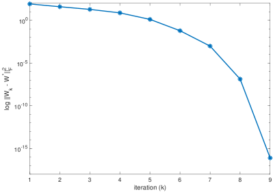
((a)) Convergence with exact learning

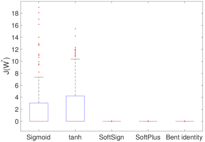
((b)) Impact of vanishing gradient

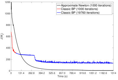
((c)) Convergence without exact learning

Figure 1: Investigation of an approximate Newton’s algorithm, a.k.a. the Generalised Gauss-Newton algorithm.

Remark 6.

The approximate Hessian proposed in Eq. (37) is by construction positive semi-definite at arbitrary weights, while definiteness of the exact Hessian is not conclusive. It is trivial to see that the approximate Hessian coincides with the ground-truth Hessian as Eq. (28) at global minima. Hence, when $\alpha=1$, the corresponding approximate Newton’s algorithm induced by the update rule in Eq. (40) shares the same local quadratic convergence properties to a global minimum as the exact Newton’s method (see Section 6).

In general, computing the approximate Newton’s update as defined in Eq. (38) can be computationally expensive. Interestingly, the approximate Newton’s algorithm is indeed the state of the art GGN algorithm developed in [29]. Efficient implementations of the GGN algorithm have been extensively explored in [30, 43, 44]. In the next section, we investigate the theoretical convergence properties of the approximate Newton’s algorithm, i.e., the GGN algorithm.

6 Numerical evaluation

In this section, we investigate performance of the Approximate Newton’s (AN) algorithm, i.e., the GGN algorithm. We test the algorithm on the four regions classification benchmark, as originally proposed in [45]. In $\mathbb{R}^{2}$ around the origin, we have a square area $(-4,4)\times(-4,4)$, and three concentric circles with their radiuses being $1$, $2$, and $3$. Four regions/classes are interlocked and nonconvex, see [45] for further details of the benchmark. Samples are drawn in the box for training with their corresponding outputs being the classes $\{1,2,3,4\}$.

We firstly demonstrate theoretical convergence properties of the AN/GGN algorithm with $\alpha=1$, by deploying an MLP architecture $\bm{\mathcal{F}}(2,20,1)$. Dummy units are introduced in both the input and hidden layer. Activation functions in the hidden layer are chosen to be the Bend identity, and the error function is the squared loss. With a set of $20$ randomly drawn training samples, we run the AN/GGN algorithm from randomly initialised weights. The convergence is measured by the distance of the accumulation point $\mathbf{W}^{*}$ to all iterates $\mathbf{W}^{(k)}$, i.e., by an extension of the Frobenius norm of matrices to collections of matrices as $\|\mathbf{W}^{(k)}-\mathbf{W}^{*}\|_{F}:=\sum_{l=1}^{L}\|W_{l}^{(k)}-W_{l}^{*}\|_{F}$. It is clear from Figure 1(a) that the AN/GGN algorithm converges locally quadratically fast to a global minimiser of exact learning.

We further investigate the performance of AN/GGN with five different activations, namely Sigmoid, $\operatorname{tanh}$, SoftSign, SoftPlus, and Bent identity. The first three activation functions are squashing, while the SoftPlus is only bounded from below, and the Bent identity is totally unbounded. Figure 1(b) gives the box plot of the value of the total loss function $\mathcal{J}$ over $100$ independent runs from random initialisations after convergence. Clearly, AN/GGNs with SoftPlus and Bent identity perform very well, while the ones with Sigmoid and $\operatorname{tanh}$ suffer from numerically spurious local minima. However, it is also very interesting to observe that SoftSign does not share the bad convergence behaviour as its squashing counterparts, due to some unknown factors.

Finally, we investigate the AN/GGN algorithm, comparing with the classic BP algorithm in terms of convergence speed, without exact learning being assumed. In this experiment, we adopt an MLP architecture $\bm{\mathcal{F}}(2,10,10,4)$, where the target outputs being the corresponding standard basis vector in $\mathbb{R}^{4}$, and the set step size to be constant $\alpha=0.01$. For running $1000$ iterations, the BP algorithm took $61.1$ sec., while the AN/GGN algorithm spent $1314.1$ sec. On average, the running time for each iteration of AN/GGN was about $21.4$ times as required for an iteration of BP. With the same data and the same random initialisation, we ran BP for $20760$ iterations, which took the same amount of time as required for $1000$ iterations of AN/GGN. As shown in Figure 1(c), the first $1000$ iterations of BP was highlighted in red with the remaining iterations being coloured in blue. The AN/GGN goes up at the beginning, then smoothly converges to the global minimal value, while the BP demonstrates strong oscillation towards the end.

7 Conclusion

In this work, we provide a smooth optimisation perspective on the challenge of training MLPs. Under the condition of exact learning, we characterise the critical point conditions of the empirical total loss function, and investigate sufficient conditions to ensure any local minimum to be globally minimal. Classic results on MLPs with only one hidden layer are reexamined in the proposed framework. Finally, the so-called Generalised Gauss-Newton algorithm is rigorously revisited as an approximate Newton’s algorithm, which shares the property of being locally quadratically convergent to a global minimum. All aspects discussed in this paper require a further systematic and thorough investigation both theoretically and experimentally, and are expected to be also applicable for training recurrent neural networks.

Appendix A Tracy-Singh product and Khatri-Rao product

Given two matrices $\mathbf{A}\in\mathbb{R}^{m\times n}$ and $\mathbf{B}\in\mathbb{R}^{p\times q}$. Let us partition $\mathbf{A}$ into blocks $A_{ij}\in\mathbb{R}^{m_{i}\times n_{j}}$, and $\mathbf{B}$ into blocks $B_{kl}\in\mathbb{R}^{p_{k}\times q_{l}}$. The Tracy-Singh product of $\mathbf{A}$ and $\mathbf{B}$ [46] is defined as

$$\mathbf{A}\circledast\mathbf{B}=(A_{ij}\circledast\mathbf{B})_{ij}=((A_{ij}\otimes B_{kl})_{kl})_{ij},$$ (41)

where the notion $(\cdot)_{ij}$ follows the convention of referring to the $(i,j)$-th block of a partitioned matrix. The matrix $\mathbf{A}\circledast\mathbf{B}$ is of the dimension $(mp)\times(nq)$, and its rank shares the same property as the Kronecker product of matrices as

$$\operatorname{rank}(\mathbf{A}\circledast\mathbf{B})=\operatorname{rank}(\mathbf{A})\operatorname{rank}(\mathbf{B}).$$ (42)

If $\mathbf{A}$ and $\mathbf{B}$ are partitioned identically, then the Khatri-Rao product of the two matrices is defined as

$$\mathbf{A}\odot\mathbf{B}=(A_{ij}\otimes B_{ij})_{ij}.$$ (43)

The matrix $\mathbf{A}\odot\mathbf{B}$ is of the dimension $(\sum_{i}\!m_{i}p_{i})\times(\sum_{i}\!n_{i}q_{i})$. The connection between the Tracy-Singh product and the Khatri-Rao product is given as

$$\mathbf{A}\odot\mathbf{B}=Z_{1}^{\top}(\mathbf{A}\circledast\mathbf{B})Z_{2},$$ (44)

where $Z_{1}\!\in\!\mathbb{R}^{(mp)\times(\sum_{i}\!m_{i}p_{i})}$ and $Z_{2}\!\in\!\mathbb{R}^{(nq)\times(\sum_{i}\!n_{i}q_{i})}$ are two selection matrices, satisfying $Z_{1}^{\top}Z_{1}=I_{\sum_{i}\!m_{i}p_{i}}$ and $Z_{2}^{\top}Z_{2}=I_{\sum_{i}\!n_{i}q_{i}}$. We refer to [47] for concrete constructions of matrices $Z_{1}$ and $Z_{2}$, and more technical details regarding the Khatri-Rao product. It is then trivial to conclude the following corollary.

Corollary 1.

Given two identically partitioned matrices $\mathbf{A}$ and $\mathbf{B}$, the rank of the Tracy-Singh product and the rank of the Khatri-Rao product of both matrices fulfils the following inequality

$$\operatorname{rank}(\mathbf{A}\odot\mathbf{B})\leq\operatorname{rank}(\mathbf{A}\circledast\mathbf{B}).$$ (45)

Furthermore, it is clear that

$$\operatorname{rank}(Z_{1})=\sum_{i}\!m_{i}p_{i},$$ (46)

and

$$\operatorname{rank}(Z_{2})=\sum_{i}\!n_{i}q_{i}.$$ (47)

Now, we recall the Frobenius’ rank inequality [41], i.e., given three matrices $A$, $B$, $C$ that have compatible dimensions, then

$$\operatorname{rank}(ABC)+\operatorname{rank}(B)\geq\operatorname{rank}(AB)+\operatorname{rank}(BC).\!$$ (48)

A special case of the Frobenius’ rank inequality is the so-called Sylvester’s rank inequality, i.e., given two matrices $A\in\mathbb{R}^{m\times n}$ and $C\in\mathbb{R}^{n\times p}$, then the rank of the product of $U$ and $V$ is bounded by

$$\operatorname{rank}(AC)\geq\operatorname{rank}(A)+\operatorname{rank}(C)-n.$$ (49)

Let $A\in\mathbb{R}^{m\times n_{1}}$, $B\in\mathbb{R}^{n_{1}\times n_{2}}$, and $C\in\mathbb{R}^{n_{2}\times p}$. By combining both the Frobenius’ rank inequality and the Sylvester’s rank inequality, we have

$$\begin{split}\operatorname{rank}(ABC)\geq&~{}\!\operatorname{rank}(AB)+\operatorname{rank}(BC)-\operatorname{rank}(B)\!\\ \geq&~{}\!\operatorname{rank}(A)+\operatorname{rank}(B)-n_{1}+\operatorname{rank}(B)+\operatorname{rank}(C)-n_{2}~{}-\\ &-\operatorname{rank}(B)\\ =&~{}\!\operatorname{rank}(A)+\operatorname{rank}(B)+\operatorname{rank}(C)-n_{1}-n_{2}.\end{split}$$ (50)

If the Tracy-Singh product $\mathbf{A}\circledast\mathbf{B}$ has full rank, denoted by

$$R_{ts}:=\operatorname{rank}(\mathbf{A}\circledast\mathbf{B}),$$ (51)

then the rank of the Khatri-Rao product $\mathbf{A}\odot\mathbf{B}$ is bounded from below by

$$\begin{split}\operatorname{rank}(\mathbf{A}\odot\mathbf{B})\geq&\sum_{i}\!m_{i}p_{i}+R_{ts}+\sum_{j}\!n_{j}q_{j}-mp-nq.\end{split}$$ (52)

Note, that the above lower bound is not guaranteed to be positive. Hence, nothing is conclusive about the rank of the Khatri-Rao product of two arbitrary full rank matrices.

Appendix B Proof of Proposition 2

Proof.

We can trivially rewrite the Kronecker product for each partition as

$$\begin{split}\Psi_{i}\otimes\phi_{i}=&~{}(I_{n_{l}}\Psi_{i})\otimes(\phi_{i}1)\\[1.42262pt] =&~{}(I_{n_{l}}\otimes\phi_{i})\Psi_{i}.\end{split}$$ (53)

Then, the Khatri-Rao product of $\mathbf{\Psi}$ and $\mathbf{\Phi}$ can be computed as the product of two matrices, i.e.,

$$\mathbf{\Psi}\odot\mathbf{\Phi}\!=\!\!\!\!\underbrace{[I_{n_{l}}\!\otimes\!\phi_{1},\ldots,I_{n_{l}}\!\otimes\!\phi_{T}]}_{=:(I_{n_{l}}\circledast\mathbf{\Phi})\in\mathbb{R}^{(n_{l}n_{n-1})\times(n_{l}T)}}\!\underbrace{\operatorname{diag}(\Psi_{1},\ldots,\Psi_{T})}_{=:\widetilde{\mathbf{\Psi}}\in\mathbb{R}^{(n_{l}T)\times(n_{L}T)}},\!$$ (54)

where $I_{n_{l}}\circledast\mathbf{\Phi}$ denotes the Tracy-Singh product of the identity matrix $I_{n_{l}}$ and $T$ column-wised partitioned matrix $\mathbf{\Phi}$, and the operator $\operatorname{diag}(\cdot)$ puts a sequence of matrices into a block diagonal matrix. By the rank property of the Tracy-Singh product, the rank of matrix $I_{n_{l}}\circledast\mathbf{\Phi}$ is equal to $n_{l}\operatorname{rank}(\mathbf{\Phi})$. Further, by the Sylvester’s rank inequality, the rank of $\mathbf{\Psi}\odot\mathbf{\Phi}$ is bounded from below

$$\operatorname{rank}(\mathbf{\Psi}\odot\mathbf{\Phi})\geq n_{l}\operatorname{rank}(\mathbf{\Phi})+\sum\limits_{i=1}^{T}\operatorname{rank}(\Psi_{i})-Tn_{L}.$$ (55)

Specifically, if all matrices $\Psi_{i}$’s and $\mathbf{\Phi}$ are of full rank, we have the following properties.

1. If $n_{l}\leq n_{L}$, then the rank of the block diagonal matrix $\widetilde{\mathbf{\Psi}}$ is equal to $n_{l}T$. By the Sylvester’s rank inequality [41], we have

   $$\begin{split}\operatorname{rank}(\mathbf{\Psi}\odot\mathbf{\Phi})\geq&~{}n_{l}\operatorname{rank}(\mathbf{\Phi})+n_{l}T-n_{l}T\\ =&~{}n_{l}\operatorname{rank}(\mathbf{\Phi}).\end{split}$$ (56)

2. If $n_{l}>n_{L}$ and $n_{l-1}\geq T$, then the rank of $\widetilde{\mathbf{\Psi}}$ is equal to $n_{L}T$, and the rank of $(I_{n_{l}}\circledast\mathbf{\Phi})$ is equal to $n_{l}T$. By the Sylvester’s rank inequality, we have

   $$\begin{split}\operatorname{rank}(\mathbf{\Psi}\odot\mathbf{\Phi})\geq&~{}n_{l}T+n_{L}T-n_{l}T\\ =&~{}n_{L}T.\end{split}$$ (57)

3. If $n_{l}>n_{L}$ and $n_{l-1}<T$, then the rank of $(I_{n_{l}}\circledast\mathbf{\Phi})$ is equal to $n_{l}n_{l-1}$. By the same argument, we have

   $$\operatorname{rank}(\mathbf{\Psi}\odot\mathbf{\Phi})\geq n_{l}n_{l-1}+n_{L}T-n_{l}T.$$ (58)

   It is clear that such a lower bound can be even negative, i.e., practically useless. However, since matrix $\mathbf{\Phi}$ is of full rank, there must exist a non-zero vector $\phi_{i}$, so that $\operatorname{rank}(\Psi_{i}\otimes\phi_{i})=n_{L}$. Then we have the result $\operatorname{rank}(\mathbf{\Psi}\odot\mathbf{\Phi})\geq n_{L}$.

∎

Appendix C Proof of Proposition 3

Proof.

By stacking all row blocks $\mathbf{\Psi}_{l}\odot\mathbf{\Phi}_{l-1}$ for $l=1,\ldots,L$ together, we have $\mathbf{P}(\mathbf{W})$ as in Eq. (22). We can rewrite $\mathbf{P}(\mathbf{W})$ as

$$\begin{split}\mathbf{P}(\mathbf{W})=&\operatorname{diag}\big{(}I_{n_{1}}\!\!\circledast\!\mathbf{\Phi}_{0},\ldots,I_{n_{L}}\!\!\circledast\!\mathbf{\Phi}_{L-1}\big{)}\cdot\operatorname{diag}\big{(}\widetilde{\mathbf{\Psi}}_{1},\ldots,\widetilde{\mathbf{\Psi}}_{L}\big{)}\cdot\mathbf{I}_{Tn_{l}}^{L},\end{split}$$ (59)

where $\mathbf{I}_{Tn_{l}}^{L}:=[I_{Tn_{L}},\ldots,I_{Tn_{L}}]^{\top}\in\mathbb{R}^{LTn_{L}\times Tn_{L}}$ is a matrix of stacking $L$ copies of the identity matrix $I_{Tn_{L}}$ on top of each other. Then, by applying Eq. (50), it is straightforward to get

$$\begin{split}\operatorname{rank}\!\big{(}\mathbf{P}(\mathbf{W})\big{)}\geq&\sum\limits_{l=1}^{L}n_{l}\operatorname{rank}\big{(}\mathbf{\Phi}_{l-1}\big{)}+\sum\limits_{l=1}^{L}\sum\limits_{i=1}^{T}\operatorname{rank}\big{(}\Psi_{l}^{(i)}\big{)}+Tn_{L}~{}-\\ &-\sum\limits_{l=1}^{L}Tn_{l}-LTn_{L}.\end{split}$$ (60)

The result follows directly. ∎

It is clear that such a bound in Proposition 3 is still very problem-dependent, and hard to control. Nevertheless, due to the special structure of $\mathbf{I}_{Tn_{l}}^{L}$, the actual rank bound is given practically by the largest bound of each individual row block as characterised in Proposition 2, i.e.,

$$\operatorname{rank}\!\big{(}\mathbf{P}(\mathbf{W})\big{)}\geq\max_{1\leq l\leq L}\operatorname{rank}\big{(}\mathbf{\Psi}_{l}\odot\mathbf{\Phi}_{l-1}\big{)}.$$ (61)

Appendix D Proof of Proposition 5

Proof.

We feed samples $X:=[x_{1},\ldots,x_{T}]\in\mathbb{R}^{n_{0}\times T}$ through the MLP to generate the outputs in the hidden layer $\Phi_{1}:=[\phi_{1}^{(1)},\ldots,\phi_{1}^{T}]\in\mathbb{R}^{T\times T}$, which is invertible due to Condition (2). It can be achieved by employing appropriate activation functions as suggested in [38], such as the Sigmoid and the $\operatorname{tanh}$. Then in the output layer, we have $\Phi_{2}:=[\phi_{2}^{(1)},\ldots,\phi_{2}^{(T)}]=W_{2}^{\top}\Phi_{1}\in\mathbb{R}^{n_{2}\times T}$. Let us denote by $Y:=[g^{*}(x_{1}),\ldots,g^{*}(x_{T})]\in\mathbb{R}^{n_{2}\times T}$ the desired outputs. Then, every pair $(W_{1},(Y\Phi_{1}^{-1})^{\top})$ is a global minimum of the total loss function.

We then compute the critical point conditions in the output layer as

$$\underbrace{\!\left[\!\!\!\begin{array}[]{ccc}I_{n_{2}}\!\otimes\phi_{1}^{(1)}&\!\!\!\!\!\ldots\!\!\!\!\!&I_{n_{2}}\!\otimes\phi_{1}^{(T)}\end{array}\!\!\!\right]\!}_{:=P_{2}\in\mathbb{R}^{(Tn_{2})\times(Tn_{2})}}\left[\!\!\!\begin{array}[]{c}\nabla_{\!E}(\phi_{2}^{(1)})\\ \vdots\\ \nabla_{\!E}(\phi_{2}^{(T)})\end{array}\!\!\!\right]\!=0,$$ (62)

where $P_{2}$ is a square matrix. By following case (1) in Proposition 2, we get $\operatorname{rank}(P_{2})=Tn_{2}$. The result simply follows. ∎

Note, that in Proposition 5, we do not consider the dummy units introduced by the scalar-valued bias $b_{l,k}$. Nevertheless, using similar arguments, the statements in Proposition 5 also hold true for the case with free variables $b_{l,k}$.

Appendix E Proof of Proposition 6

Proof.

It is straightforward to have

$$\begin{split}\operatorname{rank}\!\big{(}\mathbf{P}(\mathbf{W})\big{)}\geq&~{}n_{1}\operatorname{rank}\big{(}\mathbf{\Phi}_{0}\big{)}+n_{2}n_{1}-Tn_{1}+2Tn_{2}-2Tn_{2}\\ =&~{}n_{1}\big{(}\operatorname{rank}\big{(}\mathbf{\Phi}_{0}\big{)}+n_{2}-T\big{)}.\end{split}$$ (63)

Proposition 2 implies

$$\operatorname{rank}(\mathbf{\Psi}_{2}\odot\mathbf{\Phi}_{1})\geq n_{2}\operatorname{rank}(\mathbf{\Phi}_{1}),$$ (64)

and

$$\operatorname{rank}(\mathbf{\Psi}_{1}\odot\mathbf{\Phi}_{0})\geq n_{2}.$$ (65)

By the construction of $\operatorname{rank}(\mathbf{\Phi}_{1})\geq n_{1}$, the result follows directly. ∎

References

• [1] C. M. Bishop, Neural Networks for Pattern Recognition.   Oxford University Press, USA, 1996.
• [2] Y. LeCun, Y. Bengio, and G. Hinton, “Deep learning,” Nature, vol. 521, pp. 436–444, 2015.
• [3] D. Yu and L. Deng, Automatic Speech Recognition: A Deep Learning Approach.   Springer-Verlag, London, 2015.
• [4] X. Glorot and Y. Bengio, “Understanding the difficulty of training deep feedforward neural networks,” in Proceedings of the $13^{th}$ International Conference on Artificial Intelligence and Statistics (AISTATS), vol. 9, 2010, pp. 249–256.
• [5] K. Hornik, “Approximation capabilities of multilayer feedforward networks,” Neural Networks, vol. 4, no. 2, pp. 251–257, 1991.
• [6] S. Sun, W. Chen, L. Wang, X. Liu, and T.-Y. Liu, “On the depth of deep neural networks: A theoretical view,” in Proceedings of the $31^{st}$ AAAI Conference on Artificial Intelligence, 2016, pp. 2066–2072.
• [7] H. N. Mhaskar and C. A. Micchelli, “How to choose an activation function,” in Proceedings of the 6th International Conference on Neural Information Processing Systems, 1993, pp. 319–326.
• [8] T. Falas and A. G. Stafylopatis, “The impact of the error function selection in neural network-based classifiers,” in Proceedings of the International Joint Conference on Neural Networks (IJCNN), vol. 3, 1999, pp. 1799–1804.
• [9] B. Widrow and M. A. Lehr, “30 years of adaptive neural networks: perceptron, madaline, and backpropagation,” Proceedings of the IEEE, vol. 78, no. 9, pp. 1415–1442, 1990.
• [10] R. S. Sutton, “Two problems with backpropagation and other steepest-descent learning procedures for networks,” in Proceedings of the $8$-th Annual Conference of the Cognitive Science Society, 1986, pp. 823–831.
• [11] R. Rojas, Neural Networks: A Systematic Introduction.   Springer, 1996.
• [12] L. G. C. Hamey, “XOR has no local minima: A case study in neural network error surface analysis,” Neural Metworks, vol. 11, no. 4, pp. 669–681, 1998.
• [13] I. G. Sprinkhuizen-Kuyper and E. J. W. Boers, “The local minima of the error surface of the 2-2-1 XOR network,” Annals of Mathematics and Artificial Intelligence, vol. 25, no. 1, pp. 107–136, 1999.
• [14] A. Choromanska, M. Henaff, M. Mathieu, G. B. Arous, and Y. LeCun, “The loss surfaces of multilayer networks,” in Proceedings of the $18^{th}$ International Conference on Artificial Intelligence and Statistics (AISTATS), 2015, pp. 192–204.
• [15] P. J. G. Lisboa and S. J. Perantonis, “Complete solution of the local minima in the XOR problem,” Network: Computation in Neural Systems, vol. 2, no. 1, pp. 119–124, 1991.
• [16] I. G. Sprinkhuizen-Kuyper and E. J. W. Boers, “A local minimum for the 2-3-1 XOR network,” IEEE Transactions on Neural Networks, vol. 10, no. 4, pp. 968–971, 1999.
• [17] M. Gori and A. Tesi, “On the problem of local minima in backpropagation,” IEEE Transactions on Pattern Analysis and Machine Intelligence, vol. 14, no. 1, pp. 76–86, 1992.
• [18] X.-H. Yu, “Can backpropagation error surface not have local minima,” IEEE Transactions on Neural Networks, vol. 3, no. 6, pp. 1019–1021, 1992.
• [19] X.-H. Yu and G.-A. Chen, “On the local minima free condition of backpropagation learning,” IEEE Transactions on Neural Networks, vol. 6, no. 5, pp. 1300–1303, 1995.
• [20] J. F. Kolen and J. B. Pollack, “Backpropagation is sensitive to initial conditions,” Complex Systems, vol. 4, no. 3, pp. 269–280, 1990.
• [21] I. J. Goodfellow, O. Vinyals, and A. M. Saxe, “Qualitatively characterizing neural network optimization problems,” Published at the $5^{th}$ International Conference on Learning Representations (ICLR). arXiv:1412.6544., 2015.
• [22] K. Kawaguchi, “Deep learning without poor local minima,” in Advances in Neural Information Processing Systems 29, D. D. Lee, M. Sugiyama, U. V. Luxburg, I. Guyon, and R. Garnett, Eds., 2016, pp. 586–594.
• [23] Q. Nguyen and M. Hein, “The loss surface of deep and wide neural networks,” in Proceedings of the $34^{th}$ International Conference on Machine Learning, 2017.
• [24] B. D. Haeffele and R. Vidal, “Global optimality in neural network training,” in Proceedings of the IEEE Conference on Computer Vision and Pattern Recognition (CVPR), 2017, pp. 7331 – 7339.
• [25] T. P. Vogl, J. K. Mangis, A. K. Rigler, W. T. Zink, and D. L. Alkon, “Accelerating the convergence of the back-propagation method,” Biological Cybernetics, vol. 59, no. 4, pp. 257–263, 1988.
• [26] C. Charalambous, “Conjugate gradient algorithm for efficient training of artificial neural networks,” IEE Proceedings G - Circuits, Devices and Systems, vol. 139, no. 3, pp. 301–310, 1992.
• [27] Q. Le, J. Ngiam, A. Coates, A. Lahiri, B. Prochnow, and A. Ng, “On optimization methods for deep learning,” Proceedings of international conference on Machine Learning, 2011.
• [28] D. P. Kingma and J. L. Ba, “Adam: a method for stochastic optimization,” in The $3$-rd International Conference on Learning Representations, 2015, pp. 1–13.
• [29] N. N. Schraudolph, “Fast curvature matrix-vector products for second-order gradient descent,” Neural Computation, vol. 14, pp. 1723 – 1738, 2002.
• [30] J. Martens, “Deep learning via Hessian-free optimization,” in Proceedings of the $27^{th}$ International Conference on Machine Learning (ICML), 2010, pp. 735–742.
• [31] O. Vinyals and D. Povey, “Krylov subspace descent for deep learning,” in Proceedings of the $15^{th}$ International Conference on Arti cial Intelligence and Statistics (AISTATS), vol. 22, 2012, pp. 1261–1268.
• [32] J. Martens, “New perspectives on the natural gradient method,” arXiv:1412.1193v8, 2014.
• [33] R. Battiti, “First- and second-order methods for learning: Between steepest descent and newton’s method,” Neural Computation, vol. 4, no. 2, pp. 141–166, 1992.
• [34] Y.-J. Wang and C.-T. Lin, “A second-order learning algorithm for multilayer networks based on block Hessian matrix,” Neural Networks, vol. 11, no. 9, pp. 1607–1622, 1998.
• [35] C. Bishop, “Exact calculation of the hessian matrix for the multilayer perceptron,” Neural Computation, vol. 4, no. 4, pp. 494–501, 1992.
• [36] E. Mizutani and S. E. Dreyfus, “Second-order stagewise backpropagation for hessian-matrix analyses and investigation of negative curvature,” Neural Networks, vol. 21, no. 2-3, pp. 193–203, 2008.
• [37] O. Güler, Foundations of Optimization.   Springer, 2010.
• [38] Y. Ito, “Nonlinearity creates linear independence,” Advances in Computational Mathematics, vol. 5, no. 1, pp. 189–203, 1996.
• [39] J. V. Shah and C.-S. Poon, “Linear independence of internal representations in multilayer perceptrons,” IEEE Transactions on Neural Networks, vol. 10, no. 1, pp. 10–18, 1999.
• [40] H. R. and A. Zisserman, Multiple View Geometry in Computer Vision.   Cambridge University Press, New York, 2004.
• [41] D. A. Simovici, Linear Algebra Tools for Data Mining.   World Scientific Publishing Company, 2012.
• [42] J. Milnor, Morse Theory.   Princeton University Press, 1963.
• [43] M. Fairbank and E. Alonso, “Efficient calculation of the Gauss-Newton approximation of the Hessian matrix in neural networks,” Neural Computation, vol. 24, no. 3, pp. 607–610, 2012.
• [44] A. Botev, H. Ritter, and D. Barber, “Practical gauss-newton optimisation for deep learning,” in Proceedings of the $34^{th}$ International Conference on Machine Learning, 2017.
• [45] S. Singhal and L. Wu, “Training multilayer perceptrons with the extended Kalman algorithm,” in Advances in Neural Information Processing Systems, 1989, pp. 133–140.
• [46] D. S. Tracy and R. P. Singh, “A new matrix product and its applications in partitioned matrices,” Statistica Neerlandica, vol. 26, pp. 143–157, 1972.
• [47] S. Liu, “Matrix results on the Khatri-Rao and Tracy-Singh products,” Linear Algebra and its Applications, vol. 289, no. 1, pp. 267–277, 1999.