Dynamical contribution to the heat conductivity in stochastic energy exchanges of locally confined gases

Abstract

We present a systematic computation of the heat conductivity of the Markov jump process modeling the energy exchanges in an array of locally confined hard spheres at the conduction threshold. Based on a variational formula [Sasada M 2016, Thermal conductivity for stochastic energy exchange models, arXiv:1611.08866], explicit upper bounds on the conductivity are derived, which exhibit a rapid power-law convergence towards an asymptotic value. We thereby conclude that the ratio of the heat conductivity to the energy exchange frequency deviates from its static contribution by a small negative correction, its dynamic contribution, evaluated to be $-0.000\,373$ in dimensionless units. This prediction is corroborated by kinetic Monte Carlo simulations which were substantially improved compared to earlier results.

1 Introduction

Understanding the transport properties of many-body dynamical systems remains one among statistical physics’ greatest challenges. Much effort has thus been devoted to deriving Fourier’s law of heat conduction starting from a microscopic setup. Drawing upon the analogy with the problem of diffusion in periodic billiard tables [1, 2, 3], high-dimensional billiard systems were proposed to investigate heat transport [4]. Such billiards, which can be considered intermediate between the gas of hard balls and the periodic Lorentz gas, are designed so as to prevent hard balls from changing positions in a periodic array of confining cells while letting them interact pairwise. In a regime of rare interactions, i.e. the limit such that the binary collisions transporting energy are much less frequent than energy-conserving wall collision events, it was argued that the dynamics of energy exchanges between neighbouring hard balls can be mapped onto a stochastic model [5, 6, 7, 8, 9, 10]. This limit is reached for a critical geometry of the billiard whereby the system undergoes a transition from thermal conductor to insulator. The stochastic model stemming from the separation of the two timescales near the critical geometry is a Markov jump process for the local energy variables, which lends itself to a systematic derivation of Fourier’s law. Thus the necessary spectral gap was obtained in reference [11]; see also reference [12]. These results ultimately make possible the actual determination of the coefficient of heat conductivity of the billiard model at the conduction threshold.

In our previous works [5, 6, 7, 8, 9], as well as in reference [13], it was shown that heat conductivity can be expressed in terms of the frequency of binary collisions responsible for energy exchanges. Moreover, numerical results and theoretical considerations led us to conjecture that the dimensionless ratio between the heat conductivity and the frequency of binary collisions should be equal to unity at the conductor to insulator threshold. However, recent work by Sasada [14], relying upon a transposition of Spohn’s variational formula for diffusion coefficients of stochastic lattice gases [15, 16] to the heat conductivity of stochastic energy exchange models, proved that this conjecture cannot hold; the heat conductivity is in fact the sum of two parts: the static contribution, which is identical, up to a unit length squared, to the energy exchange frequency, and the dynamic contribution, which, however small it turns out to be, is strictly negative. The variational formula, which is the main focus of this work, was initially derived by Varadhan [17] in the context of a non-gradient Ginzburg-Landau model at infinite temperature and has since developed into a cornerstone of the framework for analyzing non-gradient models; see e.g. reference [18].

In the present paper, we set out to demonstrate that an explicit calculation of the dimensionless ratio between the heat conductivity and the energy exchange frequency can be achieved using the variational formula. Our method relies on the use of multivariate polynomial test functions of increasing number of variables and degrees to compute explicit upper bounds on the heat conductivity. The rapid power-law convergence towards an asymptotic value yields a narrow confidence interval for this quantity.

The predicted value thus obtained is in fact within the error bounds of the (inconclusive) numerical findings reported in reference [8] and therefore calls for a careful revision of our kinetic Monte Carlo simulations and the procedure by which the measurement of the heat conductivity is performed so as to improve its precision and confirm our new findings. We thereby show that the negative dynamic contribution to the heat conductivity inferred from the variational formula is in agreement with the value obtained from kinetic Monte Carlo simulations. This result confirms Sasada’s conclusion [14] and provides a prediction of the heat conductivity accurate to within at least six significant digits.

The paper is organized as follows. In section 2, the characterization of heat transport in many-body billiard systems with caged hard balls is reviewed from both microscopic and macroscopic considerations in subsection 2.1. In subsection 2.2, its transposition to stochastic energy exchange systems at the mesoscopic level is given. Within this framework, the variational formula is established in section 3. In particular, the application of the method to the stochastic energy exchanges induced by locally confined hard spheres is discussed in subsection 3.2. In subsection 3.3, the implementation of the variational formula is described for bivariate trial functions. Its extension to multivariate trial functions and its extrapolation to infinite-dimensional functions are presented in subsection 3.4. A comparison of the results thus obtained with kinetic Monte Carlo simulations is established in section 4. Section 5 concludes the paper.

2 Energy transport in locally confined gases

2.1 From microscopic dynamics to macroscopic fields

In the models described in references [5, 6, 7, 8, 9], we considered the motion of hard $D$-dimensional balls, $D\geq 2$, on a periodic $d$-dimensional array of cells, $1\leq d\leq D$, undergoing elastic collisions with locally confining hard walls as well as among neighbours. While the choice of the values of these two dimensions is mostly a matter of convenience, the distinction between the two is important. Unless otherwise stated, we will assume $D=3$ and $d=1$.

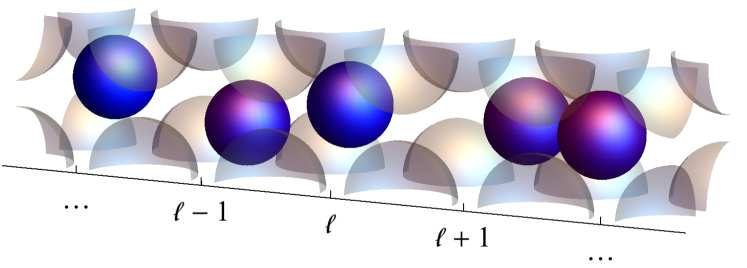
Figure 2.1: Schematic view of a billiard table composed of locally confined hard spheres. Mass transport is blocked by the geometry, but energy is transported through binary collisions among neighbouring hard balls, such as with the right-most pair.

Such a three-dimensional model on a one-dimensional lattice is schematically depicted in figure 2.1. In this example, identical hard spheres are randomly placed along a one-dimensional periodic array $\mathcal{L}_{N}=\{-(N-1)/2,\dots,(N-1)/2\}$ of $N$ small cavities composed of fixed spherical obstacles located at the corners of a cube of side $\ell$. To fix notations, we let the center of each cavity be located at $x_{l}=l\ell$. Each such cavity contains a single hard sphere which rattles around in it, unable to escape. The geometry is however chosen so as to allow neighbouring hard spheres to collide with each other.

In every cell, the motion of hard spheres is a succession of free flights interrupted by specular reflections which consist of two types of events: (i) wall collision events, through which a single ball reflects elastically off the spherical boundary of the cavity and does not change its energy, or (ii) binary collision events, which occur when two neighbouring balls collide with each other, thereby exchanging energy. The billiard geometry must verify specific conditions for such a regime to take place; see references [6, 9].

The system therefore consists in a gas of $N$ hard spheres whose spatial ordering is preserved by the dynamics. A current of energy may however be induced by the binary collision events, bringing about conduction of heat across the system.

For such a deterministic system, the local conservation of energy $\epsilon_{l}$ in cell $l=(l_{1},\dots,l_{d})$ can be expressed as

$$\dot{\epsilon}_{l}(t)=\sum_{i=1}^{d}\left[\mathcal{J}_{l-1_{i},l}(t)-\mathcal{J}_{l,l+1_{i}}(t)\right]\,,$$ (2.1)

in terms of the deterministic instantaneous currents $\mathcal{J}_{l,l+1_{i}}(t)$, where $1_{i}$ is the vector whose $d$ components are all $0$ but for the $i$^th which is $1$. In the case of billiards, these currents have the form

$$\mathcal{J}_{l,l+1_{i}}(t)=\sum_{n}\eta_{l,l+1_{i}}(t)\,\delta_{\mathrm{D}}(t-t^{(l,l+1_{i})}_{n})\,,$$ (2.2)

where $\eta_{l,l+1_{i}}(t)$ denotes the energy exchanged through the collision between balls in cells $l$ and $l+1_{i}$ at time $t$, $\{t^{(l,l+1_{i})}_{n}\}_{n\in\mathbb{N}}$ is the sequence of all successive collision times corresponding to binary collisions between balls $l$ and $l+1_{i}$ and the symbol $\delta_{\mathrm{D}}$ stands for the Dirac delta distribution. Integrating this quantity over time and summing over the lattice dimensions yields the kinetic energy of the $l^{\mathrm{th}}$ ball,

$$\epsilon_{l}(t)-\epsilon_{l}(0)=\sum_{i=1}^{d}\int_{0}^{t}\rmd t^{\prime}\left[\mathcal{J}_{l-1_{i},l}(t^{\prime})-\mathcal{J}_{l,l+1_{i}}(t^{\prime})\right]\,.$$ (2.3)

The connection with the macroscopic description is established by introducing the local temperature in terms of the kinetic energy averaged over some nonequilibrium statistical ensemble,

$$T(x_{l},t)=\frac{2}{D}\left\langle\epsilon_{l}(t)\right\rangle_{\textsc{neq}}\,,$$ (2.4)

where $\left\langle\cdot\right\rangle_{\textsc{neq}}$ denotes the time-dependent average with respect to the nonequilibrium statistical ensemble. Similarly, the local energy and energy current densities, with respect to cells of (hyper)cubic volume $\ell^{d}$ in a $d$-dimensional lattice, can be defined as

$$\begin{split}e(x_{l},t)&=\ell^{-d}\,\left\langle\epsilon_{l}(t)\right\rangle_{\textsc{neq}}\,,\\ j_{e,i}(x_{l},t)&=\ell^{-d+1}\,\tfrac{1}{2}\left\langle\mathcal{J}_{l-1_{i},l}(t)+\mathcal{J}_{l,l+1_{i}}(t)\right\rangle_{\textsc{neq}}\,,\end{split}$$ (2.5)

in terms of the deterministic currents (2.2). The heat capacity is thus given by

$$c=\frac{\partial e}{\partial T}=\frac{D}{2}\ell^{-d}\,,$$ (2.6)

under the assumption of local equilibrium.

If it exists, the heat conductivity enters at the macroscopic level, the expression of Fourier’s law, obtained in the hydrodynamic scaling limit where $\ell\to 0$,

$$j_{e}(x,t)=-\kappa(T(x,t))\,\mathrm{grad}\,T(x,t)\,,$$ (2.7)

where $j_{e}$ is the vector of components $j_{e,i}$, $i=1,\dots,d$, defined in equation (2.5). Moreover, since the energy current density $j_{e}$ obeys the local conservation law,

$$\partial_{t}\,e(x,t)+\mathrm{div}\,j_{e}(x,t)=0\,,$$ (2.8)

the heat equation can be written as

$$\partial_{t}T(x,t)=\mathrm{div}\left[\chi(T(x,t))\,\mathrm{grad}\,T(x,t)\right]\,,$$ (2.9)

in terms of the thermal diffusivity

$$\chi(T)=c^{-1}\kappa(T)=\frac{2\,\ell^{d}}{D}\,\kappa(T)\,.$$ (2.10)

The diffusivity and conductivity therefore differ in their units. Only the latter quantity will be referred to below.

In deterministic systems of $N$ balls with position coordinates $q_{l}$ and energies $\epsilon_{l}$ in a volume $V_{N}$, the heat conductivity is in general given by Helfand’s formula [19],

$$\kappa(T)=\lim_{t\to\infty}\lim_{N\to\infty}\frac{1}{2tV_{N}T^{2}}\left\langle\left[G(t)-G(0)\right]^{2}\right\rangle_{\textsc{eq}}\,,$$ (2.11)

where $G(t)=\sum_{l=1}^{N}q_{l}\,\epsilon_{l}$ is Helfand’s moment associated with energy, $\left\langle\cdot\right\rangle_{\textsc{eq}}$ denotes the average over the equilibrium statistical ensemble at the temperature $T$ and we assume the ratio $V_{N}/N$ is fixed as $N$ increases. For periodic arrays of cells of volume $\ell^{d}$, each containing a single ball, we have $V_{N}=N\ell^{d}$. Although the Green-Kubo formulation of the transport coefficients is often favoured over Helfand’s, the two are in fact equivalent; see reference [19].

In $(d=1)$-dimensional chains, such as depicted in figure 2.1, the confining geometry allows to simplify Helfand’s moment to

$$G(t)=\sum_{l\in\mathcal{L}_{N}}l\ell\,\epsilon_{l}(t)\,,$$ (2.12)

which holds irrespective of the spatial dimension $D$ of the underlying dynamics. For more general geometries, $\epsilon_{l}$ is to be interpreted as the energy associated with the gas (of one or more particles) trapped in cell $l$.

In the large system-size limit, using translation invariance of energy correlations and the local conservation of energy (2.1), it is possible to transform (2.11) with Helfand’s moment (2.12) to

$$\kappa(T)=-\frac{\ell}{4T^{2}}\lim_{t\to\infty}\frac{1}{t}\sum_{l\in\mathbb{Z}}l^{2}\left\langle\left[\epsilon_{l}(t)-\epsilon_{l}(0)\right]\left[\epsilon_{0}(t)-\epsilon_{0}(0)\right]\right\rangle_{\textsc{eq}}\,,$$ (2.13)

which applies to an infinite system; see also [14, equation (3.1)]. As explained in section 2.2, the contributions to this equation can be conveniently separated into static and dynamic correlations, so one can write

$$\kappa(T)\equiv\kappa_{\textsc{s}}(T)+\kappa_{\textsc{d}}(T)\,.$$ (2.14)

Whereas the static contribution, $\kappa_{\textsc{s}}(T)$, is easily computed, the dynamic contribution, $\kappa_{\textsc{d}}(T)$, is more elusive. Its computation will be the focus of section 3.

2.2 Mesoscopic description

As argued previously [5, 6, 7, 8, 9], the process of heat transport in the billiards described above reduces to a stochastic energy-exchange process in a regime of rare interactions, which occurs when the frequency of binary collisions is much smaller than the frequency of wall collisions. Whereas the former governs the timescale of energy exchanges, the latter randomizes the degrees of freedom not relevant to energy transport, i.e.  the positions and velocity directions. In other words, the separation between the two timescales induces averaging of these degrees of freedom.

Setting $d=1$, an energy configuration $\{\epsilon_{l}\}_{l\in\mathcal{L}_{N}}$ thus evolves according to a Markov jump process. On the one hand, the time evolution of the probability density $P\equiv P(\{\epsilon_{l}\}_{l\in\mathcal{L}_{N}},t)$ is specified by the master equation,

$$\partial_{t}P=\widehat{L}^{\dagger}\,P=\sum_{l\in\mathcal{L}_{N}}\widehat{L}_{l}^{\dagger}P\,,$$ (2.15)

with the local energy-exchange operator,

$$\widehat{L}_{l}^{\dagger}P(\dots,\epsilon_{l},\epsilon_{l+1},\dots)=\int_{-\epsilon_{l+1}}^{\epsilon_{l}}\rmd\eta\Big{[}W(\epsilon_{l}-\eta,\epsilon_{l+1}+\eta\,|\,\epsilon_{l},\epsilon_{l+1})\,P(\dots,\epsilon_{l}-\eta,\epsilon_{l+1}+\eta,\dots)\cr-W(\epsilon_{l},\epsilon_{l+1}\,|\,\epsilon_{l}-\eta,\epsilon_{l+1}+\eta)\,P(\dots,\epsilon_{l},\epsilon_{l+1},\dots)\Big{]},$$ (2.16)

whose structure is the usual difference between gain and loss terms, defined in terms of a stochastic kernel $W$ to be specified below. On the other hand, observables $A\equiv A(\{\epsilon_{l}\}_{l\in\mathcal{L}_{N}},t)$ evolve in time under the action of the adjoint operator, $\widehat{L}$, which takes the somewhat simpler form:

$$\partial_{t}A=\widehat{L}\,A=\sum_{l\in\mathcal{L}_{N}}\widehat{L}_{l}A\,,$$ (2.17)

with

$$\widehat{L}_{l}A(\dots,\epsilon_{l},\epsilon_{l+1},\dots)=\int_{-\epsilon_{l+1}}^{\epsilon_{l}}\rmd\eta\,W(\epsilon_{l},\epsilon_{l+1}|\epsilon_{l}-\eta,\epsilon_{l+1}+\eta)\cr\times\Big{[}A(\dots,\epsilon_{l}-\eta,\epsilon_{l+1}+\eta,\dots)-A(\dots,\epsilon_{l},\epsilon_{l+1},\dots)\Big{]}\,.$$ (2.18)

Assuming periodic boundary conditions, the terms $l=(N-1)/2$ in (2.15) and (2.17) couple the right-most cell $(N-1)/2$ with the left-most one $-(N-1)/2$.

For future reference, note that, in infinite-size systems, the natural equilibrium distribution for $D=3$ is the canonical probability distribution,

$$P_{\textsc{eq}}(\dots,\epsilon_{l},\epsilon_{l+1},\dots)=\prod_{l\in\mathcal{L}_{N}}\left[\frac{2\beta}{\sqrt{\pi}}\sqrt{\beta\epsilon_{l}}\,\rme^{-\beta\epsilon_{l}}\right].$$ (2.19)

For general $D$, it is given by the product of Gamma distributions of shape parameter $\tfrac{D}{2}$ and scale parameter specified by the temperature $T=\beta^{-1}$, such that $\lim_{N\to\infty}N^{-1}\sum_{l\in\mathcal{L}_{N}}\epsilon_{l}=\tfrac{D}{2}T$. This is a stationary solution of the master equation (2.15).

In this stochastic description, the local conservation of energy becomes

$$\partial_{t}\,\left\langle\epsilon_{l}\right\rangle_{\textsc{neq}}=\left\langle j(\epsilon_{l-1},\epsilon_{l})\right\rangle_{\textsc{neq}}-\left\langle j(\epsilon_{l},\epsilon_{l+1})\right\rangle_{\textsc{neq}}$$ (2.20)

where $\left\langle\cdot\right\rangle_{\textsc{neq}}$ now denotes the statistical average with respect to the time-dependent nonequilibrium probability distribution $P$ and the local average current is defined to be:

$$j(\epsilon_{l},\epsilon_{l+1})=\int\rmd\eta\,\eta\,W(\epsilon_{l},\epsilon_{l+1}|\epsilon_{l}-\eta,\epsilon_{l+1}+\eta)\,.$$ (2.21)

This observable is antisymmetric under the permutation of its arguments,

$$j(\epsilon_{l},\epsilon_{l+1})=-j(\epsilon_{l+1},\epsilon_{l})\,.$$ (2.22)

In the stochastic description, contrary to what equation (2.3) of the deterministic description would suggest, the change of energy at site $l$ in time $t$ is not simply given by the time integration of the local average currents (2.21). Rather, an additional contribution must be taken into consideration, given by a martingale $M_{l}(t)$,

$$\epsilon_{l}(t)-\epsilon_{l}(0)=M_{l}(t)+\int_{0}^{t}\rmd t^{\prime}j\left[\epsilon_{l-1}(t^{\prime}),\epsilon_{l}(t^{\prime})\right]-\int_{0}^{t}\rmd t^{\prime}j\left[\epsilon_{l}(t^{\prime}),\epsilon_{l+1}(t^{\prime})\right]\,.$$ (2.23)

In this expression the left-hand side is the exact change of energy at site $l$ in time $t$. The integrals on the right-hand side are, however, carried out over the currents (2.21), which correspond to averaged quantities. By contrast, the actual succession of random energy jumps in time $t$ displays fluctuations about these average currents. The martingale $M_{l}(t)$ thus represents the difference between the actual change of energy in time $t$ and the corresponding time integrals of the local average currents. Considering the differential of this expression, $\rmd\epsilon_{l}(t)=j\left[\epsilon_{l-1}(t),\epsilon_{l}(t)\right]\,\rmd t-j\left[\epsilon_{l}(t),\epsilon_{l+1}(t)\right]\,\rmd t+\rmd M_{l}(t)$, we see that $\rmd M_{l}(t)$ is akin to a Langevin noise term.

Since martingales have independent increments, $M_{l}$ satisfies the following property

$$\left\langle M_{l}(t)M_{0}(t)\right\rangle_{\textsc{eq}}=-2t\left\langle\epsilon_{l}\left[j(\epsilon_{-1},\epsilon_{0})-j(\epsilon_{0},\epsilon_{1})\right]\right\rangle_{\textsc{eq}};$$ (2.24)

see [14]. Solving equation (2.23) for $M_{l}(t)$, the left-hand side of equation (2.24) can be expressed in terms of the sum of three terms, one involving correlations between energy changes, as they appear on the right-hand side of equation (2.13), a second term involving correlations between energy changes and time-integrals of the local average currents, and a third one involving self-correlations of time-integrals of the local average currents. As pointed out by Spohn [15, 16], the equilibrium averages of the cross-terms between the change of the conserved quantity, given by the left-hand side of equation (2.23), and the time integral of the local average currents, as on the right-hand side of the same equation, must vanish because the former is odd under time reversal while the latter is even. Therefore, after summing (2.24) over $l\in\mathbb{Z}$ and transforming the correlation functions using translation invariance, we can multiply the resulting expression by $-\ell/(4T^{2}\,t)$ and take the limit $t\to\infty$, as in equation (2.13), to obtain the expression of the heat conductivity

$$\kappa(T)=\tfrac{1}{2}\ell\,T^{-2}\left\langle(\epsilon_{0}-\epsilon_{1})j(\epsilon_{0},\epsilon_{1})\right\rangle_{\textsc{eq}}-\ell\,T^{-2}\sum_{l\in\mathbb{Z}}\int_{0}^{\infty}\rmd t\left\langle j(\epsilon_{0},\epsilon_{1})\,\rme^{\widehat{L}t}j(\epsilon_{l},\epsilon_{l+1})\right\rangle_{\textsc{eq}},$$ (2.25)

where we recall $\widehat{L}=\sum_{l\in\mathbb{Z}}\widehat{L}_{l}$ is the time-evolution generator (2.17)-(2.18) for the observables. Remark here that a necessary condition for the time integral to converge is that $\widehat{L}$ be non-positive definite.

The first term on the right-hand side of equation (2.25) is identified as the static contribution to the heat conductivity in equation (2.14),

$$\kappa_{\textsc{s}}(T)=\tfrac{1}{2}\ell\,T^{-2}\left\langle(\epsilon_{0}-\epsilon_{1})j(\epsilon_{0},\epsilon_{1})\right\rangle_{\textsc{eq}}=\tfrac{1}{2}\ell\,T^{-2}\left\langle h(\epsilon_{0},\epsilon_{1})\right\rangle_{\textsc{eq}}=\ell\,\left\langle\nu(\epsilon_{0},\epsilon_{1})\right\rangle_{\textsc{eq}},$$ (2.26)

where

$$\nu(\epsilon_{0},\epsilon_{1}) =\int\rmd\eta\,W(\epsilon_{0},\epsilon_{1}|\epsilon_{0}-\eta,\epsilon_{1}+\eta)\,,$$ (2.27)

$$h(\epsilon_{0},\epsilon_{1}) =\int\rmd\eta\,\eta^{2}\,W(\epsilon_{0},\epsilon_{1}|\epsilon_{0}-\eta,\epsilon_{1}+\eta)\,,$$ (2.28)

are the zeroth and second moments of the stochastic kernel. The former is nothing but the mean frequency of binary collisions for the corresponding energy pair. The second term on the right-hand side of equation (2.25) is therefore identified as the dynamic contribution,

$$\kappa_{\textsc{d}}(T)=-\ell\,T^{-2}\sum_{l\in\mathbb{Z}}\int_{0}^{\infty}\rmd t\left\langle j(\epsilon_{0},\epsilon_{1})\,\rme^{\widehat{L}t}j(\epsilon_{l},\epsilon_{l+1})\right\rangle_{\textsc{eq}}\,.$$ (2.29)

Before we turn to the characterization of this second term in section 3, we note that one can formally write:

$$\int_{0}^{\infty}\rmd t\,\rme^{\widehat{L}t}=-\widehat{L}^{-1}\,,$$ (2.30)

which assumes the operator $\widehat{L}$ causes relaxation after long enough times. Accordingly, equation (2.25) can be rewritten as the statistical average of the heat current $j(\epsilon_{0},\epsilon_{1})$,

$$\kappa(T)=-\left\langle j(\epsilon_{0},\epsilon_{1})\,\Psi_{\textsc{{st}}}\right\rangle_{\textsc{eq}},$$ (2.31)

where

$$\Psi_{\textsc{{st}}}\equiv\Psi_{\textsc{{st}}}(\{\epsilon_{l}\}_{l\in\mathbb{Z}})=\tfrac{1}{2}\ell\,T^{-2}(\epsilon_{1}-\epsilon_{0})-\ell\,T^{-2}\sum_{l\in\mathbb{Z}}\widehat{L}^{-1}j(\epsilon_{l},\epsilon_{l+1})\,,$$ (2.32)

is an infinite-dimensional function to be interpreted in terms of the first-order expansion of a nonequilibrium steady state in powers of its local temperature gradient.

Indeed, consider the transposition of equation (2.7) to a nonequilibrium steady state with temperature profile $T(x_{l})$, $x_{l}=l\,\ell$, $l\in\mathcal{L}_{N}$, resulting from the presence of heat baths at different temperatures at the system boundaries. Assuming $N$ large, we have

$$\kappa(T(x_{l}))=-\left(\frac{\rmd T}{\rmd x_{l}}\right)^{-1}j_{e}(x_{l}),$$ (2.33)

where the macroscopic current $j_{e}(x_{l})$ should, in analogy with the second of equations (2.5), be expressed in terms of the symmetrized sum $\tfrac{1}{2}\left\langle j(\epsilon_{l-1},\epsilon_{l})+j(\epsilon_{l},\epsilon_{l+1})\right\rangle_{\textsc{neq}}$. Comparing with equation (2.31), we see that the two-cell marginal of $\Psi_{\textsc{{st}}}$,

$$\int\prod_{l\neq 0,\,1}\rmd\epsilon_{l}\Psi_{\textsc{{st}}}(\dots,\epsilon_{0},\epsilon_{1},\dots)\,,$$ (2.34)

can be identified as the coefficient of the first-order contribution in the local temperature gradient to the probability density of the nonequilibrium steady state with respect to the equilibrium state (2.19). To be more precise, it is the part of the nonequilibrium steady state which contributes to the current. This is, however, not to say that $\Psi_{\textsc{{st}}}$ fully accounts for the actual density of the nonequilibrium steady state.

3 Variational formula

3.1 General framework

As shown by Spohn in reference [16], a Hilbert space $\cal H$ can be introduced for complex functions $f,g$ of the variables $\{\epsilon_{l}\}_{l\in\mathbb{Z}}$ with the degenerate scalar product:

$$\langle f|g\rangle_{\mathcal{H}}\equiv\sum_{k\in\mathbb{Z}}\Big{(}\left\langle f^{\star}\widehat{\tau}^{k}g\right\rangle_{\textsc{eq}}-\left\langle f^{\star}\right\rangle_{\textsc{eq}}\left\langle g\right\rangle_{\textsc{eq}}\Big{)}\,,$$ (3.1)

where ^⋆ denotes the complex conjugation and $\widehat{\tau}^{k}$ is the translation operator by $k$ cells to the left, mapping $\{\epsilon_{l}\}_{l}$ onto $\{\epsilon^{\prime}_{l}=\epsilon_{l+k}\}_{l}$. This scalar product is well defined, i.e. the sum over $k$ converges, because the equilibrium distribution has the mixing property under the spatial translations $\{\widehat{\tau}^{k}\}_{k}$ [16]. Let $\widehat{L}$ also denote the extension of the operator (2.18) to this Hilbert space. It is proved in references [15, 16] that

$$\mathrm{inf}_{f}\Big{(}-\langle f|\widehat{L}f\rangle_{\mathcal{H}}-2\,\langle j|f\rangle_{\mathcal{H}}\Big{)}=\langle j|\widehat{L}^{-1}j\rangle_{\mathcal{H}}\,,$$ (3.2)

where the infimum can be taken over real functions $f$. This result is obtained by expanding the vectors and the operator in a complete basis of the Hilbert space and by taking the first variation with respect to the function $f$, which leads to

$$\langle\delta f|\widehat{L}f\rangle_{\mathcal{H}}+\langle\delta f|j\rangle_{\mathcal{H}}=0\,.$$ (3.3)

Formally, this implies that $|f\rangle_{\mathcal{H}}=-|\widehat{L}^{-1}j\rangle_{\mathcal{H}}$. Making this substitution in the left-hand side of equation (3.2), one obtains the right-hand side. The infimum is thus explicitly realized for the function

$$f_{\textsc{inf}}=-\sum_{k\in\mathbb{Z}}\widehat{L}^{-1}\widehat{\tau}^{k}j\,,$$ (3.4)

so that $\Psi_{\textsc{{st}}}$ in (2.32) can be written as

$$\Psi_{\textsc{{st}}}=\tfrac{1}{2}\ell\,T^{-2}(\epsilon_{1}-\epsilon_{0})+\ell\,T^{-2}f_{\textsc{inf}}\,.$$ (3.5)

Now, from equation (2.30), the dynamic contribution to the heat conductivity (2.29) can be expressed, in terms of the scalar product (3.1) and using $\left\langle j\right\rangle_{\textsc{eq}}\equiv 0$, as

$$\kappa_{\textsc{d}}(T) =\ell\,T^{-2}\sum_{k\in\mathbb{Z}}\left\langle j\,\widehat{L}^{-1}\widehat{\tau}^{k}\,j\right\rangle_{\textsc{eq}}\,,$$ (3.6)

$$=\ell\,T^{-2}\langle j|\widehat{L}^{-1}\,j\rangle_{\mathcal{H}}\,,$$ (3.7)

$$=\ell\,T^{-2}\mathrm{inf}_{f}\left(-\langle f|\widehat{L}f\rangle_{\mathcal{H}}-2\,\langle j|f\rangle_{\mathcal{H}}\right)\,,$$ (3.8)

where the last line follows from equation (3.2).

Using equation (2.18) and the detailed balance condition,

$$P_{\textsc{eq}}(...,\epsilon_{0},\epsilon_{1},...)W(\epsilon_{0},\epsilon_{1}|\epsilon_{0}-\eta,\epsilon_{1}+\eta)=P_{\textsc{eq}}(...,\epsilon_{0}-\eta,\epsilon_{1}+\eta,...)W(\epsilon_{0}-\eta,\epsilon_{1}+\eta|\epsilon_{0},\epsilon_{1})\,,$$ (3.9)

the two following identities are obtained for the quantities appearing on the left-hand side of equation (3.6):

$$-\langle f|\widehat{L}f\rangle_{\mathcal{H}} =\tfrac{1}{2}\left\langle\int\rmd\eta\,W(\epsilon_{0},\epsilon_{1}|\epsilon_{0}-\eta,\epsilon_{1}+\eta)\Big{(}\sum_{k\in\mathbb{Z}}D_{0,1,\eta}\widehat{\tau}^{k}f\Big{)}^{2}\right\rangle_{\textsc{eq}},$$ (3.10)

$$-2\langle j|f\rangle_{\mathcal{H}} =-2\left\langle j\sum_{k\in\mathbb{Z}}\widehat{\tau}^{k}f\right\rangle_{\textsc{eq}}\,,$$ (3.11)

$$=\left\langle\int\rmd\eta\,W(\epsilon_{0},\epsilon_{1}|\epsilon_{0}-\eta,\epsilon_{1}+\eta)\,\eta\,\sum_{k\in\mathbb{Z}}D_{0,1,\eta}\widehat{\tau}^{k}f\right\rangle_{\textsc{eq}},$$ (3.12)

where we introduced the exchange operator $D_{l,l+1,\eta}$, [16],

$$D_{l,l+1,\eta}f\equiv f(\dots,\epsilon_{l}-\eta,\epsilon_{l+1}+\eta,\dots)-f(\dots,\epsilon_{l},\epsilon_{l+1},\dots)\,,$$ (3.13)

which, by convention, is a function of the pair of indices $l$ and $l+1$ rather than the positions of the corresponding variables. We note that equation (3.10) further relies on the identity $\left\langle L_{l}f\right\rangle_{\textsc{eq}}=0$, itself a consequence of the detailed balance.

Combining these two results with equation (3.6) and the expression of the static contribution, equation (2.26), the heat conductivity (2.14) is finally expressed as the solution of the variational formula,

$$\kappa(T)=\frac{\ell}{2T^{2}}\,\mathrm{inf}_{f}\left\langle\int\rmd\eta\,W(\epsilon_{0},\epsilon_{1}|\epsilon_{0}-\eta,\epsilon_{1}+\eta)\Big{(}\eta+\sum_{k\in\mathbb{Z}}D_{0,1,\eta}\widehat{\tau}^{k}f\Big{)}^{2}\right\rangle_{\textsc{eq}}\,,$$ (3.14)

in agreement with Sasada [14, equation (A.1)]. Moreover, the probability density distribution of the nonequilibrium steady state contributing to the current is locally given by equation (3.5), in terms of the function realizing the infimum.

An important property is that the solutions (3.4) of the variational formula are defined up to functions of a single variable. Indeed, a function $\Delta f=\sum_{l}\varphi(\epsilon_{l})$ may always be added to the solution (3.4) without changing the value of the conductivity (2.31). This is so because the antisymmetry (2.22) of the local average current implies

$$\left\langle j(\epsilon_{0},\epsilon_{1})\sum_{l}\varphi(\epsilon_{l})\right\rangle_{\textsc{eq}} =\sum_{l\leq-1}\underbrace{\left\langle j(\epsilon_{0},\epsilon_{1})\right\rangle_{\textsc{eq}}}_{\,=\,0}\left\langle\varphi(\epsilon_{l})\right\rangle_{\textsc{eq}}+\left\langle j(\epsilon_{0},\epsilon_{1})\varphi(\epsilon_{0})\right\rangle_{\textsc{eq}}$$ (3.15)

$$\quad+\left\langle j(\epsilon_{0},\epsilon_{1})\varphi(\epsilon_{1})\right\rangle_{\textsc{eq}}+\sum_{2\leq l}\underbrace{\left\langle j(\epsilon_{0},\epsilon_{1})\right\rangle_{\textsc{eq}}}_{\,=\,0}\left\langle\varphi(\epsilon_{l})\right\rangle_{\textsc{eq}}\,,$$ (3.16)

$$=\left\langle j(\epsilon_{0},\epsilon_{1})\varphi(\epsilon_{0})\right\rangle_{\textsc{eq}}-\left\langle j(\epsilon_{1},\epsilon_{0})\varphi(\epsilon_{1})\right\rangle_{\textsc{eq}}\,,$$ (3.17)

$$=\left\langle j(\epsilon_{0},\epsilon_{1})\varphi(\epsilon_{0})\right\rangle_{\textsc{eq}}-\left\langle j(\epsilon_{0},\epsilon_{1})\varphi(\epsilon_{0})\right\rangle_{\textsc{eq}}\,,$$ (3.18)

$$=0\,.$$ (3.19)

Furthermore and by the same token, only antisymmetric functions of $\epsilon_{0}$ and $\epsilon_{1}$ can produce non-trivial contributions to the variational formula. Solutions (3.4) are therefore defined up to symmetric functions of these arguments.

3.2 Application to the stochastic energy exchanges of locally confined hard spheres

Stochastic kernel.

In order to reduce the problem to the calculation of dimensionless quantities at equilibrium, we set $\ell\equiv 1$ and rescale the stochastic kernel according to

$$W(\epsilon_{0},\epsilon_{1}|\epsilon_{0}-\eta,\epsilon_{1}+\eta)=\nu(T)\,\beta\,w(\beta\epsilon_{0},\beta\epsilon_{1}|\beta\epsilon_{0}-\beta\eta,\beta\epsilon_{1}+\beta\eta)\,,$$ (3.20)

in terms of the inverse temperature $\beta=T^{-1}$ and the corresponding equilibrium average of the binary collision frequency (2.27),

$$\nu(T)=\left\langle\nu(\epsilon_{0},\epsilon_{1})\right\rangle_{\textsc{eq}}\equiv\sqrt{T}\,,$$ (3.21)

which now has the dimensions of the heat conductivity. Notice the second equality can be assumed without loss of generality, under a proper rescaling of time; see reference [8, Section 6].

Introducing the dimensionless quantities $e_{l}\equiv\beta\,\epsilon_{l}$ and $h\equiv\beta\,\eta$, the rescaled stochastic kernel for a system of hard spheres ($D=3$) can be written out as

$$w(e_{0},e_{1}|e_{0}-h,e_{1}+h)=\frac{1}{(2\pi)^{3/2}\sqrt{e_{0}\,e_{1}}}\int_{\mathbf{n}_{01}\cdot\mathbf{u}_{01}>0}\rmd\mathbf{u}_{0}\,\rmd\mathbf{u}_{1}\,\mathbf{n}_{01}\cdot\mathbf{u}_{01}\,\delta_{\mathrm{D}}(e_{0}-\mathbf{u}_{0}^{2})\cr\times\delta_{\mathrm{D}}(e_{1}-\mathbf{u}_{1}^{2})\,\delta_{\mathrm{D}}\left[h-(\mathbf{n}_{01}\cdot\mathbf{u}_{0})^{2}+(\mathbf{n}_{01}\cdot\mathbf{u}_{1})^{2}\right],$$ (3.22)

where $\mathbf{u}_{01}=\mathbf{u}_{0}-\mathbf{u}_{1}$ is proportional to the relative velocity between the two colliding balls and $\mathbf{n}_{01}$ is a three-dimensional unit vector joining the centers of the balls $0$ and $1$. The explicit form of the stochastic kernel is given by

$$w(e_{0},e_{1}|e_{0}-h,e_{1}+h)=\sqrt{\frac{\pi}{8}}\times\begin{cases}\sqrt{\frac{e_{1}+h}{e_{0}\,e_{1}}}\,,&-e_{1}<h<\mathrm{min}(0,e_{0}-e_{1})\,,\\ \frac{1}{\sqrt{\mathrm{max}(e_{0},e_{1})}}\,,&\mathrm{min}(0,e_{0}-e_{1})<h<\mathrm{max}(0,e_{0}-e_{1})\,,\\ \sqrt{\frac{e_{0}-h}{e_{0}\,e_{1}}}\,,&\mathrm{max}(0,e_{0}-e_{1})<h<e_{0}\,,\end{cases}$$ (3.23)

and zero otherwise. Equations (2.27)-(2.28) become

$$\nu(e_{0},e_{1}) =\frac{\sqrt{2\pi}}{12}\frac{e_{0}+e_{1}+2\,\mathrm{max}(e_{0},e_{1})}{\mathrm{max}({e_{0}},{e_{1}})^{1/2}}\,,$$ (3.24)

$$h(e_{0},e_{1}) =\frac{\sqrt{2\pi}}{420}\frac{11(e_{0}^{3}+e_{1}^{3})+7\,e_{0}\,e_{1}[3(e_{0}+e_{1})-8\,\mathrm{max}(e_{0},e_{1})]+24\,\mathrm{max}(e_{0},e_{1})^{3}}{\mathrm{max}({e_{0}},{e_{1}})^{1/2}}\,,$$ (3.25)

with the associated current (2.21),

$$j(e_{0},e_{1})=\tfrac{1}{2}(e_{0}-e_{1})\nu(e_{0},e_{1})\,;$$ (3.26)

see reference [8].

We note that the stochastic kernel is both symmetric with respect to space inversion and time reversal (or detailed balance):

$$\begin{split}&w(e_{0},e_{1}|e_{0}-h,e_{1}+h)=w(e_{1},e_{0}|e_{1}+h,e_{0}-h)\,,\\ &\sqrt{e_{0}\,e_{1}}\,w(e_{0},e_{1}|e_{0}-h,e_{1}+h)=\sqrt{(e_{0}-h)(e_{1}+h)}\,w(e_{0}-h,e_{1}+h|e_{0},e_{1})\,.\end{split}$$ (3.27)

Implementation of the variational formula.

In terms of the dimensionless stochastic kernel introduced in equation (3.20), the variational formula (3.14) reads

$$\kappa(T)=\tfrac{1}{2}\sqrt{T}\,\mathrm{inf}_{f}\left\langle\int dh\,w(e_{0},e_{1}|e_{0}-h,e_{1}+h)\Big{(}h+\sum_{k\in\mathbb{Z}}D_{0,1,h}\widehat{\tau}^{k}f\Big{)}^{2}\right\rangle_{\textsc{eq}}.$$ (3.28)

Trial functions $f$ can be expanded in terms of the generalized Laguerre polynomials $L_{n}^{({1}/{2})}(x)$, which form an orthogonal basis:

$$\int_{0}^{\infty}dx\,\sqrt{x}\,\rme^{-x}\,L_{m}^{({1}/{2})}(x)\,L_{n}^{({1}/{2})}(x)=\frac{1}{n!}\,\Gamma(n+3/2)\,\delta_{m,n}\,,$$ (3.29)

where $\delta_{m,n}$ denotes the Kronecker symbol and the Gamma function of half-integer argument can be expressed as

$$\Gamma(n+3/2)=\sqrt{\pi}\,\frac{(2n+1)!!}{2^{n+1}}\,.$$ (3.30)

It is convenient to define a basis of orthonormal functions

$$J_{n}(x)=\sqrt{\frac{2^{n}\,n!}{(2n+1)!!}}\,L_{n}^{({1}/{2})}(x)\,,$$ (3.31)

which satisfy the orthonormality condition

$$\frac{2}{\sqrt{\pi}}\int_{0}^{\infty}dx\,\sqrt{x}\rme^{-x}\,J_{m}(x)\,J_{n}(x)=\delta_{m,n}\,,$$ (3.32)

with weight function given by a Gamma distribution of shape parameter $\tfrac{3}{2}$ and scale parameter unity (which coincides with the single-cell marginal of the equilibrium distribution (2.19) at unit temperature).

To find the infimum of the variational formula (3.28), trial functions with an increasing number $r$ of variables can be successively considered:

$$f(e_{1},\dots,e_{r})=\sum_{n_{1},\dots,n_{r}}\gamma^{(r,\,\infty)}_{n_{1},\dots,n_{r}}\,J_{n_{1}}(e_{1})\dots J_{n_{r}}(e_{r})\,.$$ (3.33)

We refer to the number of variables $r$ as the order of the approximation. Functions of order $r=2$ are obviously a subset of functions of order $r\geq 3$ and similarly for every $r$.

The $\infty$ superscript on the coefficients appearing in equation (3.33) refers to the unrestricted sum over $n_{i}\in\mathbb{N}$, $i=1,\dots,r$. That is, for a fixed order $r$, the sum in equation (3.33) runs over orthonormal Laguerre polynomials of all degrees. By restricting this sum to a maximum degree $s$, such that $n_{1}+\dots+n_{r}\leq s$, we obtain a function space of finite dimension for which the variational formula boils down to computing the infimum of a quadratic form in the coefficients $\gamma^{(r,\,s)}_{n_{1},\dots,n_{r}}$. Its solution thus yields an approximation, $\kappa_{\textsc{d}}^{(r,\,s)}$, to the actual dynamical contribution to the heat conductivity in the form of an upper bound,

$$\kappa_{\textsc{d}}<\kappa_{\textsc{d}}^{(r,\,s)}\,,$$ (3.34)

obtained by restricting the computation of the infimum in (3.28) to the set of multivariate polynomials of $r$ variables and degree $s$.

For every order $r$, the optimal upper bound, $\kappa_{\textsc{d}}^{(r,\,\infty)}$, is obtained by letting $s\to\infty$. The convergence to the actual infimum is subsequently obtained by letting $r\to\infty$. The dynamical contribution to the heat conductivity is thus estimated as the result of a double extrapolation, first in the degree $s$, then in the order $r$.

Moreover, the location of the infimum in the infinite-dimensional space of trial functions allows us to compute the part of the steady state that contributes to the current, equation (3.5), whose two-cell marginal enters the expression (2.31) of the heat conductivity. We can therefore retrieve the dynamical contribution to the heat conductivity by integrating the current:

$$\frac{\kappa_{\textsc{d}}(T)}{\sqrt{T}} =-\sum_{n_{0},n_{1}}\gamma_{\dots,0,n_{0},n_{1},0,\dots}\left\langle j(e_{0},e_{1})J_{n_{0}}(e_{0})J_{n_{1}}(e_{1})\right\rangle_{\textsc{eq}}\,,$$ (3.35)

$$=-\frac{1}{12\sqrt{5}}\gamma_{\dots,0,2,1,0,\dots}-\frac{1}{4\sqrt{210}}\gamma_{\dots,0,3,1,0,\dots}-\frac{1}{32\sqrt{42}}\gamma_{\dots,0,3,2,0,\dots}$$ (3.36)

$$\quad-\frac{\sqrt{5}}{64\sqrt{21}}\gamma_{\dots,0,4,1,0,\dots}-\frac{\sqrt{7}}{384\sqrt{3}}\gamma_{\dots,0,4,2,0,\dots}-\frac{1}{512\sqrt{2}}\gamma_{\dots,0,4,3,0,\dots}-\dots$$ (3.37)

The correspondence between the coefficients of two non-trivial indices $\gamma_{\dots,0,n_{0},n_{1},0,\dots}$ which enter this expression and the finite $r$ and $s$ coefficients which realize the infimum (3.28) over multivariate polynomials of $r$ variables and degree $s$ is as follows

$$\gamma_{\dots,0,n_{0},n_{1},0,\dots} =\lim_{r,\,s\to\infty}\left(\gamma^{(r,\,s)}_{n_{0},n_{1},0,\dots,0}+\dots+\gamma^{(r,\,s)}_{0,\dots,0,n_{0},n_{1}}\right)\,,$$ (3.38)

$$=\lim_{r,\,s\to\infty}(r-1)\gamma^{(r,\,s)}_{n_{0},n_{1},0,\dots,0}\,,$$ (3.39)

$$\equiv\lim_{r,\,s\to\infty}\gamma^{(r,\,s)}_{n_{0},n_{1}}\,,$$ (3.40)

where the second line follows by identity of the $r-1$ coefficients $\gamma^{(r,\,s)}_{n_{0},n_{1},0,\dots,0}=\dots=\gamma^{(r,\,s)}_{0,\dots,0,n_{0},n_{1}}$, and the third line introduces a convenient shorthand notation.

In subsection 3.3, we shall begin by detailing the first steps of the calculation for $r=2$, starting from $s=2,3$ and $4$ (as explained above, trial functions with $r=1$ should not be considered because they do not modify the value of the conductivity). This provides the basis for a systematic extension up to $s=15$, which we subsequently extrapolate to $s\to\infty$, owing to their fast convergence. We then go on in subsection 3.4 to work out the systematic extension of these results to multivariate test functions and so obtain an estimate of $\kappa_{\textsc{d}}=\lim_{r,\,s\to\infty}\kappa_{\textsc{d}}^{(r,\,s)}$.

3.3 Restriction to bivariate trial functions ($r=2$)

Let us begin by restricting the computation of the infimum in equation (3.28) to trial functions $f$ depending on two variables only. For such trial functions, we have that

$$\sum_{k\in\mathbb{Z}}D_{0,1,h}\widehat{\tau}^{k}f=f(e_{-1},e_{0}-h)+f(e_{0}-h,e_{1}+h)+f(e_{1}+h,e_{2})\cr-f(e_{-1},e_{0})-f(e_{0},e_{1})-f(e_{1},e_{2})\,.$$ (3.41)

The function $f$ is expanded according to equation (3.33) with $r=2$ so that the variational formula (3.28) becomes a quadratic form in the coefficients $\gamma^{(2,\,s)}_{m,n}$:

$$\frac{\kappa_{\textsc{d}}^{(2,\,s)}(T)}{\sqrt{T}}=\mathrm{inf}_{\{\gamma^{(2,\,s)}_{m,n}\}}\Bigg{[}\sqrt{\frac{3}{2}}\sum_{\begin{subarray}{c}m,n=0\\ m+n\leq s\end{subarray}}^{s}\gamma^{(2,\,s)}_{m,n}\,(\delta_{m,0}\,A_{n,0,1,0}+A_{m,n,1,0}+\delta_{n,0}\,A_{0,m,1,0})\cr+\frac{1}{2}\!\!\!\!\sum_{\begin{subarray}{c}m,n,p,q=0\\ m+n\,\&\,p+q\leq s\end{subarray}}^{s}\!\!\!\!\gamma^{(2,\,s)}_{m,n}\,\gamma^{(2,\,s)}_{p,q}\,(\delta_{m,p}\,A_{n,0,q,0}+\delta_{m,0}\,A_{n,0,p,q}+\delta_{m,0}\,\delta_{q,0}\,A_{n,0,0,p}+\delta_{p,0}\,A_{m,n,q,0}\cr+A_{m,n,p,q}+\delta_{q,0}\,A_{m,n,0,p}+\delta_{n,0}\,\delta_{p,0}\,A_{0,m,q,0}+\delta_{n,0}\,A_{0,m,p,q}+\delta_{n,q}\,A_{0,m,0,p})\Bigg{]}\,,$$ (3.42)

which is obtained by substituting $h=\sqrt{{3}/{2}}\left[J_{1}(e-h)-J_{1}(e)\right]$ for the terms linear in $h$ and, for $i=-1$ and $i=2$, using the orthonormality of the polynomial basis (3.32),

$$\begin{split}\langle J_{m}(e_{i})\rangle_{\mathrm{eq}}&=\delta_{m,0}\,,\\ \langle J_{m}(e_{i})J_{n}(e_{i})\rangle_{\mathrm{eq}}&=\delta_{m,,n}\,.\end{split}$$ (3.43)

The coefficients $A_{m,n,p,q}$ which enter equation (3.42) are numbers, defined by

$$A_{m,n,p,q}\equiv\frac{4}{\pi}\int_{0}^{\infty}\rmd e_{0}\,\rmd e_{1}\int_{-e_{1}}^{e_{0}}\rmd h\,\sqrt{e_{0}\,e_{1}}\,\rme^{-e_{0}-e_{1}}\,w(e_{0},e_{1}|e_{0}-h,e_{1}+h)\cr\times\big{[}J_{m}(e_{0}-h)J_{n}(e_{1}+h)-J_{m}(e_{0})J_{n}(e_{1})\big{]}\big{[}J_{p}(e_{0}-h)J_{q}(e_{1}+h)-J_{p}(e_{0})J_{q}(e_{1})\big{]}.$$ (3.44)

They obey the symmetry relations,

$$\begin{split}&A_{m,n,p,q}=A_{n,m,q,p}\,,\\ &A_{m,n,p,q}=A_{p,q,m,n}\,,\end{split}$$ (3.45)

which are a consequence of the symmetries (3.27) of the stochastic kernel. Equation (3.44) also immediately implies

$$A_{m,n,0,0}=0\,.$$ (3.46)

Some particular non-trivial values of the coefficients (3.44) are given by

$$A_{1,0,1,0} =-A_{1,0,0,1}=\frac{4}{3}\,, \qquad A_{1,1,1,1} =\frac{16}{9}\,,$$ (3.47)

$$A_{2,0,1,0} =-A_{2,0,0,1}=-\frac{2}{3\sqrt{5}}\,, \qquad A_{2,0,2,0} =\frac{31}{15}\,,$$

$$A_{2,0,2,0} =-1\,, \qquad A_{2,0,1,1} =-\frac{16}{3\sqrt{3}0}\,,$$

from which all coefficients $A_{m,n,p,q}$ such that $m+n$ and $p+q\leq 2$ can be obtained using equations (3.45) and (3.46).

For general indices, the coefficients can be conveniently expressed as follows:

$$A_{m,n,p,q}=16\left[\frac{2^{(m+n+p+q)}m\,!\,n\,!\,p\,!\,q\,!}{(2m+1)!!\,(2n+1)!!\,(2p+1)!!\,(2q+1)!!}\right]^{1/2}\cr\times\sum_{i=0}^{m}\sum_{j=0}^{n}\sum_{k=0}^{p}\sum_{l=0}^{q}\frac{2^{i+j+k+l}}{i!\,j!\,k!\,l!}\binom{m+\tfrac{1}{2}}{m-i}\binom{n+\tfrac{1}{2}}{n-j}\binom{p+\tfrac{1}{2}}{p-k}\binom{q+\tfrac{1}{2}}{q-l}\cr\times\left[\partial_{\beta_{1}}^{i+k}\partial_{\beta_{2}}^{j+l}-\partial_{\beta_{1}}^{i}\partial_{\beta_{2}}^{j}\partial_{\beta_{3}}^{k}\partial_{\beta_{4}}^{l}\right]\left.\frac{\sqrt{\beta_{1}+\beta_{2}+\beta_{3}+\beta_{4}}}{(\beta_{1}+\beta_{3})(\beta_{1}+\beta_{4})(\beta_{2}+\beta_{3})(\beta_{2}+\beta_{4})}\right|_{\beta_{1}=\dots=\beta_{4}=1}\,,$$ (3.48)

which allows for a fast tabulation (for $m+n$ and $p+q\leq s$ and $s\leq 15$ which is the largest degree we work with).

Moreover, the identity between generalized Laguerre functions,

$$\sum_{m=0}^{n}L_{m}^{(\alpha)}(x-z)\,L_{n-m}^{(\beta)}(y+z)=\sum_{m=0}^{n}L_{m}^{(\alpha)}(x)\,L_{n-m}^{(\beta)}(y)\,,$$ (3.49)

which follows from a special case of an addition formula [22, p. 192, equation (41)], implies the following sum rule:

$$\sum_{m=0}^{n}A_{m,n-m,p,q}=\sum_{p=0}^{q}A_{m,n,p,q-p}=0\,.$$ (3.50)

Thus, in particular,

$$A_{0,1,p,q}=A_{1,0,q,p}=-A_{1,0,p,q}=-A_{0,1,q,p}\,.$$ (3.51)

Calculation for degree up to $s=2$.

In this case all coefficients are in fact trivial, so that no non-trivial contribution to the heat conductivity arises at this degree. Indeed, the coefficients $\gamma^{(2,2)}_{0,i}$ and $\gamma^{(2,2)}_{i,0}$ ($i=1,2$) need not be considered because they enter into the expansion of a univariate function, which can always be eliminated; see equation (3.15). The last remaining coefficient is $\gamma^{(2,2)}_{1,1}$, which would bring about a symmetric contribution to the infimum and can therefore be also eliminated.

These observations are verified by explicit calculation of equation (3.42),

$$\kappa_{\textsc{d}}^{(2,2)}=\mathrm{inf}_{\gamma^{(2,2)}_{1,1}}\bigg{[}\frac{20}{9}{\gamma^{(2,2)}_{1,1}}^{2}-\frac{16\sqrt{3}}{45}\gamma^{(2,2)}_{1,1}(\gamma^{(2,2)}_{0,2}+\gamma^{(2,2)}_{2,0})+\frac{16}{15}(\gamma^{(2,2)}_{0,2}+\gamma^{(2,2)}_{2,0})^{2}\bigg{]},$$ (3.52)

which is trivial and attained when

$$\begin{split}\gamma^{(2,2)}_{1,1}&=0\,,\\ \gamma^{(2,2)}_{2,0}&=-\gamma^{(2,2)}_{0,2}\,.\end{split}$$ (3.53)

Calculation for degree up to $s=3$.

There exist a priori two non-trivial coefficients $\gamma^{(2,3)}_{m,n}$ contributing to equation (3.42), i.e. $\gamma^{(2,3)}_{1,2}$ and $\gamma^{(2,3)}_{2,1}$. They must however be opposite to one another by antisymmetry of the function realizing the infimum,

$$\gamma^{(2,3)}_{1,2}=-\gamma^{(2,3)}_{2,1}\,.$$ (3.54)

Equation (3.42) can therefore be simplified to

$$\kappa_{\textsc{d}}^{(2,3)} =\mathrm{inf}_{\gamma^{(2,3)}_{2,1}}\bigg{(}-\frac{1}{6\sqrt{5}}\,\gamma^{(2,3)}_{2,1}+\frac{335}{48}\,{\gamma^{(2,3)}_{2,1}}^{2}\bigg{)},$$ (3.55)

$$=-\frac{1}{5025}=-0.000\,199\,005,$$ (3.56)

which is attained when

$$\gamma^{(2,3)}_{2,1}=\frac{4}{335\sqrt{5}}\,.$$ (3.57)

Equation (3.55) presents the crudest approximation to the heat conductivity beyond the sole static contribution. It provides an upper bound on the value of the conductivity and already confirms that the dynamical contribution is not trivial. To lower this bound and improve it, we must increase the degree or the order of the trial functions. We start by considering the former possibility; the latter will be addressed in section 3.4.

Calculation for degree up to $s=4$.

There are two distinct coefficients $\gamma^{(2,4)}_{m,n}$ contributing to equation (3.42) when the degrees of the trial polynomials are restricted to $m+n\leq s=4$: $\gamma^{(2,4)}_{2,1}\ (=-\gamma^{(2,4)}_{1,2})$ and $\gamma^{(2,4)}_{3,1}\ (=\gamma^{(2,4)}_{1,3})$. The second approximation to the variational formula is thus given by

$$\kappa_{\textsc{d}}^{(2,4)} =\mathrm{inf}_{\{\gamma^{(2,4)}_{m,n}\}}\bigg{(}-\frac{1}{6\sqrt{5}}\gamma^{(2,4)}_{2,1}-\frac{1}{2\sqrt{210}}\gamma^{(2,4)}_{3,1}+\frac{335}{48}{\gamma^{(2,4)}_{2,1}}^{2}$$ (3.58)

$$\hskip 113.81102pt-\frac{121}{8\sqrt{42}}\gamma^{(2,4)}_{2,1}\,\gamma^{(2,4)}_{3,1}+\frac{2621}{336}{\gamma^{(2,4)}_{3,1}}^{2}\bigg{)}\,,$$ (3.59)

$$=-\frac{367}{1\,351\,695}\simeq-0.000\,271\,511\,,$$ (3.60)

which is reached for the coefficients

$$\begin{split}\gamma^{(2,4)}_{2,1}=&\frac{236\sqrt{5}}{90\,113}\,,\\ \gamma^{(2,4)}_{3,1}=&\frac{96}{90\,113}\sqrt{\frac{42}{5}}\,.\end{split}$$ (3.61)

Comparing equations (3.55) and (3.58), we observe that, as expected, the latter approximation to the dynamical contribution to the heat conductivity is lower (and substantially so) than the former. Likewise, the value of $\gamma^{(2,4)}_{2.1}$ in equation (3.61) is larger (although only by about 10%) than the $s=3$ value, equation (3.57).

Calculations for higher degree values.

It is in principle straightforward to extend the computation described above to higher degrees $s$. One is however limited by the rapid growth of the number of coefficients $A_{m,n,p,q}$ which must be computed to write out the corresponding approximation to equation (3.42). Here we limit our investigations to degrees $s\leq 15$.

$s$	$-10^{4}\kappa_{\textsc{d}}^{(2,\,s)}$	$10^{3}\gamma^{(2,\,s)}_{2,1}$	$10^{3}\gamma^{(2,\,s)}_{3,1}$	$10^{3}\gamma^{(2,\,s)}_{4,1}$	$10^{3}\gamma^{(2,\,s)}_{3,2}$	$10^{3}\gamma^{(2,\,s)}_{5,1}$	$10^{3}\gamma^{(2,\,s)}_{4,2}$
$3$	$1.990\,05$	$5.339\,86$
$4$	$2.715\,11$	$5.831\,30$	$2.087\,62$
$5$	$2.985\,04$	$5.957\,36$	$3.487\,94$	$1.601\,55$	$0.850\,87$
$6$	$3.095\,00$	$5.984\,59$	$3.582\,45$	$1.853\,21$	$0.981\,92$	$0.828\,39$	$0.751\,69$
$7$	$3.143\,97$	$5.993\,60$	$3.611\,28$	$1.921\,29$	$1.016\,55$	$0.978\,29$	$0.883\,95$
$8$	$3.167\,57$	$5.997\,08$	$3.621\,73$	$1.944\,26$	$1.027\,95$	$1.023\,45$	$0.922\,57$
$9$	$3.179\,74$	$5.998\,59$	$3.626\,04$	$1.953\,23$	$1.032\,30$	$1.040\,00$	$0.936\,29$
$10$	$3.186\,40$	$5.999\,31$	$3.628\,00$	$1.957\,16$	$1.0341\,7$	$1.046\,91$	$0.941\,85$
$11$	$3.190\,22$	$5.999\,68$	$3.628\,98$	$1.959\,04$	$1.035\,04$	$1.050\,09$	$0.944\,34$
$12$	$3.192\,52$	$5.999\,89$	$3.629\,50$	$1.960\,01$	$1.035\,48$	$1.051\,68$	$0.945\,55$
$13$	$3.193\,96$	$6.000\,01$	$3.629\,80$	$1.960\,54$	$1.035\,72$	$1.052\,53$	$0.946\,19$
$14$	$3.194\,88$	$6.000\,08$	$3.629\,97$	$1.960\,85$	$1.035\,86$	$1.053\,01$	$0.946\,54$
$15$	$3.195\,49$	$6.000\,12$	$3.630\,08$	$1.961\,03$	$1.035\,94$	$1.053\,29$	$0.946\,75$
$\infty$	$3.197\,13(5)$	$6.000\,30(8)$	$3.630\,26(1)$	$1.961\,26(7)$	$1.036\,04(3)$	$1.053\,6(1)$	$0.946\,96(8)$

Table 1: Decimal approximations of the upper bound $\kappa_{\textsc{d}}^{(2,\,s)}$ of the dynamic contribution to the conductivity (multiplied by -10 000) and of the first few non-trivial coefficients $\gamma^{(2,\,s)}_{m,n}$ (multiplied by 1000) contributing to approximations of the infimum in equation (3.42) by bivariate polynomials of degrees $s=3,\dots,\,15$. The last line reports the estimated asymptotic values obtained from a nonlinear regression model; see details in the text. The digits in brackets indicate the estimated uncertainty on the last reported digit [23].

(a) $\gamma^{(2,\,s)}_{2,1}$ v. $s$

(b) $\gamma^{(2,\,s)}_{3,1}$ v. $s$

(c) $\gamma^{(2,\,s)}_{4,1}$ v. $s$

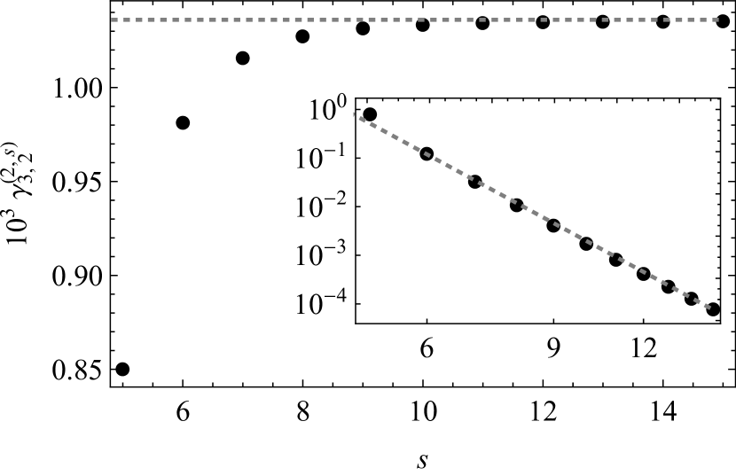
(d) $\gamma^{(2,\,s)}_{3,2}$ v. $s$

Figure 3.1: Graphical representations of the behaviour of the coefficients $\gamma^{(2,\,s)}_{m,n}$ (such that $m+n\leq 5$) as $s$ increases. The dotted straight lines indicate the results of the $s\to\infty$ extrapolations reported in table 1. The insets show on a log-log scale the decay of the increments $\gamma^{(2,\,s+1)}_{m,n}-\gamma^{(2,\,s)}_{m,n}$ as $s$ increases.

In table 1, we list, in the second column, the values of the upper bounds on the dynamic contribution to the heat conductivity $\kappa_{\textsc{d}}^{(2,\,s)}$ when restricting its computation to bivariate polynomials of degrees $s=3,\dots,\,15$. The remaining columns show the values of some of the non-trivial coefficients $\gamma^{(2,\,s)}_{m,n}$ for which the infimum is reached (the list of coefficients is limited to indices $m$ and $n$ such that $m+n\leq 6$). The values of the upper bounds on the dynamic contribution to the heat conductivity thus coincide with the values inferred from the transposition of equation (3.35) to coefficients of finite order $r=2$ and corresponding degree $s$.

The last line of table 1 lists the results of the infinite-degree extrapolations of $\kappa_{\textsc{d}}^{(2,\,s)}$ and $\gamma^{(2,\,s)}_{m,n}$ with error estimates on their last digits. To obtain those estimates, we first consider the coefficients $\gamma^{(2,\,s)}_{m,n}$ and notice their rapid convergence to asymptotic values as $s$ increases. To evaluate this convergence, we plot in figure 3.1 the graphs of the first four coefficients as functions of the degree $s$ (similar results are obtained for the other coefficients). The insets of these figures exhibit the decay of the increments $\gamma^{(2,\,s+1)}_{m,n}-\gamma^{(2,\,s)}_{m,n}$ as $s$ increases, which appear to follow simple power laws of the form $b\,s^{-c}$, and are readily fitted by linear regressions (we remove the values $s=m+n$ from the fitted sequences). The results give the respective exponent values

$$c=\begin{cases}7.07\pm 0.03\quad\mbox{(figure~{}\ref{fig:gammar2_m2n1})},\\ 7.47\pm 0.04\quad\mbox{(figure~{}\ref{fig:gammar2_m3n1})},\\ 7.85\pm 0.06\quad\mbox{(figure~{}\ref{fig:gammar2_m4n1})},\\ 8.03\pm 0.06\quad\mbox{(figure~{}\ref{fig:gammar2_m3n2})}.\end{cases}$$

The corresponding coefficients are respectively found to be $\log b=9.07\pm 0.06$, $11.0\pm 0.1$, $12.6\pm 0.1$ and $12.3\pm 0.1$. For each pair of parameters $b$ and $c$ thus obtained, we estimate the $s\to\infty$ extrapolation of $\gamma^{(2,\,s)}_{m,n}$ by adding to the last computed value, $\gamma^{(2,15)}_{m,n}$, the sum of the modeled increments,

$$\gamma^{(2,\infty)}_{m,n}\approx\gamma^{(2,15)}_{m,n}+b\sum_{s=0}^{\infty}(s+16)^{-c}\,.$$ (3.62)

The results are:

$$\gamma^{(2,\infty)}_{2,1} =6.000\,21\,, \quad\gamma^{(2,\infty)}_{3,1} =3.630\,26\,, \quad\gamma^{(2,\infty)}_{4,1} =1.961\,33\,,$$ (3.63)

$$\gamma^{(2,\infty)}_{3,2} =1.036\,07\,, \quad\gamma^{(2,\infty)}_{5,1} =1.053\,72\,, \quad\gamma^{(2,\infty)}_{4,2} =0.947\,04\,.$$ (3.64)

An alternative way of obtaining $s\to\infty$ extrapolations, which avoids resorting to the increments is to model the coefficients according to the power law $\gamma^{(r,\,s)}_{m,n}\approx a-\rme^{\log b}\,s^{-c}$. The corresponding coefficients (treating $\log b$ as such) can be evaluated through nonlinear regressions of the computed values. This procedure yields the approximations:

$$\gamma^{(2,s)}_{2,1} \approx 6.000\,30-274.409\,s^{-5.446\,98}\,, \quad\gamma^{(2,s)}_{3,1} \approx 3.630\,26-2\,168.14\,s^{-5.984\,24}\,,$$ (3.65)

$$\gamma^{(2,s)}_{4,1} \approx 1.961\,26-11\,010.0\,s^{-6.436\,06}\,, \quad\gamma^{(2,s)}_{3,2} \approx 1.036\,04-7\,585.76\,s^{-6.614\,03}\,,$$ (3.66)

$$\gamma^{(2,s)}_{5,1} \approx 1.053\,62-43\,746.1\,s^{-6.820\,7}\,, \quad\gamma^{(2,s)}_{4,2} \approx 0.946\,96-60\,580.1\,s^{-7.079\,66}\,.$$ (3.67)

The constant terms are the values reported in table 1. Although both linear and nonlinear regressions yield error estimates of the coefficients, we note that such error estimates tend to underestimate the error; systematic errors due to the chosen model must also be assessed. We thus prefer using error estimates obtained by comparing the asymptotic values given by the two different methods (3.63) and (3.65). The differences between the two are the numbers in brackets reported in table 1.

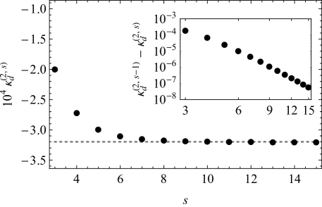
Figure 3.2: Graphical representations of the upper bounds $\kappa_{\textsc{d}}^{(2,\,s)}$ on the dynamical contribution to the heat conductivity restricted to bivariate polynomials of degree $s$ for $s=3,\dots,\,15$. The dotted straight line indicates the result of the $s\to\infty$ extrapolation reported in table 1. The inset shows on a log-log scale the decay of the decrements $\kappa_{\textsc{d}}^{(2,\,s-1)}-\kappa_{\textsc{d}}^{(2,\,s)}$ as $s$ increases.

Turning to $\kappa_{\textsc{d}}^{(2,\,s)}$, figure 3.2, we do not expect a simple power-law form will faithfully model this quantity. Indeed, the exponent values reported on the right-hand side of equation (3.65) differ significantly from each other so that $\kappa_{\textsc{d}}^{(2,\,s)}$ should rather be thought of as a sum of power laws with possibly many different exponents. Neither can we rely on our limited estimates of the coefficients $\gamma^{(2,\,\infty)}_{m,\,n}$ to compute $\kappa_{\textsc{d}}^{(2,\infty)}$: we have access to only a few of them and they do not appear to decay fast enough with $m+n$ so they could be ignored. We must somehow account for all these missing coefficients if our result is to be reliable.

It is nevertheless possible to design a transparent fitting procedure which provides results whose accuracy can be easily tested. To this end, we propose to think of $\kappa_{\textsc{d}}^{(2,\,s)}$ as approaching its asymptotic value by decrements which asymptotically fall on a power law of the type used above, $b\,s^{-c}$, and extract the asymptotic value $\kappa_{\textsc{d}}^{(2,\,\infty)}$ after estimating the parameters $b$ and $c$ as functions of $s$.

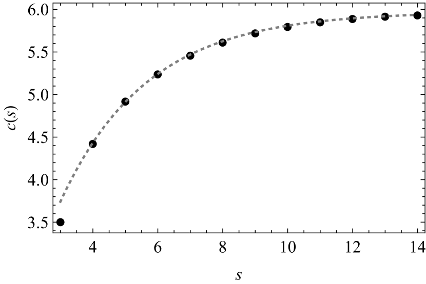
(a) $c(s)$, equation (3.68)

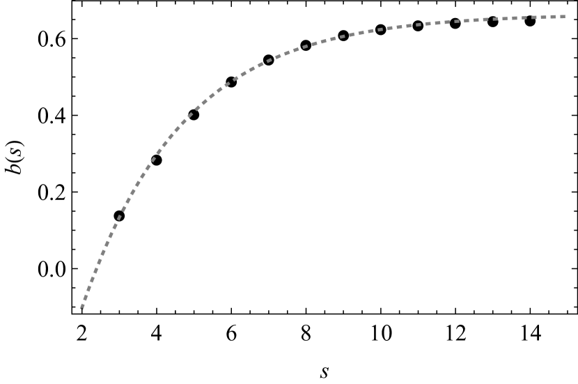
(b) $b(s)$, equation (3.70)

Figure 3.3: Exponential convergence of the fitting parameters $c(s)$, equation (3.68), and $b(s$), equation (3.70). The dotted curves show the respective fitting results (3.69) and (3.71).

The asymptotic exponent value is extracted from the computed data points by considering the decrements $\kappa_{\textsc{d}}^{(2,\,s-1)}-\kappa_{\textsc{d}}^{(2,\,s)}$, as plotted in the inset of figure 3.2, and computing

$$c(s)=\log\frac{\kappa_{\textsc{d}}^{(2,\,s)}-\kappa_{\textsc{d}}^{(2,\,s+1)}}{\kappa_{\textsc{d}}^{(2,\,s-1)}-\kappa_{\textsc{d}}^{(2,\,s)}}\Big{/}\log\frac{s}{s+1}\,.$$ (3.68)

The result is a sequence of $s$-dependent values $c(s)$ plotted in figure 3(a), which can be seen to converge exponentially fast to its asymptotic value,

$$c(s)\approx 5.974\pm 0.005-(6.8\pm 0.1)\rme^{-(0.372\pm 0.004)s}\,.$$ (3.69)

Coefficients $b(s)$ are then obtained by solving

$$b(s)=(\kappa_{\textsc{d}}^{(2,\,s-1)}-\kappa_{\textsc{d}}^{(2,\,s)})s^{c(\infty)}\,.$$ (3.70)

The result is another sequence of $s$-dependent values $b(s)$ plotted in figure 3(b), which also displays exponential convergence to its asymptotic value,

$$b(s)\approx 0.664\pm 0.004-(1.60\pm 0.05)\rme^{-(0.37\pm 0.01)s}\,.$$ (3.71)

With these quantities, we finally obtain the sought after estimated value of the dynamic contribution to the heat conductivity due to bivariate functions:

$$\kappa_{\textsc{d}}^{(2,\,\infty)}\approx\kappa_{\textsc{d}}^{(2,\,15)}-\sum_{s=16}^{\infty}b(s)s^{-c(s)}=-3.197\,13\pm 5\times 10^{-5}\,.$$ (3.72)

This is the value reported at the bottom of the second column in table 1 and the height of the horizontal dotted line shown in figure 3.2. The error estimate is inferred from the data, by comparing $\kappa_{\textsc{d}}^{(2,\,15)}$ and $\kappa_{\textsc{d}}^{(2,\,14)}-b(15)s^{-c(15)}$. The accuracy of our result is a reflection of the largest computed degree, $s=15$, and the smallness of the gap $\kappa_{\textsc{d}}^{(2,\,15)}-\kappa_{\textsc{d}}^{(2,\,\infty)}$.

Although lower than the best reported upper bound, $\kappa_{\textsc{d}}^{(2,\,15)}$, the estimate (3.72) is restricted to bivariate functions and is therefore not optimal. We can safely assume $\kappa_{\textsc{d}}<\kappa_{\textsc{d}}^{(2,\infty)}$, which will be confirmed below, and have to increase the number of variables in the trial functions to infer a confidence interval for $\kappa_{\textsc{d}}=\lim_{r,\,s\to\infty}\kappa_{\textsc{d}}^{(r,\,s)}$.

3.4 Extension to multivariate trial functions ($r>2$)

$r$	$s$	$-10^{4}\kappa_{\textsc{d}}^{(r,\,s)}$	$r$	$s$	$-10^{4}\kappa_{\textsc{d}}^{(r,\,s)}$	$r$	$s$	$-10^{4}\kappa_{\textsc{d}}^{(r,\,s)}$	$r$	$s$	$-10^{4}\kappa_{\textsc{d}}^{(r,\,s)}$
$3$	$3$	$2.247\,93$	$4$	$3$	$2.299\,71$	$5$	$3$	$2.313\,40$	$6$	$3$	$2.317\,84$
	$4$	$3.066\,36$		$4$	$3.136\,22$		$4$	$3.154\,58$		$4$	$3.160\,52$
	$5$	$3.370\,87$		$5$	$3.447\,44$		$5$	$3.467\,51$		$5$	$3.473\,99$
	$6$	$3.494\,82$		$6$	$3.574\,13$		$6$	$3.594\,90$		$6$	$3.601\,61$
	$7$	$3.549\,96$		$7$	$3.630\,50$		$7$	$3.651\,59$		$7$	$3.658\,40$
	$8$	$3.576\,50$		$8$	$3.657\,64$		$8$	$3.678\,88$		$8$	$3.685\,73$
	$9$	$3.590\,17$		$9$	$3.671\,61$		$9$	$3.692\,94$		$9$	$3.699\,81$
	$10$	$3.597\,63$		$10$	$3.679\,24$		$10$	$3.700\,61$		$10$	$3.707\,50$
	$11$	$3.601\,92$		$11$	$3.683\,62$		$11$	$3.705\,02$		$11$	$3.711\,91$
	$12$	$3.604\,49$		$12$	$3.686\,25$		$12$	$3.707\,65$		$12$	$3.714\,55$
	$13$	$3.606\,09$		$13$	$3.687\,88$		$13$	$3.709\,30$		$13$	$3.716\,20$
	$14$	$3.607\,12$		$14$	$3.688\,93$		$14$	$3.710\,35$
	$15$	$3.607\,80$		$15$	$3.689\,63$
$3$	$\infty$	$3.609\,61(6)$	$4$	$\infty$	$3.691\,48(6)$	$5$	$\infty$	$3.713\,0(1)$	$6$	$\infty$	$3.720\,1(3)$
$7$	$3$	$2.319\,52$	$8$	$3$	$2.320\,24$	$9$	$3$	$2.320\,58$	$10$	$3$	$2.320\,75$
	$4$	$3.162\,77$		$4$	$3.163\,73$		$4$	$3.164\,18$		$4$	$3.164\,41$
	$5$	$3.476\,44$		$5$	$3.477\,49$		$5$	$3.477\,98$		$5$	$3.478\,22$
	$6$	$3.604\,14$		$6$	$3.605\,22$		$6$	$3.605\,72$		$6$	$3.605\,98$
	$7$	$3.660\,96$		$7$	$3.662\,06$		$7$	$3.662\,57$		$7$	$3.662\,82$
	$8$	$3.688\,31$		$8$	$3.689\,41$		$8$	$3.689\,93$		$8$	$3.690\,18$
	$9$	$3.702\,40$		$9$	$3.703\,50$		$9$	$3.704\,02$
	$10$	$3.710\,09$		$10$	$3.711\,20$
	$11$	$3.714\,51$
$7$	$\infty$	$3.724(2)$	$8$	$\infty$	$3.727(4)$	$9$	$\infty$	$3.73(1)$	$10$	$\infty$	$3.74(3)$

Table 2: Dynamic contributions to the heat conductivity obtained from the variational formula using the trial functions (3.33) with $r$ variables and maximal degree $\sum_{i=1}^{r}n_{i}\leq s$.

To improve the upper bound (3.72) on the dynamical contribution to the heat conductivity (3.28), we must go beyond bivariate trial functions and transpose the calculations presented in section 3.3 to multivariate functions of order $r>2$. For the sake of compressing notations, given the integers $i\leq j$, we let $\underline{c}_{i:j}$ denote the sequence of indices $c_{i},\dots,c_{j}$ and $\overline{c}$ their sum, $c_{i}+\dots+c_{j}$ (we omit the indices). For functions of arbitrary number of variables $r$, the variational formula (3.42) thus becomes

$$\kappa_{\textsc{d}}^{(r,\,s)}=\mathrm{inf}_{\{\gamma^{(r,\,s)}_{\underline{c}_{1:r}}\}}\Bigg{[}\sqrt{\frac{3}{2}}\sum_{\begin{subarray}{c}m,n=1\\ m+n\leq s\end{subarray}}^{s}\gamma^{(r,\,s)}_{m,n}\,A_{m,n,1,0}+\sum_{\begin{subarray}{c}\underline{c}_{1:r-1}=0\\ \overline{c}\leq s\end{subarray}}^{s}\sum_{m,p=0}^{s-\overline{c}}\gamma^{(r,\,s)}_{\underline{c}_{1:r-1},m}\,\gamma^{(r,\,s)}_{\underline{c}_{1:r-1},p}A_{m,0,p,0}\cr+2\sum_{k=2}^{r}\sum_{\begin{subarray}{c}\underline{c}_{1:k-2}=0\\ \overline{c}\leq s\end{subarray}}^{s}\sum_{\begin{subarray}{c}n,p,q=0\\ p+q\leq s-\overline{c}\end{subarray}}^{s-\overline{c}}\frac{\gamma^{(r,\,s)}_{n,\underline{c}_{1:k-2}}\,\gamma^{(r,\,s)}_{p,q,\underline{c}_{1:k-2}}}{(r-k+1)(r-k+2)}A_{0,n,p,q}+\frac{1}{2}\sum_{k=2}^{r}\sum_{l=2}^{k}(2-\delta_{k,l})\cr\times\sum_{\begin{subarray}{c}\underline{c}_{1:r-k+l-2}=0\\ \overline{c}\leq s\end{subarray}}^{s}\sum_{\begin{subarray}{c}m,n,p,q=0\\ m+n\,\&\,p+q\leq s-\overline{c}\end{subarray}}^{s-\overline{c}}\frac{\gamma^{(r,\,s)}_{\underline{c}_{1:r-k},m,n,\underline{c}_{r-k+1:r-k+l-2}}\gamma^{(r,\,s)}_{\underline{c}_{1:r-k},p,q,\underline{c}_{r-k+1:r-k+l-2}}}{(k-l+1)^{2}}\,A_{m,n,p,q}\Bigg{]}\,.$$ (3.73)

In this expression, we have concatenated index sequences ending or beginning by sets $\underline{0}_{l}$ composed of $l$ successive $0$ according to

$$\gamma^{(r,\,s)}_{\underline{c}_{k},\underline{0}_{l}}=\gamma^{(r,\,s)}_{\underline{0}_{l},\underline{c}_{k}}=\frac{r-k-l+1}{r-k+1}\gamma^{(r,\,s)}_{\underline{c}_{k}}\,,$$ (3.74)

see (3.38), and assumed antisymmetry with respect to reversing the order of indices,

$$\gamma^{(r,\,s)}_{c_{1},\dots,c_{r}}=-\gamma^{(r,\,s)}_{c_{r},\dots,c_{1}}\,,$$ (3.75)

which also implies that coefficients with a single non-zero index must vanish, $\gamma^{(r,\,s)}_{c}\equiv 0$. As summations over the indices are performed in equation (3.73), further simplifications involving equations (3.74) and (3.75) arise.

Approximations $\kappa_{\textsc{d}}^{(r,\,s)}$ obtained by restricting the computation of the infimum in the variational formula (3.73) to multivariate polynomials of order $r$ and degree $s$ are reported in table 2.

Each one of the values listed in table 2 thus provides an analytically obtained upper bound on the actual dynamic contribution to the heat conductivity; more precisely, each such upper bound is a rational number which we report in decimal approximation to six significant digits. We may therefore conclude:

$$\kappa_{\textsc{d}}<-0.000\,371\,620\,,$$ (3.76)

which is obtained for $r=6$ and $s=13$. For this pair of parameters, the number of coefficients involved in the search of the infimum is close to $11\,000$. It is about the same number for $r=7$ and $s=11$. Such large numbers of coefficients set a bound for every $r$ on the degree $s$ for which values $\kappa_{\textsc{d}}^{(r,\,s)}$ are within reach of our computation and thus leaves out empty cells in our table.

The convergence to an asymptotic value $\kappa_{\textsc{d}}^{(r,\,\infty)}$ is observed in every column of table 2 as $s$ increases. We can therefore repeat the analysis presented in section 3.3 for $r=2$ and extend it to every value of $r=3,\dots,\,10$. The accuracy of our scheme to extrapolate to $s\to\infty$ for a given order $r$ will be tested by the reduced largest degrees for which values of $\kappa_{\textsc{d}}^{(r,\,s)}$ were computed in the last columns of the table.

Considering figure 4(a), we notice in the inset the remarkable fact that the decrements $\kappa_{\textsc{d}}^{(r,\,s-1)}-\kappa_{\textsc{d}}^{(r,\,s)}$, $3\leq r\leq 10$, appear to fall along the same curve as that observed in the inset of figure 3.2. The implication is that the exponent $c(s)$, defined in analogy to equation (3.68), must be the same function of $s$ for every $r$. By accumulating all data points, we find an improved fitting curve (3.69),

$$c(s)\approx 5.989\pm 0.003-(6.86\pm 0.06)\rme^{-(0.371\pm 0.002)s}\,.$$ (3.77)

The coefficients $b_{r}(s)$ are obtained in analogy to equation (3.70),

$$b_{2}(s) \approx 0.692\pm 0.004-(1.62\pm 0.05)\rme^{-(0.36\pm 0.01)s}\,,$$ (3.78)

$$b_{3}(s) \approx 0.774\pm 0.005-(1.84\pm 0.07)\rme^{-(0.36\pm 0.01)s}\,,$$ (3.79)

$$b_{4}(s) \approx 0.791\pm 0.006-(1.88\pm 0.07)\rme^{-(0.36\pm 0.01)s}\,,$$ (3.80)

$$b_{5}(s) \approx 0.800\pm 0.007-(1.87\pm 0.07)\rme^{-(0.36\pm 0.01)s}\,,$$ (3.81)

$$b_{6}(s) \approx 0.808\pm 0.009-(1.84\pm 0.07)\rme^{-(0.35\pm 0.01)s}\,,$$ (3.82)

$$b_{7}(s) \approx 0.82\pm 0.01-(1.81\pm 0.07)\rme^{-(0.34\pm 0.01)s}\,,$$ (3.83)

$$b_{8}(s) \approx 0.83\pm 0.02-(1.76\pm 0.06)\rme^{-(0.33\pm 0.02)s}\,,$$ (3.84)

$$b_{9}(s) \approx 0.85\pm 0.02-(1.74\pm 0.06)\rme^{-(0.31\pm 0.02)s}\,,$$ (3.85)

$$b_{10}(s) \approx 0.89\pm 0.03-(1.70\pm 0.05)\rme^{-(0.29\pm 0.02)s}\,.$$ (3.86)

They display the same kind of exponential convergence to their asymptotic values as observed in figure 3(b). For the sake of comparison, we included here $r=2$, which can be set side-by-side with equation (3.71).

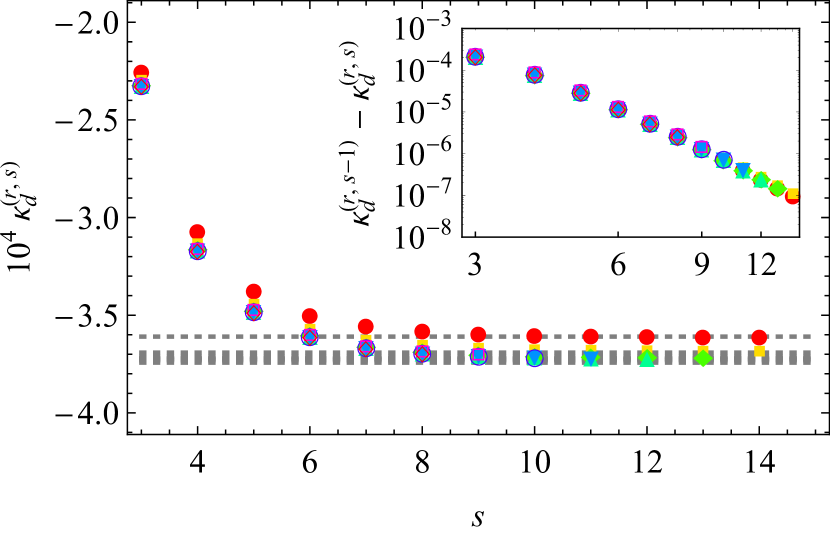
(a) $\kappa_{\textsc{d}}^{(r,\,s)}$ v. $s$  ($3\leq r\leq 10$)

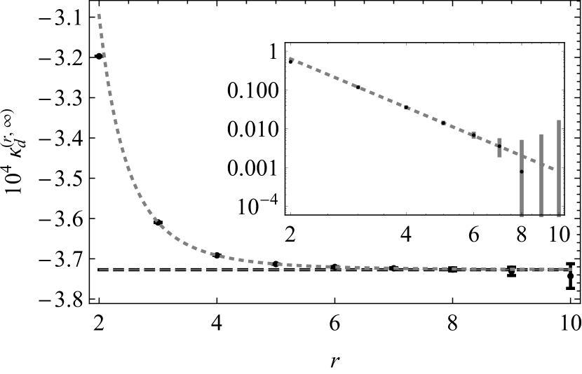
(b) $\kappa_{\textsc{d}}^{(r,\infty)}$ v. $r$

Figure 3.4: (a) Graphical representation of the upper bounds $\kappa_{\textsc{d}}^{(r,\,s)}$ on the dynamical contribution to the heat conductivity reported in table 2 for $r=3,\dots,\,10$. (b) Estimate of $\kappa_{\textsc{d}}=\lim_{r\to\infty}\kappa_{\textsc{d}}^{(r,\infty)}$ by the nonlinear power-law fit (3.87). In both panels, the dotted straight lines indicate the results of the extrapolations $s\to\infty$ (a) and $r\to\infty$ (b).

With these quantities, we proceed in analogy to equation (3.72) to obtain estimates of the dynamic contributions to the heat conductivity due to $r$-variate functions, $\kappa_{\textsc{d}}^{(r,\,\infty)}$. The values are reported in table 2. They correspond to the heights of the horizontal dotted lines shown in figure 4(a) and are the data points of figure 4(b) on which the $r\to\infty$ extrapolation is based. The error estimates are inferred from the data, by comparing $\kappa_{\textsc{d}}^{(r,\,s_{\mathrm{max}})}$ and $\kappa_{\textsc{d}}^{(r,\,s_{\mathrm{max}-1})}-b_{r}(s_{\mathrm{max}})s^{-c(s_{\mathrm{max}})}$, where, for each $r$, $s_{\mathrm{max}}$ is the largest degree $s$ for which $\kappa_{\textsc{d}}^{(r,\,s)}$ was computed. Here we note that the differences between the parameter $b_{2}(s)$ in equation (3.78) and $b(s)$ in equation (3.71) would have the effect of changing the last digit reported in $\kappa_{\textsc{d}}^{(2,\,\infty)}$ by one unit less, which is well within the corresponding error estimate (which remains unchanged).

Next we turn to the $r\to\infty$ extrapolation of $\kappa_{\textsc{d}}^{(r,\,\infty)}$, which is the dynamic contribution to the heat conductivity (2.29). The values of the estimated contributions from $r$-variate functions are reported in figure 4(b). As seen from the inset the decrements $\kappa_{\textsc{d}}^{(r-1,\,\infty)}-\kappa_{\textsc{d}}^{(r,\,\infty)}$ appear to follow a power law whose exponent is between $-4$ and $-5$, sufficiently different from an integer value that we have to resort to a nonlinear regression of the model. The result of this fit, which excludes $r=2$, yields

$$\kappa_{\textsc{d}}^{(r,\,\infty)}\approx-0.000\,372\,72\pm 6\times 10^{-8}+(0.001\,12\pm 5\times 10^{-5})\,r^{-4.14\pm 0.04}\,.$$ (3.87)

It is shown as the dotted curve in figure 4(b) (as well as the inset for the algebraic decay); the dashed horizontal line is the asymptotic value, $\kappa_{\textsc{d}}^{(\infty,\,\infty)}$. The $95\%$ confidence interval of the first parameter gives our best estimate of the dynamical contribution to equation (3.28) ,

$$-0.000\,372\,87<\kappa_{\textsc{d}}<-0.000\,372\,58\,.$$ (3.88)

The inferred estimated value of the dynamic contribution $\kappa_{\textsc{d}}=-0.000\,372\,72(6)$, with seven significant decimals, is consistent with the upper bound (3.76).

Our analysis of the coefficients $\gamma^{(r,\,s)}_{m,\,n}$, equation (3.65) carries over to $r>2$. The values obtained by the $s\to\infty$ extrapolation are shown graphically in figure 3.5 for all pairs $\{m,\,n\}$ such that $m+n\leq 7$. To estimate the $r\to\infty$ extrapolations, we fit these values by nonlinear regressions with power laws $\gamma^{(r,\,\infty)}_{m,n}\approx a+b\,r^{-c}$. The results (excluding $r=2$) are as follows:

$$\gamma^{(\infty,\,\infty)}_{2,\,1} =0.007\,040\,3\pm 4\times 10^{-7}\,, \qquad\gamma^{(\infty,\,\infty)}_{3,\,1} =0.004\,184\,3\pm 1\times 10^{-7}\,,$$ (3.89)

$$\gamma^{(\infty,\,\infty)}_{4,\,1} =0.002\,241\,6\pm 1\times 10^{-7}\,, \qquad\gamma^{(\infty,\,\infty)}_{3,\,2} =0.001\,164\,46\pm 3\times 10^{-8}\,,$$ (3.90)

$$\gamma^{(\infty,\,\infty)}_{5,\,1} =0.001\,202\,5\pm 2\times 10^{-7}\,, \qquad\gamma^{(\infty,\,\infty)}_{4,\,2} =0.001\,054\,7\pm 2\times 10^{-7}\,,$$ (3.91)

$$\gamma^{(\infty,\,\infty)}_{6,\,1} =0.000\,660\,7\pm 4\times 10^{-7}\,, \qquad\gamma^{(\infty,\,\infty)}_{5,\,2} =0.000\,756\,3\pm 5\times 10^{-7}\,,$$ (3.92)

$$\gamma^{(\infty,\,\infty)}_{4,\,3} =0.000\,344\,6\pm 9\times 10^{-7}\,.$$ (3.93)

The error estimates reported here are those returned by the nonlinear regression. The respective contributions of these coefficients to the thermal conductivity (3.35) are, up to a minus sign, $0.000\,262\,4$, $0.000\,072\,2$, $0.000\,017\,1$, $0.000\,005\,6$, $0.000\,004\,1$, $0.000\,004\,2$, $0.000\,001\,0$, $0.000\,001\,9$, and $0.000\,000\,5$, whose total, $0.000\,369\,0$, accounts for about $99\%$ of the conductivity (3.88).

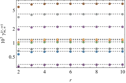
Figure 3.5: Graphical representation on a semi-log scale of the extrapolated coefficients $\gamma^{(r,\,\infty)}_{m,\,n}$ as functions of $r$. The straight lines show the $r\to\infty$ estimates, equation (3.89).

It would of course be desirable to improve our computation and go beyond the limited order and degree values reported here. This would allow us to refine our extrapolation and check the validity of the model and the precision of the result. While we have to leave such considerations to future work, we can turn to simulations of the nonequilibrium steady state to obtain an independent estimate on the dynamic contribution to the heat conductivity.

4 Kinetic Monte Carlo simulations

The nonequilibrium steady state of the stochastic model can be simulated following along the lines of Gillespie’s kinetic Monte Carlo algorithm [24]. This yields a numerical determination of the heat conductivity through Fourier’s law (2.7), which can be compared with the theoretical results described in section 3.4.

The method is an improved version of that described in references [7, 8]. We consider a one-dimensional chain of $N$ cells, with both ends in contact with thermal reservoirs at different temperatures, which we take to be $T_{-}=\tfrac{1}{2}$ at cell $-(N+1)/2$ and $T_{+}=\tfrac{3}{2}$ at cell $(N+1)/2$. Their energies are thus distributed according to Gamma distributions of shape parameter $\tfrac{3}{2}$ and scale parameters $T_{\pm}$. Rather than draw a random energy from these distributions at large enough (constant) rate to simulate the constant temperature of the reservoirs, it is more precise (as well as it saves computer time) to consider the integrated form of the kernel (3.23) with respect to these distributions, which yields a thermalized kernel for the interaction of cells $\pm(N+1)/2$ with the thermostats at temperatures $T_{\pm}$,

$$w_{T}(e|e+h)=\sqrt{\frac{\pi}{8\,e}}\times\begin{cases}0,&h<-e,\\ \rme^{h/T}\mathrm{erf}\left(\sqrt{\frac{e+h}{T}}\right)\,,&-e\leq h<0,\\ \mathrm{erf}\left(\sqrt{\frac{e}{T}}\right)\,,&h\geq 0,\end{cases}$$ (4.1)

where $\mathrm{erf}$ denotes the error function. A moderate price to pay for this implementation is the numerical determination of the amount of energy exchanged with the thermostats by the rejection method [25, section 7.3.6].

At each Monte Carlo step, the time until the next energy exchange event and the pair involved (including thermostats) is determined from a collection of clocks associated with each pair of cells. For each one of them, the frequency $\nu(e_{n},e_{n+1})$ specifies the exponential rate of the random distribution from which the time to the next interaction is generated. For cells in contact with thermal baths, this rate is

$$\nu_{T}(e)=\sqrt{\frac{T}{8}}\left[\rme^{-e/T}+\sqrt{\frac{\pi\,T}{e}}\left(\frac{1}{2}+\frac{e}{T}\right)\mathrm{erf}\left(\sqrt{\frac{e}{T}}\right)\right]\,,$$ (4.2)

where $T=T_{\pm}$. Whenever a clock rings, a uniformly-distributed random number is generated, which, by inversion of the partially integrated kernel, yields the amount of energy exchanged between the two interacting cells. Their clocks are then renewed, along with those of the relevant neighbouring pairs. At each step, the energies

$$\{e_{-(N-1)/2},\,e_{-(N-3)/2},\dots,\,e_{(N-3)/2},\,e_{(N-1)/2}\}$$ (4.3)

in the $N$ cells are so updated while keeping the temperature of the thermostats constant.

To measure the average heat flux, we compute the average of the current (3.26), estimating $\left\langle j(e_{n},e_{n+1})\right\rangle_{\textsc{neq}}$ between every pair of cells by a time integral. These $N+1$ pairs include the two thermostats, for which we obtain the average current exchanged with the boundary cell by integrating the current (3.26) with respect to the Gamma distribution associated with the reservoir,

$$j_{T}(e)=\frac{T^{5/2}}{4\sqrt{2}\,e}\left[\frac{e}{T}\left(\frac{3}{2}-\frac{e}{T}\right)\rme^{-e/T}+\sqrt{\pi}\sqrt{\frac{e}{T}}\left(\frac{5}{4}+\frac{e}{T}-\frac{e^{2}}{T^{2}}\right)\mathrm{erf}\left(\sqrt{\frac{e}{T}}\right)\right]\,.$$ (4.4)

The average total current, which we denote $J_{\textsc{h}}$, is defined as the sum of all these contributions,

$$J_{\textsc{h}}(N)=\sum_{n=-(N+1)/2}^{(N-1)/2}\left\langle j(e_{n},e_{n+1})\right\rangle_{\textsc{neq}}\,.$$ (4.5)

Measurements of this quantity are graphically illustrated in figure 1(a) for system sizes ranging from $N=1,\dots,\,256$.

(a) Total current

(b) Temperature gradient

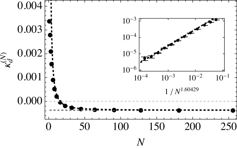
(c) Finite-size dynamic contribution

Figure 4.1: (a) Total current $J_{\textsc{h}}$ v. $N$ (4.5) for system sizes of up to $N=256$ cells resulting from the nonequilibrium boundary conditions at temperatures $T_{-}=\tfrac{1}{2}$ and $T_{+}=\tfrac{3}{2}$. (b) Sum of the local temperature gradient, $T_{n+1}-T_{n}$, weighted by the square root of the mean temperature $T_{n,\,n+1}$, as it appears in the denominator of the right-hand side of equation (4.6). (c) Finite-size dynamic contribution to the heat conductivity, $\kappa_{\textsc{d}}^{(N)}$, and the result of its extrapolation to infinite size (4.7). The inset shows the power-law convergence towards the estimated asymptotic value $-0.000\,371$.

The heat conductivity is obtained from the above quantity through the local expression of Fourier’s law, $\kappa^{(N)}(T_{n,n+1})\nabla T_{n,n+1}=-\left\langle j(e_{n},e_{n+1})\right\rangle_{\textsc{neq}}$, where $\nabla T_{n,n+1}\equiv T_{n+1}-T_{n}$ is the difference of local temperatures between neighbouring cells, which are defined according to equation (2.4), and $T_{n,n+1}$ is the arithmetic average between the two local temperatures. Summing over all cells and extracting the square-root temperature dependence of the heat conductivity, we may thus write

$$\frac{\kappa^{(N)}(T)}{\sqrt{T}}=-\frac{J_{\textsc{h}}(N)}{\sum_{n}\sqrt{T_{n,n+1}}\nabla T_{n,n+1}}\,.$$ (4.6)

The measured numerator and denominator of the right-hand side of this equation are separately plotted in figure 4.1. By taking their ratio and subtracting the static contribution, we obtain the dynamic contribution to the heat conductivity as a function of the system size; see figure 1(c). An extrapolation to infinite-system size by a power-law nonlinear fit (excluding $N\leq 45$) yields the result

$$\kappa_{\textsc{d}}^{(N)}\approx-0.000\,371\pm 2\times 10^{-6}+(0.03\pm 0.01)N^{-1.6\pm 0.1}\,.$$ (4.7)

The power-law convergence of the data is displayed in the inset of figure 1(c). The $95\%$ confidence interval of the first parameter gives the $N\to\infty$ estimate of the dynamical contribution to the heat conductivity,

$$-0.000\,377\leq\kappa_{\textsc{d}}\leq-0.000\,365\,.$$ (4.8)

The center of this interval is slighted shifted with respect to the values found in section 3.4 by application of the variational formula. Its width is however substantially larger and contains the confidence interval (3.88). Moreover the upper bound on the right-hand side of equation (4.8) is larger than the explicit upper bound (3.76), which is a reminder that the interval inferred from Monte Carlo simulations is not as precise as the found by application of the variational formula.

We close this section with a brief aside. We argued in section 2.2 that the contribution to the probability density of the steady state given by equation (2.32) should be understood as the part of the nonequilibrium steady state contributing to the current. The coefficients $\gamma_{\dots,0,n_{0},n_{1},0,\dots}$ of its expansion in terms of Laguerre polynomials turn out to be antisymmetric with respect to the exchange of the two indices $n_{0}$ and $n_{1}$, so that the function which realizes the infimum in the variational formula (3.14) does not contribute to symmetric observables of two variables. This however leaves open the possibility that the two-cell marginal density distribution of the actual steady state may have a symmetric part the variational formula comes short of revealing.

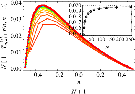
Figure 4.2: Deviations of $\nu(n,\,n+1)$, the measured collision frequency in the nonequilibrium steady state, from its local equilibrium value, $T_{n,\,n+1}^{1/2}$ multiplied by the system size, $N$. Values from $N=8$ to $N=256$ are shown in different colors. Inset: average with respect to $n$, $-(N+1)/2\leq n\leq(N-1)/2$, of this quantity as a function of $N$. The dashed line shows the power-law fit $0.019\,988-0.044\,0766\,N^{-1}$, obtained by nonlinear regression restricted to $N>45$.

The energy exchange frequency (2.27) is such a symmetric observable. In figure 4.2 we let $\nu(n,\,n+1)$ denote its ensemble average between cells $n$ and $n+1$ and analyze its deviations from the local equilibrium contribution $T_{n,\,n+1}^{1/2}$ as the size of the system varies. More precisely, we multiply the difference $1-T_{n,\,n+1}^{-1/2}\,\nu(n,\,n+1)$ by $N$ and estimate the behaviour of this quantity when $N\gg 1$. The inset of the figure shows how its average converges to an asymptotic value which our analysis estimates to be in the interval $[0.019\,922,\,0.020\,054]$ with a power-law convergence in $N^{-1}$. We infer from this that symmetric contributions to the two-cell marginal density distribution of the steady state must vanish to first order in the gradient expansion.

5 Conclusion

We have presented an improved calculation of the heat conductivity of the energy exchange stochastic model associated with a system of locally confined hard spheres at the conductor-insulator threshold. Sasada’s transposition of the variational formula to such a system [14, 15, 16] provides an efficient instrument to obtain successive exact upper bounds for the heat transport coefficient, whose values can be extrapolated to infer an interval of confidence of the dynamic contribution to this quantity. Comparisons of this result with values of the heat conductivity associated with a nonequilibrium steady state obtained by kinetic Monte Carlo simulations were presented, displaying excellent agreement, especially with regards to the smallness of the numbers reported.

The calculation thus contradicts the conjecture we made earlier in references [5, 6, 7, 8, 9] that the heat conductivity should be equal to the binary collision frequency. The implication would be that the dynamic contribution to the conductivity should vanish, as it does in gradient systems [16]. The present results demonstrate that this is not the case. The ratio of the heat conductivity and square root of temperature is indeed slightly smaller than the scaled collision frequency, with a deviation estimated to be $-0.000\,372\,72(6)$ from our analysis of the variational formula. Our Monte Carlo simulations corroborate this result, although with a lesser precision, consistent to within six significant decimals, $\kappa(T)-\nu(T)\simeq-0.000\,373\sqrt{T}$.

The variational formula thus provides a potent tool to compute this correction. As our results illustrate, the kinetic Monte Carlo simulations are not as precise. Going to larger system sizes seems to be necessary, but growing computer times are difficult to manage. This observation is also reflected by the values of the exponents inferred from our power-law fits, which are substantially larger (in absolute value) for the order and degree in the variational formula compared to that of the system size in the kinetic Monte Carlo simulations.

Similar results hold for the two-dimensional hard-disc system. In this case, we obtain the exact upper bound $\kappa_{\textsc{d}}<\kappa_{\textsc{d}}^{(6,14)}=-0.000\,893\,56$, which suggests that the dynamical correction to the heat conductivity is about twice as large for this case than the one investigated here. Kinetic Monte Carlo simulations using the stochastic kernel associated with two-dimensional discs are however much slower as they involve a numerical root-finding algorithm to determine the amount of energy exchanged when two cells interact. We suspect that the stochastic energy-exchange process associated with a system mixing two-dimensional balls and one-dimensional pistons in a regime of rare interactions [10] has a coefficient of heat conductivity with a dynamic contribution larger still. However, technical problems due to the mixed nature of this system have yet to be overcome before the derivation of the variational formula can be transposed to such systems.

References

References

- [1] Bunimovich L A and Sinai Y G 1981 Communications in Mathematical Physics 78 479–497 URL http://dx.doi.org/10.1007/BF02046760
- [2] Bunimovich L A, Sinai Y G and Chernov N 1991 Russian Mathematical Surveys 46 47–106 URL http://dx.doi.org/10.1070/RM1991v046n04ABEH002827
- [3] Chernov N 1994 Journal of Statistical Physics 74 11 URL http://dx.doi.org/10.1007/BF02186805
- [4] Bunimovich L A, Liverani C, Pellegrinotti A and Suhov Y M 1992 Communications in Mathematical Physics 146 357 URL http://dx.doi.org/10.1007/BF02102633
- [5] Gaspard P and Gilbert T 2008 Physical Review Letters 101 20601 URL http://dx.doi.org/10.1103/PhysRevLett.101.020601
- [6] Gaspard P and Gilbert T 2008 New Journal of Physics 10 3004 URL http://dx.doi.org/10.1088/1367-2630/10/10/103004
- [7] Gaspard P and Gilbert T 2008 Journal of Statistical Mechanics 11 021 URL http://dx.doi.org/10.1088/1742-5468/2008/11/P11021
- [8] Gaspard P and Gilbert T 2009 Journal of Statistical Mechanics 08 020 URL http://dx.doi.org/10.1088/1742-5468/2009/08/P08020
- [9] Gaspard P and Gilbert T 2012 Chaos 22 026117 URL http://dx.doi.org/10.1063/1.3697689
- [10] Bálint P, Gilbert T, Nándori P, Szász D and Tóth I P 2016 Journal of Statistical Physics 1–23 ISSN 1572-9613 URL http://dx.doi.org/10.1007/s10955-016-1598-5
- [11] Sasada M 2015 The Annals of Probability 43 1663–1711 URL http://dx.doi.org/10.1214/14-AOP916
- [12] Grigo A, Khanin K and Szász D 2012 Nonlinearity 25 2349–2376 URL http://dx.doi.org/10.1088/0951-7715/25/8/2349
- [13] Gilbert T and Lefevere R 2008 Physical Review Letters 101 200601 URL http://doi.org/10.1103/PhysRevLett.101.200601
- [14] Sasada M 2016 arXiv:1611.08866 [math-ph] URL https://arxiv.org/abs/1611.08866
- [15] Spohn H 1990 Journal of Statistical Physics 59 1227–1239 ISSN 1572-9613 URL http://dx.doi.org/10.1007/BF01334748
- [16] Spohn H 1991 Large Scale Dynamics of Interacting Particles Theoretical and Mathematical Physics (Springer Berlin Heidelberg) ISBN 9783642843730 URL http://link.springer.com/book/10.1007%2F978-3-642-84371-6
- [17] Varadhan S R S 1993 Nonlinear diffusion limit for a system with nearest neighbor interactions. II Asymptotic problems in probability theory: stochastic models and diffusions on fractals (Pitman Research Notes in Mathematics no 283) ed Elworthy K D and Ikeda N (Essex, England: Longman Scientific & Technical) pp 75–128 "Proceedings of the Taniguchi international symposium, Sanda and Kyoto, 1990."
- [18] Varadhan S R S and Yau H T 1997 The Asian Journal of Mathematics 1 623–678 URL http://intlpress.com/site/pub/files/_fulltext/journals/ajm/1997/0001/0004/AJM-1997-0001-0004-a001.pdf
- [19] Helfand E 1960 Physical Review 119 1–9 URL http://dx.doi.org/10.1103/PhysRev.119.1
- [20] Pinsky M A and Karlin S 2011 An Introduction to Stochastic Modelling fourth edition ed (Boston: Academic Press) ISBN 978-0-12-381416-6 URL http://www.sciencedirect.com/science/book/9780123814166
- [21] Basile G, Bernardin C and Olla S 2009 Communications in Mathematical Physics 287 67–98 ISSN 1432-0916 URL http://dx.doi.org/10.1007/s00220-008-0662-7
- [22] Bateman H 1953 Higher transcendental functions The Bateman Manuscript project vol 2 ed Erdélyi A (McGraw-Hill Book Company) URL http://authors.library.caltech.edu/43491/
- [23] Taylor B N and Mohr P J 1999 The NIST reference on constants, units and uncertainty (NIST) URL http://physics.nist.gov/cuu/index.html
- [24] Gillespie D T 1976 Journal of Computational Physics 22 403–434 URL http://dx.doi.org/10.1016/0021-9991(76)90041-3
- [25] Press W H, Teukolsky S A, Vetterling W T and Flannery B P 2007 Numerical Recipes in C: the art of scientific computing (Cambridge: Cambridge University Press) URL http://www.cambridge.org/9780521880688